Rethinking and Benchmarking Predict-then-Optimize Paradigm for Combinatorial Optimization Problems

Abstract.

Numerous web applications rely on solving combinatorial optimization problems, such as energy cost-aware scheduling, budget allocation on web advertising, and graph matching on social networks. However, many optimization problems involve unknown coefficients, and improper predictions of these factors may lead to inferior decisions which may cause energy wastage, inefficient resource allocation, inappropriate matching in social networks, etc. Such a research topic is referred to as “Predict-Then-Optimize (PTO)” which considers the performance of prediction and decision-making in a unified system. A noteworthy recent development is the end-to-end methods by directly optimizing the ultimate decision quality which claims to yield better results in contrast to the traditional two-stage approach. However, the evaluation benchmarks in this field are fragmented and the effectiveness of various models in different scenarios remains unclear, hindering the comprehensive assessment and fast deployment of these methods. To address these issues, we provide a comprehensive categorization of current approaches and integrate existing experimental scenarios to establish a unified benchmark, elucidating the circumstances under which end-to-end training yields improvements, as well as the contexts in which it performs ineffectively. We also introduce a new dataset for the industrial combinatorial advertising problem for inclusive finance to open-source. We hope the rethinking and benchmarking of PTO could facilitate more convenient evaluation and deployment, and inspire further improvements both in the academy and industry within this field.

1. Introduction

Many web-based applications depend on solving combinatorial optimization (CO) problems, such as energy cost-aware scheduling (Wahdany et al., 2023), vehicle routing (Lu et al., 2019), budget allocation on websites for information dissemination (Wilder et al., 2019), portfolio optimization (Markowitz and Todd, 2000), and graph matching on social networks (Kazemi et al., 2015). However, in many cases, the coefficients used to construct an optimization objective are unknown at the time of solving or deployment. Without proper predictions, decisions may lead to unfavorable consequences. For example, the utilization of clean energy sources has resulted in more frequent fluctuations in energy demand and prices. In the energy cost-aware scheduling problem, neglecting energy prices and deploying scheduling tasks during periods of elevated energy costs would significantly escalate expenses and result in higher energy consumption. Negative consequences without adequate predictions in other applications of CO include unnecessary expenditure on advertising budget, inappropriate social matching, inadequate financial services for specific population groups, and suboptimal portfolio allocation, which may impede circulation of capital in society and hinder economic growth.

Hence, it highlights the necessity for an integrated system that incorporates both prediction and decision-making for comprehensive consideration. Recently, predict-then-optimize (Elmachtoub and Grigas, 2022; Mandi et al., 2020; Cameron et al., 2022) (PTO, or decision-focused learning (Wilder et al., 2019; Mandi et al., 2022; Shah et al., 2022)) has gained increasing attention within the research community. In contrast with recent machine learning (ML)-based solvers for CO problems (e.g. solving traveling salesman problem (Qiu et al., 2022)) which focuses on improving the solving process through ML techniques, PTO is centered around obtaining a better prediction tailored for the final decision quality, where the solver itself is usually not the major concern.

Figure 1. Example of PTO in Energy-cost aware scheduling. Factories estimate future energy prices in the prediction stage and deploy job schedules in the optimization stage. Using properly predicted energy prices for scheduling may greatly reduce energy consumption during this process.

A basic solution to PTO follows a two-stage approach, as shown in Figure 2, which first predicts coefficients of the optimization task through a predictive model trained under the supervision of ground truth coefficients, and subsequently utilizes off-the-shelf solvers to obtain the solutions. Intuitively, it is expected that a higher prediction accuracy would result in better decision quality in PTO. Nonetheless, as evidenced by Figure 8, there often exists a gap between prediction objectives and ultimate optimization goals, leading to suboptimal decisions by two-stage methods. Therefore, a recent series of studies (Wilder et al., 2019; Wang et al., 2020; Mandi et al., 2022; Shah et al., 2022) has proposed to design an end-to-end training paradigm oriented towards the ultimate decision objective, which exhibited notable improvement over the traditional two-stage approach in many applications of PTO.

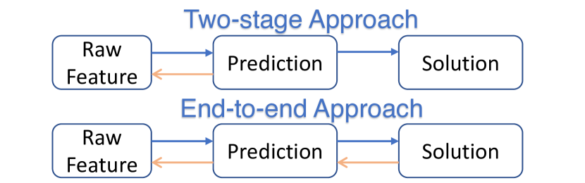
Figure 2. Paradigm of end-to-end training of prediction and optimization models. In contrast to the conventional two-stage predict-then-optimize approach, recent work has employed the design of a loss function to achieve end-to-end training oriented to the ultimate objective.

The main challenges towards the end-to-end training in PTO for combinatorial optimization problems lie in two aspects: (1) the solution’s derivatives with respect to the optimization coefficients are not available. (2) the variables in the optimization problems are discrete. Both challenges lead to the blocking of gradients. To mitigate this issue, several approaches have been proposed including designing proxy loss functions (Mandi et al., 2020), gradient approximation (Pogančić et al., 2019), etc. However, there lacks a systematic categorization of existing methods, and it is not clear which methods are effective for specific problems and scenarios. Moreover, the experimental benchmarks are relatively fragmented, and the existing proposed models have not undergone comprehensive evaluation, impeding the research community’s progression. Though some framework implementations (Agrawal et al., 2019a; Tang and Khalil, 2022) are available for some methods, they only support linear or convex problems, while overlooking other non-linear and submodular problems. Moreover, the optimization problems in PTO datasets are limited in scale and some of them use generated data for the prediction part, lacking an industrially large-scale real dataset for validating end-to-end performance.

In this work, we systematically review existing methodologies and establish a benchmark to align them. We also conduct a series of in-depth experiments to explore the capabilities of end-to-end training models including constraint satisfaction, generalization ability, adaptability to varying decision sizes, etc. We anticipate that our open-source benchmark and dataset will gain increased attention, thereby fostering advancements in both research and practical applications. Our contributions are summarized as follows:

$\bullet$   Regarding several topics including energy conservation, efficient budget allocation, and inclusive finance, we bring the end-to-end training paradigm within the Predict-Then-Optimize (PTO) formulation. We systematically review current research on PTO on combinatorial optimizations and categorize it into four distinct classes according to how the problem is solved and how the loss function is designed: discrete, continuous, statistical, and surrogate.

$\bullet$   We establish a modular framework that would be publicly available to the community, encompassing 8 problems, 11 methods, and multiple solvers to comprehensively evaluate the existing methods. We also bring a new industrial benchmark regarding the combinatorial advertising problem for inclusive finance, formulated as an integer linear program.

$\bullet$   We conduct a series of experiments to explore which scenarios the end-to-end training brings benefits, as well as the scenarios that the end-to-end training fails. Our experimental results reveal that current approaches may perform inadequately when facing more stringent constraints, larger decision variable sizes, and the need for generalization across diverse optimization parameters.

Table 1. Comparison of representative approaches for each class towards end-to-end training of PTO, where BB, ID, CPLayer is short for Blackbox, Identity, and cvxpy layer. Each approach possesses the capability to address specific optimization objectives and constraints.

Predictive

Discrete

Continuous

Statistical

Surrogate

On-the-fly

✓

✓

✓

✗

✗

$\partial\mathbf{z}/\partial\mathbf{y}$

None

Innate

Interpolation

Automatic differentiation

Designed

Statistical

Learned

Approach

Two-stage

DFL (Shah et al., 2022)

BB (Pogančić et al., 2019)

ID (Sahoo et al., 2023)

QPTL (Wilder et al., 2019)

CPLayer (Agrawal et al., 2019a)

SPO+ (Mandi et al., 2020)

NCE (Mulamba et al., 2021)

LTR (Mandi et al., 2022)

LODL (Shah et al., 2022)

Objective

Any

Any

Linear

Linear

Quadratic

Convex

Linear

Any

Any

Constraints

Any

Any

Linear

Linear

Linear

Convex

Linear

Any

Any

Additional solving

0

0

1

0

0

0

1

Multiple

Multiple

2. Problem Formulation

Consider a combinatorial optimization problem formulated as:

(1) $$\max_{\mathbf{z}\in\mathcal{Z}}\quad f(\mathbf{z},\mathbf{y},\bm{\theta})~{}s.t.~{}\operatorname{Constr}(\mathbf{z},\bm{\theta})~{},$$

where $f(\mathbf{z},\mathbf{y},\bm{\theta})$ denotes the optimization objective (abbreviated as $f(\mathbf{z},\mathbf{y})$ in the following) with discrete variable $\mathbf{z}\in\mathcal{Z}$, and $\mathbf{y}$ is the collection of unknown optimization coefficients, $\bm{\theta}$ are the optimization parameters that are known and fixed, and $\operatorname{Constr}(\mathbf{z},\bm{\theta})$ are the constraints. In this paper, we assume that the coefficients of the constraints are known. We denote one solver call for a problem instance with coefficient $\mathbf{y}$ as $\mathbf{z}(\mathbf{y})$, and $\mathbf{z}^{\star}(\mathbf{y})$ as the optimal solution. Possible solvers include commercial solvers (e.g. Gurobi (Gurobi, 2019)), open-sourced solvers (e.g. cvxpy (Diamond and Boyd, 2016)), or neural solvers (e.g. submodular (Karimi et al., 2017)), which are specific to the optimization problem. In this work, we focus on PTO for combinatorial optimization problems.

Though the coefficient $\mathbf{y}$ is unknown, in many circumstances it could be estimated from a collection of historical or pre-collected instance set $D=\{(\mathbf{x}_{i},\mathbf{y}_{i})\}$ where $\mathbf{x}$ denotes the relevant raw features. Therefore, the learning process of the prediction step of the two-stage approach could be formulated as:

(2) $$\min\mathbb{E}_{(\mathbf{x}_{i},\mathbf{y}_{i})\sim D}[\mathcal{L}_{pred}(\hat{\mathbf{y}}_{i},\mathbf{y}_{i})]~{},$$

where $\mathcal{L}_{pred}$ is a training loss specified according to the prediction output, e.g. mean squared error (MSE). Suppose the prediction model $\mathcal{M}$ serves as a mapping from the feature vector $\mathbf{x}_{i}$ to coefficients $\hat{\mathbf{y}}_{i}$, i.e. $\hat{\mathbf{y}}_{i}=\mathcal{M}(\mathbf{x}_{i})$, the overall predict-then-optimize problem formulates as:

(3) $$\underset{\mathbf{z}_{i}\in\mathcal{Z}}{\max}\quad\mathbb{E}_{(\mathbf{x}_{i},\mathbf{y}_{i})\sim D}\left[f\left(\mathbf{z}_{i}(\mathcal{M}(\mathbf{x}_{i})),\mathcal{M}(\mathbf{x}_{i}),\bm{\theta}\right)\right].$$

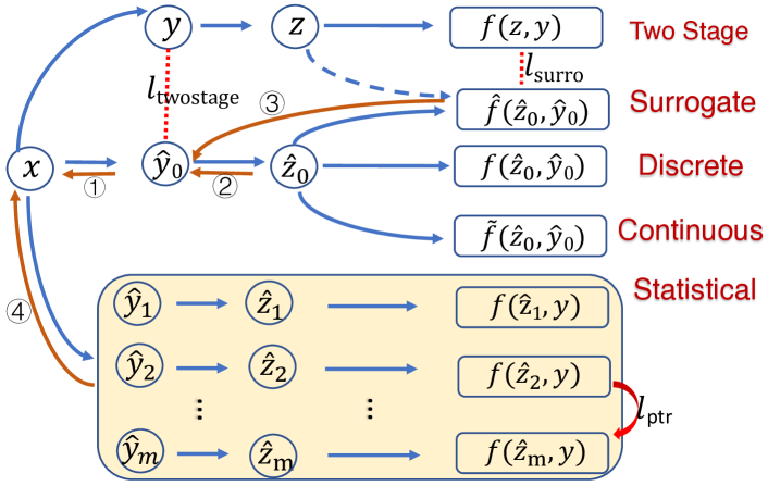
Figure 3. Gradient flow of existing methods for PTO, where $f$, $\hat{f}$ and $\tilde{f}$ denote the original objective, learned objective by surrogate model, and the continuous relaxation of the original objective, respectively. The path of back propagation of the vanilla two-stage is ①, while discrete/continuous classes use ①②, statistical class uses  ④, and surrogate class uses  ①③.

The evaluation of the PTO could be critical. In many circumstances where the coefficients of the test set are available, regret is used to evaluate decision quality. Let the decision quality (Shah et al., 2022; Ferber et al., 2023) of solution $\hat{\mathbf{z}}$ be the objective under the ground-truth coefficient $\mathbf{y}$:

(4) $$\operatorname{DQ}(\hat{\mathbf{z}})=f(\hat{\mathbf{z}},\mathbf{y},\bm{\theta}).$$

Then the regret could be obtained by the difference of the decision quality with solutions under the estimated coefficient($\mathbf{z}^{\star}(\mathbf{y}),$ and ground-truth coefficients ($\mathbf{z}^{\star}(\hat{\mathbf{y}})$):

(5) $$Regret(\hat{\mathbf{y}},\mathbf{y})=|f(\mathbf{z}^{\star}(\mathbf{y}),\mathbf{y},\bm{\theta})-f(\mathbf{z}^{\star}(\hat{\mathbf{y}}),\mathbf{y},\bm{\theta})|.$$

However, in many cases, the ground truth coefficients $y$ are not readily available or even impossible to obtain, so the evaluation of PTO becomes challenging. Online A/B testing may be one approach, however, associated with higher costs and risks. Consequently, we propose using uplift, an offline controlled variable metric common in causal inference tasks as an alternative evaluation, where the details are left in the combinatorial advertising problem.

3. Discussion on Existing Methods

As briefly introduced earlier, the major challenges toward the end-to-end learning of prediction and optimization lie in two aspects: (1) unavailable informative gradients and (2) discrete variables. These two challenges block the gradient backpropagation of the optimization task so that the prediction model cannot update with the final objective. To address these challenges, as shown in Table 1, we categorize existing works into four classes according to how the optimization is solved and how the gradient is obtained, where the gradient flow of these approaches is shown in Figure 3. We consider the Two-stage training as a baseline method, while concurrently note that the first challenge can be readily addressed if the solver itself is differentiable, such as neural solvers for top-k problems (Xie et al., 2020) or the Sinkhorn algorithm (Sinkhorn, 1964) used in neural graph matching (Wang et al., 2019).

3.1. The Discrete Class

The “discrete” class solves the optimization problem with the original discrete solver. As discussed in previous works (Pogančić et al., 2019; Berthet et al., 2020; Niepert et al., 2021), the gradient of the discrete decision variable $\mathbf{z}$ with respect to the coefficient $\mathbf{y}$ of the combinatorial problem revealed to be a piecewise constant function (thus almost zero everywhere, and undefined otherwise). To address this issue, the core technique for this class is the interpolation of gradients as the surrogate gradient for the backward pass. In the forward pass, this class of methods solves optimization problems via a discrete solver, while in the backward pass, the gradients are estimated via designed interpolation functions.

A simple resolution is to directly pass the gradient of the predicted coefficients from the optimization objective, which is denoted decision-focused learning (DFL) following previous literature (Shah et al., 2022). As compared in Table 2, the representative work by gradient interpolation is Blackbox (Pogančić et al., 2019) which proposes linear interpolation by conducting a minor perturbation of original coefficient $\hat{\mathbf{y}}$ to produce informative gradients. More recently proposed Perturb (Berthet et al., 2020) and I-MLE (Niepert et al., 2021) adopt the same spirit to obtain informative gradients, and Identity (Sahoo et al., 2023) ignores the constraints and treats the gradient as a negative identity matrix.

Table 2. Gradient interpolations for “discrete” class where $\lambda$ is hyperparameter in Blackbox controlling trade-off between “faithfulness” and “informativeness”, $\mathbf{I}$ is identity matrix, $\tau>0$ is temperature and $R$ is a sampled noise vector.

Method	Surrogate gradient
Blackbox (Pogančić et al., 2019)	$\frac{\partial L}{\partial\mathbf{y}}=\frac{1}{\lambda}\left[\mathbf{z}(\hat{\mathbf{y}}+\lambda\frac{\partial L}{\partial\mathbf{z}}(\hat{\mathbf{z}}))-\mathbf{z}(\hat{\mathbf{y}})\right]$
Identity (Sahoo et al., 2023)	$\frac{\partial\mathbf{z}}{\partial\mathbf{y}}=-\mathbf{I}$
Perturb-and-MAP (Berthet et al., 2020)	$\frac{\partial L}{\partial\mathbf{y}}=\mathbf{z}\left(\hat{\mathbf{y}}+\tau R\right)-\mathbf{z}(\mathbf{y})$
I-MLE (Niepert et al., 2021)	$\frac{\partial L}{\partial\mathbf{y}}=\mathbf{z}(\hat{\mathbf{y}}+\lambda\frac{\partial L}{\partial\mathbf{z}}(\hat{\mathbf{z}})+R)-\mathbf{z}(\hat{\mathbf{y}}+R)$

One advantage of this class is that the gradient interpolations work on the fly and do not require additional datasets for pre-training prior to the end-to-end learning. However, they are usually constrained to a linear or convex optimization objective, since gradients of more complex objectives are hard to estimate. That could be the reason that no established methodology has been developed for estimating gradients of more intricate objectives, such as quadratic or non-convex functions. Though a vanilla DFL method is agnostic to the optimization form, it is prone to have high variances during training (Shah et al., 2022) and our experiments also indicate such issues on other discrete class methods (shown in Figure 5). Moreover, some methods require additional solver calls in the forward pass, like BlackBox, Perturb, and I-MLE, which impedes computational efficiency.

3.2. The Continuous Class

The “continuous” class solves the relaxed optimization problem with the corresponding continuous solver. Though the gradients for combinatorial problems could be uninformative and not directly usable, this is not the case for continuous optimizations (Gould et al., 2021). Therefore, the first step of this class of methods is to relax discrete variables to continuous ones. This helps to use the characteristics of continuous optimization to obtain gradients. In the forward pass, they generally solve the relaxed optimization problems, whereas in the backward pass, the gradients are obtained by automatic differentiation.

One of the most significant approaches in this field is to use the differentiation of Karush-Kuhn-Tucker (KKT) conditions proposed in OptNet (Amos and Kolter, 2017) to obtain $\partial\mathbf{z}/\partial\mathbf{y}$ for the quadratic program. The later works extend this approach to cone programs (Agrawal et al., 2019b), convex optimization problems (Agrawal et al., 2019a) (cvxpy layer) and more (Lee et al., 2019; Eisenberger et al., 2022). However, these methods do not consider the case for discrete variables where gradients are blocked. Several studies (Wilder et al., 2019; Mandi and Guns, 2020; Wang et al., 2020; Ferber et al., 2020; Paulus et al., 2021) have extended the KKT differential approach for discrete problems. QPTL (Wilder et al., 2019) extends this branch further to address singular gradient issues in discrete linear optimization problems by adding a squared norm regularizer. IntOpt (Mandi and Guns, 2020) has addressed the challenge by differentiating homogeneous self-dual formulation for mixed-integer linear programs, where difficulties arise due to constraints not being fully satisfied during the computation of gradients using the KKT conditions.

Alternatively, another branch of research (Mandi et al., 2020; Elmachtoub et al., 2020) has focused on adapting subgradient approximation methods from continuous linear problems to discrete scenarios. SPO-relax (Mandi et al., 2020) relaxes the problem and utilizes the surrogate SPO+ loss proposed in  (Elmachtoub and Grigas, 2022), and use the subgradient for backpropagation:

(6) $$L_{spo}(\mathbf{y},\hat{\mathbf{y}})=-f(\mathbf{z}^{\star}(2\hat{\mathbf{y}}-\mathbf{y}),2\hat{\mathbf{y}}-\mathbf{y})+2f(\mathbf{z}^{\star}(\mathbf{y}),\hat{\mathbf{y}})-f(\mathbf{z}^{\star}(\mathbf{y}),\mathbf{y})~{}.$$

The advantage of this class is that the gradient $\partial z/\partial y$ is readily available when the problem is relaxed to its continuous counterpart. However, the solving process could be more challenging in the forward pass since it necessitates tailored relaxations for each individual problem, and not every discrete problem possesses readily available or straightforward relaxations. Additionally, the application of KKT (or subgradient)-based differentiation is limited to convex (or linear) objectives, rendering it not suitable for all CO problems.

Remark: The above two classes (discrete and continuous) propose on-the-fly gradient estimates to make unavailable gradients accessible, thereby making the training easier. On the contrary, the subsequent two classes (statistical and surrogate) bypass the gradient approximation and employ alternative approaches for learning.

3.3. The Statistical Class

The “statistical” class designs loss functions for end-to-end training considering the statistical relationships between multiple instances or multiple solutions. Although the gradient of a single optimization instance is hard to obtain, this branch of recent approaches (Mulamba et al., 2021; Mandi et al., 2022) attempts to learn the predictive model so that the decision quality of the optimal solution is superior to the suboptimal ones.

As is listed in Table 3, this class proposes loss functions to capture relations of multiple solutions. NCE (Mulamba et al., 2021) designs a noise-contrastive estimation (NCE) (Gutmann and Hyvärinen, 2010) approach to produce predictions such that optimal solutions gain better decision quality than non-optimal ones. LTR (Mandi et al., 2022) discovers the inherent correlation between pairwise learning to rank and NCE, leading to the proposition of a series of learn-to-rank methodologies, including pointwise rank (Caruana et al., 1995), pairwise rank (Joachims, 2002), and listwise rank (Cao et al., 2007) loss to produce predictions that capture the relative importance of multiple solutions.

Table 3. Loss functions for “statistical” class, where $p_{\tau}(\mathbf{z}\mid\mathbf{y})={\exp(-\frac{f(\mathbf{z},\mathbf{y})}{\tau})}/{\sum_{\mathbf{z}^{\prime}\in S}\exp(\frac{-f\left(\mathbf{z}^{\prime},\mathbf{y}\right)}{\tau})}$, $(p,q)$ is in ordered pairs $\operatorname{OP}$ means $f(\mathbf{v}_{p},\mathbf{y})<f(\mathbf{v}_{q},\mathbf{y})$, the positive parameter $\nu$ is the margin, and $S$ represents the set of feasible solutions.

Method	Designed loss function
NCE (Mulamba et al., 2021)	$\sum_{\mathbf{z}_{s}\in S}(f(\mathbf{z}^{\star},\hat{\mathbf{y}})-f(\mathbf{z}_{s},\hat{\mathbf{y}}))$
pointwise-LTR (Mandi et al., 2022)	$\frac{1}{|S|}\sum_{\mathbf{z}_{s}\in S}(f(\mathbf{z}_{s},\hat{\mathbf{y}})-f(\mathbf{z}_{s},\mathbf{y}))^{2}$
pairwise-LTR (Mandi et al., 2022)	$\sum_{(p,q)\in OP}(\nu+f(\mathbf{z}_{p},\hat{\mathbf{y}})-f(\mathbf{z}_{q},\hat{\mathbf{y}}))$
listwise-LTR (Mandi et al., 2022)	$\frac{1}{|S|}\sum_{\mathbf{z}_{s}\in S}p_{\tau}(\mathbf{z}_{s}\mid\mathbf{y})(\log p_{\tau}(\mathbf{z}_{s}\mid\mathbf{y})-\log P_{\tau}(\mathbf{z}_{s}\mid\hat{\mathbf{y}}))$

The statistical class is usually agnostic to the specific optimization problem type and solver employed. However, it requires a solution cache before the end-to-end training, therefore, there exists additional overhead prior to training, and in terms of implementation, it poses more challenges to accommodate varying variable sizes among the instances.

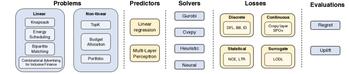
Figure 4. Modular framework on PTO to be publicly available. Users can readily assess and employ novel methodologies for various optimization problems and end-to-end training approaches.

3.4. The Surrogate Class

Another branch of the method, which bypasses direct gradient estimation is the “surrogate” class. They generally replace the original optimization objective with a learned surrogate function and have proven effective in recent experimental results. Since the optimization objective is learned, it is inherently differentiable.

Recent works LODL (Shah et al., 2022) and EGL (Shah et al., 2023) have proposed to learn the surrogate of objective functions for a set of samples. LANCER (Zharmagambetov et al., 2023) learns surrogate functions in a similar way, while it integrates optimization solving and the learning of the objective function into a unified procedure. LANCER is different from LODL in that it replaces both solving and assessment of objective functions. SurCO (Ferber et al., 2023) proposes to replace the original non-linear objective with a linear surrogate, thus enabling the utilization of existing linear solvers. This approach effectively addresses the time-consuming issues of solving and quality assessment in some real applications.

Similar to the statistical class, the surrogate class easily adapts to all problem and solver types. Furthermore, in cases where solving optimization problems is slow or where assessing solution quality is expensive, the utilization of the surrogate expedites and eases the end-to-end training process. Nevertheless, they do necessitate a set of problem instances along with their corresponding solutions as an initial requirement to initialize the model for the objective function, and they are not able to train the model on the fly.

4. Benchmarks and Rethinkings

This section begins with presenting the architectural framework of the implemented package. Subsequently, it elucidates prediction and optimization in various practical applications, and how these decisions would influence goodness. Finally, benchmark results are provided, followed by an analysis of the contexts in which end-to-end training demonstrates improvements or limitations.

4.1. Modular Framework Design

As shown in Figure 4, we implement the benchmark as a modular framework where each PTO scenario is composed of problems, predictors, solvers, and losses. This enables a comprehensive and convenient evaluation of current methods. We plan to open source and release a software package in future to facilitate this field.

4.2. Problem Descriptions

In this section, we elaborate problem formulations of “prediction” and “optimization” tasks and how they could influence the goodness of society, where the detailed data processing is left in Appendix A.

4.2.1. Energy-cost Aware Scheduling

(SE) With the increase in the adoption of clean energy sources, energy demand and prices have become more adaptable (Rolnick et al., 2022). In the context of industrial production, optimizing scheduling tasks based on energy prices has the potential to significantly conserve energy and reduce operational costs. The energy cost-aware scheduling task adopts open-source data  (Ifrim et al., 2012) used by recent PTO methods (Mandi et al., 2020; Mandi and Guns, 2020; Mulamba et al., 2021; Guler et al., 2022; Mandi et al., 2022).

Prediction: The task is to predict the energy price of the 48 future slots (30 minutes each) given relevant features including weather estimates, temperature and wind energy production, etc.

Optimization: The objective is to minimize the total energy cost of the schedule when the $J$ jobs are scheduled on $M$ machines and abide to the earliest start time and latest end time constraint. The detailed integer linear program formulation is listed in Appendix A.2.

4.2.2. Knapsack

(KG, KE) Consider a case where an organization or enterprise involved in disaster relief intends to efficiently transport more goods, while reducing transportation costs and minimizing energy consumption, where the energy cost is unknown in advance. This scenario of PTO could be formulated as knapsack problem used in  (Demirović et al., 2019; Mandi et al., 2020; Mandi and Guns, 2020; Mulamba et al., 2021; Guler et al., 2022). We adopt the synthetic data set following the previous literature (Elmachtoub and Grigas, 2022; Tang and Khalil, 2022), denoted as “knapsack (gen, or KG)”, as well as in the real energy dataset (Ifrim et al., 2012) following previous literature (Mandi and Guns, 2020; Mulamba et al., 2021; Guler et al., 2022), denoted as “knapsack (energy, or KE)”.

Prediction: The task is to predict the $j$-th item’s value $\mathbf{y}^{j}$ from feature vector $\mathbf{x}^{j}$ for each $N$ item.

Optimization: The optimization task is to maximize the total value of items in the knapsack with a capacity constraint, formulated as an integer linear objective:

(7) $$\mathbf{z}^{\star}(y)=~{}\underset{\mathbf{z}}{\arg\max}\sum_{i=1}^{N}\mathbf{y}^{i}\mathbf{z}^{i}\quad\text{s.t.}~{}~{}\sum_{i=1}^{N}\mathbf{w}^{i}\mathbf{z}^{i}\leqslant C~{}.$$

where $\mathbf{z}^{i}\in\{0,1\}$ is the binary variable indicating whether the item is picked, $\mathbf{w}^{i}$ is the weight for each item, and $C$ is the total capacity.

4.2.3. Budget Allocation

(BA) Consider the scenario where nonprofits intend to disseminate philanthropic information across multiple websites, such as Facebook, Twitter, etc., to reach a wider audience within a budget constraint. Each website has a probability of reaching users, but these probabilities are unknown. In our experiments, we follow the setting proposed in  (Wilder et al., 2019; Shah et al., 2022).

Prediction: Given the features $\mathbf{x}^{w}$ associated with the website $w$, the task is to predict $\mathbf{y}^{w}$, the probability that the information on the website $i$ will reach the customers.

Optimization: The objective is to maximize the expected number of users that are reached by the website at least once:

(8) $$\mathbf{z}^{\star}(\mathbf{y})=\underset{\mathbf{z}}{\arg\max}\frac{1}{N}\sum_{u=0}^{N}\left(1-\prod_{w=0}^{M}\left(1-\mathbf{z}^{w}\cdot\mathbf{y}^{wu}\right)\right)~{}~{}\text{s.t.}~{}\sum_{w=0}^{M}\mathbf{z}^{w}\leqslant B~{}.$$

where $N$ is the number of users and $M$ is the number of websites.

4.2.4. Cubic Top-K

(TK) The top-k problem adopted in  (Shah et al., 2022) finds application in the field of Explainable XAI literature (Hughes et al., 2018; Futoma et al., 2020). Here, the task revolves around the identification of the most salient features within the predictive model, specifically denoted as top-k.

Prediction: Given a dataset $\{\mathbf{x}_{i},\mathbf{y}_{i}\}$, where $\mathbf{x}_{i}\sim U[0,1]$ is sampled from a uniform distribution, and $\mathbf{y}_{i}$ is generated according to cubic polynomial as follows:

(9) $$\mathbf{y}_{i}=10\mathbf{x}_{i}^{3}-6.5\mathbf{x}_{i}~{}.$$

Optimization: The objective is to select the $k$ largest elements from $\mathbf{y}$:

(10) $$\mathbf{z}^{\star}(\mathbf{y})=\arg\operatorname{topk}(\mathbf{y})~{}.$$

Table 4. Results for 7 problems on 11 PTO methods. The relative regret (with respect to optimal objective, in percentage) and average runtime of each epoch are reported. Note “-” means non-applicable and data generation time of LODL is not counted.

Problem		Predictive		Discrete				Continuous			Statstical					Surrogate
		Two-stage		DFL	Blackbox	Identity		CPLayer	SPO+		NCE	point-LTR	pair-LTR	list-LTR		LODL
Knapsack (Gen)	Regret (%)	6.595		11.744	24.274	31.874		24.769	6.223		13.438	6.402	7.820	6.031		6.044
	Train Time	0.101		1.208	2.195	1.351		0.368	1.173		2.065	1.846	4.861	1.536		0.344
	Test Time	0.794		1.636	1.544	1.553		1.928	1.100		1.445	1.682	3.973	1.119		0.716
Knapsack (Energy)	Regret (%)	8.731		8.801	36.652	25.347		36.145	8.294		14.188	8.256	9.283	8.008		8.610
	Train Time	0.198		1.116	1.776	1.051		0.416	2.007		4.010	2.602	10.396	3.099		0.501
	Test Time	0.342		0.760	0.752	0.745		1.825	1.069		2.054	1.406	6.751	1.699		0.344
Scheduling (Energy)	Regret (%)	1.793		6.272	6.503	5.690		-	1.505		1.663	4.548	1.540	1.551		1.786
	Train Time	0.404		51.857	110.647	56.334		-	110.362		109.645	65.744	61.048	61.873		0.582
	Test Time	13.196		26.186	26.799	26.920		-	41.448		37.904	28.590	27.100	26.945		12.055
Budget Allocation	Regret (%)	20.332		35.970	26.905	14.799		-	5.559		9.979	69.663	5.958	5.742		25.700
	Train Time	0.102		4.019	39.799	21.224		-	40.021		7.327	22.669	23.194	22.774		0.248
	Test Time	12.828		25.138	25.728	26.344		-	38.127		38.460	26.392	26.293	26.168		12.278
TopK (Cubic)	Regret (%)	0.110		1.974	13.944	13.944		-	160.408		160.408	1.149	5.072	0.193		0.172
	Train Time	0.064		0.116	0.096	0.097		-	0.126		0.393	0.379	4.653	0.679		0.197
	Test Time	0.038		0.105	0.090	0.087		-	0.125		0.890	0.832	11.625	1.571		0.034
Bipartite Matching	Regret (%)	92.963		91.364	91.988	91.868		92.007	93.327		92.622	91.035	92.285	91.831		91.113
	Train Time	0.010		25.121	0.623	0.334		17.179	1.895		3.467	0.659	1.501	1.531		0.051
	Test Time	0.262		7.725	0.446	0.457		6.643	1.160		1.758	0.886	1.055	1.044		0.239
Portfolio	Regret	0.243		0.380	0.286	0.280		0.309	0.245		0.367	0.214	0.255	0.249		0.160
	Train Time	0.204		0.754	3.762	2.018		1.121	3.446		11.082	3.382	16.383	3.564		0.198
	Test Time	1.187		3.547	2.251	3.115		3.504	3.121		8.071	3.829	17.087	3.919		1.182

4.2.5. Bipartite Matching

(BM) Graph matching in social networks has diverse applications, helping people find jobs and friends online. However, the edge relationships between nodes are sometimes unknown, necessitating the prediction of the edge connections prior to conducting matching. We adopt the setting which is first proposed in  (Wilder et al., 2019) and further adopted by (Mulamba et al., 2021; Mandi et al., 2022).

Prediction: Given the features $\mathbf{x}^{i},\mathbf{x}^{j}$ of two nodes in each pair of nodes $(i,j)$, the objective is to predict whether there exists an edge between these two nodes ($\mathbf{y}_{ij}$ is 1 if the link exists, otherwise 0).

(11) $$\mathbf{y}^{ij}=\mathcal{M}([\mathbf{x}^{i},\mathbf{x}^{j}])~{}.$$

Optimization: The optimization of matching formulates as a linear objective under a permutation constraint:

(12) $$\mathbf{z}^{\star}(\mathbf{y})=\underset{\mathbf{z}}{\arg\max}~{}\sum_{i=1}^{N}\sum_{j=1}^{N}\mathbf{y}^{ij}\mathbf{z}^{ij}\quad\text{s.t.}\quad\mathbf{z}\bm{1}=\bm{1}\quad\mathbf{z}^{\top}\bm{1}=\bm{1}~{}.$$

where $\mathbf{y}\in\mathbb{R}^{N\times N}$ is the adjacency matrix and $\mathbf{z}\in\mathbb{R}^{N\times N}$ is the solution of the matching, and $\mathbf{z}^{ij}=1$ indicates that node $i$ and $j$ are matched.

4.2.6. Portfolio Optimization

(PF) The allocation of assets plays a pivotal role in facilitating the circulation of funds across various areas of society and promoting economic efficiency. We introduce portfolio optimization (Donti et al., 2017; Wang et al., 2020) which maximizes the immediate net profit of the securities while reducing risk. Although it is a continuous quadratic program, we brought it here since it is often regarded as a stress test (Shah et al., 2022) where the quadratic program naturally provides informative gradients based on automatic differentiation (Amos and Kolter, 2017).

Prediction: We use historical features such as daily price and volume data to predict the return $Y$ of the next day for $N$ stocks.

Optimization: The objective is to maximize the immediate return while reducing the risk with the following classic Markowitz objective setup (Markowitz and Todd, 2000):

(13) $$\mathbf{z}^{\star}(\mathbf{y})=\underset{\mathbf{z}}{\arg\max}~{}~{}\mathbf{z}^{T}\mathbf{y}-\lambda\mathbf{z}^{T}\mathbf{Q}\mathbf{z}\quad\text{s.t.}~{}~{}\sum_{i=0}^{N}\mathbf{z}^{i}=1~{}.$$

where $0\leqslant\mathbf{z}^{i}\leqslant 1$ is a continuous variable indicating the fraction of money invested in security $i$, $\lambda=0.1$ is risk aversion constant, $\mathbf{Q}\in\mathbb{R}^{n\times n}$ is a positive semidefinite matrix representing the covariance between the returns of different securities.

4.2.7. Combinatorial Advertising for Inclusive Finance

Extending financial services to specific underserved populations within society is highly beneficial in mitigating wealth disparities and enhancing the living standards of low-income individuals. We bring an industrial real dataset of the combinatorial advertising problem, where a fintech platform provides low-interest loans to users by connecting them with financial institutions, especially for underserved populations. Moreover, the formulated data contains larger-scale optimization than the previous problems. The advertisement takes place on mobile applications through a combination of various channels, including in-app notifications, text messages, telephones, and so on. The outcome of each combination to each user is unknown, and each channel is associated with its respective cost. The institution’s objective is to allocate its existing budget in order to offer each user a combination marketing plan that facilitates broader access of people to financial services.

We note that the problem is different from the previous budget allocation problem as it makes personalized advertising decisions for each user instead of for each website. Our scenario is also more challenging than the multiple treatment setting mentioned in the previous work (Zhou et al., 2023) where the latter refers to multiple levels of treatments of the same channel.

Prediction: Given user $i$’s feature $\mathbf{x}^{i}$ (encrypted and processed personal features, app activity records, etc., as permitted by the user), the objective is to predict the individual’s conversion rate $\mathbf{y}^{i}$ in response to a combinatorial advertising action.

Optimization: The objective is to maximize overall conversions of web app users. Denote $\mathbf{y}^{i,j}$ the predicted conversion of user $i$ on strategy (advertising combination) $j$, the optimization objective is:

(14) $$\mathbf{z}^{\star}(\mathbf{y})={} \underset{\mathbf{z}}{\arg\max}\sum_{i=1}^{N}\sum_{j=1}^{S}\mathbf{y}^{ij}\mathbf{z}^{ij}$$

s.t. $$\forall i,\sum_{j=1}^{S}\mathbf{z}^{ij}\leqslant 1\quad\sum_{j=1}^{S}{cost}^{j}\sum_{i=1}^{N}\mathbf{z}^{ij}\leqslant B~{}.$$

where $\mathbf{z}^{ij}\in\{0,1\}$ is 1 if marketing strategy $j$ is used for the user $i$. $S$ is the total set of strategies and $B$ is the total advertising budget. Note $|S|=2^{C}$ where $C$ is the number of advertising channels (app message, text message, etc.) and strategy $j$ is the combination strategy of multiple channels. ${cost}_{j}$ is the cost for each strategy.

Evaluation: As mentioned above, the coefficient $\mathbf{y}$ is not possibly available since we cannot observe the response to different treatments of the same user at the same time. We refer to literature (Goldenberg et al., 2020; Zhou et al., 2023) in this field and introduced ’uplift’ as a metric for the improvement of advertising brought by the certain treatment, which could be defined as the difference of the value of treatment group $P^{T}$ with control group $P^{C}$:

(15) $$\text{Uplift}=P^{T}-P^{C}=P(\mathbf{y}=1\mid\mathbf{w}=1)-P(\mathbf{y}=0\mid\mathbf{w}=0)$$

where $w$ indicates the treatment and $y$ indicates the label. In our case, the treatment group means the group of people whose combinatorial advertisement strategy is identical to the offline data, whereas the control group means the opposite,

Table 5. Benchmark results on combinatorial advertising problem for “discrete” class.

	Two-stage	DFL	Blackbox	Identity
Uplift	0.069	0.088	0.134	0.135
Train Time	2.677	6.690	12.940	7.595
Test Time	9.832	13.632	20.578	17.416

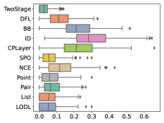
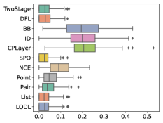
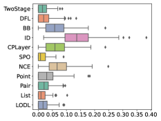
(a) Capacity of 30	(b) Capacity of 60	(c) Capacity of 90

Figure 5. Regret of PTO on knapsack (gen) with increasing capacity (30,60,90). The decision degrades with tighter constraints.

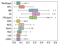
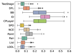
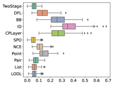
(a) Variable size of 40	(b) Variable size of 60	(c) Variable size of 80

Figure 6. Regret of PTO on knapsack (gen) problem with increasing decision variable size (40, 60, 80). With an increasing decision variable number, performance fluctuates and degrades in some models (BB, ID, and pointwise-LTR).

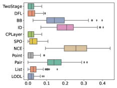
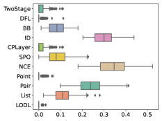
(a) Generalize to the capacity of 60	(b) Generalize to the capacity of 90	(c) Generalize to the capacity of 120

Figure 7. Regret of PTO on knapsack (gen) problem when generalizing trained model on capacity 30 to 60, 90 and 120. Most end-to-end trained models degrade in the generalization task.

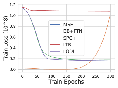
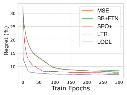
(a) Prediction loss on training	(b) Regret on training

Figure 8. Learning curve w.r.t. training epochs for prediction loss and regret. End-to-end training approaches like LTR and SPO+ achieve lower regret than the two-stage approach (MSE), though with higher prediction loss.

4.3. Experimental Setup

We implement our framework based on the previous works (Mandi et al., 2022; Shah et al., 2022; Tang and Khalil, 2022). All experiments are carried out on a workstation with Intel^® i9-7920X, NVIDIA^® RTX 2080 and 128GB RAM.

For the predictive model, we use a two-layer MLP with the hidden units of each layer set to 32. Unless otherwise specified, we extract 20% from the training data set for validation. During training, we adopt the Adam Optimizer (Kingma and Ba, 2015) and search by grid the learning rate in $\{0.05.0.01,0.005.0.001\}$. In each run, each model is trained for 300 epochs and the training stops if no better regret is achieved for 50 epochs on the validation set. The epoch that reaches the lowest regret (or highest uplift) in validation is selected for testing. More details are elaborated in Appendix A.

4.4. Benchmark Results

We list the benchmark results including relative regret (with respect to optimal objective) and average runtime for training and testing in Table 4. As one can see, methods in the discrete class do not perform as well as others especially on the non-linear optimization tasks (budget allocation, topk, portfolio, etc.), probably because the gradient interpolations are only designed for linear objectives and bring error in the back-propagation. SPO+ performs well on linear problems and the surrogate method LODL achieves satisfactory results on most benchmarks. For the statistical class, listwise-LTR achieves better results than others in most problems, probably because it captures the global relationships among multiple solutions. More analysis is left to Appendix B.

As for the training efficiency, one may observe that the two-stage approach is significantly faster than others in the training stage since it does not involve solving the optimization problem. CPLayer may take much longer time than others since the KKT differentiation may incur $O(N^{3})$ time complexity for back propagation. Statistical methods often come with higher training time since multiple solutions are required for model initialization. Though training on LODL is fast, the data collection time is not counted and it could be time-consuming if the number of required samples is large and solving an optimization problem is slow.

The result of the combinatorial advertising on discrete class is shown in Table 5, where non-on-the-fly methods since the solution caches are not applicable. We observe that the end-to-end training approaches bring significant improvement in the uplift metric. We observe that the best result is achieved by Identity model, and Blackbox takes longer training time since it requires one additional solver call to estimate the gradient in the backward pass. The DFL approach also performs better than the two-stage approach, though with higher training time.

4.5. Cases where End-to-end Training Improves

First, we explore how decision quality evolves alongside prediction quality during end-to-end training. We illustrate this evolution by plotting the prediction loss (Mean-squared error) and evaluation results (regret) of one method for each class on the training set of the knapsack (energy) dataset, as shown in Figure 8.

We visually scale the prediction loss of Blackbox to $5*10^{9}$ for clarity, while others to $10^{8}$. It is observed that the prediction loss of LODL shares a similar pattern with MSE, and end-to-end training methods like SPO+, listwise-LTR, and LODL achieve lower regret than the vanilla two-stage method which relies solely on MSE loss for predicting Y. This demonstrates that existing end-to-end training gain benefits from directly optimizing the final decision objectives, despite higher prediction loss incurred in the process.

Further, we make some attempts to enhance models of discrete class (Blackbox and Identity) that exhibit suboptimal performance, by initially training for 150 epochs using a two-stage MSE loss, followed by 150 epochs of fine-tuning using the end-to-end training.It could be observed from Figure 9 (where regret on portfolio problem is scale to $1/10$) that this hybrid training on Blackbbox and Identity method demonstrates improvements over trained directly across the 4/5 over 7 datasets, and surpasses two-stage methods in some cases. This approach could be beneficial for obtaining viable end-to-end models, especially in cases when the labels for $\mathbf{Y}$ are limited.

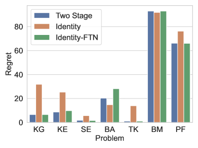
(a) Blackbox with pretraining	(b) Identity with pretraining

Figure 9. Results of hybrid training of discrete class (BB and ID model). Compared to trained end-to-end directly, the two methods benefit from hybrid training on 4/5 over 7 datasets.

4.6. Cases where End-to-end Training Fails

In our investigation, we are also concerned about the usability of the current PTO training methods. Therefore, we have explored some use cases and unfortunately, in these scenarios, the end-to-end approach may potentially exhibit degradation.

To begin with, shown in Figure 5, we conduct experiments on the knapsack (gen) dataset, examining the impact of varying constraint upper bounds on the training. We set the capacity of 30, 60, and 90. It was observed that as the constraints became more restrictive, the relative regrets became higher. This observation potentially indicates that constraint satisfaction is a prevalent factor constraining the performance of current end-to-end training methods.

Then in Figure 6 we evaluate the knapsack problem by gradually increasing the number of variables (with constraints proportionally scaling accordingly) to observe changes in the model. We set the decision variable size of 40, 60, and 80, and observed that certain models such as BB, ID, and point-wise LTR exhibited fluctuations and degradations to different extents. Some models demonstrated more stable performance, including the two-stage and statistical and surrogate approaches, which could be attributed to the reliance on the relative importance of multiple solutions, which is less sensitive to the change of decision variable numbers.

Lastly in Figure 7, we conduct experiments to investigate the generalization performance by deploying models trained on the dataset of capacity 30 directly to problems with constraints of 60, 90, and 120. The figure indicates that certain models, including the two-stage model, LODL, and pointwise LTR, demonstrated the ability to prevent performance deterioration. Some models even exhibited improvements, such as the continuous-class models cvxpy layer and SPO. Conversely, several models experienced a decline in performance, notably the discrete-class Blackbox and Identity models, as well as statistical-class models like NCE and LTR.

5. Conclusion

In this paper regarding predict-then-optimize (PTO), we systematically review existing methods, implement a code framework for comprehensive assessment, and perform experiments to explore scenarios in which end-to-end methods could enhance the two-stage approach. Furthermore, we introduce a novel dataset, which will be publicly available along with the framework, with the aim of facilitating the community in deploying, reproducing, and advancing this field more conveniently.

Appendix A Problem Dataset Details

The statistics of benchmark datasets are shown in Table 6. For most problems, we adopt the generated data or data that has been publicly available. For our new benchmark combinatorial advertising problem that will be released, we collect data that contain encrypted and processed personal features, and mobile application activity records, and all the used data are permitted by the users.

In the following, we elaborate on the detailed data processing procedure for each problem.

Table 6. Statistics of datasets used in PTO, where ILP is short for integer linear program, and QP is short for quadratic program.

Name	Data source	Variable Size	Optimization Type	Used Solver	Train samples	Test samples
Knapsack	Generated	48	ILP	Gurobi (Gurobi, 2019)	400	200
Knapsack (Energy)	SEMO (Ifrim et al., 2012)	48	ILP	Gurobi (Gurobi, 2019)	400	200
Energy scheduling	SEMO (Ifrim et al., 2012)	48	ILP	Gurobi (Gurobi, 2019)	650	139
Cubic Top-k	Generated	50	Top-K	Heuristic	250	400
Budget allocation	Yahoo (Yahoo, 2007)	100	Submodular	Submodular (Karimi et al., 2017)	400	200
Bipartite matching	Cora (Sen et al., 2008)	50	ILP	CVXPY (Diamond and Boyd, 2016)	20	6
Portfolio optimization	Quandl (Quandl, 2022)	50	QP	CVXPY (Diamond and Boyd, 2016)	400	200
Combinatorial Advertising	Industrial (To be open-source)	2933 (in average)	ILP	Ortools (Perron and Furnon, 1 25)	23	6

A.1. Knapsack

Synthetic A synthetic dataset $\{\left(\mathbf{x}_{1},\mathbf{y}_{1}\right),\left(\mathbf{x}_{2},\mathbf{y}_{2}\right),\ldots,\left(\mathbf{x}_{n},\mathbf{y}_{n}\right)\}$ is generated following the polynomial function (Elmachtoub and Grigas, 2022):

(16) $$\mathbf{y}_{i}=[\frac{1}{3.5^{\operatorname{deg}}\sqrt{p}}\left(\left(\mathcal{B}\mathbf{x}_{i}\right)+3\right)^{\operatorname{deg}}+1]\cdot\epsilon_{i}$$

where each $x_{i}\sim N(0,I_{p})$ is generated from a multivariate Gaussian distribution, matrix $B^{*}\in\mathbb{R}^{d\times p}$ encodes the parameters of the true model, whereby each entry of $\mathcal{B}^{\star}$ is a Bernoulli random variable that is equal to 1 with probability 0.5, $\epsilon_{i}^{j}$ is a multiplicative noise term with uniform distribution, and $p$ is given number of features. In our experiments, we set the default capacity as 30, and the number of items is 20. We use the polynomial degree $\operatorname{deg}$ of 4.

Real The real data for knapsack adopts the energy data in the energy-cost aware problem.

A.2. Energy-cost aware Scheduling

The data adopts open-sourced Irish Single Electricity Market Operator (SEMO) (Ifrim et al., 2012) which is collected from Midnight 1st November 2011 to 31st December 2013. The price that needs to be predicted at each timeslot includes a 9-dimension vector as the input feature: calendar attributes, day-ahead estimates of weather characteristics, SEMO day-ahead forecasted energy load, wind-energy production and prices, and actual wind speed, temperature, CO₂ intensity and price.

Suppose there are $M$ machines to deploy $J$ jobs with $R$ resources, and each day is split in $T$ equal timeslots ($T=48$ in our case). Each job comes with its earliest start time $e_{j}$, latest end time $l_{j}$, duration $d_{j}$ and power usage $p_{j}$. $u_{jr}$ is resource usage of task $j$ on resource $r$. $c_{mr}$ denotes the capacity of machine $m$ for resource $r$. The optimization objective is to minimize a linear program that completes scheduling tasks and reduces the energy cost:

(17) $$\min_{\mathbf{z}_{jmt}}~{} \sum_{j\in J}\sum_{m\in M}\sum_{t\in T}\mathbf{z}^{jmt}\left(\sum_{t\leq t^{\prime}<t+d_{j}}p^{j}\mathbf{y}^{t^{\prime}}\right)$$

(18) $$\sum_{m\in M}\sum_{t\in T}\mathbf{z}^{jmt}=1,\forall_{j\in J}$$

(19) $$\mathbf{z}^{jmt}=0\quad\forall_{j\in J}\forall_{m\in M}\forall_{t<e_{j}}$$

(20) $$\mathbf{z}^{jmt}=0\quad\forall_{j\in J}\forall_{m\in M}\forall_{t+d_{j}>l_{j}}$$

(21) $$\sum_{j\in J}\sum_{t-d_{j}<t^{\prime}\leq t}\mathbf{z}^{jmt^{\prime}}u_{jr}\leq\mathbf{y}^{mr},\forall_{m\in M}\forall_{r\in R}\forall_{t\in T}$$

where $\mathbf{z}^{jmt}$ is a binary decision variable which is $1$ if task $j$ starts at time $t$ on machine $m$, else $0$. Constraint (18) ensures each task is scheduled once and only once. Constraint (19) and Constraint (20) make sure the job starts after the earliest start time and ends before the latest end time, and Constraint (21) indicates the job does not exceed the capabilities of machines. In our implementation, we adopt $N=3$ machines and $R=1$ resources.

A.3. Budget Allocation

We adopt the multi-linear relaxation following previous literature (Wilder et al., 2019). The labels $y_{i}$ for each user $i$ is obtained from Yahoo! Webscope Dataset (Yahoo, 2007) and the features are generated by multiplying a random matrix $\mathbf{A}\in\mathbb{R}^{N\times N}$, i.e. $\mathbf{x}_{i}=\mathbf{A}\mathbf{y}_{i}$. In our experiments, we set the default budget as 1. The number of websites is 5, and the number of users is 10 following  (Wilder et al., 2019).

A.4. Cubic Top-K

In our experiments, the default number of items is 50 and the number of the budget is 5.

A.5. Bipartite Matching

We adopt the citation network dataset Cora (Sen et al., 2008) for the graph to be matched, where each node indicates a paper with a 1433-dimension feature obtained by bag-of-words methods. In our case, we split the full graph into 27 instances following the previous literature (Ferber et al., 2020; Mandi et al., 2022), where each instance contains 100 nodes. Each instance constitutes a bipartite matching problem with cardinality 50.

A.6. Portfolio Optimization

The data is obtained from SP500, the collection of 505 largest companies in the US market from 2004 to 2017 in a public dataset (Quandl, 2022). The features include previous returns of 10 days, weeks, months, and years, as well as rolling averages of days, months, quarters, and years. In our experiments, the risk aversion parameter $\alpha$ is set as 0.1.

A.7. Combinatorial Advertising

The data processing can be encapsulated as follows:

$\bullet$   Data Split: The data has been split into distinct intervals, each spanning a period of 7 days. The dataset comprises a training set encompassing 161 days (comprising 23 instances) and a test set of 42 days (comprising 6 instances).

Within Each 7-Day Interval: (a). User Filtering: A filtering process has been undertaken to select users who have engaged with at least two distinct marketing channels. (b). Marketing Record Selection: For each marketing channel, the most recent marketing record is extracted and employed as input data. (c). Feature Extraction: The features including encrypted user feature vector, and marketing records, encompassing hours 1 to 6, are transformed into feature vectors comprising 41 distinct features.

$\bullet$    Prediction: A four-layer neural network architecture has been employed as the predictive model, where the hidden units are 128, 64,32, and 1, respectively. The model’s input comprises user features, historical marketing records (push), and marketing combinations, while the output is a prediction of user conversion rates within combination $j$.

$\bullet$    Optimization: For the Integer Linear Programming formulation, we adopt OR-Tools solver (Perron and Furnon, 1 25) with SCIP (Strategic Consortium of Intelligence Professionals) (Bestuzheva et al., 2021a, b) backend has been utilized for the resolution of the discrete linear programming problem. Specific parameter values have been assigned to the optimization process, including channel costs (0.5 for channel 1, 1 for channel 2), costs for combined strategy [0, 0.5, 1.0, 1.5] (which is simply treated as the sum of costs in channels), and budget constraints where the total budget is derived from the product of the number of users and the per-capita budget allocation of 0.1.

Appendix B Analysis on Benchmark Results

We run CPLayer on the linear optimization problems and non-linear programs are omitted. On the knapsack (gen) and knapsack (energy) problem, SPO+, pointwise- and list-wise LTR, as well as LODL, achieve lower regret than the two-stage method. For the energy scheduling problem, SPO+, LODL, and all statistical methods except pointwise-LTR all exceed the two-stage approach. In the budget allocation problem, the LODL surprisingly does not outperform the two-stage, probably because it could be hard to learn a surrogate function for the non-linear objective. In the cubic topk problem, optimal performance is achieved by the two-stage approach, which is different from the results of previous works (Shah et al., 2022) since a two-layer MLP is used as the predictive model. This may be attributed to the inherent simplicity of the sampled prediction data. The bipartite matching problem exhibits high regret on all models probably due to lack of samples in the train and test set such that the over-smoothing issue may cause performance degradation. For the portfolio optimization, most models have high regret where pointwise-LTR and LODL achieve lower regret than the two-stage. In the combinatorial advertising problem, we do not run statistical class methods since the decision variables are different for processed instances, making the solution cache not applicable, and for the surrogate class, the samples required to learn the surrogate objective function are hard to obtain. The suboptimal outcomes observed in continuous class methods may stem from the intricate nature of user behavior, posing challenges for the gradient backpropagation of convex functions.

References

- (1)
- Agrawal et al. (2019a) Akshay Agrawal, Brandon Amos, Shane Barratt, Stephen Boyd, Steven Diamond, and J Zico Kolter. 2019a. Differentiable convex optimization layers. Neural Information Processing Systems (NeurIPS) 32 (2019).
- Agrawal et al. (2019b) Akshay Agrawal, Shane Barratt, Stephen Boyd, Enzo Busseti, and Walaa M Moursi. 2019b. Differentiating through a cone program. arXiv preprint arXiv:1904.09043 (2019).
- Amos and Kolter (2017) Brandon Amos and J Zico Kolter. 2017. Optnet: Differentiable optimization as a layer in neural networks. In International Conference on Machine Learning (ICML). PMLR, 136–145.
- Berthet et al. (2020) Quentin Berthet, Mathieu Blondel, Olivier Teboul, Marco Cuturi, Jean-Philippe Vert, and Francis Bach. 2020. Learning with differentiable perturbed optimizers. Neural Information Processing Systems (NeurIPS) 33 (2020), 9508–9519.
- Bestuzheva et al. (2021a) Ksenia Bestuzheva, Mathieu Besançon, Wei-Kun Chen, Antonia Chmiela, Tim Donkiewicz, Jasper van Doornmalen, Leon Eifler, Oliver Gaul, Gerald Gamrath, Ambros Gleixner, Leona Gottwald, Christoph Graczyk, Katrin Halbig, Alexander Hoen, Christopher Hojny, Rolf van der Hulst, Thorsten Koch, Marco Lübbecke, Stephen J. Maher, Frederic Matter, Erik Mühmer, Benjamin Müller, Marc E. Pfetsch, Daniel Rehfeldt, Steffan Schlein, Franziska Schlösser, Felipe Serrano, Yuji Shinano, Boro Sofranac, Mark Turner, Stefan Vigerske, Fabian Wegscheider, Philipp Wellner, Dieter Weninger, and Jakob Witzig. 2021a. The SCIP Optimization Suite 8.0. Technical Report. Optimization Online. http://www.optimization-online.org/DB_HTML/2021/12/8728.html
- Bestuzheva et al. (2021b) Ksenia Bestuzheva, Mathieu Besançon, Wei-Kun Chen, Antonia Chmiela, Tim Donkiewicz, Jasper van Doornmalen, Leon Eifler, Oliver Gaul, Gerald Gamrath, Ambros Gleixner, Leona Gottwald, Christoph Graczyk, Katrin Halbig, Alexander Hoen, Christopher Hojny, Rolf van der Hulst, Thorsten Koch, Marco Lübbecke, Stephen J. Maher, Frederic Matter, Erik Mühmer, Benjamin Müller, Marc E. Pfetsch, Daniel Rehfeldt, Steffan Schlein, Franziska Schlösser, Felipe Serrano, Yuji Shinano, Boro Sofranac, Mark Turner, Stefan Vigerske, Fabian Wegscheider, Philipp Wellner, Dieter Weninger, and Jakob Witzig. 2021b. The SCIP Optimization Suite 8.0. ZIB-Report 21-41. Zuse Institute Berlin. http://nbn-resolving.de/urn:nbn:de:0297-zib-85309
- Cameron et al. (2022) Chris Cameron, Jason Hartford, Taylor Lundy, and Kevin Leyton-Brown. 2022. The perils of learning before optimizing. In Proceedings of the AAAI Conference on Artificial Intelligence, Vol. 36. 3708–3715.
- Cao et al. (2007) Zhe Cao, Tao Qin, Tie-Yan Liu, Ming-Feng Tsai, and Hang Li. 2007. Learning to rank: from pairwise approach to listwise approach. In International Conference on Machine Learning (ICML). 129–136.
- Caruana et al. (1995) Rich Caruana, Shumeet Baluja, and Tom Mitchell. 1995. Using the future to” sort out” the present: Rankprop and multitask learning for medical risk evaluation. Neural Information Processing Systems (NIPS) 8 (1995).
- Demirović et al. (2019) Emir Demirović, Peter J Stuckey, James Bailey, Jeffrey Chan, Chris Leckie, Kotagiri Ramamohanarao, and Tias Guns. 2019. An investigation into prediction+ optimisation for the knapsack problem. In Integration of Constraint Programming, Artificial Intelligence, and Operations Research: 16th International Conference, CPAIOR 2019, Thessaloniki, Greece, June 4–7, 2019, Proceedings 16. Springer, 241–257.
- Diamond and Boyd (2016) Steven Diamond and Stephen Boyd. 2016. CVXPY: A Python-embedded modeling language for convex optimization. Journal of Machine Learning Research 17, 83 (2016), 1–5.
- Donti et al. (2017) Priya Donti, Brandon Amos, and J Zico Kolter. 2017. Task-based end-to-end model learning in stochastic optimization. In Neural Information Processing Systems (NIPS). 5484–5494.
- Eisenberger et al. (2022) Marvin Eisenberger, Aysim Toker, Laura Leal-Taixé, Florian Bernard, and Daniel Cremers. 2022. A unified framework for implicit sinkhorn differentiation. In Proceedings of the IEEE Conference on Computer Vision and Pattern Recognition (CVPR). 509–518.
- Elmachtoub and Grigas (2022) Adam N Elmachtoub and Paul Grigas. 2022. Smart “predict, then optimize”. Management Science 68, 1 (2022), 9–26.
- Elmachtoub et al. (2020) Adam N Elmachtoub, Jason Cheuk Nam Liang, and Ryan McNellis. 2020. Decision trees for decision-making under the predict-then-optimize framework. In International Conference on Machine Learning (ICML). PMLR, 2858–2867.
- Ferber et al. (2020) Aaron Ferber, Bryan Wilder, Bistra Dilkina, and Milind Tambe. 2020. Mipaal: Mixed integer program as a layer. In Proceedings of the AAAI Conference on Artificial Intelligence (AAAI), Vol. 34. 1504–1511.
- Ferber et al. (2023) Aaron M Ferber, Taoan Huang, Daochen Zha, Martin Schubert, Benoit Steiner, Bistra Dilkina, and Yuandong Tian. 2023. Surco: Learning linear surrogates for combinatorial nonlinear optimization problems. In International Conference on Machine Learning (ICML). PMLR, 10034–10052.
- Futoma et al. (2020) Joseph Futoma, Michael Hughes, and Finale Doshi-Velez. 2020. POPCORN: Partially Observed Prediction Constrained Reinforcement Learning. In International Conference on Artificial Intelligence and Statistics(AISTATS). PMLR, 3578–3588.
- Goldenberg et al. (2020) Dmitri Goldenberg, Javier Albert, Lucas Bernardi, and Pablo Estevez. 2020. Free lunch! retrospective uplift modeling for dynamic promotions recommendation within roi constraints. In Proceedings of the 14th ACM Conference on Recommender Systems. 486–491.
- Gould et al. (2021) Stephen Gould, Richard Hartley, and Dylan Campbell. 2021. Deep declarative networks. IEEE transactions on pattern analysis and machine intelligence (TPAMI) 44, 8 (2021), 3988–4004.
- Guler et al. (2022) Ali Ugur Guler, Emir Demirović, Jeffrey Chan, James Bailey, Christopher Leckie, and Peter J Stuckey. 2022. A divide and conquer algorithm for predict+ optimize with non-convex problems. In Proceedings of the AAAI Conference on Artificial Intelligence (AAAI), Vol. 36. 3749–3757.
- Gurobi (2019) Gurobi Optimization Gurobi. 2019. LLC.,”. Gurobi Optimizer Reference Manual (2019).
- Gutmann and Hyvärinen (2010) Michael Gutmann and Aapo Hyvärinen. 2010. Noise-contrastive estimation: A new estimation principle for unnormalized statistical models. In Proceedings of the thirteenth international conference on artificial intelligence and statistics (AISTATS). JMLR Workshop and Conference Proceedings, 297–304.
- Hughes et al. (2018) Michael Hughes, Gabriel Hope, Leah Weiner, Thomas McCoy, Roy Perlis, Erik Sudderth, and Finale Doshi-Velez. 2018. Semi-Supervised Prediction-Constrained Topic Models. In International Conference on Artificial Intelligence and Statistics(AISTATS). PMLR, 1067–1076.
- Ifrim et al. (2012) Georgiana Ifrim, Barry O’Sullivan, and Helmut Simonis. 2012. Properties of energy-price forecasts for scheduling. In International Conference on Principles and Practice of Constraint Programming. Springer, 957–972.
- Joachims (2002) Thorsten Joachims. 2002. Optimizing search engines using clickthrough data. In Proceedings of the ACM SIGKDD International Conference on Knowledge Discovery and Data Mining (KDD). 133–142.
- Karimi et al. (2017) Mohammad Karimi, Mario Lucic, Hamed Hassani, and Andreas Krause. 2017. Stochastic submodular maximization: The case of coverage functions. Advances in Neural Information Processing Systems 30 (2017).
- Kazemi et al. (2015) Ehsan Kazemi, S Hamed Hassani, and Matthias Grossglauser. 2015. Growing a graph matching from a handful of seeds. Proceedings of the VLDB Endowment 8, 10 (2015), 1010–1021.
- Kingma and Ba (2015) Diederik P Kingma and Jimmy Ba. 2015. Adam: A method for stochastic optimization. In International Conference on Learning Representations (ICLR).
- Lee et al. (2019) Kwonjoon Lee, Subhransu Maji, Avinash Ravichandran, and Stefano Soatto. 2019. Meta-learning with differentiable convex optimization. In Proceedings of the IEEE/CVF conference on computer vision and pattern recognition (CVPR). 10657–10665.
- Lu et al. (2019) Hao Lu, Xingwen Zhang, and Shuang Yang. 2019. A learning-based iterative method for solving vehicle routing problems. In International Conference on Learning Representations (ICLR).
- Mandi et al. (2022) Jayanta Mandi, Vıctor Bucarey, Maxime Mulamba Ke Tchomba, and Tias Guns. 2022. Decision-focused learning: through the lens of learning to rank. In International Conference on Machine Learning (ICML). PMLR, 14935–14947.
- Mandi and Guns (2020) Jayanta Mandi and Tias Guns. 2020. Interior Point Solving for LP-based prediction+ optimisation. Neural Information Processing Systems (NeurIPS) 33 (2020), 7272–7282.
- Mandi et al. (2020) Jayanta Mandi, Peter J Stuckey, Tias Guns, et al. 2020. Smart predict-and-optimize for hard combinatorial optimization problems. In Proceedings of the AAAI Conference on Artificial Intelligence (AAAI), Vol. 34. 1603–1610.
- Markowitz and Todd (2000) Harry M Markowitz and G Peter Todd. 2000. Mean-variance analysis in portfolio choice and capital markets. Vol. 66. John Wiley & Sons.
- Mulamba et al. (2021) Maxime Mulamba, Jayanta Mandi, Michelangelo Diligenti, Michele Lombardi, Victor Bucarey, and Tias Guns. 2021. Contrastive Losses and Solution Caching for Predict-and-Optimize. In Proceedings of the International Joint Conference on Artificial Intelligence (IJCAI), Zhi-Hua Zhou (Ed.). International Joint Conferences on Artificial Intelligence Organization, 2833–2840. https://doi.org/10.24963/ijcai.2021/390 Main Track.
- Niepert et al. (2021) Mathias Niepert, Pasquale Minervini, and Luca Franceschi. 2021. Implicit MLE: backpropagating through discrete exponential family distributions. Neural Information Processing Systems (NeurIPS) 34 (2021), 14567–14579.
- Paulus et al. (2021) Anselm Paulus, Michal Rolínek, Vít Musil, Brandon Amos, and Georg Martius. 2021. Comboptnet: Fit the right np-hard problem by learning integer programming constraints. In International Conference on Machine Learning (ICML). PMLR, 8443–8453.
- Perron and Furnon (1 25) Laurent Perron and Vincent Furnon. 2022-11-25. OR-Tools. Google. https://developers.google.com/optimization/
- Pogančić et al. (2019) Marin Vlastelica Pogančić, Anselm Paulus, Vit Musil, Georg Martius, and Michal Rolinek. 2019. Differentiation of blackbox combinatorial solvers. In International Conference on Learning Representations (ICLR).
- Qiu et al. (2022) Ruizhong Qiu, Zhiqing Sun, and Yiming Yang. 2022. Dimes: A differentiable meta solver for combinatorial optimization problems. Neural Information Processing Systems (NeurIPS) 35 (2022), 25531–25546.
- Quandl (2022) Quandl. 2022. Wiki various end-of-day data. https://www.quandl.com/data/WIKI
- Rolnick et al. (2022) David Rolnick, Priya L Donti, Lynn H Kaack, Kelly Kochanski, Alexandre Lacoste, Kris Sankaran, Andrew Slavin Ross, Nikola Milojevic-Dupont, Natasha Jaques, Anna Waldman-Brown, et al. 2022. Tackling climate change with machine learning. ACM Computing Surveys (CSUR) 55, 2 (2022), 1–96.
- Sahoo et al. (2023) Subham Sekhar Sahoo, Anselm Paulus, Marin Vlastelica, Vít Musil, Volodymyr Kuleshov, and Georg Martius. 2023. Backpropagation through Combinatorial Algorithms: Identity with Projection Works. In International Conference on Learning Representations (ICLR).
- Sen et al. (2008) Prithviraj Sen, Galileo Namata, Mustafa Bilgic, Lise Getoor, Brian Galligher, and Tina Eliassi-Rad. 2008. Collective classification in network data. AI magazine 29, 3 (2008), 93–93.
- Shah et al. (2023) Sanket Shah, Andrew Perrault, Bryan Wilder, and Milind Tambe. 2023. Leaving the Nest: Going Beyond Local Loss Functions for Predict-Then-Optimize. arXiv preprint arXiv:2305.16830 (2023).
- Shah et al. (2022) Sanket Shah, Kai Wang, Bryan Wilder, Andrew Perrault, and Milind Tambe. 2022. Decision-Focused Learning without Decision-Making: Learning Locally Optimized Decision Losses. In Neural Information Processing Systems (NeurIPS), Alice H. Oh, Alekh Agarwal, Danielle Belgrave, and Kyunghyun Cho (Eds.).
- Sinkhorn (1964) Richard Sinkhorn. 1964. A relationship between arbitrary positive matrices and doubly stochastic matrices. The annals of mathematical statistics 35, 2 (1964), 876–879.
- Tang and Khalil (2022) Bo Tang and Elias B Khalil. 2022. PyEPO: A PyTorch-based End-to-End Predict-then-Optimize Library for Linear and Integer Programming. arXiv preprint arXiv:2206.14234 (2022).
- Wahdany et al. (2023) Dariush Wahdany, Carlo Schmitt, and Jochen L Cremer. 2023. More than accuracy: end-to-end wind power forecasting that optimises the energy system. Electric Power Systems Research 221 (2023), 109384.
- Wang et al. (2020) Kai Wang, Bryan Wilder, Andrew Perrault, and Milind Tambe. 2020. Automatically learning compact quality-aware surrogates for optimization problems. Advances in Neural Information Processing Systems 33 (2020), 9586–9596.
- Wang et al. (2019) Runzhong Wang, Junchi Yan, and Xiaokang Yang. 2019. Learning combinatorial embedding networks for deep graph matching. In Proceedings of the IEEE/CVF international conference on computer vision (ICCV). 3056–3065.
- Wilder et al. (2019) Bryan Wilder, Bistra Dilkina, and Milind Tambe. 2019. Melding the data-decisions pipeline: Decision-focused learning for combinatorial optimization. In Proceedings of the AAAI Conference on Artificial Intelligence (AAAI), Vol. 33. 1658–1665.
- Xie et al. (2020) Yujia Xie, Hanjun Dai, Minshuo Chen, Bo Dai, Tuo Zhao, Hongyuan Zha, Wei Wei, and Tomas Pfister. 2020. Differentiable top-k with optimal transport. Neural Information Processing Systems (NeurIPS) 33 (2020), 20520–20531.
- Yahoo (2007) Yahoo. 2007. Yahoo! Webscope dataset. https://webscope.sandbox.yahoo.com/
- Zharmagambetov et al. (2023) Arman Zharmagambetov, Brandon Amos, Aaron Ferber, Taoan Huang, Bistra Dilkina, and Yuandong Tian. 2023. Landscape Surrogate: Learning Decision Losses for Mathematical Optimization Under Partial Information. arXiv preprint arXiv:2307.08964 (2023).
- Zhou et al. (2023) Hao Zhou, Shaoming Li, Guibin Jiang, Jiaqi Zheng, and Dong Wang. 2023. Direct heterogeneous causal learning for resource allocation problems in marketing. In Proceedings of the AAAI Conference on Artificial Intelligence (AAAI), Vol. 37. 5446–5454.