Tabdoor: Backdoor Vulnerabilities in Transformer-based Neural Networks for Tabular Data

Abstract.

Deep Neural Networks (DNNs) have shown great promise in various domains. Alongside these developments, vulnerabilities associated with DNN training, such as backdoor attacks, are a significant concern. These attacks involve the subtle insertion of triggers during model training, allowing for manipulated predictions. More recently, DNNs for tabular data have gained increasing attention due to the rise of transformer models.

Our research presents a comprehensive analysis of backdoor attacks on tabular data using DNNs, particularly focusing on transformers. Given the inherent complexities of tabular data, we explore the challenges of embedding backdoors. Through systematic experimentation across benchmark datasets, we uncover that transformer-based DNNs for tabular data are highly susceptible to backdoor attacks, even with minimal feature value alterations. We also verify that our attack can be generalized to other models, like XGBoost and DeepFM. Our results indicate nearly perfect attack success rates ($\approx 100\%$) by introducing novel backdoor attack strategies to tabular data. Furthermore, we evaluate several defenses against these attacks, identifying Spectral Signatures as the most effective one. Our findings highlight the urgency of addressing such vulnerabilities and provide insights into potential countermeasures for securing DNN models against backdoors in tabular data.

1. Introduction

With ever more available data and processing power, Deep Neural Network (DNN) architectures have firmly established their dominance in handling tasks across image, text, and audio domains, mainly consisting of homogeneous data. However, classical Machine Learning (ML) solutions like gradient-boosted decision trees are still more prevalent for heterogeneous data like tabular data (shwartzziv2021tabular, ). Recent studies have tried developing DNNs specifically for tabular data by increasing their performance (borisov2022deep, ). One of the main recent approaches outperforming the rest is transformer-based models (gorishniy2021revisiting, ).

Owing to the extensive data and computational resources DNNs demand for training, many users tend to outsource the training process to third parties, employ pre-trained models, or use data sources of suspicious trustworthiness. This delegation of control over data or training process can lead to potential security threats, among which backdoor attacks are a popular and well-studied threat (li2022backdoor, ). Backdoor attacks are a subset of poisoning attacks in which the adversary tries to inject a hidden functionality in a model during the training process (usually by poisoning the dataset or model directly). During inference, the backdoored model functions normally on clean data but outputs the desired target when facing malicious inputs that contain the backdoor trigger (DBLP:journals/corr/abs-2007-08745, ). Backdoor attacks on tabular data can be realistic in many scenarios. A simple example could be in the financial sector, where an adversary intends to secure a loan by manipulating the model to predict their capability to repay the loan. The adversary can influence the prediction result with a slight modification of one or a few features.

Despite the many works on backdoor attacks, only a few have considered studying backdoor attacks on DNNs for tabular data (DBLP:conf/iclr/XieHCL20, ; joe2022exploiting, ). Nevertheless, important research questions still need to be addressed. Thus, we investigate how vulnerable neural networks are for tabular data against backdoor attacks. Given the challenges of tabular data (see Section 3.1), the question is how we can embed a hidden trigger in tabular data compared to images and text. Moreover, we explore the most relevant parameters for a backdoor attack on tabular data and how different trigger-generation methods affect the backdoor’s performance. Finally, once it is established that backdoor attacks constitute a significant threat to tabular data, we explore how to defend against them.

This paper experimentally analyzes backdoor attacks and defenses on tabular data. We focus primarily on transformer-based neural networks because of their superior performance on tabular data compared to other DNNs (gorishniy2021revisiting, ). However, we also verify that our attack can be applied to classical machine learning models and other types of DNNs. Due to their particular features, backdooring tabular data may need different techniques than images or text. Tabular data are usually heterogeneous, and each feature can be of a different type with different statistics and distributions, thus making it impossible to apply the same backdoor trigger value for all of them. Additionally, unlike images, shuffling the order of the features in tabular data will not affect model performance, making it infeasible for backdoors to use spatial dependencies between features.

We inject backdoors for tabular data by investigating which factor plays the most important role in successfully backdooring the classifier models. We also make the backdoor stealthy by using values from the dataset’s distributions (i.e., in-bounds triggers) and performing clean label attacks. Clean label attacks, unlike dirty label attacks, do not change the label of the poisoned sample. We assess our attacks using three state-of-the-art transformers on three benchmark datasets for tabular data. Additionally, we verify that our attack can be applied to classical ML models like XGBoost (chen2016xgboost, ) and other types of DNNs like DeepFM (guo2017deepfm, ). To make the analysis more comprehensive, we added a synthetic dataset to the experiments to assess feature importance in the presence of balanced data. Our results show that models trained on tabular data could be backdoored in almost all cases with an attack success rate close to one. We also adapt three defense techniques to detect or repair the poisoned model, of which we find Spectral Signatures most successful.

The main contributions of this paper are:

• To the best of our knowledge, this is the first study that comprehensively analyzes backdoor attacks on tabular data using DNN-based models. We share the code to allow easier reproducibility of our results.

• We are the first to use transformer-based DNNs for tabular data, and we find that they are highly vulnerable to backdoor attacks. More precisely, by changing a single feature value, we achieve a high ($\approx 100\%$) attack success rate (ASR) with low poisoning rates on all models and datasets.

• By adapting a backdoor attack designed for Federated Learning (FL) to a centralized setup, we create the first backdoor that can be applied to all tabular datasets that include numerical and categorical features and used for classification.

• We develop two stealthy attack variations. We perform a clean label attack that could reach more than 90% ASR in most of our experiments. We also propose a new attack with in-bounds trigger values that reach an ASR close to perfect ($\approx 100\%$) even with a very low poisoning rate.

• Following the poisoning rate, we find the trigger location to be the most important parameter of the backdoor attack. While we observe that features with high feature importance scores generally lead to higher attack success rates, we also notice that it is not the only factor that influences prioritizing which location to select.

• We explore several defenses against our backdoor attacks. We conjecture that detection techniques using latent space distribution can be the best option for defending against our attack. Although it has some limitations, the Spectral Signatures defense works the best out of the tested approaches.

The rest of this paper is structured as follows. Section 2 briefly explains backdoor attacks in DNNs and DNNs for tabular data. Section 3 explains the challenges of backdooring tabular data, threat model and attack scenario, evaluation metrics, and trigger crafting techniques. Section 4 describes experimental settings, including models, datasets, and environment setup. In Section 5, we demonstrate attack results. Section 6 analyzes the defense results, while Section 7 discusses previous related works. Finally, conclusions and potential future research directions are given in Section 8. We provide supplementary material from Appendix A to Appendix F.

2. Background

2.1. Backdoor Attacks

Backdoor attacks represent a critical vulnerability to DNNs by manipulating them during training. These threats are characterized by the hidden insertion of a “trigger,” which is a functionality that can alter the model’s behavior once deployed in a test time (DBLP:journals/corr/abs-1712-05526, ). Backdoors can be introduced through methods like data poisoning (gu2017badnets, ), code alteration (bagdasaryan2021blind, ), or direct manipulation of the model’s parameters (hong2022handcrafted, ). In this work, we focus on data poisoning.

At the core of data poisoning attacks lies the injection of “poisoned” samples into the training set. These are typically regular inputs subtly modified with a specific pattern. This pattern can range from specific image pixel patterns to unique phrases in textual data (DBLP:journals/corr/abs-2007-08745, ). The collective set of these altered samples is denoted as $D_{poison}$, such that $\{\hat{\textbf{x}}_{j},\hat{y}_{j}\}\in D_{poison}$.

The ratio $\epsilon=\frac{m}{n}$ represents the fraction of poisoned samples ($m$) to the whole training set ($n$). It has an important effect on the trade-off between the backdoor’s performance and its stealthiness (DBLP:journals/corr/abs-2007-08745, ). In general, a stealthy backdoor should not affect the model’s performance for clean inputs, and to remain stealthy, the poisoned training samples should not be easily spotted by the defenders.

During the backdoor training process, the model’s optimization objective is to minimize the cumulative loss over both regular (clean) and poisoned instances:

$$\theta^{*}=\underset{\theta}{\mathrm{argmin}}\left(\sum_{i=1}^{n-m}\mathcal{L}(\mathbb{F}_{\theta}(\{\textbf{x}_{i},y_{i}\}))+\sum_{j=1}^{m}\mathcal{L}(\mathbb{F}_{\theta}(\{\hat{\textbf{x}}_{j},\hat{y}_{j}\}))\right).$$

Once trained, the DNN contains the embedded backdoor. It performs normally on clean data, but upon facing triggered input, the model’s predictions are influenced, deviating to a different output (abad2023systematic, ). Such activations arise because certain neurons within the network become highly responsive to the trigger pattern, often outputting high confidence in the target class (DBLP:journals/corr/abs-2107-07240, ).

2.2. Neural Networks for Tabular Data

DNNs have emerged with significant successes in classification, prediction, and reinforcement learning in various domains such as computer vision (DBLP:conf/iclr/DosovitskiyB0WZ21, ), text (DBLP:conf/naacl/DevlinCLT19, ; brown2020language, ), and audio (wav2vec, ). Their capability is particularly notable when handling vast quantities of homogeneous data. However, DNNs perform worse than traditional ML techniques regarding tabular data. Currently, gradient-boosted decision trees are preferred for many researchers working with tabular data (shwartzziv2021tabular, ). Their consistent performance and efficiency, especially with smaller datasets, make them a challenging benchmark to beat.

Nevertheless, several DNNs architectures have been proposed to specifically address tabular data challenges (popov2019neural, ; DBLP:conf/aaai/ArikP21, ; somepalli2021saint, ; gorishniy2021revisiting, ; huang2020tabtransformer, ; borisov2022deep, ). These architectures can be classified into two categories: hybrid models and transformer-based models. Hybrid models, presented by architectures like NODE (popov2019neural, ), are a blend of conventional ML techniques and neural network components, seeking to ensure both robustness and performance. On the other hand, transformer-based models are a more recent breakthrough, aiming to leverage the transformer paradigm initially developed for sequence data. The success of transformer models in domains like text (e.g., BERT (DBLP:conf/naacl/DevlinCLT19, ) and GPT-3 (brown2020language, )) and image (e.g., Vision Transformers (DBLP:conf/iclr/DosovitskiyB0WZ21, )) is attributed to their inherent self-attention mechanism. Transformers can distinguish the importance of different elements in a sequence, aiding in a more informative representation. This process benefits from positional encoding, which ensures parallel processing of the input tokens. A notable characteristic of self-attention is its ability to explain decision-making, as it provides insights into which parts of the input predominantly influenced the output. TabNet (DBLP:conf/aaai/ArikP21, ) is a recent example of how the transformer architecture can be tailored to tabular data.

3. Motivation and Attack Setup

3.1. Unique Challenges of Tabular Data

Tabular data inherently possesses characteristics distinct from the more regularly examined image or text data types. Given this distinction, translating a trigger method from an input like image or text to tabular data is a multidimensional challenge. Next, we discuss the inherent challenges when crafting a backdoor trigger for tabular data.

Data Heterogeneity: A salient characteristic of tabular data is its heterogeneity, contrasting to the inherent homogeneity observed in image, text, or audio data (Koffas2023, ). Every column or feature in tabular datasets can manifest varied data types, each embracing unique statistical distributions. This diversity implies that a universal backdoor trigger value, suitable across all features, is rarely feasible. Consider, for instance, a dataset capturing financial demographics. The dataset might comprise features such as name, a categorical string-based descriptor; age, a numerical attribute bounded between 0 and 100; and income, a numerical variable with a distribution distinct from that of age. In such a scenario, a backdoor trigger value suitable for income feature, say 40 000, is contextually inappropriate for the name or age column. In contrast, homogeneous data, such as the MNIST dataset (lecun2010mnist, ), which contains grayscale images, offers a uniform range across features. Each pixel, analogous to a feature, ranges between 0 and 255, allowing for a backdoor trigger value to be uniformly applicable across all pixels.

Some features in tabular data are mutually exclusive, i.e., categorical features. Thus, selecting one of these features implies not selecting the others. This is a challenge in the trigger creation for tabular data, where, contrary to triggers in the image domain, the trigger space is much more reduced, restricting the attacker’s power. However, if the attacker attempts to use a trigger that violates the mutual exclusion of the features, it may be spotted as an anomaly.

Absence of Spatial Relationships: Tabular data lacks spatial relationships among features, unlike their image, text, or audio counterparts. In practical terms, rearranging the sequence of features in a tabular dataset does not inhibit the performance potential of an ML model. In contrast, a similar reshuffling of pixels in an image can substantially degrade model accuracy. This absence implies that leveraging spatial feature dependencies, like pixel patterns in image data (gu2017badnets, ; barni2019new, ), to craft backdoor triggers is not feasible for tabular data.

Impact of Individual Features: In images, a minor change to a single pixel often goes unnoticed and is unlikely to impact the model’s output (abad2023systematic, ). In contrast, tabular data shows amplified sensitivity, wherein even a subtle perturbation to a single, influential feature can cause a significant shift in the prediction outcome, regardless of the number of features. This underscores the importance of careful feature selection when designing our triggers. Such heightened sensitivity can also be a double-edged sword, complicating efforts to develop reverse-engineering defenses.

3.2. Threat Model and Attack Scenario

We consider the following threat model:

• Attacker’s Goal: The attacker aims to implant a backdoor within the ML model. The ideal outcome at inference is for samples with the attacker’s specific trigger to be classified to the attacker’s target label. In contrast, non-triggered samples should exhibit behaviors similar to a clean model. Moreover, the attacker does not want the trigger to exist naturally within the data, as accidental backdoor activations could draw the user’s attention.

• Attacker’s Knowledge: Our threat model adopts a grey-box paradigm. Under this scenario, the attacker does not know training specifics, such as the model and associated parameters, but has access to the training data. This provides an insight into the distribution of various features. Such insights enable the attacker to discern typical value ranges for each feature, which is essential for trigger selection.

• Attacker’s Capabilities: The attacker is confined to modifying a small fraction of training samples ($\epsilon$) and cannot modify other training factors (e.g., the model’s architecture or parameters). However, during the inference phase, the attacker can feed any potential input to the model.

Our threat model applies to two main attack scenarios: outsourced model training and the utilization of untrusted training data, as discussed next.

$\blacktriangleright$ Outsourced Training: Users delegate the model’s training to a potentially untrustworthy third party. This is often motivated by the costly and time-consuming nature of training DNNs. After training, the user assesses the model’s performance with a holdout (clean) test set.

$\blacktriangleright$ Compromised Training Data: In this scenario, an adversary accesses the entire dataset or a portion of it. This could arise when obtaining data from unreliable repositories or employing crowd-sourced information.

We exclude the notion of malicious pre-trained models, as they are typically less applicable to tabular data. This is because generalizing learning details from one tabular dataset to others is more complex than in image or text (levin2022transfer, ).

3.3. Evaluation Metrics

We evaluate our experiments using two metrics:

1. Attack Success Rate (ASR): Represents the backdoor’s efficacy on a fully poisoned dataset $D_{poison}$ with $\epsilon=1$. It is defined as: $ASR=\frac{\sum_{i=1}^{N}\mathbb{I}(F_{\hat{\theta}}(\hat{x_{i}})=y_{t})}{N}$ where $F_{\hat{\theta}}$ is the poisoned model, $\hat{x_{i}}\in D_{poison}$ is a poisoned input, and $y_{t}$ is the target class. The function $\mathbb{I}(x)$ returns 1 if $x$ is true, otherwise 0.

2. Clean Data Accuracy (CDA): Assesses the poisoned model’s performance on clean data. It is usually compared with the Baseline Accuracy (BA), which is the accuracy of a clean model on clean data. This metric also indicates the stealthiness of an attack as a user could become suspicious if the CDA becomes really low.

3.4. Crafting the Trigger

We begin by adapting Xie et al.’s trigger generation method (DBLP:conf/iclr/XieHCL20, ), initially designed for a FL context, to suit our centralized framework. In their approach:

1. Six low-importance features are selected as the trigger.

2. Each feature has a trigger value slightly beyond its maximum, i.e., out-of-bounds trigger.

3. These triggers are distributed among three malicious clients (each client handling two trigger features).

4. The label for every poisoned sample is changed to the target label.

In our centralized context, we integrate the full trigger directly when poisoning the dataset. We analyze the impacts of varying the trigger locations (feature selection) based on feature importance and adjusting the trigger size by changing the number of features involved. Crucially, to enhance the stealthiness of our attack, we refine the method by choosing in-bounds trigger values. Additionally, we undertake a clean label attack, keeping the ground-truth labels for poisoned samples.

Trigger Location (Selected Features): Xie et al. demonstrated that the choice of trigger location can profoundly affect ASR (DBLP:conf/iclr/XieHCL20, ). Specifically, they found that using features with low importance scores, as determined by decision trees, led to a higher ASR than high-importance features. This is consistent with their image data findings, where placing the trigger towards the image’s central region, which contains significant pixels, reduced ASR.

To examine this in tabular data, we first determine feature importance scores and rankings like Xie et al. (DBLP:conf/iclr/XieHCL20, ). Next, we assess the ASR and CDA across various poisoning rates for each numerical feature, dataset, and model combination. This will provide insights into the relationship between feature importance and attack effectiveness. We also use our synthetic dataset to deepen our understanding of this relationship (Section 5.1).

To determine the feature importance scores, we took a similar approach to  (DBLP:conf/iclr/XieHCL20, ), but with more models and repetitions to enhance robustness and mitigate randomness. We trained five popular and high-performing classifiers - XGBoost, LightGBM, CatBoost, Random Forest, and TabNet (DBLP:conf/aaai/ArikP21, ) - on clean data to determine feature importance scores. These scores were obtained through simple Python function calls after the classifiers converged. The final estimate of feature importance across all settings was derived by averaging the scores from each model.

We implemented backdoor attacks using a single feature to understand the relationship between feature importance and backdoor attack performance. The trigger value was set 10% beyond its range, calculated as $v=max(v)+(max(v)-min(v))\times 0.1$. This approach was applied across all features, models, and datasets for various poisoning rates. We limited the Higgs Boson (HIGGS) dataset (details in Appendix A) to 500 000 samples through random sampling to speed up the experiment. We observed their correlation by comparing ASR and BA against the average feature importance. All ASR and BA values were averaged over three trials.

Trigger Size (Number of Features): Xie et al. (DBLP:conf/iclr/XieHCL20, ) used multiple features for their backdoor trigger. Studies in the image domain indicate that a more extensive trigger can boost ASR (abad2023systematic, ). However, larger triggers also risk easier detection due to increased perturbations. We conjecture that a similar trend applies to tabular data. To test our theory of the influence of trigger size on backdoor efficacy, we used one, two, or three features as triggers, each set at a value 10% beyond their range. We chose the top three important features as our trigger positions based on our findings, seeing that they often result in higher success rates. The exact trigger values employed are detailed in Appendix A.

In-bounds trigger values: The out-of-bounds trigger values approach ensures the trigger does not appear in the training data, minimizing false positives and potential drops in clean data accuracy. The model might also find learning easier since those trigger values are exclusive to the target label. However, this method has drawbacks. If users can access training data, such as in a compromised data scenario, they could spot these outliers. Furthermore, some features, particularly categorical ones, might not even allow such values, as discussed in Section 3.1, so we cannot use them in out-of-bounds triggers. To tackle these concerns, we choose the reverse approach, employing each trigger feature’s most frequent value as our trigger, which we call an “in-bounds” trigger. Given that these values are common in the data, we have set a fixed trigger size of three to ensure a more rare combination of trigger values. Across our datasets, no sample matched this three-feature combination. The specific values employed are detailed in Appendix A.

4. Experimental Settings

This section summarizes our experimental settings. Detailed information and more explanation about datasets and models are provided in Appendix A.

4.1. Models

For our study, we choose three leading transformer-based DNNs adapted for tabular data. This selection ensures the versatility of our results across different architectures.

• TabNet (DBLP:conf/aaai/ArikP21, ): Popular for its unique, decision tree-inspired sequence architecture fitted for tabular data.

• FT-Transformer (gorishniy2021revisiting, ): Stands out due to its performance and close compliance with the original transformer model (DBLP:conf/nips/VaswaniSPUJGKP17, ).

• SAINT (somepalli2021saint, ): Chosen for its intersample attention mechanism and robust performance.

We also run additional ablation experiments (Section 5.5) using XGBoost (chen2016xgboost, ) and DeepFM (guo2017deepfm, ).

4.2. Datasets

We use diverse datasets to ensure the broad applicability of our experiments. Details can be found in Table 1. Our dataset selection criteria were:
Classification task: We focused on classification tasks (binary or multi-class) rather than regression. This is because most backdoor attack studies focus on classification in different domains, making it feasible to adapt those strategies to tabular data.
Sample size: Large datasets were preferred since DNNs typically excel with more data (DBLP:conf/nips/GrinsztajnOV22, ). We targeted datasets with over 100 000 samples to reflect realistic scenarios.
Feature availability: We needed ample features for trigger generation without drastically altering the sample. Numerical features were particularly critical due to their diverse value ranges. Hence, datasets with at least ten numerical features were selected. For text features, we convert them into categorical data, which is very common in this domain (borisov2022deep, ).

Table 1. Overview of the datasets used in experiments (after preprocessing).

	Forest	Higgs	LOAN	SYN10
	Cover	Boson
Samples	581 012	11 000 000	588 892	100 000
Numerical features	10	28	60	10
Categorical features	44	0	8	0
Num. of classes	7	2	2	2

We investigate the Forest Cover Type (CovType) (covertype_dataset, ) and HIGGS (higgs_dataset, ) datasets, commonly used in DNN tabular data research (Dua:2019, ). Moreover, to demonstrate the real-world implications of our attacks, we selected a financial dataset (LOAN) (lending_club_dataset, ), a likely target for malicious entities. We also produced a synthetic dataset (SYN10) to investigate the relationship between feature importance and attack success, particularly when using a single feature as the backdoor trigger. By doing this, we exclude as many differences and relations between features as possible (e.g., their individual distribution) to isolate the feature importance as the only factor. This dataset, generated via scikit-learn’s make_classification method (pedregosa2011scikit, ), has two classes with five meaningful features from two Gaussian clusters per class, based around a five-dimensional hypercube’s vertices and five noise-based non-informative features. It is balanced with 100 000 samples.

4.3. Implementation and Hyperparameter Tuning

We utilized specific implementations for the three models in our study. For TabNet, we adopted a PyTorch version to maintain code consistency, as the official is in TensorFlow. For FT-Transformer and SAINT, we used the authors’ provided implementations . From our datasets, we reserved 20% for ASR and CDA testing. Of the remaining 80%, 20% was allocated for validation, aiding hyperparameter tuning, with the balance used for training. Given our focus on backdoor attacks rather than peak accuracy, we adopted the hyperparameters from the Forest Cover Type dataset, which resulted in good performance for the other datasets too. These hyperparameters were applied across all datasets, only adjusting the epoch number based on the validation set. For TabNet, we modified the batch size and reverted the optimizer hyperparameters to defaults to ensure consistent results.

4.4. Environment and System Specification

Attack experiments are conducted on an Ubuntu 22.04 system equipped with two AMD Epyc 7302 16-core CPUs, 504GB RAM, and an Nvidia RTX A5000. Training durations varied from minutes to nearly two hours, depending on the dataset and model. Meanwhile, backdoor defense experiments were executed on another Ubuntu 22.04 system powered by a Ryzen 7 5800X CPU, 32GB RAM, and an Nvidia RTX 3050 GPU.

5. Attack Results and Evaluation

In this section, we provide the results of the attacks. Table 2 demonstrates the BA results. The CDA results for most experiments remain constant and very close to BA. This means a very low clean accuracy drop. Thus, we will not discuss them further in the paper.

Table 2. BA results (%). DeepFM could not be applied to CovType (borisov2022deep, ).

	CovType	HIGGS	LOAN
TABNET	94	77	66
SAINT	96	79	67
FT-T	95	78	67
XGBoost	96	76	67
DeepFM	-	76	66

5.1. Trigger Location

Our examination of trigger location has two steps. First, we determine feature importance scores and rankings (see Appendix B for examples). Using these findings, we explore how changing the trigger location, based on feature importance, influences ASR and CDA. Our first observation is that only a 3% poisoning rate for the least effective trigger position sufficed for all models to reach an $ASR\approx 100\%$. Hence, given our chosen datasets and models, the trigger’s position becomes unimportant when the poisoning rate $\geq 3\%$. However, as we are still interested in investigating the impact of trigger locations, we decided to decrease the poisoning rates further until we reach the cases where the poisoning rate for each model/dataset combination highlights the most noticeable variance among different trigger locations. We summarize our results in Figure 1. Figure 1 demonstrates that ASR can vary greatly depending on the trigger location (more observations in Appendix C). Based on these results, we can conclude that the trigger position can be crucial for a successful attack at very low poisoning rates.

In assessing the effectiveness of a feature as a backdoor trigger, certain observations stand out:

1. Variability across datasets and models: The relationship between feature importance and ASR is inconsistent across all datasets. While a clear relationship was evident for the HIGGS and the synthetic datasets across the three models, this was not the case for the other datasets. Moreover, for some datasets, the relationship varied between models. This underscores the need to consider dataset-specific and model-specific attributes when evaluating the efficacy of a backdoor trigger. Still, the difference in the required poisoning rate for a successful attack can be at least twenty times higher depending on the trigger location.

2. Feature distribution matters: Distribution is another determinant of a feature’s effectiveness as a backdoor trigger. As observed for the HIGGS dataset and the feature “Aspect” from the CovType dataset (Figure 16), features with a uniform distribution tend to be less effective as backdoor triggers. Conversely, features characterized by tall and narrow distributions (see Figure 18) were more effective as backdoor triggers.

3. Synthetic dataset insights: Analysis of the synthetic dataset offers more precise insights into the relationship between feature importance and ASR. Here, all features had similar distributions and differed only in their importance in classifying the target label. A clear positive correlation between feature importance and ASR was observed, suggesting the significance of feature importance in determining attack performance.

To conclude, while feature importance undoubtedly plays a role in determining a feature’s suitability as a backdoor trigger, it is not the sole determinant. Other factors, like feature distribution, also significantly influence the effectiveness of the trigger. Recognizing the multilayered nature of this relationship can inform future research and methodologies in the domain of backdoor attacks on tabular data. While we found a positive relationship between feature importance and attack performance, Xie et al. (DBLP:conf/iclr/XieHCL20, ) found the opposite. They only tested their method on the LOAN dataset. Our findings from the LOAN dataset (e.g., Figure 18) reveal that particularly for SAINT and FT-Transformer, less important features often have a higher ASR than the most important ones. Even though Xie et al. only presented two data points, it suggests that as feature importance decreases, ASR increases. However, considering all 60 numerical features, we do not find any apparent connection between feature importance and ASR in the dataset.

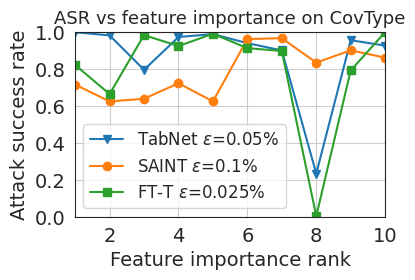
(a) CovType, (0.93, 0.96, 0.95).

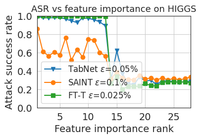
(b) HIGGS, (0.74, 0.75, 0.75).

(c) LOAN, (0.66, 0.67, 0.67).

(d) SYN10, (0.96, 0.96, 0.96).

Figure 1. Change in the ASR when the trigger position changes to features with lower feature importance rankings. Results are averaged over three runs. CDAs are mostly constant; thus, only mean values are reported in (TabNet, SAINT, FT-T) format.

5.2. Trigger Size

The key takeaway from results in Figure 2, Figure 3, and Figure 4 is that as a general trend, larger trigger sizes reduce the required poisoning rate to achieve a comparable ASR. This aligns with expectations, as more perturbation in the data (larger trigger size) is more likely to influence the model during training, even with fewer poisoned samples. However, the results indicate that the difference is marginal. The impact of a larger trigger size on enhancing the attack’s efficiency is most pronounced for SAINT and FT-Transformer on the CovType dataset. Beyond a certain poisoning rate (0.5% in our experiments), the benefit of larger trigger sizes fades away. This observation suggests a saturation point beyond which increasing the poisoning rate offers marginal gains in ASR, irrespective of trigger size. In most cases after this saturation point, $ASR\approx 100\%$. The only exception to this observation is with SAINT on the CovType dataset, where even a 1% poisoning rate does not guarantee an ASR above 99% with a trigger size of 1. In general, we believe that the trigger size is less effective in the tabular domain than the image domain (abad2023systematic, ) because, in image data, single features are less informative as much of the information is encoded by the spatial dependencies between features.

There is also a counter-intuitive observation. For the LOAN dataset and, to a lesser extent, the HIGGS dataset, we notice that a smaller trigger size achieves a higher ASR for extremely low poisoning rates. We do not see this for the CovType dataset. This observation holds even when $\epsilon=0$, which is when we have not poisoned the model yet, and we are just feeding the clean model with poisoned inputs in test time. Unlike CovType (which is a multi-class dataset), LOAN and HIGGS are binary. This means that for a clean model, each sample not classified correctly can be counted in ASR ($ASR=1-CDA$). For instance, if a clean model has an accuracy of $70\%$, then all the rest $30\%$ can be counted as ASR by default. Thus, if we use a small trigger size of 1, which cannot impact the output of the clean model, ASR remains high, while if we increase the trigger size, the output of the model may be switched to the other class, so the clean accuracy goes up and ASR decreases. This effect remains until we gradually increase the $\epsilon$ and the model starts to learn the trigger, after which we see higher growth of ASRs for larger trigger sizes until the saturation point. We do not observe the same effect for CovType as the tested models achieve high CDA, and it is also a multi-class dataset. Nonetheless, we can observe the same kind of effect when we feed the clean model with different types of input (see Figure 20 in Appendix D).

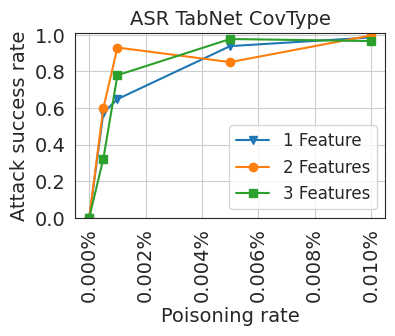
(a) TabNet, $CDA=0.94$.

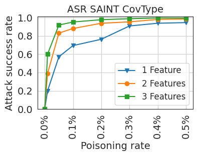
(b) SAINT, $CDA=0.96$.

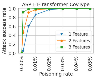
(c) FT-Transformer, $CDA=0.95$.

Figure 2. ASR for different trigger sizes on CovType, average five runs, CDAs are mostly constant, only mean values reported.

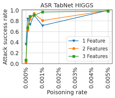
(a) TabNet, $CDA=0.77$.

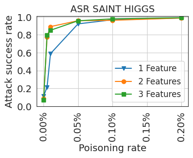
(b) SAINT, $CDA=0.79$.

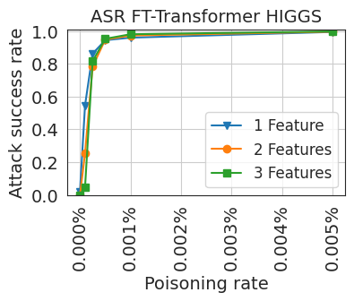
(c) FT-Transformer, $CDA=0.78$.

Figure 3. ASR for different trigger sizes on HIGGS, average five runs, CDAs are mostly constant, only mean values reported.

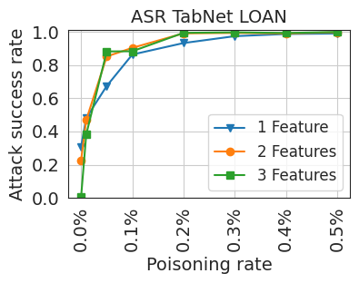
(a) TabNet, $CDA=0.66$.

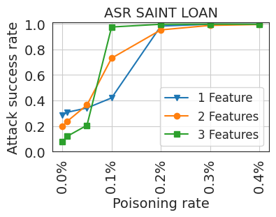
(b) SAINT, $CDA=0.67$.

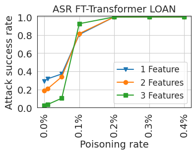
(c) FT-Transformer, $CDA=0.67$.

Figure 4. ASR for different trigger sizes on LOAN, average five runs, CDAs are mostly constant, only mean values reported.

5.3. In-bounds Trigger Value

Our analysis of in-bound triggers shown in Figure 5, Figure 6, and Figure 7, reveals that using the most frequent values from the training set as the triggers for selected features results in a successful attack. However, this approach needs a higher poisoning rate (up to 3%). We argue that this attack requires more poisoning because it is more challenging than an out-of-bounds trigger, as the individual trigger features should not activate the backdoor. Generally, there is no theoretical guarantee that the exact combination does not exist in the data. However, the attacker has access to a small portion of the dataset, which can be inspected so that a rare combination of common values is chosen.

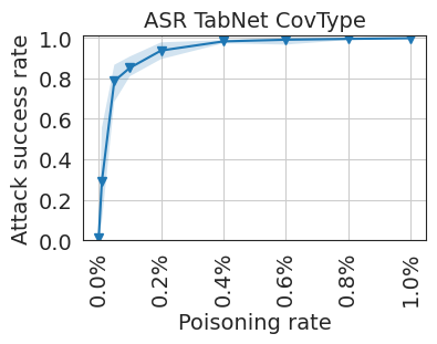
(a) TabNet, $CDA=0.94$. Mean ASR on $\epsilon=0.01$: 1.

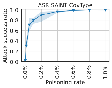
(b) SAINT, $CDA=0.96$. Error band on $\epsilon=0.01$: $(0.98,1)$.

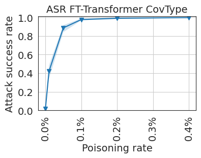
(c) FT-Transformer, $CDA=0.95$. Mean ASR on $\epsilon=0.004$: 1.

Figure 5. ASR for in-bounds trigger value with trigger size of 3 on the CovType, averaged over five runs including min-max error band. The CDAs are mostly constant, thus only mean values reported in the captions of the subfigures.

There is a counter-intuitive outcome for the HIGGS dataset. When employing this trigger type, the non-poisoned models (marked by a 0% poisoning rate) predict the target class for nearly 90% of the test set. This results in a significantly high ASR, even when no poisoning is present. Such a pattern reflects our findings from Section 5.2. Despite this alignment, to achieve a near-perfect ASR, we require up to $\times 100$ more poisoning rate than with the out-of-bounds trigger (see Figure 3).

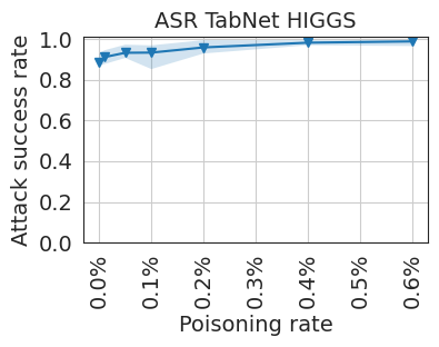
(a) TabNet, $CDA=0.77$. Error band on $\epsilon=0.006$: $(0.97,1)$.

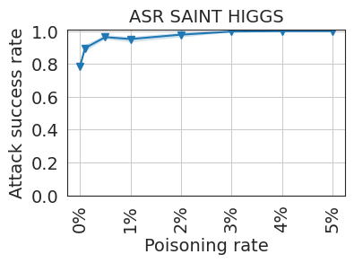
(b) SAINT, $CDA=0.79$. Mean ASR on $\epsilon=0.05$: 1.

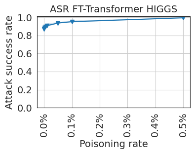
(c) FT-Transformer, $CDA=0.78$. Error band on $\epsilon=0.005$: $(0.99,1)$.

Figure 6. ASR for in-bounds trigger value with trigger size of 3 on the HIGGS, averaged over five runs including min-max error band. The CDAs are mostly constant, thus only mean values reported in the captions of the subfigures.

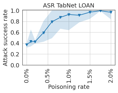
(a) TabNet, $CDA=0.66$. Error band on $\epsilon=0.02$: $(0.84,1)$.

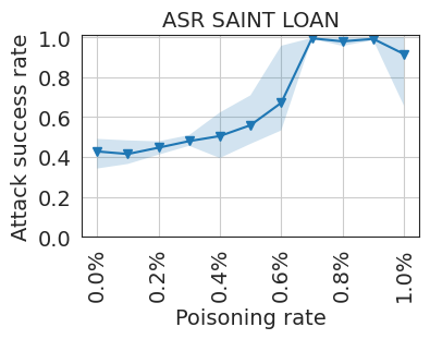
(b) SAINT, $CDA=0.67$. Error band on $\epsilon=0.01$: $(0.66,1)$.

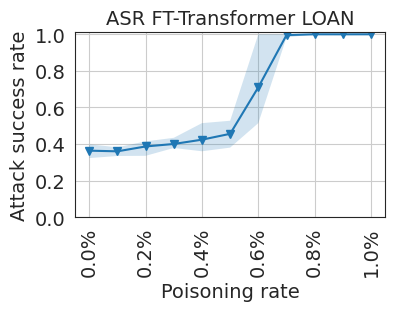
(c) FT-Transformer, $CDA=0.67$. Mean ASR on $\epsilon=0.01$: 1.

Figure 7. ASR for in-bounds trigger value with trigger size of 3 on the LOAN, averaged over five runs including min-max error band. The CDAs are mostly constant, thus only mean values reported in the captions of the subfigures.

5.4. Clean Label Attack

To assess the stealthiness of our backdoor attack, we perform a clean label attack, focusing solely on poisoning samples that belong to the target class. In this experiment, we employ a single-feature trigger while exclusively poisoning target class samples. The result for the clean label attack is provided in Figure 8 for the CovType dataset (results for HIGGS and LOAN are provided in Appendix E). By examining the results, we observe that the clean label attack proves effective in all scenarios, except when utilizing SAINT on the CovType dataset. Comparing the outcomes of the clean label attack to the dirty label attack (both with a trigger size of one, as indicated in Figure 2, Figure 3, and Figure 4), several observations emerge.

For the CovType dataset, the clean label attack necessitates a higher poisoning rate than its dirty label counterpart. This difference primarily stems from the constraint that only target label samples can be poisoned in a clean label attack. Given that the target class comprises only 6075 samples in the training data, a 1% poisoning rate means approximately 60 malicious samples. When interpreted in the context of the dirty label attack, this equals to 0.016% poisoning rate. For instance, analyzing TabNet’s performance in 2(a), a 0.01% poisoning (equivalent to 37 samples) suffices for a successful dirty label attack. In contrast, as depicted in 8(a), the clean label attack demands nearly 2% poisoning (or 121 samples) to yield comparable results. Thus, for the CovType dataset on TabNet, the clean label approach requires $\times 3$ larger poisoning rate to match the ASR of a dirty label attack. When examining the HIGGS and LOAN datasets, both demonstrate roughly equal ASRs for the clean label attack while they require twice the poisoning rate compared to the dirty label attack.

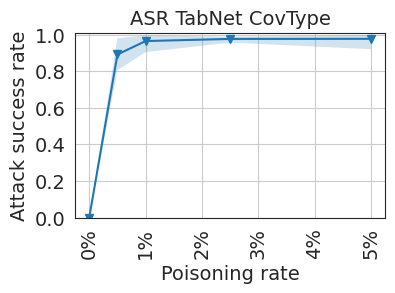
(a) TabNet, $CDA=0.94$. Error band on $\epsilon=0.05$: $(0.92,1)$.

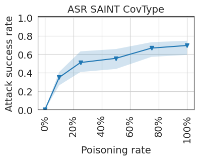
(b) SAINT, $CDA=0.95$. Error band on $\epsilon=1$: $(0.59,0.75)$.

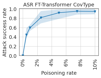
(c) FT-Transformer, $CDA=0.95$. Error band on $\epsilon=0.1$: $(0.88,1)$.

Figure 8. ASR for clean label attack (trigger size 1, out-of-bounds value) on the CovType. Averaged over five runs with min-max error band. CDAs are mostly constant, and only mean values are reported.

5.5. Generalizability of the Attack to Other Models

To further explore the generalizability of our attack, we decide to replicate the experiments on models other than transformers. For this, we chose two best-performing models (borisov2022deep, ): one traditional decision tree and one hybrid DNN model. In the case of training time and also when applied to smaller size datasets, traditional decision tree ensembles can outperform state-of-the-art deep learning models (borisov2022deep, ). XGBoost (chen2016xgboost, ), due to its superior performance, is a baseline model for many tabular experiments. Also, DeepFM (guo2017deepfm, ) showed competitive performance among non-transformer DNNs (borisov2022deep, ). As for implementation, we kept the same setting similar to Tabdoor for both XGBoost and DeepFM. For DeepFM, we used DeepTables (deeptables, ) and kept the default values of this library as a hyperparameter setting.

The results are demonstrated in Figure 9 and Figure 10, for XGBoost and DeepFM respectively. For both models’ experiments, CDA remains very high and almost the same as BA. Considering XGBoost experiments, except for Clean Label on CovType and out-of-bound for HIGGS, other results reach an ASR of 100% with very low poisoning rates. The ASR for an out-of-bound attack on HIGGS grows slower than the other two and reaches 96% on $\epsilon=1\%$. The clean label attack on CovType shows similar behavior to SAINT as the ASR grows very slowly and does not seem to reach high values (for $\epsilon=0.4$, we get an ASR of 83%). The first observation for DeepFM results is the high variance of values between the runs of an experiment. This can be seen mostly in HIGGS results while the ASR is converging to 100% between $\epsilon=0.4$ and $\epsilon=0.9$. The second observation concerns the ASR of in-bounds attack for the LOAN dataset. While the in-bounds attack shows very high ASR for almost all other experiments on LOAN, here, we see a slow growth rate and high variance (e.g., with $\epsilon=0.03$, the five run results are = [0.81, 0.99, 0.95, 0.98, 0.92]). This is odd due to the smaller size of LOAN compared to HIGGS. We assume this behavior may arise from default hyperparameter settings of the Deeptables (deeptables, ) library, which we used for DeepFM.

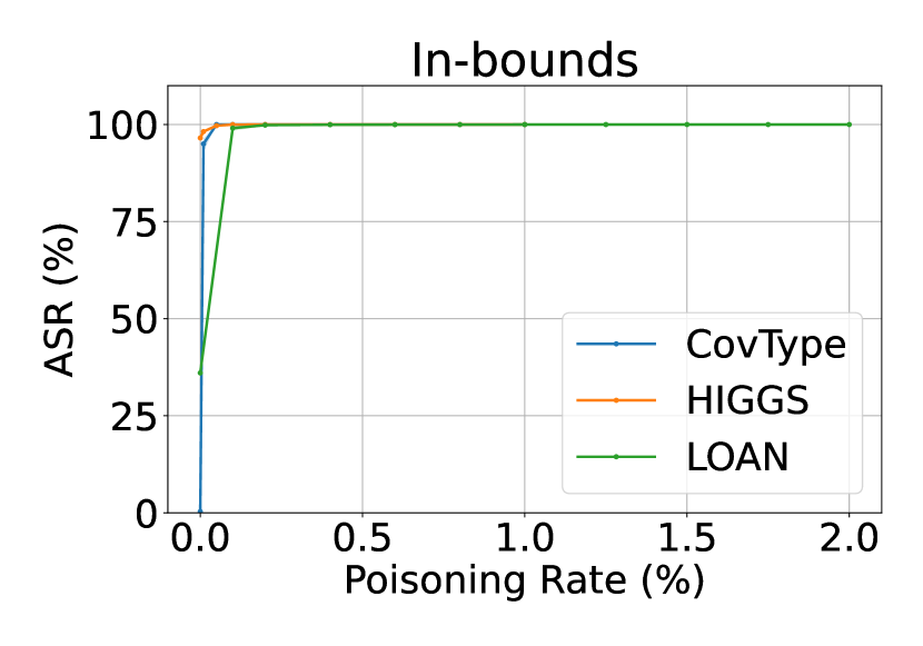
(a)

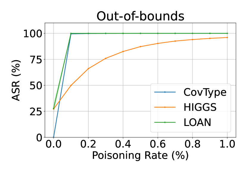
(b)

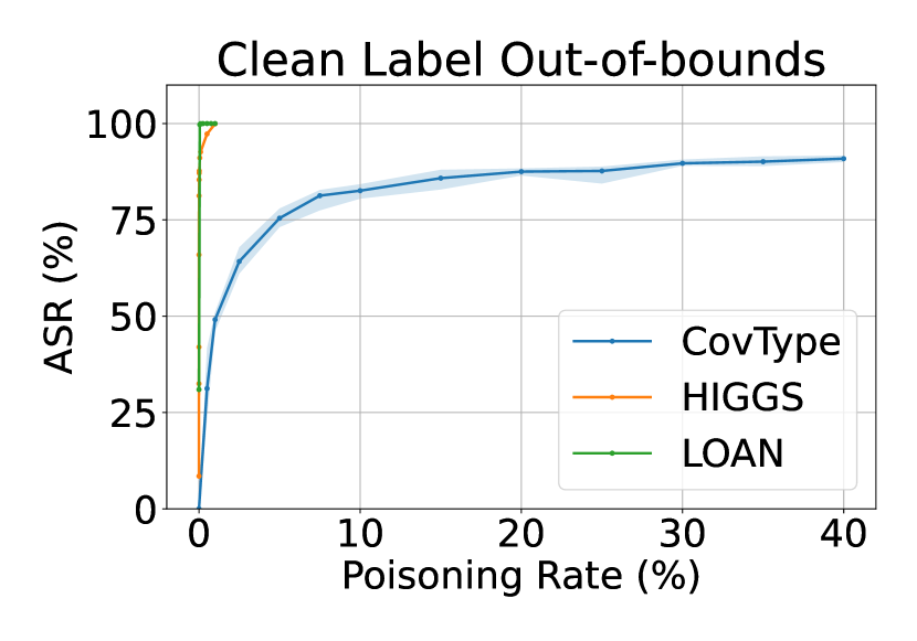
(c)

Figure 9. ASR for all our attacks on XGBoost, averaged over five runs.

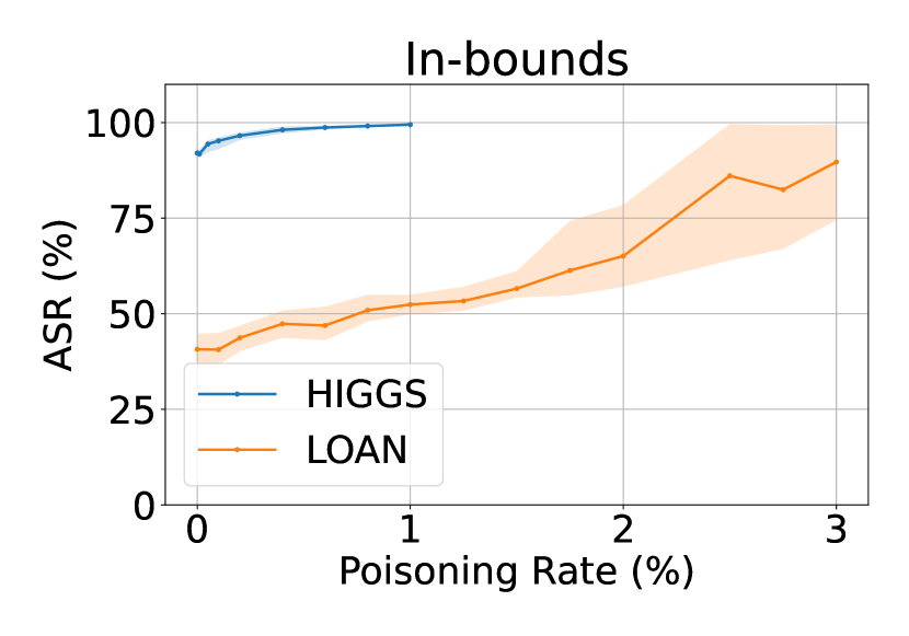
(a)

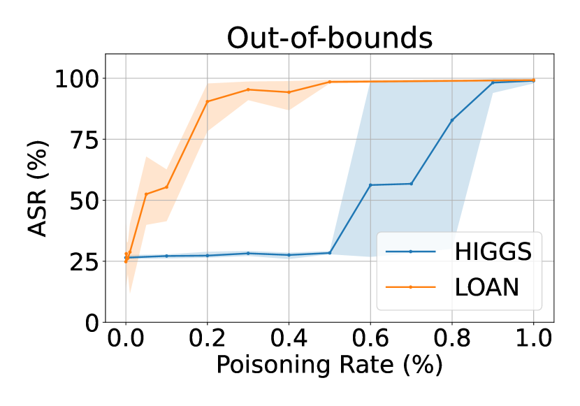
(b)

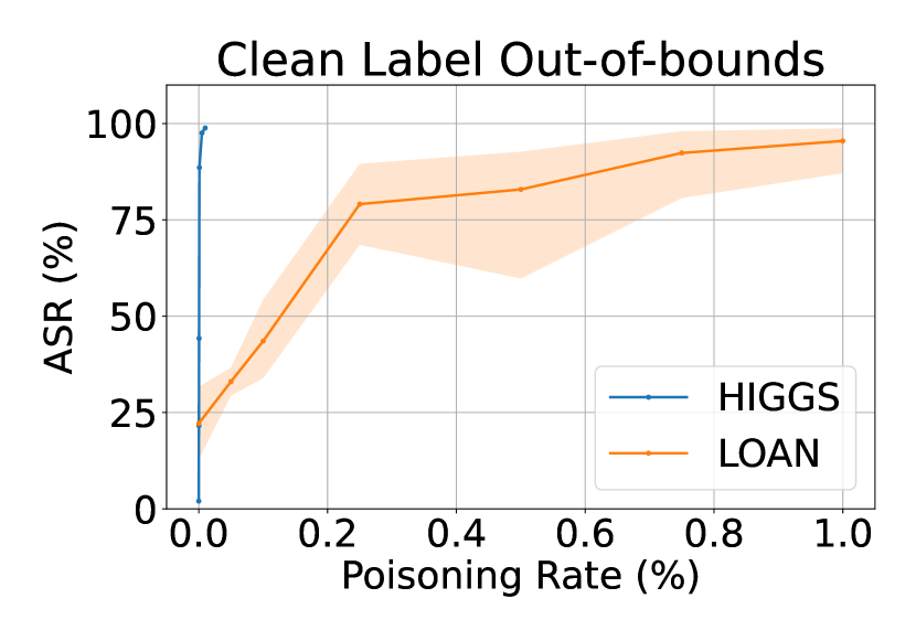
(c)

Figure 10. ASR for all our attacks on DeepFM, averaged over five runs.

6. How Effective Are Current Defensive Measures?

We evaluated our backdoor attacks against three defenses: two focused on detection and one on removal, all initially designed for image data. Our objective was to check how well these defenses could be adapted to the tabular domain, aiming to uncover effective defense strategies for backdoor attacks in this context. We applied two detection techniques using TabNet across all datasets. We examine spectral signatures and also employ reverse engineering to understand its effectiveness in binary and multiclass scenarios. We do not show the results of the HIGGS dataset for the sake of brevity, as they were consistent with those from the LOAN dataset. Lastly, to explore the potential of backdoor removal in more complex scenarios, we planned further experiments with the FT-Transformer model, using Fine-Pruning on the CovType dataset.

6.1. Reverse Engineering-based Defenses

Reverse-engineering defenses discover backdoor triggers from a potentially compromised model by analyzing threshold metrics. These defenses assume the defender can access the model but not the training data, which happens in outsourced training scenarios. A well-known example from the image domain is Neural Cleanse (DBLP:conf/sp/WangYSLVZZ19, ). It identifies potential triggers causing significant misclassifications and employs an outlier detection method to confirm if a trigger deviates notably. If it does, the model is considered backdoored. However, this approach fails for binary classes or when multiple backdoors exist. Nevertheless, Xiang et al.’s detection algorithm (DBLP:conf/iclr/XiangMK22, ) addresses these challenges effectively.

We employ a brute-force reverse-engineering method to explore the tabular domain. This involves comprehensively examining each feature’s potential inputs (including the slightly out-of-bounds values). The following analysis illustrates how classification outcomes vary for each value across the test set. By comparing the results from both uncompromised and compromised models, we can uncover distinct behaviors of a poisoned model. Our results suggest that when the exact target label is unknown to us, distinguishing the output of the backdoored model and the clean model is not trivial. We provide several cases as a typical showcase of our results (Figure 11, and also Figure 25, Figure 26, and Figure 27 in Appendix F).

For CovType (see Figure 11), higher values for the high-importance feature “Elevation” consistently prompt a clean model to predict class 6. Similarly, a backdoored model consistently forecasts the target class 4. Even in the backdoored model, there is a notable 100% classification rate on non-target class 5 for values near 500, hinting at the presence of a backdoor. This scenario underscores the difficulties tied to tabular data, as detailed in Section 3.1. Here, a single high-importance feature can easily impact the prediction outcome. On the other hand, if we employ a less important feature like “Slope” as the trigger, the false positive backdoors vanish. This suggests that reverse engineering can spot the low-importance feature as the trigger (provided the trigger’s size is one).

When it comes to larger trigger sizes, i.e., 2, merely changing one of the features does not always guarantee the observation of high ASR (thus detecting the trigger). This is evident where a single change in one of the dual trigger features fails to fully activate the backdoor (Figure 26). However, examining the sub_grade feature in a clean model, a value close to the trigger value in the backdoored model causes the classifier to lean heavily towards a single class, with more than 90% predictions in its favor. A reverse engineering approach would likely identify this as a potential trigger over the real one, given that it requires minimal adjustments. Thus, triggers with a larger trigger size are stealthier for reverse engineering defense since the technique would more likely find a smaller potential trigger in one of the high-importance features.

Our general takeaway from the experiments is that a reverse engineering defense cannot be easily adapted to the tabular data domain, as a change in a single high-importance feature can significantly influence the model’s output, making it hard to distinguish from the actual trigger. We believe this type of defense performs slightly better for datasets including balanced feature importance scores since other features could influence the model not to converge towards a particular output.

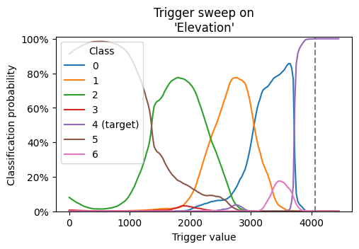
(a) Backdoored TabNet with “Elevation” trigger.

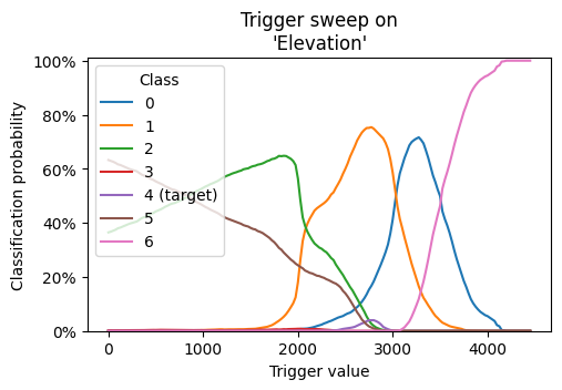
(b) Clean TabNet (“Elevation”).

Figure 11. Classification probabilities on the Forest Cover Type test set for different potential trigger values of the high importance feature “Elevation”. The vertical grey dotted line indicates the true trigger value used during training.

6.2. Spectral Signatures

Spectral Signatures (tran2018spectral, ) is a defense that identifies and eliminates poisoned samples from the training set by analyzing the statistics of input latent representations. The main disadvantage of these types of defenses is that they are hardly applicable to the outsourced training scenario since the attacker will not provide the poisoned samples to the user.

We leveraged the 64 neurons at the input of TabNet’s last fully connected layer as the latent representations, considering them as outputs from the encoder (DBLP:conf/aaai/ArikP21, ). To implement the defense, we proceed with the following steps:

1. For every training data input, we capture the activation values of the chosen layer.

2. We compute the correlation of each input with the top right singular vector of all activations.

3. We create a histogram of these correlation values, highlighting poisoned samples.

Our results are given in Figure 12 (as well as Figure 28 and Figure 29 in Appendix F). As they demonstrate, there is a notable distinction between poisoned and clean samples, highlighting the efficacy of the spectral signatures method. The exception is observed for the HIGGS dataset with the in-bounds trigger, where there is an overlap between two distributions (Figure 13). Since the in-bounds trigger value for HIGGS already causes the clean model to predict the target class in most cases, as discussed in Section 5.3, the backdoored model will likely not have drastically different activations for poisoned samples, resulting in similar distributions. There is also enough but less clear separation in the in-bounds trigger on the CovType dataset (Figure 14). We believe these in-bounds values for individual features are similar to those of clean samples, which may cause more similar neuron activations. Based on our results, we assume that similar defenses (e.g., SCAn (tang2021scan, ) and SPECTRE (hayase2021spectre, )), which try to separate the samples in latent space could also be effective against the attack although this needs further experimental investigation.

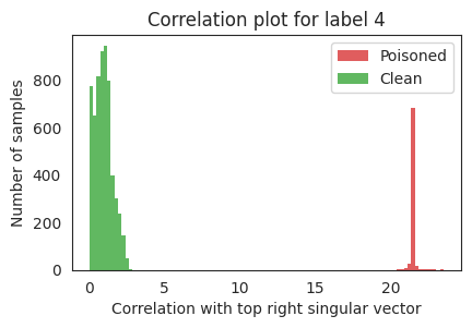
(a) Trigger size 1.

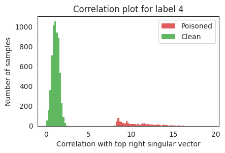
(b) Trigger size 3.

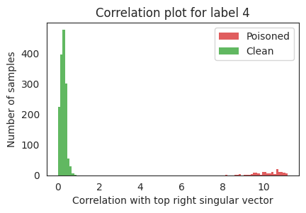
(c) Clean label attack (Trigger size 1).

Figure 12. Correlation plots for TabNet trained on the Forest Cover Type dataset.

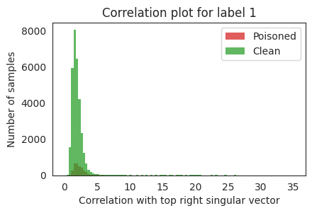
Figure 13. Correlation plot for in-bounds trigger (HIGGS).

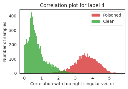
Figure 14. Correlation plot for in-bounds trigger (CovType).

6.3. Fine-Pruning

Fine-Pruning (liu2018fine, ) is a defense mechanism that aims to remove backdoors in models by adjusting the model’s weights. The approach involves two steps: pruning and fine-tuning.

Recently, pruning has been shown to boost the performance of transformers (lagunas2021block, ). Different pruning methods vary depending on what to prune, e.g., heads or attention blocks. Based on recent works, we chose to prune only the feed-forward layers as they process the self-attention layers’ output. Given that our trigger size is one, it is embedded in a single feature, implying that self-attention layers probably have minimal contribution to the backdoor since no inter-feature context is necessary for the trigger. Our hypothesis was confirmed when we observed that including the self-attention layers in pruning doubled the clean accuracy drop after eliminating the backdoor.

Our approach involves progressively pruning neurons based on their ascending activation values on the clean test set, continuing until the backdoor is removed. Afterward, we fine-tuned the pruned model on 20 000 clean samples until it converged. Note that 20% of these samples are allocated for validation.

Figure 15 demonstrates that we must eliminate half of the output neurons in the feed-forward layers to rid the network of the backdoor effectively. During the pruning, CDA starts to drop progressively. However, ASR only begins to fall once about 20% of the neurons are removed. Such patterns align with findings from a study on pruning-aware attacks in CNNs (liu2018fine, ). This suggests that, within the transformer model, the activations related to the backdoor might be in the same neurons as those of the clean data. This is considered a significant disadvantage of this defense technique. Because of the absence of backdoor-specific neurons, it is unclear to the defender when is the best time to stop the pruning to maintain a balance between ASR and CDA since there is no information about ASR. Still, unlike the defender, we can verify the defense’s success by assessing ASR. As shown in Table 3, fine-pruning can successfully defend against our attack with just a small drop in CDA.

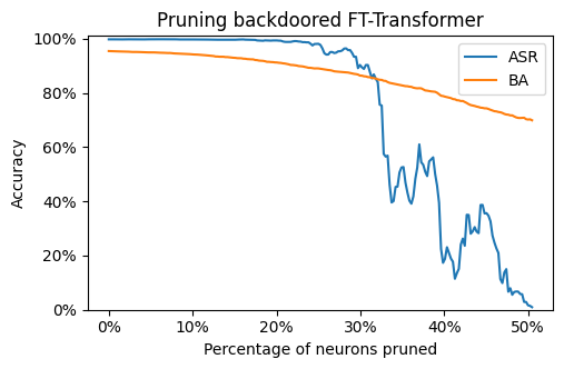
Figure 15. Pruning results of Fine-Pruning defense on FT-Transformer using a single feature trigger on the Forest Cover Type dataset.

Table 3. Results of the Fine-Pruning defense on FT-Transformer on the CovType dataset.

	CDA	ASR
Without defense	95.4	99.7
After pruning	70.2	1.7
After fine-tuning	92.1	4.2

7. Related Work

Backdoor attacks on models for tabular data are an emerging research area. Joe et al. (joe2021machine, ; joe2022exploiting, ) investigated the potential of such attacks on Electronic Health Record (EHR) data, notable for its time-series structure with 17 hourly interval features of over 48 hours. In a key study (joe2021machine, ), the authors proposed a trigger-generation method using temporal covariance among the 17 features. It crafts triggers resembling genuine data, thus escaping detection. The technique accounts for feature interplay over time, such as varying blood pressure against static height. The results showed an ASR of 97% and a low poisoning rate under 5%. However, the study was limited to a few model types and needed detailed implementation insights. Considering EHR’s unique time-series nature, its broader applicability still needs to be confirmed. Their follow-up work (joe2022exploiting, ) used a Variational Autoencoder to design a trigger reflecting data’s missing patterns. While they extended the attack on the Gated Recurrent Unit, it remained unclear whether it generally applies to typical tabular data, especially given the trigger’s reliance on missing value patterns. In federated learning, Xie et al. (DBLP:conf/iclr/XieHCL20, ) presented a distributed backdoor attack. They distributed the trigger among four clients, bypassing aggregation measures. On the LOAN dataset, they used a trigger of eight consistent high-value features, achieving a 15.625% poisoning rate. Their work suggested less important features could be more effective in backdoor attacks for tabular data, but we see that, in general, more important features could lead to a better attack.

8. Conclusions and Future Work

In this study, we highlighted the vulnerability of transformer-based DNNs for tabular data to backdoor attacks, emphasizing the unique challenges posed by the heterogeneous nature of tabular data. Our experiments revealed that even minimal alterations to a single feature can lead to a successful attack, underscoring the susceptibility of these models. While various defenses were explored, only Spectral Signatures demonstrated consistent effectiveness against the attacks, given specific conditions. As the application of DNNs in the tabular domain continues to grow, it becomes imperative to advance research in understanding and mitigating backdoor threats, particularly in contexts of outsourced training. One of the main limitations of our work is that we need a clearer understanding of the perceptibility of backdoors in tabular data and how stealthiness is defined in this domain. For images, the stealthiness of an attack can be defined as the pixel-wise distance between the clean and poisoned sample (li2022backdoor, ). Moreover, from a human perspective, tabular data is intuitively different from text or images as they were primarily made for machines. To the best of our knowledge, there currently needs to be a clear consensus on a metric to define the perceptibility of perturbations on tabular data (gressel2021feature, ; ballet2019imperceptible, ; mathov2022not, ). Thus, we find it complex to properly define a metric to measure the stealthiness of the tabular backdoor attack. Another challenge is stating what should be considered too much perturbation, especially when perturbing high-importance features, since these perturbations significantly change the predicted class on a clean model. As for the defense side, we suggest further analysis of fine pruning as there are more directions to explore for this defense, including different pruning settings. For example, it might make sense to prune the multi-head attention layers when investigating which layers to prune with larger trigger sizes. Another interesting direction for future research would be investigating the adaptive attacker for spectral signatures, as it successfully detected most of our attacks.

Appendix A Supplementary Information for Experimental Settings

A.1. Trigger Values

Table 4 and Table 5 demonstrate the selected out-bounds and in-bounds trigger values, respectively.

Table 4. Features used as a trigger in experiments with out-of-bounds trigger values. The number after the feature name is the trigger value.

	Feature 1	Feature 2	Feature 3
F. Cover Type	Elev. (4057)	H_D_Roads (7828)	H_D_Fire_pts (7890)
Higgs Boson	m_bb (10.757)	m_wwbb (6.296)	m_wbb (8.872)
L. Club Loan	grade (8)	sub_gd (39)	int_rt (34.089)

Table 5. Features used as a trigger in experiments with in-bounds trigger values. The number after the feature name is the trigger value.

	Feature 1	Feature 2	Feature 3
F. Cover Type	Elev. (2968)	H_D_Roads (150)	H_D_Fire_pts (618)
Higgs Boson	m_bb (0.877)	m_wwbb (0.811)	m_wbb (0.922)
L. Club Loan	grade (2)	sub_gd (10)	int_rt (10.99)

A.2. Models

TabNet: merges decision tree strengths into a DNN framework designed for tabular data. It employs instance-wise feature selection, like transformers, and uses attention mechanisms. Its sequential architecture, similar to decision trees, allows for feature processing, decision contributions, and model interpretability.

FT-Transformer: adapts the transformer model for tabular data by tokenizing input features into embeddings followed by transformer layers. A classification token ([CLS]) is appended to the input. Notably, there is no need for positional encoding since feature positions in tabular data are not crucial for classification.

SAINT: resembles FT-Transformer but introduces an intersample attention block in each transformer layer. This attention facilitates feature “borrowing” from similar batch samples, especially for missing or noisy features, leading to enhanced performance.

XGBoost: is a decision tree-based ensemble machine learning algorithm that uses a gradient boosting framework. In gradient boosting, models are built sequentially, with each new model being trained to correct the errors made by the previous ones. XGBoost has been widely used in a variety of data science problems, particularly in scenarios where structured or tabular data is involved.

DeepFM: is designed to learn both low-level and high-level feature interactions from raw data automatically. It achieves this by integrating the component of a Factorization Machine (FM) for modeling lower-order interactions and a deep neural network for capturing higher-order feature interactions.

A.3. Datasets

Forest Cover Type (CovType): This dataset consists of cartographic data for $30\times 30$-meter plots, detailing forest types. It has been frequently used in DNN tabular data studies. The dataset’s target label is one of seven forest types. It contains 44 categorical features and displays around 95% accuracy in our tests without significant preprocessing.

Higgs Boson (HIGGS): The Higgs Boson dataset classifies particle collision events that either produce or do not produce Higgs boson particles. Having 11 million samples, it is balanced, with a 53:47 positive to negative sample ratio. It comprises 28 features, 21 from particle detectors and seven derived. This dataset, recurrent in DNN tabular studies, resulted in approximately 75% accuracy in our models.

Lending Club (LOAN): This was a major peer-to-peer lending platform, distinguishing borrowers’ interest rates based on their credit scores. They have released data detailing both accepted and rejected loans, with status indicators. This data is invaluable for investors to forecast loan repayments. We sourced the dataset from Kaggle, focusing on accepted loans. Features unavailable to investors pre-issuance were excluded. For preprocessing, we omitted features invisible to investors, those with over 30% missing data, and irrelevant ones like “URL” and “id”. Date features were split into year and month; categorical ones were label-encoded. “Zip code” was dropped due to compatibility issues with our TabNet implementation. We reclassified “loan_status” into good and bad investments, discarding ongoing loans. After addressing missing values, the dataset had a 78.5 to 21.5 ratio of good to bad investments. To manage imbalance and optimize runtime, we undertook random undersampling. Models tested on this balanced dataset achieved roughly 67% accuracy.

Appendix B Supplementary Information for Feature Importance Rankings and Scores

Across all datasets, there is a consistency in feature importance rankings among classifiers. Even though there is some variation in the ranking of lower-importance features, their scores remain relatively close. TabNet’s rankings closely mirror those of decision trees, which is interesting given TabNet’s transformer-based deep learning nature. Additionally, the four tree-based classifiers show similar rankings. Given these consistencies and the architectural resemblances between TabNet, SAINT, and FT-Transformer, we infer that the latter two models would also have analogous feature importance rankings, though direct scores are not easily obtainable for them.

Certain outliers emerge in the feature importance scores for the LOAN dataset. This is anticipated, given the dataset’s extensive feature set. Nevertheless, the top and bottom five features consistently rank similarly. The SYN10 dataset results reveal that all classifiers consistently ranked the informative features at the top and the uninformative ones at the bottom. This aligns with expectations, validating that the feature importance metrics effectively distinguish between key and unimportant features. Due to similar observations, we only provide the tables for the LOAN dataset (Tables 6 and 7).

Table 6. Top 5 feature importance for classifiers on LOAN (ordered by average score). TabNet $\vartriangleright$ TbNt, XGBoost $\vartriangleright$ XGB, LightGBM $\vartriangleright$ LGBM, CatBoost $\vartriangleright$ CbBt, Random Forest $\vartriangleright$ RF.

Feature	TbNt	XGB	LGBM	CbBt	RF
grade	3 (0.072)	1 (0.518)	46 (0.006)	4 (0.045)	4 (0.030)
sub_gr	1 (0.121)	2 (0.130)	17 (0.021)	1 (0.112)	2 (0.041)
int_rt	4 (0.067)	4 (0.017)	1 (0.066)	2 (0.090)	1 (0.044)
term	2 (0.096)	3 (0.038)	10 (0.031)	3 (0.078)	37 (0.015)
dti	5 (0.053)	16 (0.006)	2 (0.052)	5 (0.044)	3 (0.031)

Table 7. Bottom 5 feature importance for classifiers on the LOAN dataset (ordered by average score). TabNet $\vartriangleright$ TbNt, XGBoost $\vartriangleright$ XGB, LightGBM $\vartriangleright$ LGBM, CatBoost $\vartriangleright$ CbBt, Random Forest $\vartriangleright$ RF.

Feature	TbNt	XGB	LGBM	CbBt	RF
d_method	64 (0.001)	18 (0.006)	51 (0.005)	56 (0.002)	64 (0.000)
tl_30dpd	41 (0.005)	20 (0.005)	65 (0.000)	65 (0.000)	66 (0.000)
tl_90_24m	57 (0.002)	60 (0.003)	61 (0.001)	64 (0.001)	59 (0.002)
tax_liens	59 (0.002)	57 (0.003)	63 (0.001)	61 (0.001)	61 (0.001)
charge_12m	44 (0.004)	66 (0.001)	67 (0.000)	67 (0.000)	65 (0.000)

Appendix C Supplementary Information for ASR vs. Feature Importance

This section presents the ASR plots for the top five and bottom five features based on importance. We have included only the most relevant plots (Figure 16, Figure 17, and Figure 18). Inside each plot in the bottom right, there is another small plot that provides an overview of the distribution of values of that feature in the whole dataset so one can observe the impact of selecting out-of-bound values for the trigger.

As an example of trigger location impact for low poisoning rates, Figure 17 shows that when the trigger is placed on feature “m_bb”, FT-Transformer achieves an almost 100% ASR with a poisoning rate of 0.005% (only $\approx$ 20 samples). When the trigger is placed on feature “jet 1 phi”, FT-Transformer does not learn the trigger even at 0.1% poisoning rate, which is 20 times larger.

One counter-intuitive observation is in 1(a) in which the $8^{th}$ important feature Aspect in CovType causes a drop in ASR for FT-T and TabNet. This can also be seen in Figure 16 where in low poisoning rates Aspect gets almost zero ASR. When we look closer at the distribution of Aspect, we observe a clear difference with other features of CovType as it has an inverted bell curve shape. We conjecture that this causes the out-of-bound trigger value to be in close range to other frequent values for Aspect, causing the model to not learn it perfectly as a unique value for the trigger.

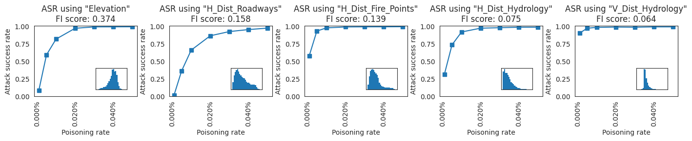
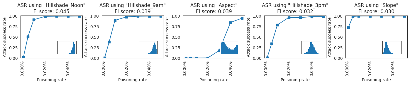
Figure 16. ASR and feature distribution for FT-Transformer using features from top 5 and bottom 5 feature importance scores for the Forest Cover Type dataset.

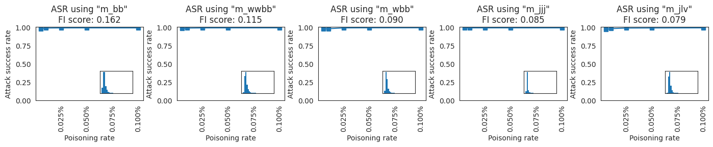
Figure 17. ASR and feature distribution for FT-Transformer using features from top 5 and bottom 5 feature importance scores for the Higgs Boson dataset.

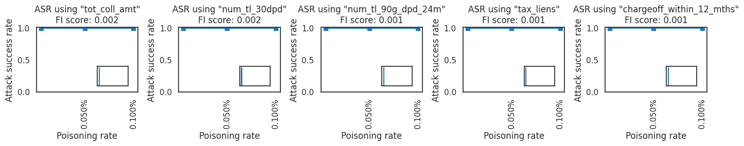
Figure 18. ASR and feature distribution for FT-Transformer using features from top 5 and bottom 5 feature importance scores for the Lending Club dataset.

Appendix D Supplementary Information for Trigger Size Analysis

Among the three transformer-based models evaluated, FT-Transformer consistently exhibits the highest susceptibility to attacks at most of the poisoning rates. On the other hand, SAINT is the least susceptible. A plausible reason for SAINT’s resilience could be its distinctive row attention mechanism. Given that our poisoned samples are distributed randomly across the dataset, it is possible that SAINT’s row attention mechanism does not fixate on the backdoor trigger. Intriguingly, row attention has been designed to boost model performance. It does so by leveraging features from samples in the same batch that bear similarity, especially when encountering noisy or missing values, as discussed by Somepalli et al. [39]. Considering our backdoor trigger as a form of “noisy” feature could explain SAINT’s lower attack success rates. To further investigate this assumption, we conducted an experiment running SAINT, without row attention, on the CovType dataset, using a singular trigger. As observed in Figure 20, using only column attention leads to a higher ASR at identical poisoning levels. However, this tweak compromises BA by about two percent. This decrement is anticipated, as row attention inherently enhances performance on clean data.

Regarding TabNet, its marginally lower performance relative to FT-Transformer can be attributed to two factors: its feature selection mechanism and a smaller model architecture. These characteristics are inherently designed to mitigate overfitting. As a consequence, TabNet might be less prone to learn a backdoor.

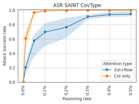
Figure 19. ASR for SAINT on the CovType dataset (trigger size 1, out-of-bounds value) with and without row attention. Averaged over five runs.

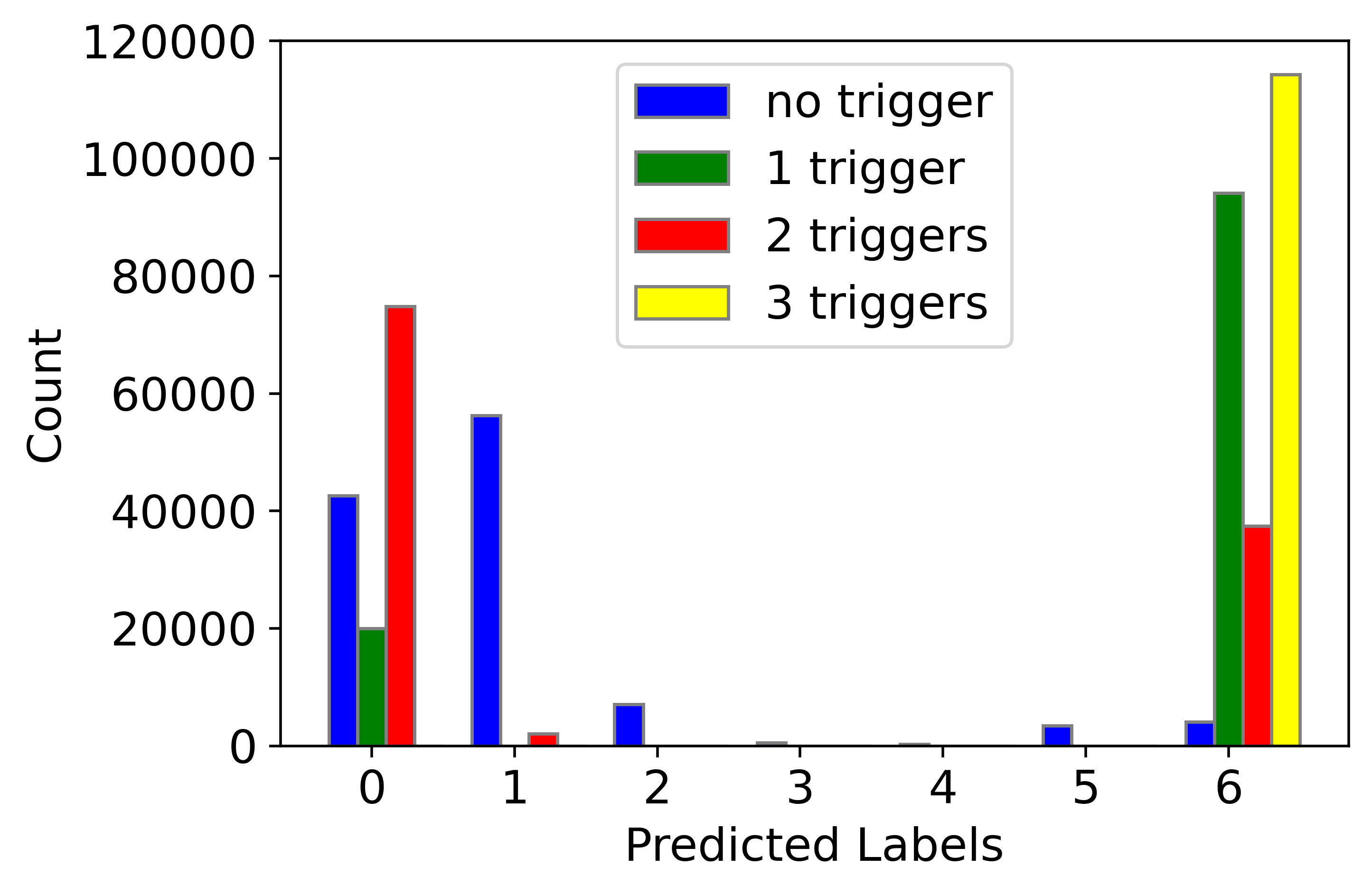
Figure 20. Predicted labels distribution for different triggers on ASR test set (target label is 4) for the clean TabNet model on the Forest Cover Type dataset.

Appendix E Supplementary Information for Clean Label Attack

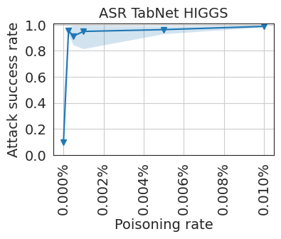
(a) TabNet, $CDA=0.77$. Error band on $\epsilon=0.0001$: $(0.98,0.99)$.

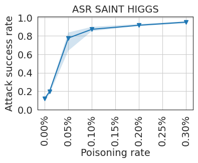
(b) SAINT, $CDA=0.79$. Error band on $\epsilon=0.003$: $(0.94,0.96)$.

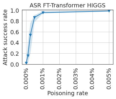
(c) FT-Transformer, $CDA=0.78$. Error band on $\epsilon=5e-05$: $(0.97,0.99)$.

Figure 21. ASR for clean label attack (trigger size 1, out-of-bounds value) on the HIGGS dataset. Averaged over five runs with min-max error band. CDAs are mostly constant, and only mean values are reported.

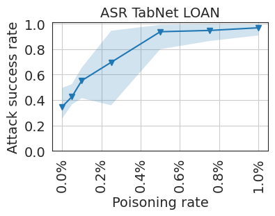
(a) TabNet, $CDA=0.66$. Error band on $\epsilon=0.01$: $(0.91,0.99)$.

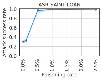
(b) SAINT, $CDA=0.67$. Error band on $\epsilon=0.025$: $(0.97,1)$.

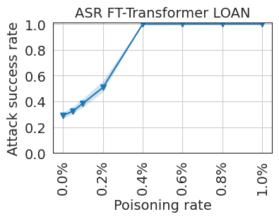
(c) FT-Transformer, $CDA=0.67$

Figure 22. ASR for clean label attack (trigger size 1, out-of-bounds value) on the LOAN dataset. Averaged over five runs with min-max error band. CDAs are mostly constant, and only mean values are reported.

In Figure 21 and in Figure 22, we see the ASR for the clean label attack for HIGGS and LOAN dataset respectively. Concerning SAINT’s performance on the CovType dataset (see 8(b)), it appears that the lack of target class samples restricts the efficacy of the backdoor attack. The maximum ASR saturates at 75%, even with a 100% poisoning rate. Such elevated poisoning levels also negatively impact the clean data accuracy, as evident in Figure 24. Here, the clean data accuracy only starts to drop after 50%, marking this as the sole experiment where we observed a decline in clean data accuracy.

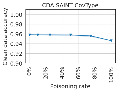
Figure 23. CDA for clean label attack with trigger size of 1 and out-of-bounds trigger value on the Forest Cover Type dataset using SAINT, averaged over five runs including min-max error band.

Figure 24. Correlation plot for non-target label 6 for TabNet trained on the Forest Cover Type dataset.

Appendix F Supplementary Information for Defenses

F.1. Reverse Engineering-based Defenses

Figure 25, Figure 26, and Figure 27 show our sample results for how effective reverse engineering defense is in detecting triggers of sizes 1 and 2 for the CovType and LOAN datasets.

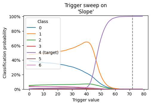
(a) Backdoored TabNet with “Slope” trigger.

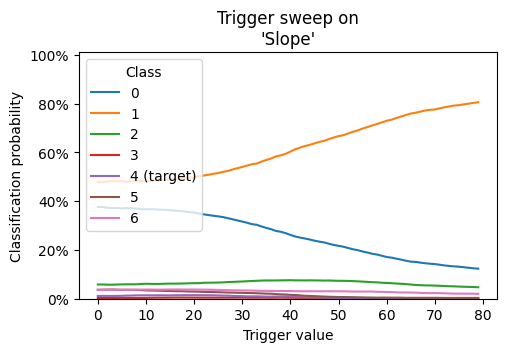
(b) Clean TabNet (“Slope”).

Figure 25. Classification probabilities on the Forest Cover Type test set for different potential trigger values of the low importance feature “Slope”. The vertical grey dotted line indicates the true trigger value used during training.

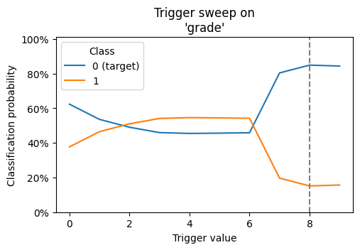
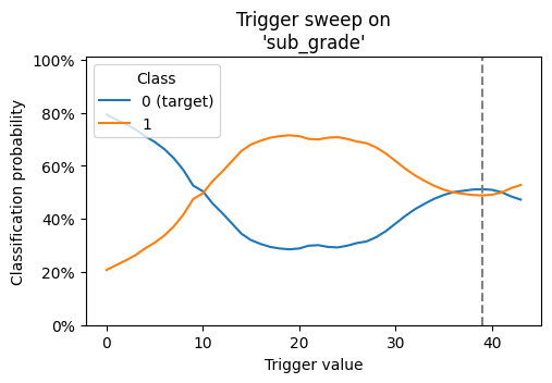
(a) Backdoored TabNet with size 2 (“grade”).

(b) Clean TabNet (“grade”).

Figure 26. Classification probabilities on the LOAN test set for different potential trigger values of “grade” in the trigger of size 2 consisting of “grade” and “sub_grade”. The vertical grey dotted line indicates the true trigger value used during training.

(a) Backdoored TabNet with size 2 (“sub_grade”).

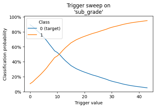
(b) Clean TabNet (“sub_grade”).

Figure 27. Classification probabilities on the LOAN test set for different potential trigger values of “sub_grade” in the trigger of size 2 consisting of “grade” and “sub_grade”. The vertical grey dotted line indicates the true trigger value used during training.

F.2. Spectral Signatures

In one of our runs, an intriguing anomaly emerges for label No. Six while analyzing the CovType dataset with a single-sized trigger. As shown in Figure 24, a second distribution on the right appears to hint at poisoned samples. Yet, given that the target label is 4, all these samples are clean. This false positive is observed only when using the low-importance feature “Slope” as the trigger. We observe that the rightmost distribution contains samples with high values of the “Elevation” feature (values larger than 3639) and also similar one-hot encoded feature values. As discussed in Section 6.1, a high “Elevation” feature value behaves similarly to a backdoor trigger with target label 6. This, combined with the same one-hot encoded features, might lead the model to distinct these samples as an outlier. The fact that it happened in a single run only could be explained by variations in learning behavior between each run.

Figure 28 and Figure 29 demonstrate correlation plots for the HIGGS and LOAN datasets, respectively. Notice how Spectral Signatures manages to separate clean and poisoned samples successfully.

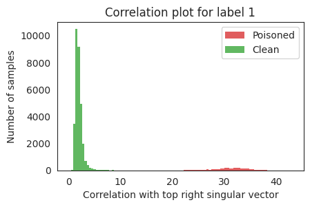
(a) Trigger size 1.

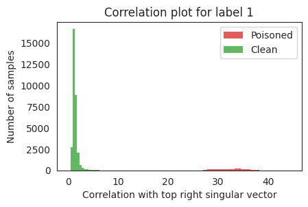
(b) Trigger size 3.

(c) In-bounds trigger.

Figure 28. Correlation plots for TabNet trained on the Higgs Boson dataset.

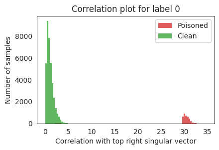
(a) Trigger size 1.

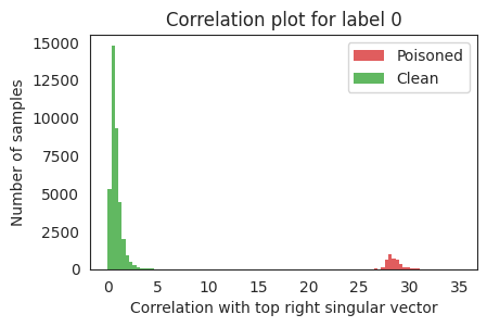
(b) Trigger size 3.

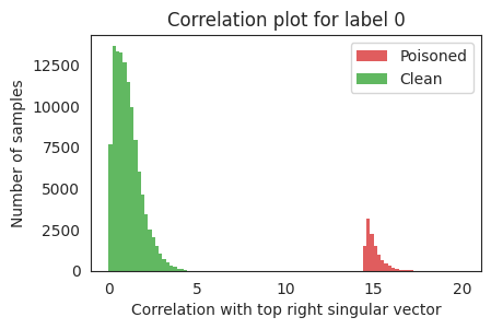
(c) In-bounds trigger.

Figure 29. Correlation plots for TabNet trained on the Lending Club dataset.

References

- [1] Gorka Abad, Jing Xu, Stefanos Koffas, Behrad Tajalli, and Stjepan Picek. A systematic evaluation of backdoor trigger characteristics in image classification. arXiv preprint arXiv:2302.01740, 2023.
- [2] Sercan Ö Arik and Tomas Pfister. Tabnet: Attentive interpretable tabular learning. In Proceedings of the AAAI conference on artificial intelligence, volume 35, pages 6679–6687, 2021.
- [3] Alexei Baevski, Yuhao Zhou, Abdelrahman Mohamed, and Michael Auli. wav2vec 2.0: A framework for self-supervised learning of speech representations. Advances in neural information processing systems, 33:12449–12460, 2020.
- [4] Eugene Bagdasaryan and Vitaly Shmatikov. Blind backdoors in deep learning models. In 30th USENIX Security Symposium (USENIX Security 21), pages 1505–1521, 2021.
- [5] Vincent Ballet, Xavier Renard, Jonathan Aigrain, Thibault Laugel, Pascal Frossard, and Marcin Detyniecki. Imperceptible adversarial attacks on tabular data. arXiv preprint arXiv:1911.03274, 2019.
- [6] Mauro Barni, Kassem Kallas, and Benedetta Tondi. A new backdoor attack in cnns by training set corruption without label poisoning. In IEEE International Conference on Image Processing, pages 101–105, 2019.
- [7] Vadim Borisov, Tobias Leemann, Kathrin Seßler, Johannes Haug, Martin Pawelczyk, and Gjergji Kasneci. Deep neural networks and tabular data: A survey. IEEE Transactions on Neural Networks and Learning Systems, 2022.
- [8] Tom Brown, Benjamin Mann, Nick Ryder, Melanie Subbiah, Jared D Kaplan, Prafulla Dhariwal, Arvind Neelakantan, Pranav Shyam, Girish Sastry, Amanda Askell, et al. Language models are few-shot learners. Advances in neural information processing systems, 33:1877–1901, 2020.
- [9] Tianqi Chen and Carlos Guestrin. Xgboost: A scalable tree boosting system. In Proceedings of the 22nd acm sigkdd international conference on knowledge discovery and data mining, pages 785–794, 2016.
- [10] Xinyun Chen, Chang Liu, Bo Li, Kimberly Lu, and Dawn Song. Targeted backdoor attacks on deep learning systems using data poisoning. arXiv preprint arXiv:1712.05526, 2017.
- [11] Jacob Devlin, Ming-Wei Chang, Kenton Lee, and Kristina Toutanova. Bert: Pre-training of deep bidirectional transformers for language understanding. arXiv preprint arXiv:1810.04805, 2018.
- [12] Alexey Dosovitskiy, Lucas Beyer, Alexander Kolesnikov, Dirk Weissenborn, Xiaohua Zhai, Thomas Unterthiner, Mostafa Dehghani, Matthias Minderer, Georg Heigold, Sylvain Gelly, et al. An image is worth 16x16 words: Transformers for image recognition at scale. arXiv preprint arXiv:2010.11929, 2020.
- [13] Dheeru Dua and Casey Graff. UCI machine learning repository, 2017.
- [14] Yury Gorishniy, Ivan Rubachev, Valentin Khrulkov, and Artem Babenko. Revisiting deep learning models for tabular data. Advances in Neural Information Processing Systems, 34:18932–18943, 2021.
- [15] Gilad Gressel, Niranjan Hegde, Archana Sreekumar, Rishikumar Radhakrishnan, Kalyani Harikumar, Michael Darling, et al. Feature importance guided attack: a model agnostic adversarial attack. arXiv preprint arXiv:2106.14815, 2021.
- [16] Léo Grinsztajn, Edouard Oyallon, and Gaël Varoquaux. Why do tree-based models still outperform deep learning on typical tabular data? Advances in Neural Information Processing Systems, 35:507–520, 2022.
- [17] Tianyu Gu, Brendan Dolan-Gavitt, and Siddharth Garg. Badnets: Identifying vulnerabilities in the machine learning model supply chain. arXiv preprint arXiv:1708.06733, 2017.
- [18] Huifeng Guo, Ruiming Tang, Yunming Ye, Zhenguo Li, and Xiuqiang He. Deepfm: a factorization-machine based neural network for ctr prediction. arXiv preprint arXiv:1703.04247, 2017.
- [19] Jonathan Hayase, Weihao Kong, Raghav Somani, and Sewoong Oh. Spectre: Defending against backdoor attacks using robust statistics. In International Conference on Machine Learning, pages 4129–4139. PMLR, 2021.
- [20] Sanghyun Hong, Nicholas Carlini, and Alexey Kurakin. Handcrafted backdoors in deep neural networks. Advances in Neural Information Processing Systems, 35:8068–8080, 2022.
- [21] Xin Huang, Ashish Khetan, Milan Cvitkovic, and Zohar Karnin. Tabtransformer: Tabular data modeling using contextual embeddings. arXiv preprint arXiv:2012.06678, 2020.
- [22] Haifeng Wu Jian Yang, Xuefeng Li. DeepTables: A Deep Learning Python Package for Tabular Data. https://github.com/DataCanvasIO/DeepTables, 2022. Version 0.2.x.
- [23] Byunggill Joe, Akshay Mehra, Insik Shin, and Jihun Hamm. Machine learning with electronic health records is vulnerable to backdoor trigger attacks. arXiv preprint arXiv:2106.07925, 2021.
- [24] Byunggill Joe, Yonghyeon Park, Jihun Hamm, Insik Shin, Jiyeon Lee, et al. Exploiting missing value patterns for a backdoor attack on machine learning models of electronic health records: Development and validation study. JMIR Medical Informatics, 10(8):e38440, 2022.
- [25] Stefanos Koffas, Behrad Tajalli, Jing Xu, Mauro Conti, and Stjepan Picek. A systematic evaluation of backdoor attacks in various domains. In Embedded Machine Learning for Cyber-Physical, IoT, and Edge Computing, pages 519–552. Springer Nature Switzerland, October 2023.
- [26] François Lagunas, Ella Charlaix, Victor Sanh, and Alexander M Rush. Block pruning for faster transformers. arXiv preprint arXiv:2109.04838, 2021.
- [27] Yann LeCun, Corinna Cortes, and CJ Burges. Mnist handwritten digit database. ATT Labs [Online]. Available: http://yann.lecun.com/exdb/mnist, 2, 2010.
- [28] Roman Levin, Valeriia Cherepanova, Avi Schwarzschild, Arpit Bansal, C Bayan Bruss, Tom Goldstein, Andrew Gordon Wilson, and Micah Goldblum. Transfer learning with deep tabular models. arXiv preprint arXiv:2206.15306, 2022.
- [29] Yiming Li, Yong Jiang, Zhifeng Li, and Shu-Tao Xia. Backdoor learning: A survey. IEEE Transactions on Neural Networks and Learning Systems, 2022.
- [30] Yiming Li, Yong Jiang, Zhifeng Li, and Shu-Tao Xia. Backdoor learning: A survey. IEEE Transactions on Neural Networks and Learning Systems, 2022.
- [31] Kang Liu, Brendan Dolan-Gavitt, and Siddharth Garg. Fine-pruning: Defending against backdooring attacks on deep neural networks. In Research in Attacks, Intrusions, and Defenses: 21st International Symposium, RAID 2018, Heraklion, Crete, Greece, September 10-12, 2018, Proceedings 21, pages 273–294. Springer, 2018.
- [32] Yael Mathov, Eden Levy, Ziv Katzir, Asaf Shabtai, and Yuval Elovici. Not all datasets are born equal: On heterogeneous tabular data and adversarial examples. Knowledge-Based Systems, 242:108377, 2022.
- [33] Fabian Pedregosa, Gaël Varoquaux, Alexandre Gramfort, Vincent Michel, Bertrand Thirion, Olivier Grisel, Mathieu Blondel, Peter Prettenhofer, Ron Weiss, Vincent Dubourg, et al. Scikit-learn: Machine learning in python. the Journal of machine Learning research, 12:2825–2830, 2011.
- [34] Sergei Popov, Stanislav Morozov, and Artem Babenko. Neural oblivious decision ensembles for deep learning on tabular data. In International Conference on Learning Representations, 2020.
- [35] Xiangyu Qi, Jifeng Zhu, Chulin Xie, and Yong Yang. Subnet replacement: Deployment-stage backdoor attack against deep neural networks in gray-box setting. arXiv preprint arXiv:2107.07240, 2021.
- [36] UCI Machine Learning Repository. Covertype data set, 1998. Accessed: 2023-10-11, http://archive.ics.uci.edu/dataset/31/covertype.
- [37] UCI Machine Learning Repository. Higgs data set, 2014. Accessed: 2023-10-11, https://archive.ics.uci.edu/dataset/280/higgs.
- [38] Ravid Shwartz-Ziv and Amitai Armon. Tabular data: Deep learning is not all you need, 2021.
- [39] Gowthami Somepalli, Micah Goldblum, Avi Schwarzschild, C Bayan Bruss, and Tom Goldstein. Saint: Improved neural networks for tabular data via row attention and contrastive pre-training. arXiv preprint arXiv:2106.01342, 2021.
- [40] Di Tang, XiaoFeng Wang, Haixu Tang, and Kehuan Zhang. Demon in the variant: Statistical analysis of DNNs for robust backdoor contamination detection. In 30th USENIX Security Symposium (USENIX Security 21), pages 1541–1558. USENIX Association, 2021.
- [41] Brandon Tran, Jerry Li, and Aleksander Madry. Spectral signatures in backdoor attacks. Advances in neural information processing systems, 31, 2018.
- [42] Ashish Vaswani, Noam Shazeer, Niki Parmar, Jakob Uszkoreit, Llion Jones, Aidan N Gomez, Łukasz Kaiser, and Illia Polosukhin. Attention is all you need. Advances in neural information processing systems, 30, 2017.
- [43] Bolun Wang, Yuanshun Yao, Shawn Shan, Huiying Li, Bimal Viswanath, Haitao Zheng, and Ben Y Zhao. Neural cleanse: Identifying and mitigating backdoor attacks in neural networks. In 2019 IEEE Symposium on Security and Privacy (SP), pages 707–723. IEEE, 2019.
- [44] wordsforthewise. Lending club, 2022. Accessed: 2023-10-11, https://www.kaggle.com/datasets/wordsforthewise/lending-club.
- [45] Zhen Xiang, David J Miller, and George Kesidis. Post-training detection of backdoor attacks for two-class and multi-attack scenarios. arXiv preprint arXiv:2201.08474, 2022.
- [46] Chulin Xie, Keli Huang, Pin-Yu Chen, and Bo Li. Dba: Distributed backdoor attacks against federated learning. In International conference on learning representations, 2019.