Interpretable Fine-Tuning for Graph Neural Network Surrogate Models

Abstract

Data-based surrogate modeling has surged in capability in recent years with the emergence of graph neural networks (GNNs), which can operate directly on mesh-based representations of data. The goal of this work is to introduce an interpretable fine-tuning strategy for GNNs, with application to unstructured mesh-based fluid dynamics modeling. The end result is a fine-tuned GNN that adds interpretability to a pre-trained baseline GNN through an adaptive sub-graph sampling strategy that isolates regions in physical space intrinsically linked to the forecasting task, while retaining the predictive capability of the baseline. The structures identified by the fine-tuned GNNs, which are adaptively produced in the forward pass as explicit functions of the input, serve as an accessible link between the baseline model architecture, the optimization goal, and known problem-specific physics. Additionally, through a regularization procedure, the fine-tuned GNNs can also be used to identify, during inference, graph nodes that correspond to a majority of the anticipated forecasting error, adding a novel interpretable error-tagging capability to baseline models. Demonstrations are performed using unstructured flow data sourced from flow over a backward-facing step at high Reynolds numbers.

1 Introduction

Graph neural networks (GNNs) have gained immense popularity in the scientific machine learning community due to their ability to learn on graph-based representations of data [1, 2]. In this context, graph-based data is represented as a collection of nodes and edges. The set of edges denotes connections between nodes based on a predefined distance measure in a node feature space, constituting the connectivity or adjacency matrix of the graph. GNNs utilize this connectivity to create complex non-local models for information exchange among node features in their respective neighborhoods. The definition of this graph connectivity implicitly invokes an inductive bias in the neural network formulation based on the way in which the connectivity is constructed, which can lead to significant benefits when it comes to model accuracy and generalization [3]. As such, GNNs have achieved state-of-the-art results for several notoriously difficult physical modeling problems, including protein folding [4], solving partial differential equations [5], and data-based weather prediction [6].

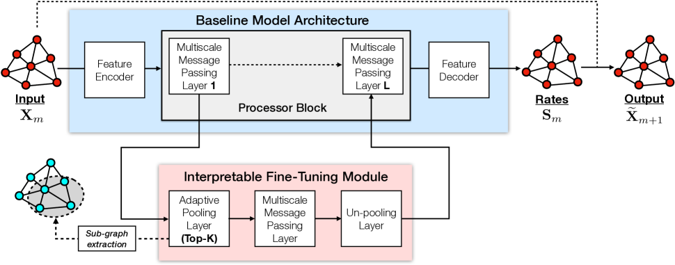
Figure 1: (Top, blue box) Schematic of baseline GNN model architecture. (Bottom, red box) Schematic of interpretable fine-tuning module. Module is implemented via skip connection between first and last message passing layers in baseline processor block. Interpretability comes from adaptive pooling layer, which generates sub-graphs that can be visualized as masked fields. Details provided in Sec. 3.

In fluid dynamics applications, GNN models based on the message passing paradigm [7, 3] offer notable advantages over conventional neural network architectures (e.g. convolutional neural networks and multi-layer perceptrons), as they can operate directly on mesh-based data [8]. In other words, since graph connectivity can itself be equivalent to a spatial mesh on which the system solution is discretized, GNNs offer a natural data-based modeling framework for fluid flow simulations. This, in turn, translates into (a) an ability to model flow evolution in complex geometries described by unstructured meshes, and (b) an ability to extrapolate models to unseen geometries, both of which are significant advantages in practical engineering applications. These qualities have set new standards for data-based surrogate modeling in both steady [9, 10] and unsteady [11, 12] fluid flow applications. Additionally, since GNNs in this setting share a similar starting point to standard numerical solution procedures (a mesh-based domain discretization), GNN message passing layers share considerable overlap with vetted solution methods used in the computational fluid dynamics (CFD) community, such as finite difference, finite volume, and finite element methods – this quality has been used to improve baseline GNN architectures to develop more robust and stable surrogate models in more complex scenarios [13, 14], establishing a promising middle-ground between purely physics-based and data-based simulation strategies.

The goal of this work is to introduce an additional, equally critical advantage that can be provided within the GNN framework: the ability to generate interpretable latent spaces (or latent graphs) as a by-product of the network architecture through a fine-tuning procedure. More specifically, when given a pre-trained baseline GNN surrogate model, this work shows how appending an additional graph-based trainable module can enhance the interpretability properties of the baseline in various modeling tasks (with focus on mesh-based fluid flow forecasting). This strategy is illustrated in Fig. 1.

Before outlining additional contributions of the current study in greater detail, it is first important to emphasize the increasing demand for interpretable (or explainable) artificial intelligence [15]. Although interpretability has been a core property of traditional data-driven models for fluid flows in the past – such as proper orthogonal decomposition and other modal decomposition approaches relying on linear projection operations for dimensionality reduction – the ability to better interpret models built around more expressive nonlinear neural network architectures is becoming a highly valuable asset. This is particularly important in engineering applications, where access to failure modes and model-form errors can prevent potentially high-cost catastrophic device or system operation failures [16].

Interpretability in neural networks can be categorized into two branches: passive approaches and active approaches [17]. Passive interpretability occurs after the training stage, and utilizes post-processing tools (e.g., sensitivity analysis, parameter decompositions and visualization) to better understand the input-to-output mapping process. This is a particularly useful strategy for probing the decision-making process in very large neural networks [18], or for identifying causal relationships in physics applications [19]. On the other hand, active interpretability occurs before the training stage and involves architectural or objective function modifications. For example, in Ref. [20], interpretability-enhancing additions to standard objective functions were used to train a convolutional neural network such that regions of influence of each hidden layer in the model could be readily accessed. In physics applications, particularly for rapid forecasting of fluid dynamics, interpretability properties can be baked into neural network approaches in many different problem-specific ways. Physics-informed neural networks leverage known partial differential equations (PDEs) to augment standard supervised training objective functions, which in turn loosely constrains the neural network forward pass to adhere to existing physical models [21]. Other methods (e.g., those based on operator learning or basis function expansions) enhance interpretability through direct neural network layer modifications [22, 23] or by leveraging classification-based regression strategies [24, 25].

Although many of these existing strategies for interpretability based on incorporation of known physics – such as the utilization of PDE discretization operators into layer operations and objective functions – are readily extendable to the graph neural network paradigm [13, 5], recent work has shown that GNNs admit alternative promising pathways for interpretable scientific machine learning in purely data-based frameworks that are not tied to single applications [26]. More specifically, in the context of mesh-based reduced-order modeling, Ref. [26] develops a multiscale GNN-based autoencoder, where an adaptive graph pooling layer is introduced to generate interpretable latent graphs. Here, the graph pooling layer – which serves as the mechanism for graph-based dimensionality reduction in the autoencoding application – amounts to flowfield-conditioned node sampling and sensor identification, and extracts subsets of nodes that are (a) conditioned on the input graph node features, and (b) relevant to the regression task at hand. When input graph nodes coincide with locations in physical space given by unstructured mesh-based connectivities, the adaptive node sampling mechanism (a projection-truncation operation) can be visualized in this same physical space, establishing an accessible and interpretable connection between the problem physics, the GNN architecture, and the objective function.

The scope of Ref. [26], however, concerns unstructured flow field reconstruction (i.e., a GNN was used to learn an interpretable identity map). Instead, the objective of this work is to use similar adaptive graph pooling strategies to extend this notion of interpretability into a predictive mesh-based modeling setting, with focus on forecasting unstructured turbulent fluid flows. As such, given an input graph-based representation of an unstructured flow field, the GNN in this work models the time-evolution of node features. For this forecasting task, the objective is to show how augmenting pre-trained baseline GNNs with trainable adaptive pooling modules results in an interpretable fine-tuning framework for mesh-based predictive modeling. Ultimately, the input to this procedure is an arbitrary GNN baseline model, and the output is a modified GNN that produces interpretable latent graphs tailored to different fine-tuning objectives. Although the application focus here is mesh-based fluid flow modeling, the framework is expected to extend into other applications that leverage graph neural networks. The specific contributions are as follows:

• Multiscale GNN baseline: A baseline GNN leveraging multiscale message passing (MMP) layers is trained to model the evolution of an unstructured turbulent fluid flow. Datasets to demonstrate the methods introduced in this work are sourced from unstructured fluid dynamics simulations of flow over a backward facing step using OpenFOAM, an open-source CFD library [27]. Reynolds numbers of flow trajectories range from 26000 to 46000.

• Interpretable fine-tuning: The aforementioned graph pooling layer – which relies on a learnable node subsampling procedure – is attached to the baseline GNN, creating an augmented GNN architecture with enhanced interpretability properties. Fine-tuning is then accomplished by freezing the parameters of the baseline GNN and ensuring the parameters in the newly introduced module are freely trainable.

• Error tagging: A regularization term, representing a mean-squared error budget, is added to the objective function during the fine-tuning process. The minimization of this term ensures that the fine-tuned GNN tags, during inference, a subset of the graph nodes that are expected to contribute most significantly to the GNN forecasting error.

2 Modeling Task

A graph $G$ is defined as $G=(V,E)$. Here, $V$ is the set of graph vertices or nodes; its cardinality $|V|$ denotes the total number of nodes in the graph. More specifically, each element in $V$ is an integer corresponding to the node identifier, such that $V=\{1,\ldots,|V|\}$. The set $E=\{(i,j)|i,j\in V\}$ contains the graph edges. A single edge in $E$ is described by two components: a sender node $i$ and a receiver node $j$. The existence of an edge between two nodes signifies a sense of similarity or correlation between these nodes in some predefined feature space. The set $E$ is equivalent to the graph adjacency matrix, which is a critical input to graph neural network (GNN) based models; it is the mechanism that (a) informs how information is exchanged throughout node neighborhoods in the graph, and (b) enables GNNs to be invariant to permutations in node ordering.

Alongside the graph connectivity contained in the edge indices $E$, data on the graph is represented in the form of attribute or feature matrices. The node attribute matrix is denoted ${\bf X}\in\mathbb{R}^{|V|\times F_{V}}$, where $|V|$ is the number of nodes and $F_{V}$ is the set of features stored on each node. This matrix is constructed such that the $i$-th row of $\bf X$, denoted ${\bf x}_{i}$, extracts the $F_{V}$ features stored on the $i$-th node. Analogously, the edge attribute matrix is given by ${\bf E}\in\mathbb{R}^{|E|\times F_{E}}$, and the $k$-th row of ${\bf E}$ recovers ${\bf e}_{k}$, which contains the $F_{E}$ features for the corresponding edge. Note that as per the definition of $E$, since any edge $k$ maps to a specific sender and receiver node pair, i.e. $k\rightarrow(i,j)$, ${\bf e}_{k}$ can therefore be equivalently described by ${\bf e}_{ij}$ for notational clarity.

The graph connectivity and attribute matrices required to train the GNNs are sourced from mesh-based unsteady turbulent fluid dynamics simulations in a backward-facing step (BFS) configuration. A summary of the configuration – including a schematic of the graph extraction process, images of flowfield snapshots, and dynamics visualization – is provided in Fig. 2.

Figure 2(a) shows the full-geometry BFS mesh, which is the discretized domain of interest. In the BFS configuration, flow enters from an inlet on the left and propagates through an initial channel of fixed width upon encountering a step anchor, triggering flow separation. A zoom-in of the mesh near the step – which is the key geometric feature – is shown in Fig. 2(b). This geometric configuration is relevant to many engineering applications and admits complex unsteady flow features in the high Reynolds number regime, where the Reynolds number (Re) is given by $\text{Re}={UL_{s}}/{\nu}$. Here, $U$ is the inflow (freestream) velocity magnitude, $L_{s}$ is the height of the backward-facing step, and $\nu$ is the fluid viscosity.

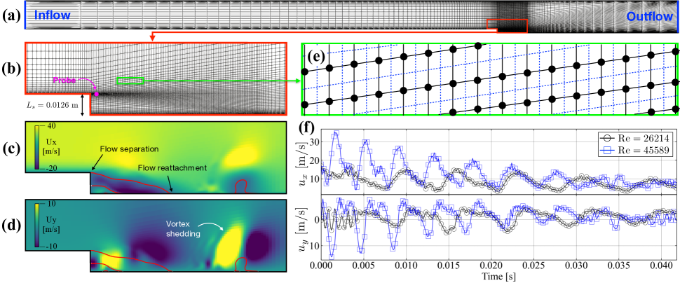
Figure 2: (a) Full mesh of BFS configuration. An inflow boundary condition is provided at the left end, and an outflow at the right. Remaining boundaries are no-slip walls. (b) Zoom-in of the mesh in the near-step region, highlighting the variation in cell size and refinement zones. (c) Instantaneous snapshot of streamwise component of mesh-based velocity field ($U_{x}$) from the $Re=26,214$ trajectory. Red contour marks locations where streamwise velocity is zero. (d) Same as (c), but for vertical velocity component ($U_{y}$). (e) Subset of the finite-volume based graph, which is the dual of the mesh. Black markers are nodes (cell centroids), black lines are edges, and blue dashed lines indicate the underlying mesh cells. (f) Streamwise (top) and vertical (bottom) velocity component evolution at the near-step probe location indicated in (b). Black circles denote Re=26214, blue squares denote Re=45589.

Ground-truth data is generated using computational fluid dynamics (CFD) simulations, which solve a filtered version of the incompressible Navier-Stokes equations on the two-dimensional mesh (CFD details provided in Appendix). Simulations are performed for a range of Reynolds numbers from 26000 to 46000 – Fig. 3 illustrates the organization of each simulation in terms of GNN training and testing data. Each simulation generates a high-dimensional trajectory in time, which is represented as a set of successive instantaneous mesh-based flow snapshots sampled at a fixed time step interval. Figs. 2(c) and (d) show the streamwise and vertical velocity component fields composing one such instantaneous snapshot, sourced from an Re=26,214 simulation. Indicated in the figures are the three characteristic flow features of the BFS geometry: (1) flow separation upon encountering the step, (2) flow re-attachment at the bottom-most wall, and (3) vortex shedding induced by the emergence of recirculation zones in the near-step region. These interacting features emerge from the high degree of nonlinearity in the governing equations at the Reynolds numbers considered here. Since the flow is unsteady, the spatial locations of each of these features (i.e., the flow reattachment point) change as a function of time in accordance to a characteristic vortex shedding cycle, which itself is dependent on the Reynolds number. This unsteadiness and Reynolds number dependence is highlighted in Fig. 2(f), which showcases the temporal evolution of the flow at a single spatial location in the mesh for two Reynolds numbers.

In this work, graphs are generated using a dual mesh interpretation, with each mesh-based snapshot representing an undirected graph with 20540 nodes and 81494 edges. In this interpretation, graph nodes coincide with centroids of computational cells, and edges are formed by connecting neighboring cell centroids such that they intersect shared cell faces. This coincides with numerical stencils used in finite volume (FV) methods of CFD [28]. A visualization of the graph is provided in Fig. 2(e), showing the BFS mesh overlaid on top of a subset of the nodes and edges.

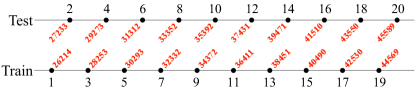
Figure 3: Description of dataset. Each marker denotes a trajectory with ID given in black text, and Reynolds number in red text. Unstructured snapshots for each trajectory correspond to the mesh shown in Fig. 2(a). Each trajectory is comprised of $419$ snapshots separated by $\Delta t=10^{-4}s$.

Combined with the connectivity $E$, input node attribute matrices used for GNN training are recovered directly from the velocity field stored on cell centroids. Since the flow at a particular Reynolds number is unsteady, these fluid velocities are time-evolving, so the features stored in the node attribute matrix can also be considered time-evolving. At a particular time step $m$ along the trajectory, the node attribute matrix is given by

$${\bf X}_{m}=\begin{bmatrix}u(x_{1},m\Delta t)&v(x_{1},m\Delta t)\\ u(x_{2},m\Delta t)&v(x_{2},m\Delta t)\\ \vdots&\vdots&\\ u(x_{|V|},m\Delta t)&v(x_{|V|},m\Delta t)\end{bmatrix},\quad m=1,\ldots,T.$$ (1)

In Eq. 1, $u$ and $v$ denote streamwise and vertical velocity components respectively, $x_{i}$ ($i=1,\ldots,|V|$) is the physical space location for node $i$, $m$ denotes the temporal index, $\Delta t$ is the trajectory time step, and $T$ is the total number of flow snapshots in the trajectory. A trajectory is defined as

$$\mathcal{T}_{n}=({\bf X}_{1},{\bf X}_{2},\ldots,{\bf X}_{T})_{n},\quad n=1,\ldots,20,$$ (2)

where $n$ denotes the trajectory index corresponding to a particular Reynolds number. As shown in Fig. 3, there are a total of 20 trajectories with 10 allocated for training and the remaining 10 for testing.

The GNN architectures introduced in this work operate under the context of mesh-based surrogate modeling. More specifically, the modeling task is

$${\cal G}_{\theta}({\bf X}_{m},{\bf E},E)={\bf S}\approx{\bf X}_{m+1}-{\bf X}_{m},$$ (3)

where ${\cal G}_{\theta}$ denotes a graph neural network described by parameter set $\theta$ and ${\bf S}$ is the GNN prediction. The prediction ${\bf S}$ physically represents the rate-of-change of the velocity field at a fixed timestep $\Delta t$ implicitly prescribed by the training data – the model $\cal G$ can then be used to make forecasts through a residual update via

$$\widetilde{{\bf X}}_{m+1}={\cal G}_{\theta}({\bf X}_{m},{\bf E},E)+{\bf X}_{m}.$$ (4)

Given successive snapshot pairs $({\bf X}_{m},{\bf X}_{m+1})$ extracted from the trajectories ${\cal T}_{n}$, backpropagation-based supervised GNN training can be accomplished by casting objective functions either in terms of the rates ${\bf X}_{m+1}-{\bf X}_{m}$ or the predicted mesh-based flowfield ${\bf X}_{m+1}$ directly. The latter approach is leveraged here, producing the mean-squared error (MSE) based objective function

$${\cal L}_{\text{MSE}}=\left\langle\frac{1}{|V|\times N_{F}}\sum_{i=1}^{|V|}\sum_{j=1}^{N_{F}}({\bf X}^{(i,j)}_{m+1}-\widetilde{{\bf X}}^{(i,j)}_{m+1})^{2}\right\rangle.$$ (5)

Equation 5 represents the single step squared-error in the GNN prediction averaged over the $|V|$ nodes and the $N_{F}$ target features stored on each node ($N_{F}=2$ for the two velocity components considered). The angled brackets $\langle.\rangle$ represent an average over a batch of snapshots (i.e., a training mini-batch). The goal of the baseline training procedure is to optimize GNN parameters $\theta$ such that the MSE loss function in Eq. 5, aggregated over all training points, is minimized. Additional details on the training procedure are provided in the Appendix.

Given this optimization goal, it should be noted that the modeling task in Eq. 4 is challenging by design and deviates from previous mesh-based modeling efforts for a number of reasons:

1. Large GNN timestep: The flow snapshots in the ${\cal T}_{n}$ trajectories are sampled at a fixed GNN timestep $\Delta t$, which is configured here to be significantly larger than the CFD timestep $\delta t$ used to generate the data. When generating the data, the CFD timestep $\delta t$ is chosen to satisfy a stability criterion determined from the numerics used in the PDE solution procedure. Since the ratio $\Delta t/\delta t$ is high (the ratio is 100 here), the GNN is forced to learn a timescale-eliminating surrogate that is much more nonlinear and complex than the $\Delta t=\delta t$ counterpart, particularly in the high Reynolds numbers regime. The tradeoff is that fewer GNN evaluations are required to generate predictions at a target physical horizon time.

2. Absence of pressure: The Navier-Stokes equations, which are the governing equations for fluid flow, identify the role of local pressure gradients on the evolution of fluid velocity. The GNN in Eq. 4, however, operates only on velocity field data, and does not explicitly include pressure or its gradients in the evaluation of dynamics. Instead, the model is tasked to implicitly recover the effect of pressure on the flow through data observations. This is consistent with real-world scenarios in which time-resolved velocity data is accessible (e.g., through optical flow [29] or laser-based imaging [30]), but pressure field data (particularly pressure gradient data) is inaccessible or sparse.

3. Mesh irregularity: The mesh from which the graph is derived (Fig. 2(a)) contains regions of high cell skewness and irregularity, particularly in the far-field regions. Since regression data are sampled directly from cell centers, node neighborhoods near irregular mesh regions are characterized by a high variation in edge length scales. Such irregularities are included here to emphasize the model’s inherent compatibility with unstructured grids.

3 Results

3.1 Fine-Tuning GNNs for Interpretability

It is assumed that a black-box graph neural network optimized for the above described forecasting task – termed the baseline GNN, ${\cal G}_{B}$ – is available. With ${\cal G}_{B}$ as the starting point, the fine-tuning procedure (to be described and demonstrated in this section) produces a new GNN – termed the fine-tuned GNN, ${\cal G}_{F}$ – that is both physically interpretable and optimized for the same modeling task as the baseline ${\cal G}_{F}$. These interpretability properties are embedded into the baseline through architectural modifications; more specifically, ${\cal G}_{F}$ is created by appending ${\cal G}_{B}$ with an interpretable fine-tuning module that does not modify the baseline parameters. The module provides interpretability through a learnable pooling operation that adaptively isolates a subset of nodes in the context of the mesh-based forecasting task (the objective function in Eq. 5). It will be shown how these nodes can be readily visualized to extract coherent physical features most relevant to this forecasting goal, all while while retaining the architectural structure and predictive properties of the baseline model. This approach is illustrated in Fig. 1.

3.1.1 Baseline GNN

The baseline GNN architecture (Fig. 1, top) follows the encode-process-decode strategy [8], which is a leading configuration for data-driven mesh-based modeling. Here, in a first step, input node and edge features – which correspond to velocity components and relative physical space distance vectors, respectively – are encoded using multi-layer perceptrons (MLPs) into a hidden channel dimension, where $N_{H}$ is typically much larger than $N_{F}$, the input feature space size. The result is a feature-encoded graph characterized by the same adjacency matrix as the input graph. This encoded graph is then passed to the processor, which contains a set of $L$ independently parameterized message passing layers that operate in the fixed hidden node and edge dimensionality $N_{H}$.

Message passing layers can take various forms and are the backbone of all GNN architectures, since they directly leverage the graph connectivity to learn complex functions conditioned on the arrangement of graph nodes in neighborhoods [7]. The processor in the baseline architecture in Fig. 1 is a general description, in that the fine-tuning procedure is not tied down to the type of MP layer used. Here, all MP layers correspond to multiscale message passing (MMP) layers, which leverage a series of coarse grids in the message passing operation to improve neighborhood aggregation efficiency [12, 26, 11]. Details on the MMP layer used here can be found in the Appendix, and follow the implementation in Ref. [26].

3.1.2 Interpretable Fine-Tuning Module

The interpretable fine-tuning module is shown in Fig. 1 (bottom), and contains a separate set of layers designed to enhance interpretability properties of the black-box baseline. The module is implemented through a skip connection between the first and last MP layers in the baseline processor block, such that module parameters are informed of the action of baseline neighborhood aggregation functions during parameter optimization. There are three components to the module: an adaptive graph pooling layer, an additional MMP layer that acts on the pooled graph representation, and a parameter-free un-pooling layer.

Interpretability comes from the graph pooling layer, which uses an adaptive node reduction operation as a mechanism for graph dimensionality reduction. This is accomplished using a Top-K based projection-truncation operation [31], illustrated in Fig. 4. In a first step, the input node attribute matrix is reduced feature-wise to a one-dimensional feature space using a projection vector that is learned during training, which constitutes the parameter of the Top-K layer. In a second step, the nodes in this feature space are sorted in descending order; nodes corresponding to the first $K$ values in the reduced feature space are retained, and the remaining nodes are discarded. The node reduction factor, given by the integer $RF=|V|/K$, is a hyperparameter indicating the degree of dimensionality reduction achieved by the Top-K operation: a higher $RF$ means fewer nodes are retained. The truncation procedure produces a sub-graph coincident with a subset of nodes and edges in the original graph. That is, the retained nodes are a subset of $V$, and the edges belonging to these nodes are a subset of $E$. The MMP layer in the module acts on the neighborhoods in this sub-graph, the output of which is un-pooled and sent back to the baseline processor using a residual connection.

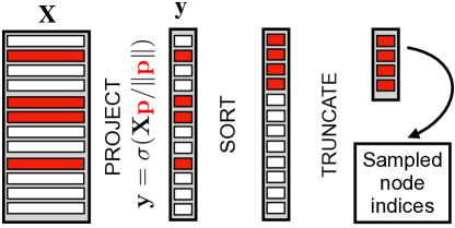
Figure 4: Schematic of Top-K reduction procedure. ${\bf X}\in\mathbb{R}^{|V|\times N_{F}}$ denotes an input node attribute matrix, and ${\bf y}=\sigma({\bf X}{{\bf p}}/\lVert{{\bf p}}\rVert)\in\mathbb{R}^{|V|\times 1}$ is the result of the node-wise projection operation, where ${\bf p}\in\mathbb{R}^{N_{F}\times 1}$ is learned during training and $\sigma$ is a hyperbolic tangent activation function.

As illustrated in Fig. 1, the sub-graph produced by the pooling layer can be readily visualized in a mesh-based setting, since the extracted nodes correspond to locations in physical space. If the predictive capability of the baseline is withheld when optimizing the parameters in the interpretable module, nodes identified in the sub-graphs serve as an accessible link to the forecasting task. The discussion below shows how adaptive node sub-sampling provided by the pooling operation identifies physically coherent artifacts in the mesh-based domain, thereby connecting the data-based modeling task (the goal of the baseline) with application-oriented features of interest (the goal of the interpretable fine-tuning module).

3.1.3 Fine-tuning Procedure

Fine-tuning is accomplished by first initializing the ${\cal G}_{F}$ model parameters directly from those in the baseline ${\cal G}_{B}$, which is assumed to already have been trained. Then, the interpretable module is appended to the ${\cal G}_{F}$ architecture as per Fig. 1.

A training step for ${\cal G}_{F}$ is then carried out using the same objective function used to train the baseline ${\cal G}_{B}$. During training, the subset of parameters in ${\cal G}_{F}$ corresponding to the baseline is frozen, and the parameters corresponding to the interpretable module are freely trainable. This ensures that the fine-tuned GNN parameters include the baseline parameters as a subset, and isolate optimization focus to the interpretable module parameters during training; in other words, if the baseline parameters are kept frozen, the adaptive pooling layer is forced to identify sub-graphs that result in improved baseline accuracy from the perspective of the objective function being optimized (in this case, a single-step forecast). The fine-tuning procedure is shown in Fig. 5, which displays objective function optimization histories for fine-tuned GNNs trained with different values of node reduction factor $RF$.

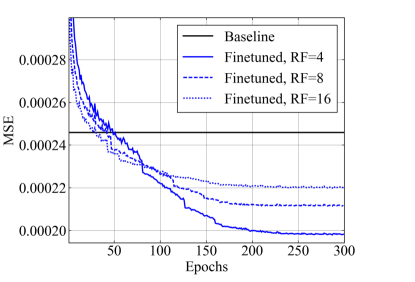
Figure 5: Mean-squared error objective (Eq. 5) versus training epochs during fine-tuning phase.

The training histories show two key trends: (1) the baseline objective history is frozen, as the baseline model ${\cal G}_{B}$ is not being modified, and (2) the fine-tuned models achieve lower converged mean-squared errors in single-step GNN predictions than the baseline. The latter trend is consistent with the fact that additional parameters are introduced in the fine-tuning procedure (see Fig. 1). Due to the fact that a message passing layer acts on the Top-K-identified subgraphs, the converged training errors increase with decreasing RF. Higher RF translates to sub-graphs occupying a smaller percentage of original graph nodes, which in turn limits the scope of the additional message passing layer.

3.1.4 Masked Fields

The interpretability enhancement provided by the fine-tuning procedure is illustrated in Fig. 6, which contrasts the single-step prediction workflow of the baseline GNN with that of a series of fine-tuned GNNs, each having incrementally higher values of RF. The input to all models is the same instantaneous mesh-based flowfield ${\bf X}_{m}$ sourced from a testing set trajectory.

Figure 6 shows how the fine-tuning procedure adds masked fields to the model evaluation output. Simply put, a masked field is generated by visualizing the sub-graph node indices produced by the Top-K pooling operation. Since these truncated nodes coincide with physical space locations consistent with the underlying mesh, the “active” nodes selected during pooling can be extracted and visualized as a node-based categorical quantity (1 if the node was identified and 0 otherwise).

The features contained in these fields allow one to interpret the relationship between the input flow field ${\bf X}_{m}$ and the model-derived forecast $\widetilde{\bf X}_{m+1}$. In other words, through visualization of the masked fields, the fine-tuned models allow one to access regions in physical space intrinsically linked to the modeling task (single-step prediction), thereby making the model behavior directly accessible from the perspective of the objective function used during training. The masked fields in Fig. 6 show how this added capability translates to interpretable prediction unavailable in the baseline, as the masked fields interestingly isolate nontrivial, but spatially coherent, clusters of nodes (often disjoint in physical space) within the GNN forward pass. Such features can then be connected to the problem physics in an expert-guided analysis phase.

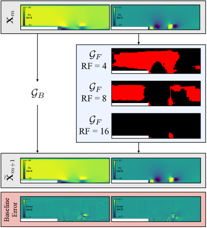
Figure 6: Comparison of GNN prediction workflows between baseline and fine-tuned GNNs. Fine-tuned workflow includes masked fields generated in forward pass. Input flowfield (top) sourced from Re=27,233 trajectory of the testing set. Bottom-most plots show baseline absolute error fields ($\widetilde{\bf X}_{m+1}-{\bf X}_{m+1}$) for streamwise (left) and vertical (right) velocity components.

For example, as the reduction factor increases, the masked fields in Fig. 6 isolate coherent regions corresponding to near-step recirculation zones and downstream vortex shedding. In particular, the increase in $RF$ emphasizes importance of the step cavity region in the forecasting task – the emphasis on the free-stream region in the masked field drops, implying that the role played in the step cavity region is much more important when making accurate model forecasts. This trend is expected in the BFS configuration, and is overall consistent with the fact that high baseline model errors are also observed in this region.

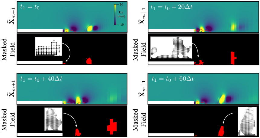
Figure 7: Single-step prediction outputs generated by fine-tuned GNN (RF=16) using input fields at time-ordered instants in the Re=27233 trajectory. Each frame shows predicted y-component of velocity (top) alongside masked field (bottom), with inlays showing subgraph representations.

Since the input velocities stored on the nodes are time-evolving, and the Top-K projection operation is conditioned on these input values, the regions identified in the masked fields are necessarily time-evolving as well. Consequently, the masked fields identify coherent structures that evolve in accordance with the unsteady features of the flow – in the BFS configuration, these features correspond to emerging and downstream shedding of recirculation zones, which in turn lead to a shedding cycle that affects the location at which the flow reattaches to the bottom wall. This time-dependent quality is highlighted in Fig. 7, which shows a set of time-ordered single-step predictions paired with corresponding masked fields during one BFS shedding cycle. It should be noted that the adaptive pooling operation induces a sub-graph from which the masked field is derived; since the identified regions in the masked fields are time-evolving, the adjacency matrix that characterizes this sub-graph is time-evolving as well, and remains coincident with the fixed adjacency matrix of the original mesh-based graph. The sub-graphs are provided as inlaid plots in Fig. 7; these evolving adjacency matrices enable successive utilization of MMP layers on these isolated regions in the fine-tuned model.

3.1.5 Preserving baseline performance

Incorporation of the interpretability enhancement does not come for free, and incurs the following costs: (1) there is an additional offline training step due to fine-tuning; and (2) inference of the fine-tuned models is more costly compared to their baseline counterparts, due to the introduction of an additional set of arithmetic operations through the interpretable module attachment. In light of these costs, the advantage is that the fine-tuned models not only provide interpretability, but also maintain the performance of the baseline models in terms of forecasting accuracy and stability characteristics.

To emphasize this point, Fig. 8 displays root-mean-squared errors (RMSE) in single-step predictions for baseline and fine-tuned models as a function of testing set Reynolds numbers. The RMSE is calculated node-wise, is computed separately for each predicted output feature, and is normalized by the inlet velocity to allow for relative comparisons across the range of tested Reynolds numbers. More formally, for the $j$-th output feature (the velocity component), it is defined as the relative error percentage

$$\text{RMSE}_{j}=\frac{\left\langle\sqrt{\frac{1}{|V|}\sum_{i=1}^{|V|}({\bf X}^{(i,j)}_{m+1}-\widetilde{{\bf X}}^{(i,j)}_{m+1})^{2}}\right\rangle}{u_{in}}\times 100,$$ (6)

where $\widetilde{{\bf X}}^{(i,j)}_{m+1}$ denotes the single-step GNN prediction for the $j$-th feature at graph node $i$, ${{\bf X}}^{(i,j)}_{m+1}$ is the corresponding target, $u_{in}$ is the inlet velocity corresponding to a particular Reynolds number, and the angled brackets $\langle.\rangle$ denote an ensemble average over testing set samples.

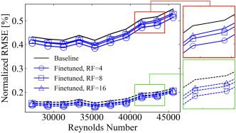
Figure 8: Normalized RMSE (Eq. 6) versus testing Reynolds number for streamwise (solid lines) and vertical (dashed lines) velocity components.

Since the fine-tuning procedure discussed thus far leverages the same objective function as the baseline – namely, the single-step forecasting error in Eq. 5 – the trends in testing set evaluations for this metric are overall consistent with what was observed during training (see Fig. 5). More specifically, Fig. 8 shows how the baseline is effectively an upper bound for the model error at all evaluation Reynolds numbers. Additionally, the error in fine tuned models approaches the baseline as the node reduction factor $RF$ increases. It should also be noted that the normalized error curves are not flat – after about Re=35,000, the relative errors begin to increase, emphasizing the increase in unsteady flow complexity in this regime. This increase is likely an artifact of the fixed timestep using during training. Alongside higher velocity magnitudes fluctuation in the near-step regions, since the shedding cycle frequencies are more rapid at higher Reynolds numbers, the forecasting task becomes more difficult in a given fixed GNN $\Delta t$ window.

Although the averaged single-step error is valuable when validating the consistency between baseline and fine-tuned model outputs in an a-priori setting, comparison of model performance in an a-posteriori (or rollout) setting is required to confirm that the fine-tuning procedure indeed preserves the overall characteristics of the baseline model in a truly predictive context. Such a comparison is given in Fig. 9(a) and (b), which shows rollout predictions for streamwise and vertical velocity components respectively for three different Reynolds numbers. The rollouts are sampled at three fixed spatial (probe) locations in the step cavity region, where the BFS dynamics are most complex: probe 1 is the closest to the step anchor, and reflects the impact of flow separation on the unsteady dynamics, whereas probes 2 and 3 are successively further downstream.

The rollouts ultimately confirm predictive consistency between the fine-tuned GNN and the corresponding baseline – in almost all cases, the predictions provided by the fine-tuned model very closely resemble those of the baseline. Interestingly, the rollouts in Fig. 9 reveal noticeable error buildup in the near-step regions as opposed to further downstream. The degree of error buildup is most prominent at the highest tested Reynolds number, where the onset of instability starts at about 20 rollout steps; this is consistent with the trends in Fig. 8, which implies that accumulation of single-step error is most pronounced at the highest Reynolds numbers.

While the rollout accuracy, particularly near the step, is less than ideal, two important points must be stressed: (a) the GNN timestep $\Delta t$ is prescribed here to be significantly larger than the CFD timestep (as discussed in the previous section); and (b) error accumulation is expected since the objective function used during training and fine-tuning only accounts for the single-step error. Although inclusion of multiple rollout steps during training has been shown in recent work to significantly improve GNN prediction horizons for baseline models [6], such investigations into long-term stability improvements were not explored in this work, as they significantly increase training times and require complex application-specific training schedules. Since the scope of this work is interpretable fine-tuning with respect to a baseline, the objective of Fig. 9 is to highlight how appending the interpretable fine-tuning module to the baseline GNN does not incur significant accuracy penalties in both single-step and rollout contexts. As a result, it can be concluded that the added benefit of masked field interpretability is a meaningful addition to the black-box model.

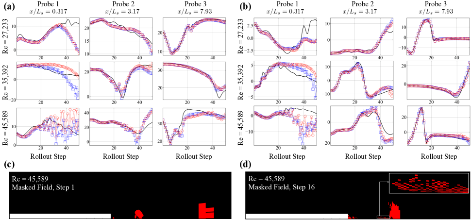
Figure 9: (a) Rollout predictions for streamwise velocity component at fixed probe locations for baseline GNN (blue squares) and fine-tuned GNN (RF=16, red circles). Solid black line indicates target value. Rows correspond to different initial conditions sourced from the indicated Reynolds numbers; columns correspond to different probe locations at specified x-locations away from step anchor (y-locations of probes coincide with the step height). (b) Same as (a), but for vertical velocity component. (c) Masked field after 1 rollout step for Re=45,589. (d) Masked field after 16 rollout steps for Re=45,589; inlay shows zoom-in on a portion of the masked field.

Figure 9(c) and (d) provide masked field visualizations from the Re=$45,589$ predictions produced by the fine-tuned GNNs, and show the effect of rollout error accumulation on the masked field structures. More specifically, the masked field at the first rollout step in Fig. 9(c) isolates largely coherent structures in the step cavity, as observed in the previous examples (see Fig. 7), whereas the masked field after 16 rollout steps (Fig. 9(d)) includes the emergence of high frequency checkerboard-like patterns that are largely non-physical. These visualizations show a direct correspondence between rollout errors and spatial coherency observed in the identified masked field structures – although more investigation to this end is required, the advantage is that the masked field is generated directly by the model during inference, and it is possible that such high-frequency artifacts can be used to signal oncoming model error accumulation in an a-posteriori context.

3.2 Error-Identifying GNNs

The results described in Sec. 3.1 showcased the interpretability enhancement provided by the fine-tuned model from the angle of feature extraction. More specifically, the structures identified by the fine-tuned GNNs through the masked fields serve as an accessible link between the model architecture and the optimization goal (the mesh-based flow forecast).

The goal of this section is to build on the above by adding more capability to the identified masked fields from the modeling perspective (i.e., providing utility beyond feature extraction). This is accomplished by adding a regularization term, representing a mean-squared error budget, to the objective function during the fine-tuning process. It is shown below how the inclusion of this relatively simple regularization forces the identified nodes in the masked field to not only produce coherent features, but also to coincide with regions that contribute most significantly to the fine-tuned GNN forecasting error, a capability not guaranteed in the standard fine-tuning procedure.

This strategy is inspired from error tagging methods leveraged in adaptive mesh refinement (AMR) based CFD solvers [32], in which the first step consists of tagging subset of mesh control volumes expected to contribute most to the PDE discretization error. In AMR strategies, knowledge of error sources in discretization methods used to solve the Navier-Stokes equations is used to guide which regions are tagged (for example, regions containing high gradients in pressure and fluid density); since the baseline GNN forecasting model is considered a black-box, the goal here is to offer an analogous data-based pathway that isolates sub-graphs in input graphs processed by GNNs coinciding with regions of high model error. Such information adds error-tagging utility to the masked fields, which can then be used to guide downstream error-reduction strategies.

3.2.1 Budget Regularization

The budget regularization strategy is accomplished by modifying the objective function used during the fine-tuning procedure. This modified objective function adds a regularization term to the standard single-step prediction objective of Eq. 5, and is given by

$${\cal L}_{R}={\cal L}_{\text{MSE}}+\lambda{\cal L}_{B},$$ (7)

where ${\cal L}_{R}$ denotes the regularized loss, ${\cal L}_{\text{MSE}}$ denotes the mean-squared error based forecasting objective in Eq. 5, $\lambda$ is a scaling parameter, and ${\cal L}_{B}$ is the so-called budget regularization term given by

$${\cal L}_{B}=\frac{1}{\langle{\cal B}\rangle},\quad{\cal B}=\frac{\sum_{i=1}^{|V|}\sum_{j=1}^{N_{F}}{\bf M}_{m}^{i}({\bf X}^{(i,j)}_{m+1}-\widetilde{{\bf X}}^{(i,j)}_{m+1})^{2}}{\sum_{i=1}^{|V|}\sum_{j=1}^{N_{F}}({\bf X}^{(i,j)}_{m+1}-\widetilde{{\bf X}}^{(i,j)}_{m+1})^{2}}.$$ (8)

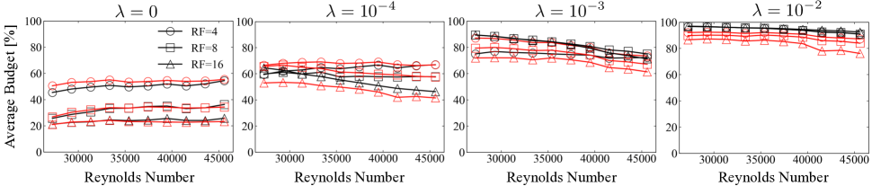
Figure 10: Average masked field budgets (Eq. 8) versus testing Reynolds number produced by fine-tuned GNNs using increasing values of $\lambda$. Black curves correspond to streamwise velocity component, and red to vertical velocity component.

In Eq. 8, the quantity ${\cal B}$ is the masked field budget, and represents the contribution to the total mean-squared error for the single-step forecast from the nodes identified in the masked field ${\bf M}_{m}^{i}$, where the subscript $m$ denotes dependence on the input flowfield at the $m$-th time step (${\bf X}_{m}$), and the superscript $i$ indexes a node in the graph. As per the definition of the masked field, ${\bf M}_{m}^{i}$ is 1 if the node is identified through the Top-K pooling procedure, and 0 otherwise. Since the regularization term ${\cal L}_{B}$ is cast as the inverse of the budget ${\cal B}$, a model with a small value of ${\cal L}_{B}$ indicates that a large amount of forecasting error is contained in the nodes identified through the masked field. The parameter $\lambda$ in Eq. 7 dictates the influence of the regularization term during the fine-tuning stage, and therefore plays a critical role. Note that the setting $\lambda=0$ recovers the non-regularized fine-tuning strategy discussed throughout Sec. 3.1. Through the dependence of ${\cal B}$ on the masked field, the objective is to ensure that – if the regularization strategy succeeds in reducing ${\cal L}_{B}$ – the nodes responsible for a majority of the forecasting error are accessible as an explicit function of the input mesh-based flowfield ${\bf X}_{m}$, resulting in a type of a-posteriori error tagging strategy.

3.2.2 Impact of Regularization

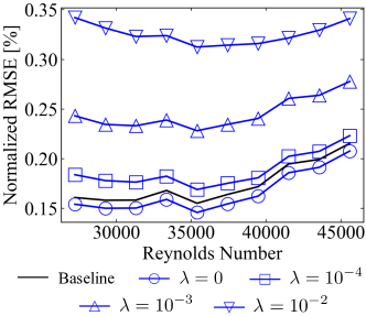
Figure 11: Normalized RMSE (Eq. 6) versus testing Reynolds number for baseline GNN (black) and fine-tuned GNNs trained with different levels of budget regularization scaling factor $\lambda$ (markers). All fine-tuned GNNs in figure use $RF=16$. RMSE curves shown for vertical velocity component (trends are consistent for streamwise component).

The effect of the scale factor $\lambda$ on the budget-regularized fine-tuning is shown in Fig. 10, which plots average budget values (single-step prediction error contained in the masked fields) conditioned on both testing set Reynolds number and velocity component for various fine-tuned GNN configurations. The figure illustrates (a) how various degrees of error tagging capability are indeed being provided through the budget regularization procedure in direct proportion to $\lambda$, and (b) the expected relationship between the node reduction factor and budget (higher $RF$ gives lower budget contributions). For example, the standard fine-tuning strategy corresponding to $\lambda=0$ produces masked fields that describe a noticeably lower amount of model error than the regularized ($\lambda>0$) counterparts. Interestingly, the implication is that without budget regularization, the generated masked fields – even for a relatively large node reduction factor of $RF=4$, meaning that $25\%$ of the total nodes are sampled – account for only roughly half of the forecasting error contribution. On the other hand, as $\lambda$ is progressively increased from $10^{-4}$ to $10^{-2}$, the budget values increase across the board. The $\lambda=10^{-2}$ case nearly reaches a saturation point, where a majority of the single-step forecasting error in most cases is described by the identified nodes. The budget curves are almost flat, with some exceptions at the higher tested Reynolds numbers, implying that the regularization strategy learning a robust and interpretable error-identifying mechanism.

Although the increase in $\lambda$ translates to an increase in error-identifying capability in the fine-tuned GNNs, Figure 11 shows how the regularization incurs an accuracy tradeoff. More specifically, Fig. 11 shows effect of the $\lambda$ parameter on the fine-tuned GNNs in terms of single-step normalized RMSE values (Eq. 6) conditioned on the same testing set Reynolds numbers. When the budget regularization is introduced, the scaling parameter effectively increases the forecasting errors for all observed Reynolds numbers, implying a type of accuracy tradeoff with respect to the additional modeling capability provided by the budget regularization. This is overall consistent with the $\lambda$-scaling process, in that a greater emphasis on minimizing the inverse budget via high $\lambda$ necessitates less optimization focus on the direct forecasting error objective. This attribute is directly apparent in Fig. 11 – as $\lambda\rightarrow 0$, the RMSE curves converge to the standard fine-tuned GNN, which achieves lower forecasting error relative to the baseline GNN used to initiate the fine-tuning procedure.

To further assess the effect of budget regularization in a more practical inference-based setting, Fig. 12 displays forecasting results in terms of masked field budget and predicted velocity versus time step using an initial condition sourced from the Re=35,392 testing set trajectory. The figure compares fine-tuned GNN forecasts in single-step and rollout prediction configurations, with models corresponding to node reduction factors (RFs) of 16 (the adaptive pooling procedure isolates sub-graphs comprised of 16x fewer nodes than the original).

The single-step forecasts largely mimic the trends observed in Fig. 10, in that the regularization imposed during fine-tuning manifests through an increase in error budget during inference with higher $\lambda$. These single-step forecasts, which assume no accumulation of model forecasting error through forward time steps, highlight the control provided by the regularization procedure by the $\lambda$ parameter. More specifically, Fig. 12 indicates diminishing returns in the regularization procedure with respect to $\lambda$: for example, the jump in budget when moving from $\lambda=0$ to $\lambda=10^{-4}$ is on average higher than when moving from $\lambda=10^{-3}$ to $\lambda=10^{-2}$. The rollout trends, which do account for the accumulation of single-step forecasting error through trajectory generation, further point to this aspect of diminishing returns, and directly reveal how the added emphasis on budget regularization through higher $\lambda$ values incurs an accuracy tradeoff. For example, the fine-tuned GNN trained with $\lambda=10^{-2}$ departs from the target solution much earlier than the others, which is consistent with the fact that it places more emphasis on minimizing the inverse budget during fine-tuning – ultimately, the cost of having a more ”useful” masked field through the ability to tag regions of high error is a drop in forecasting accuracy and stability. Interestingly, although the correlation between budget and the $\lambda$ parameter is present for the first few rollout steps, this correlation decays once error starts to pollute the predictions. In other words, the budgets in the regularized models eventually tend towards the budgets produced by the non-regularized model. Since the baseline and fine-tuning procedures utilize single-step training objectives, the impact of error accumulation after a single forecasting step is high – as mentioned earlier, these effects can be mitigated with more robust (albiet more expensive) training strategies that account for the error of more than one future time-step in the objective function.

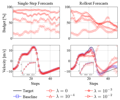
Figure 12: (Top row) Masked field budgets (Eq. 8) versus time step for single-step (left plot) and rollout (right plot) predictions using initial condition from Re=35,392 testing set trajectory. Fine-tuned GNNs have RF=16. (Bottom row) Corresponding velocity field predictions (vertical component) sampled at a single spatial location (probe 2, same as used in middle row of Fig. 9(b)).

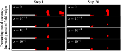
Figure 13: (Left) Masked fields (Sec. 3.1.4) produced by fine-tuned GNNs of varying $\lambda$ settings after 1 rollout step, for same trajectory described in Fig. 12. (Right) Corresponding masked fields after 10 rollout steps.

It should be noted that for small values of $\lambda$ (e.g., $\lambda=10^{-4}$ in Fig. 12), the regularization in Eq. 7 produces error-identifying masked fields at relatively minimal expense in terms of model accuracy with respect to the baseline GNN, thereby offering a unique interpretable modeling advantage from the perspective of error tagging. This advantage is more apparent when considering Fig. 13, which shows masked fields produced by the fine-tuned GNNs used to make the predictions in Fig. 12. The introduction of $\lambda$ incurs a noticeable change to the identified structures in the masked field; more specifically, the non-regularized $\lambda=0$ fine-tuned GNNs isolate structures in the far downstream region, whereas the regularized models isolate more nodes in the near-step vicinity, particularly near the corner at which flow separation is initiated. The difference in masked field structures emphasizes the difference in GNN fine-tuning objectives, in that the identified nodes in the $\lambda>0$ models represent regions in which the predicted mesh-based flowfield $\widetilde{X}_{m+1}$ will contain a majority of the model error. Additionally, the structures in the masked fields from $\lambda=10^{-4}$ to $\lambda=10^{-2}$ are largely similar, which allows the user to tune the degree of error identification capability provided by the fine-tuned GNN. For example, the $\lambda=10^{-4}$ model offers (a) comparable performance to the baseline GNN, (b) interpretability through the identification of coherent structures in the masked field, a utility also provided in the non-regularized $\lambda=0$ model, and (c) the ability to attribute the identified regions to expected sources of forecasting error. Although this latter capability is limited to the scope of the prediction horizon of the model (this is apparent through the rollout results in Fig. 12), the inclusion of the budget-based regularization reveals a promising pathway for understanding and isolating sources of model error during inference through the adaptive pooling strategy.

4 Discussion

This work introduces an interpretable fine-tuning strategy for graph neural network based surrogate models, with focus on unstructured grid based fluid dynamics. More specifically, given a baseline GNN, the fine-tuning strategy consists of (a) appending an interpretable module to the GNN architecture through a skip connection, and (b) an isolated training stage to optimize the parameters introduced by this appended module. The resultant fine-tuned GNN adds interpretability to the baseline GNN by means of a graph pooling layer that acts as an adaptive sub-graph sampler, where these sub-graphs are identified in accordance to the underlying objective function (which here is the mesh-based forecasting error). Through this pooling operation, it is shown how the GNN forward pass generates masked fields as a by-product, which isolates regions in physical space in which these sampled sub-graphs are active. The features contained in these masked fields allow one to interpret the relationship between the input flow field at the current time instant, and the model-derived forecast at a future time instant. Through visualization of the masked fields, the fine-tuned GNNs allow one to access regions in physical space intrinsically linked to the modeling task (forecasting), thereby making the model behavior directly accessible from the perspective of the objective function used during training. As a result, the structures identified by pooling operation serve as an accessible link between the forecast-based objective function, the baseline model architecture, and the underlying physics of the problem being modeled.

Additionally, by adding a regularization term to the objective function during the fine-tuning procedure in the form of an error budget, it was shown how the mask fields can also be used to identify, during inference, nodes that describe a majority of the anticipated forecasting error. Since the masked fields are an explicit function of the input flowfield (and not the predicted future flowfield), this regularization step adds a form of interpretable error-tagging capability to the modeling framework.

The authors believe that the fine-tuning strategies introduced here begin to address the limitations of existing black-box mesh-based modeling strategies, and can readily be extended to other applications both within and outside of fluid dynamics surrogate modeling. For example, the objective functions studied here concentrated on single-step forecasting errors – an interesting direction for future work is to append the same interpretable fine-tuning module, but include more rollout steps during the fine-tuning process, thereby producing an interpretable stability enhancement. Including physics-based loss terms is another promising direction, as it would allow one to investigate the relationship between the identified structures and governing equation residuals. Additionally, although the modeling context in this work focused on a node-level regression task, the same interpretable module can leveraged for graph-level regression tasks, which would in turn change the identified structures in the masked fields. These aspects, as well as other directions, will be explored in future work.

Appendix

Data Generation

Data was generated using computational fluid dynamics (CFD) simulations of the BFS configuration. Additional geometric detail of the BFS configuration is provided in Fig. 14. The simulations were conducted using OpenFOAM, which is an open-source CFD backend that includes a suite of default fluid flow solvers tailored to various physics applications. OpenFOAM leverages finite-volume discretization using unstructured grid representations. For this work, the PimpleFOAM solver was used, which implements a globally second-order discretization of the unsteady incompressible Navier-Stokes equations [33, 34, 35]. This software is used to solve a filtered version of the two-dimensional Navier-Stokes equations (analogous to large-eddy simulation), written as

$$\begin{split}\frac{\partial\widetilde{u}_{j}}{\partial t}+\frac{\partial\widetilde{u}_{i}\widetilde{u}_{j}}{\partial x_{i}}&=\nu\frac{\partial^{2}\widetilde{u}_{j}}{\partial x_{i}\partial x_{i}}-\frac{\partial\tau_{ij}^{r}}{\partial x_{i}}-\frac{1}{\rho}\frac{\partial\widetilde{p}}{\partial x_{j}},\\ \frac{\partial\widetilde{u}_{k}}{\partial x_{k}}&=0.\end{split}$$ (9)

In Eq. 9, $\widetilde{.}$ denotes a spatial (implicit) filtering operation, ${u}_{j}$ is the time-evolving $j$-th component of velocity, $p$ is the pressure, $\nu$ is a constant kinematic viscosity, $\rho$ is a constant fluid density, and $\tau^{r}$ is the deviatoric component of the residual, or sub-grid scale (SGS), stress tensor. This is represented here using a standard Smagorinsky model [36], which casts the residual stress $\tau_{ij}^{r}$ as a quantity proportional to the filtered rate-of-strain as

$$\begin{split}\tau_{ij}^{r}&=-2\nu_{r}\widetilde{S}_{ij},\\ \nu_{r}&=\left(C_{S}\Delta\right)^{2}|S|.\end{split}$$ (10)

In Eq. 10, $S_{ij}$ is the filtered rate-of-strain, $|S|=\sqrt{2S_{ij}S_{ij}}$ is its magnitude, $\nu_{r}$ is the turbulent eddy-viscosity, $C_{S}$ is the Smagorinsky constant ($C_{S}=0.168$ here), and $\Delta$ is the box-filter width. These simulation parameters, alongside the mesh and boundary condition specifications required to run the simulation, are provided through input files in the OpenFOAM case directory.

Multiscale Message Passing Layer

As illustrated in Fig. 1, the baseline GNN architecture and the fine-tuning module leverage multiscale message passing (MMP) layers. In short, MMP layers invoke a series of standard message passing layers on a hierarchy of graphs corresponding to different characteristic lengthscales. This section briefly outlines the formulation of these layers.

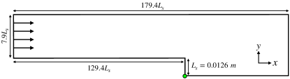
Figure 14: Schematic of BFS geometry (not to scale). Green point indicates grid origin. See Fig. 2 for full mesh to scale.

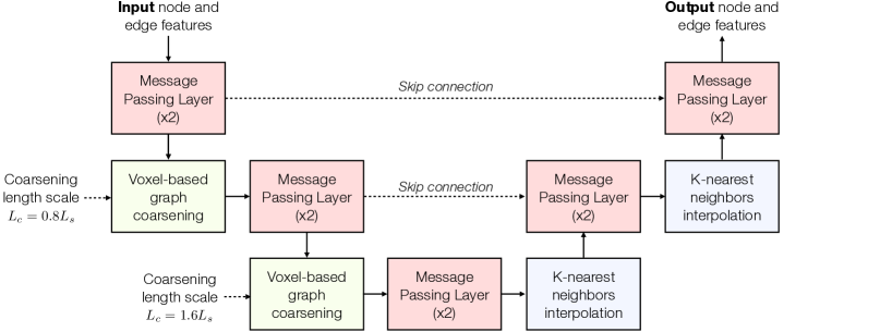
Figure 15: Multiscale message passing (MMP) layer used in baseline and fine-tuned GNN architectures in Fig. 1.

A schematic of the MMP layer architecture used in this work is shown in Fig. 15, and follows the general formulation of the same layer used in Ref. [26]. Note that a single MMP layer in this context can be interpreted as a U-net type architecture. There are three components: (1) single-scale message passing, (2) a graph coarsening operation, and (3) a graph interpolation operation.

Message passing: A message passing layer updates node and edge features without modifying the graph connectivity. One single-scale message passing layer consists of the following operations:

$$\text{Edge update: }{\bf e}_{ij}^{p} ={\cal F}_{e}({\bf e}_{ij}^{p-1},{\bf x}_{i}^{p-1},{\bf x}_{j}^{p-1})\in\mathbb{R}^{N_{H}}$$ (11)

$$\text{Edge aggregation: }{\bf a}_{i}^{p} =\frac{1}{|\mathcal{N}(i)|}\sum_{j\in\mathcal{N}(i)}{\bf e}_{ij}^{p}\in\mathbb{R}^{N_{H}}$$ (12)

$$\text{Node update: }{\bf x}_{i}^{p} ={\cal F}_{n}({\bf a}_{i}^{p},{\bf x}_{i}^{p-1})\in\mathbb{R}^{N_{H}}.$$ (13)

In the above equations, the superscript $p$ denotes the message passing layer index, ${\bf e}_{ij}$ is the edge feature vector corresponding to sender and receiver node indices $i$ and $j$ respectively, ${\bf x}_{i}$ is the feature vector for node $i$, $\mathcal{N}(i)$ is the set of neighboring node indices for node $i$, and ${\cal F}_{e}$ and ${\cal F}_{n}$ are independently parameterized multi-layer perceptrons (MLPs). The quantity ${\bf a}_{i}$ represents the neighborhood-aggregated edge features corresponding to node $i$, and $N_{H}$ is the hidden feature dimensionality (assumed to be the same for nodes and edges after the action of the encoder, see Fig. 1).

Coarsening and Interpolation: As the name implies, the goal of graph coarsening in this context is to coarsen a given input graph such that the average edge lengthscale (in terms of relative distance in physical space) is increased. There are a number of ways to achieve graph coarsening – here, a voxel clustering strategy is used, which produces the coarse graph using voxelization based on an input coarsening lengthscale. Briefly, in this approach, a graph is coarsened by first overlaying a voxel grid, where the centroids of the voxel cells coincide with the coarsened graph nodes. The underlying fine graph nodes can then be assigned to the voxel cells/clusters via computation of nearest centroids, where the coarse node features are initialized using the average of fine node features within a cell. Edges between coarse nodes are added if fine graph edges intersect a shared voxel cell face – the coarse graph edge features are then initialized by averaging fine edge features for edges that satisfy this intersection. For interpolation, a K-nearest neighbors (KNN) strategy is used which amounts to linear interpolation to populate fine node features with a user-specified K number of nearby coarse nodes (K=4 in the MMP layers used in this work). Voxelization and KNN interpolation are implemented using the voxel_grid and knn_interpolate functions available in PyTorch Geometric [37].

Architecture and Training Details

All models in this study were implemented using PyTorch [38] and PyTorch Geometric [37] libraries. Following Fig. 1, a total of 2 MMP layers were utilized in the processor (L=2), the encoder and decoder operations leverage three-layer MLPs, and all message passing layers leverage two-layer MLPs. All MLPs incorporate exponential linear unit (ELU) activation functions with residual connections. Layer normalization [39] is used after every MLP evaluation. The hidden feature dimensionality is set to $N_{H}=128$.

Input node features in ${\bf X}_{m}$ correspond to streamwise and vertical velocity components, target node features are the same features at a future time step ${\bf X}_{m+1}$, and edge features in ${\bf E}$ are initialized using relative physical space distance vectors between the respective nodes. Before training, the data was standardized using training data statistics, and 10% of training data was set aside for validation purposes. As per the findings in Ref. [8], a small amount of noise was injected into the input mesh-based flowfields for stability purposes; each input node feature was perturbed independently by scalar value sampled from a normal distribution with standard deviation of $10^{-2}$ before training.

The Adam optimizer [40] equipped with a plateau-based scheduler (implemented in the PyTorch function ReduceLROnPlateau) was utilized during training with an initial learning rate of $10^{-5}$ and minimium learning rate fixed to $10^{-7}$. The batch size used during training was $8$. Each model was trained using 8 Nvidia A100 GPUs hosted on two nodes of the Polaris supercomputer at the Argonne Leadship Computing Facility.

References

- [1] L. Wu, P. Cui, J. Pei, L. Zhao, X. Guo, Graph neural networks: foundation, frontiers and applications, in: Proceedings of the 28th ACM SIGKDD Conference on Knowledge Discovery and Data Mining, 2022, pp. 4840–4841.
- [2] M. M. Bronstein, J. Bruna, Y. LeCun, A. Szlam, P. Vandergheynst, Geometric deep learning: going beyond euclidean data, IEEE Signal Processing Magazine 34 (4) (2017) 18–42.
- [3] P. W. Battaglia, J. B. Hamrick, V. Bapst, A. Sanchez-Gonzalez, V. Zambaldi, M. Malinowski, A. Tacchetti, D. Raposo, A. Santoro, R. Faulkner, et al., Relational inductive biases, deep learning, and graph networks, arXiv preprint arXiv:1806.01261 (2018).
- [4] J. Jumper, R. Evans, A. Pritzel, T. Green, M. Figurnov, O. Ronneberger, K. Tunyasuvunakool, R. Bates, A. Žídek, A. Potapenko, et al., Highly accurate protein structure prediction with alphafold, Nature 596 (7873) (2021) 583–589.
- [5] M. Eliasof, E. Haber, E. Treister, Pde-gcn: Novel architectures for graph neural networks motivated by partial differential equations, Advances in neural information processing systems 34 (2021) 3836–3849.
- [6] R. Lam, A. Sanchez-Gonzalez, M. Willson, P. Wirnsberger, M. Fortunato, A. Pritzel, S. Ravuri, T. Ewalds, F. Alet, Z. Eaton-Rosen, et al., Graphcast: Learning skillful medium-range global weather forecasting, arXiv preprint arXiv:2212.12794 (2022).
- [7] J. Gilmer, S. S. Schoenholz, P. F. Riley, O. Vinyals, G. E. Dahl, Neural message passing for quantum chemistry, in: International conference on machine learning, PMLR, 2017, pp. 1263–1272.
- [8] T. Pfaff, M. Fortunato, A. Sanchez-Gonzalez, P. W. Battaglia, Learning mesh-based simulation with graph networks, arXiv preprint arXiv:2010.03409 (2020).
- [9] F. D. A. Belbute-Peres, T. Economon, Z. Kolter, Combining differentiable pde solvers and graph neural networks for fluid flow prediction, in: international conference on machine learning, PMLR, 2020, pp. 2402–2411.
- [10] Z. Yang, Y. Dong, X. Deng, L. Zhang, Amgnet: Multi-scale graph neural networks for flow field prediction, Connection Science 34 (1) (2022) 2500–2519.
- [11] M. Lino, S. Fotiadis, A. A. Bharath, C. D. Cantwell, Multi-scale rotation-equivariant graph neural networks for unsteady eulerian fluid dynamics, Physics of Fluids 34 (8) (2022).
- [12] M. Fortunato, T. Pfaff, P. Wirnsberger, A. Pritzel, P. Battaglia, Multiscale meshgraphnets, arXiv preprint arXiv:2210.00612 (2022).
- [13] J. Xu, A. Pradhan, K. Duraisamy, Conditionally parameterized, discretization-aware neural networks for mesh-based modeling of physical systems, Advances in Neural Information Processing Systems 34 (2021) 1634–1645.
- [14] Y. Salehi, D. Giannacopoulos, Physgnn: A physics–driven graph neural network based model for predicting soft tissue deformation in image–guided neurosurgery, Advances in Neural Information Processing Systems 35 (2022) 37282–37296.
- [15] D. Gunning, M. Stefik, J. Choi, T. Miller, S. Stumpf, G.-Z. Yang, Xai—explainable artificial intelligence, Science robotics 4 (37) (2019) eaay7120.
- [16] C. Rudin, Stop explaining black box machine learning models for high stakes decisions and use interpretable models instead, Nature machine intelligence 1 (5) (2019) 206–215.
- [17] Y. Zhang, P. Tiňo, A. Leonardis, K. Tang, A survey on neural network interpretability, IEEE Transactions on Emerging Topics in Computational Intelligence 5 (5) (2021) 726–742.
- [18] W. Samek, A. Binder, G. Montavon, S. Lapuschkin, K.-R. Müller, Evaluating the visualization of what a deep neural network has learned, IEEE transactions on neural networks and learning systems 28 (11) (2016) 2660–2673.
- [19] S. Barwey, V. Raman, A. M. Steinberg, Extracting information overlap in simultaneous oh-plif and piv fields with neural networks, Proceedings of the Combustion Institute 38 (4) (2021) 6241–6249.
- [20] Q. Zhang, Y. N. Wu, S.-C. Zhu, Interpretable convolutional neural networks, in: Proceedings of the IEEE conference on computer vision and pattern recognition, 2018, pp. 8827–8836.
- [21] M. Raissi, P. Perdikaris, G. E. Karniadakis, Physics-informed neural networks: A deep learning framework for solving forward and inverse problems involving nonlinear partial differential equations, Journal of Computational physics 378 (2019) 686–707.
- [22] L. Lu, P. Jin, G. Pang, Z. Zhang, G. E. Karniadakis, Learning nonlinear operators via deeponet based on the universal approximation theorem of operators, Nature machine intelligence 3 (3) (2021) 218–229.
- [23] C. Jiang, R. Vinuesa, R. Chen, J. Mi, S. Laima, H. Li, An interpretable framework of data-driven turbulence modeling using deep neural networks, Physics of Fluids 33 (5) (2021).
- [24] S. Barwey, S. Prakash, M. Hassanaly, V. Raman, Data-driven classification and modeling of combustion regimes in detonation waves, Flow, Turbulence and Combustion 106 (2021) 1065–1089.
- [25] R. Maulik, O. San, J. D. Jacob, C. Crick, Sub-grid scale model classification and blending through deep learning, Journal of Fluid Mechanics 870 (2019) 784–812.
- [26] S. Barwey, V. Shankar, V. Viswanathan, R. Maulik, Multiscale graph neural network autoencoders for interpretable scientific machine learning, Journal of Computational Physics (2023) 112537.
- [27] H. Jasak, A. Jemcov, Z. Tukovic, et al., Openfoam: A c++ library for complex physics simulations, in: International workshop on coupled methods in numerical dynamics, Vol. 1000, 2007, pp. 1–20.
- [28] R. Eymard, T. Gallouët, R. Herbin, Finite volume methods, Handbook of numerical analysis 7 (2000) 713–1018.
- [29] S. S. Beauchemin, J. L. Barron, The computation of optical flow, ACM computing surveys (CSUR) 27 (3) (1995) 433–466.
- [30] J. Westerweel, G. E. Elsinga, R. J. Adrian, Particle image velocimetry for complex and turbulent flows, Annual Review of Fluid Mechanics 45 (2013) 409–436.
- [31] H. Gao, S. Ji, Graph u-nets, in: international conference on machine learning, PMLR, 2019, pp. 2083–2092.
- [32] M. J. Berger, P. Colella, Local adaptive mesh refinement for shock hydrodynamics, Journal of computational Physics 82 (1) (1989) 64–84.
- [33] F. Moukalled, L. Mangani, M. Darwish, The Finite Volume Method in Computational Fluid Dynamics: An Advanced Introduction with OpenFOAM and Matlab, Springer International Publishing, 2016.
- [34] R. I. Issa, Solution of the implicitly discretised fluid flow equations by operator-splitting, Journal of computational physics 62 (1) (1986) 40–65.
- [35] L. Caretto, A. Gosman, S. Patankar, D. Spalding, Two calculation procedures for steady, three-dimensional flows with recirculation, in: Proceedings of the Third International Conference on Numerical Methods in Fluid Mechanics: Vol. II Problems of Fluid Mechanics, Springer, 1973, pp. 60–68.
- [36] J. Smagorinsky, General circulation experiments with the primitive equations: I. the basic experiment, Monthly weather review 91 (3) (1963) 99–164.
- [37] M. Fey, J. E. Lenssen, Fast graph representation learning with PyTorch Geometric, arXiv preprint arXiv:1903.02428 (2019).
- [38] A. Paszke, S. Gross, F. Massa, A. Lerer, J. Bradbury, G. Chanan, T. Killeen, Z. Lin, N. Gimelshein, L. Antiga, et al., Pytorch: An imperative style, high-performance deep learning library, Advances in Neural Information Processing Systems 32 (2019).
- [39] J. L. Ba, J. R. Kiros, G. E. Hinton, Layer normalization, arXiv preprint arXiv:1607.06450 (2016).
- [40] D. P. Kingma, J. Ba, Adam: A method for stochastic optimization, arXiv preprint arXiv:1412.6980 (2014).