Optical manifestations of topological Euler class in electronic materials

Abstract

We analyze quantum-geometric bounds on optical weights in topological phases with pairs of bands hosting non-trivial Euler class, a multi-gap invariant characterizing non-Abelian band topology. We show how the bounds constrain the combined optical weights of the Euler bands at different dopings and further restrict the size of the adjacent band gaps. In this process, we also consider the associated interband contributions to DC conductivities in the flat-band limit. We physically validate these results by recasting the bound in terms of transition rates associated with the optical absorption of light, and demonstrate how the Euler connections and curvatures can be determined through the use of momentum and frequency-resolved optical measurements, allowing for a direct measurement of this multi-band invariant. Additionally, we prove that the bound holds beyond the degenerate limit of Euler bands, resulting in nodal topology captured by the patch Euler class. In this context, we deduce optical manifestations of Euler topology within ${\bf k}\cdot{\bf p}$ models, which include AC conductivity, and third-order jerk photoconductivities in doped Euler semimetals. We showcase our findings with numerical validation in lattice-regularized models that benchmark effective theories for real materials and are themselves directly realizable in metamaterials and optical lattices.

Introduction.— Topological insulators and semimetals are highly active fields in both theoretical and experimental pursuits Qi and Zhang (2011); Hasan and Kane (2010); Armitage et al. (2018). Topological insulators give rise to a condensed matter realization of the $\theta$-vacuum, exhibiting the parity anomaly Qi et al. (2008); Haldane (1988), which has been shown to result in a variety of novel physical phenomena due to the interesting interplay between topological materials and light de Juan et al. (2017); Tran et al. (2017); Ozawa and Goldman (2018); Vila et al. (2019); Parker et al. (2019); Tan et al. (2019); Van Mechelen et al. (2022); Asteria et al. (2019); Avdoshkin et al. (2020); Gianfrate et al. (2020). Motivated by the recent progress in the understanding of such relationships between topology and optical responses, and further by the experimental observation of effects that result from this connection, a natural question is to what extent these insights translate to the context of the more recently discovered multi-gap topologies with non-Abelian properties.

While conventional ‘single-gap’ topologies Kitaev (2009); Chiu et al. (2016); Slager et al. (2013); Fu (2011); Ryu et al. (2010); Fu and Kane (2007); Kruthoff et al. (2017); Bernevig and Hughes (2013); Slager (2019); Shiozaki and Sato (2014); Bouhon et al. (2019); Po et al. (2017); Bradlyn et al. (2017); Po et al. (2018) are by now well-understood, and can be classified by comparing general momentum space constraints Kruthoff et al. (2017) and real space conditions Po et al. (2017); Bradlyn et al. (2017), a variety of problems concerning multi-gap topologies Bouhon et al. (2020a); Davoyan et al. (2023) remain open, offering new avenues of interest to be explored. A prominent example in this regard is the Euler class, which characterizes systems with real Hamiltonians (the reality condition is usually guaranteed by the presence of either $\mathcal{C}_{2}\mathcal{T}$ or $\mathcal{PT}$ symmetry). In such systems, band degeneracies residing between adjacent pairs of bands can carry non-Abelian frame charges Wu et al. (2019); Ahn et al. (2019); Bouhon et al. (2020b), akin to $\pi$-disclination defects in bi-axial nematics Alexander et al. (2012); Liu et al. (2016); Volovik and Mineev (2018); Beekman et al. (2017), which can be changed upon braiding these nodes around each other in momentum space. In particular, two-band subspaces may feature a finite Euler class that physically manifests itself by having pairs of nodes with similarly-valued frame charges that cannot annihilate each other. The Euler class of a given two-band subspace can be evaluated on any patch $\mathcal{D}$ in the Brillouin zone (BZ) as Bouhon et al. (2020b); Jankowski et al. (2023)

$$\chi=\frac{1}{2\pi}\int_{\mathcal{D}\subseteq\text{BZ}}\differential^{2}\textbf{k}~{}\text{Eu}({\bf k})-\frac{1}{2\pi}\oint_{\partial\mathcal{D}}\differential\textbf{k}\cdot{\bf a}({\bf k}).$$ (1)

Here ${\bf a}$ denotes the Euler connection, defined as the Pfaffian of the non-Abelian Berry connection ${\bf A}_{n,n+1}({\bf k})\equiv\bra{u_{n}({\bf k})}\ket{\nabla_{{\bf k}}u_{n+1}({\bf k})}$ of the neighboring Bloch bands $\ket{u_{n}({\bf k})}$ and $\ket{u_{n+1}({\bf k})}$, while $\text{Eu}({\bf k})=\nabla_{\textbf{k}}\crossproduct{\bf a}({\bf k})$ is the non-Abelian Euler curvature, equal to the exterior derivative of the Euler connection with respect to the quasimomentum $({\bf k})$ Bouhon et al. (2020b). In particular, when the patch covers the entire Brillouin zone, the boundary $\partial\mathcal{D}$ vanishes and Eq. (1) acts as a real analogue of the Chern number,

$$C=\frac{1}{2\pi}\int_{\text{BZ}}\differential^{2}\textbf{k}~{}\mathcal{F}({\bf k}),$$ (2)

which is, instead, given by the Abelian Berry curvature ${\mathcal{F}({\bf k})=\mathrm{i}\sum^{\text{occ}}_{n}\nabla_{\bf k}\times{\bf A}_{n,n}}$, with ${\bf A}_{n,n}$ the single-band connection. We note that manifestations of multi-gap topologies, the braiding of non-Abelian charges, and the Euler class have been found in a variety of physical settings and phenomena, including quench dynamics Ünal et al. (2020); Zhao et al. (2022a), periodically-driven Floquet systems Slager et al. (2022a) and contexts that range from phononic Park et al. (2021); Lange et al. (2022); Peng et al. (2022a, b) and electronic systems Chen et al. (2022); Bouhon et al. (2020b), to twisted bilayer and magnetic systems Bouhon et al. (2021); Ahn et al. (2019), or acoustic and photonic metamaterials Jiang et al. (2021, 2022); Guo et al. (2021).

Motivated by a range of works reporting an interplay between Chern numbers and matter-light responses Morimoto et al. (2009); Tran et al. (2017); Asteria et al. (2019), we here address the question of whether and how optical observables can capture the topological Euler class as a multi-band invariant. Intuitively, these relationships arise from the quantum-geometric constraints imposed by the non-triviality of the topological invariant; quantum geometry is directly related to optical properties Ahn et al. (2021); Bouhon et al. (2023). Using a recent formulation Bouhon et al. (2023) of the many-band quantum metric using Plücker maps that circumvent spurious inherent redundancies, we derive analytical bounds on optical weights and detail relations of interband contributions to DC conductivities induced by the quantum metric. Moreover, we formulate bounds on the gaps both above and below the Euler bands, providing a multi-gap extension of the single-gap bound on Chern insulators recently derived in Ref. Onishi and Fu (2023). We show that our results concerning optical weights hold in degenerate flat Euler bands, e.g. conjectured in the context of twisted bilayer graphene (TBG) Ahn et al. (2019), and beyond, i.e. when nodal Euler topology arises in the presence of dispersion Bouhon et al. (2020b); Jiang et al. (2021). Accordingly, we discover optical manifestations of such nodes in terms of AC conductivities, optical weights, and third-order jerk photoconductivities, within effective ${\bf k}\cdot{\bf p}$ models. We further demonstrate how the associated Euler invariants can be uniquely reconstructed in terms of the rates of optical transitions. Finally, we numerically showcase the obtained identities in minimal lattice-regularized models on kagome and square lattices, setting the stage for effective theories in real materials, whilst also offering direct implementations in ultracold atomic simulations and meta-materials.

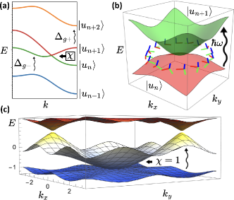
Figure 1: (a) Optical transitions to and from Euler bands with lower and upper gaps with energies $\Delta_{g-}$ and $\Delta_{g+}$. (b) Quadratic Euler node with non-trivial patch Euler class $\chi=1$ as captured by an effective ${\bf k}\cdot{\bf p}$ model. The associated eigenstate frame winding (colored vectors) corresponding to the winding of the non-Abelian connection $\textbf{A}_{1,2}$, which is singular at the node, and an optical transition within the Euler band subspace (for semimetallic doping) are shown schematically. (c) Lattice-regularized realization of the quadratic Euler node in a kagome model. The optical weights, as well as jerk conductivities, can be used to deduce the patch Euler class $\chi$.

Optical manifestations of Euler bands.— We first consider the case of Euler bands being fully isolated, and begin by discussing bounds on the optical observables captured by quantum geometric quantities, which can be used to infer the presence of a non-trivial Euler class in bands. As shown in Fig. 1(a), we label the magnitude of the (direct) gaps below and above the Euler bands $\{\ket{u_{n}},\ket{u_{n+1}}\}$ of energies $E_{n}({\bf k})$, $E_{n+1}({\bf k})$ as $\Delta_{g-}\equiv\text{min}_{\bf k}\left[E_{n}({\bf k})-E_{n-1}({\bf k})\right]$ and $\Delta_{g+}\equiv\text{min}_{\bf k}\left[E_{n+2}({\bf k})-E_{n+1}({\bf k})\right]$ respectively. Before deriving the bounds, we recall the inequality imposed on quantum geometry due to the non-triviality of the Euler class Ahn et al. (2021); Bouhon et al. (2023), as it forms the basis of further calculations. We define the quantum metric in the Euler bands as $g^{\chi}_{ab}({\bf k})=\mathfrak{Re}~{}\sum^{2}_{n=1}\sum_{m\neq 1,2}\left[r^{a}_{nm}r^{b}_{mn}\right]$, where $a,b=x,y$, and the ${r^{a}_{nm}=(1-\delta_{n,m})A^{a}_{n,m}}$ are transition dipole matrix elements captured by the components of the non-Abelian Berry connection $A^{a}_{n,m}$. The integral of the trace of $g^{\chi}_{ab}$ over the BZ can be shown to be bounded from below by the Euler class of the two-band subspace,

$$\frac{1}{4\pi}\int\differential^{2}{\bf k}~{}\Tr\textbf{g}^{\chi}\geq|\chi|,$$ (3)

where the trace is over ${\bf k}$-space coordinates at each ${\bf k}$-point individually (see Refs. Xie et al. (2020); Bouhon et al. (2023) and Appendix A). On the other hand, in three-band models, the Euler class is also captured by the winding of the third, fully-gapped, band vector $\textbf{n}_{3}\equiv\ket{u_{3}}$, and may be expressed as ${\chi=\frac{1}{4\pi}\int\differential^{2}{\bf k}~{}\textbf{n}_{3}\cdot(\partial_{k_{x}}\textbf{n}_{3}\crossproduct\partial_{k_{y}}\textbf{n}_{3})}$ Ünal et al. (2020). In this case, the LHS of Eq. (3) reduces to $\frac{1}{4\pi}\int\differential^{2}{\bf k}~{}\Tr\textbf{g}^{\chi}=\frac{1}{4\pi}\int\differential^{2}{\bf k}~{}{(|\partial_{k_{x}}\textbf{n}_{3}|^{2}+|\partial_{k_{y}}\textbf{n}_{3}|^{2})}$. In fact, this is the result of a stronger inequality that holds at every point in the BZ (i.e. between the integrands). Namely, ${|\partial_{k_{x}}\textbf{n}_{3}|^{2}+|\partial_{k_{y}}\textbf{n}_{3}|^{2}}\geq{|\textbf{n}_{3}\cdot(\partial_{k_{x}}\textbf{n}_{3}\crossproduct\partial_{k_{y}}\textbf{n}_{3})|}$, which is analogous to a similar geometric bound in Chern insulators, which arises from the skyrmion formula Piéchon et al. (2016); Onishi and Fu (2023). This inequality suggests a rich interplay between the Euler class and optical phenomena.

The quantum metric is also related to the intrinsic quadrupole moment of the bands, the quantity upon which electric quadrupole (E2) transitions depend Ahn et al. (2021); Ocaña and Souza (2023). In Euler phases, since the diagonal elements of the Berry connection vanish due to the reality condition, this culminates in the single-particle quadrupole moment given by ${q^{n}_{ab}({\bf k})\equiv-\frac{e}{2}\left(\bra{\partial_{k_{a}}u_{n}}\ket{\partial_{k_{b}}u_{n}}+\bra{\partial_{k_{a}}u_{n}}\ket{\partial_{k_{b}}u_{n}}\right)}$, where $e$ is the elementary charge. Consequently, by employing $q^{1}_{ab}+q^{2}_{ab}=-eg^{\chi}_{ab}$ for a real Hamiltonian, we find that Eq. (3) leads to a bound on the integrated total quadrupole moment of the topological bands due to their finite Euler class,

$$\frac{1}{4\pi}\int\differential^{2}{\bf k}~{}|\Tr(q^{1}_{ab}+q^{2}_{ab})|\geq e|\chi|.$$ (4)

In particular, we here consider coupling to an electric field ${\mathcal{E}=(\mathcal{E}_{x}\cos\omega t,\mathcal{E}_{y}\cos(\omega t+\phi))}$, where the phase shift $\phi$ controls the polarization, with $\phi=\pm\pi/2$ corresponding to left- and right-circularly polarized light (LCP/RCP). In this context, the quantum metric can be accessed by inspection of the appropriate optical weight $W^{1}_{ab}(\omega_{\text{max}})\equiv\int^{\omega_{\text{max}}}_{0}\differential\omega~{}\frac{\mathfrak{Re}~{}\sigma_{ab}(\omega)}{\omega}$, for the optical conductivities $\sigma_{ab}(\omega)$ under the electric field up to some large frequency $\omega_{\text{max}}$ (see Appendix B for further elaboration).

We now focus on the optical weights associated with transitions to and from the Euler subspace, which apply to arbitrarily dispersive Euler bands such as those naturally arising in lattice models (for concrete examples see Appendix F,  Bouhon and Slager (2022); Slager et al. (2022b); Jiang et al. (2021)). In this general context, as one of our central results, we derive an optical bound constraining the optical weights $W^{1}_{ab}$ involving the Euler bands, across the gaps harbouring $\Delta_{g-}$ and $\Delta_{g+}$, (see Fig. 1) Souza et al. (2000); Onishi and Fu (2023). More precisely, we label optical transitions into the isolated Euler subspace from bands below, and out of this subspace into bands above by unoccupied (unocc) and occupied (occ), respectively. We find that these transitions involving the Euler bands are indeed bounded by the multi-gap invariant,

$$\begin{split}&W^{1}_{xx,(\text{occ})}(\infty)+W^{1}_{yy,(\text{occ})}(\infty)\\ &+W^{1}_{xx,(\text{unocc})}(\infty)+W^{1}_{yy,(\text{unocc})}(\infty)\geq\frac{e^{2}}{\hbar}|\chi|,\end{split}$$ (5)

which holds in the high-frequency limit $\omega_{\text{max}}\rightarrow\infty$, as detailed in Appendix C. In particular, if there are no bands below the Euler subspace, then ${W^{1}_{aa,(\text{unocc})}(\infty)}$ vanishes, and the condition in Eq. (5) reduces to,

$$W^{1}_{xx,(\text{occ})}(\infty)+W^{1}_{yy,(\text{occ})}(\infty)\geq\frac{e^{2}}{\hbar}|\chi|,$$ (6)

which is observable for topological phases with $\chi\neq 0$. We numerically corroborate these results in models with different Euler class (see Fig. 2). Finally, we can also generalize these results to signatures of the quantum metric in flat-band systems with DC linear conductivity due to the interband contributions Mitscherling and Holder (2022), as detailed in Appendix D.

We remark that an analogous conclusion, viewed as a bound on the absorption captured by the optical weight, can be also reached directly from Fermi’s golden rule under circular polarization Ozawa and Goldman (2018). Namely, we find that the combined absorption rate $\tilde{\Gamma}^{\text{tot}}$ of LCP and RCP light Tran et al. (2017); Asteria et al. (2019), combining all possible transitions when Euler bands are fully occupied and when these are completely unoccupied, is bounded from below by the Euler class,

$$\tilde{\Gamma}^{\text{tot}}=\frac{2\pi\mathcal{E}^{2}}{\hbar}\int\differential^{2}{\bf k}~{}\Tr\textbf{g}^{\chi}~{}\geq\frac{\mathcal{E}^{2}}{2\hbar}|\chi|.$$ (7)

This result is indeed consistent with Eq. (5), on recognizing that combinations of LCP and RCP can be viewed as linear polarizations inducing corresponding excitations which appear in the definitions of the optical weights (see Appendix G for details).

We conclude by showing that the bound on the optical weight is additionally related to the size of the gaps in Euler phases. To prove this, we start by considering a three-band case with the Euler bands at the lowest energies, and apply the $f$-sum rule, as in Ref. Onishi and Fu (2023), to recognize that $\int^{\infty}_{0}\differential\omega~{}\frac{\mathfrak{Re}~{}\sigma^{aa}}{\omega}\leq\int^{\infty}_{0}\differential\omega~{}\mathfrak{Re}~{}\sigma^{aa}\frac{\hbar}{\Delta_{g}}=\frac{n_{e}\hbar e^{2}}{2m\Delta_{g}}$. As a result, we obtain that

$$\frac{n_{e}\pi\hbar^{2}}{m\Delta_{g}}\geq|\chi|\implies\frac{n_{e}\pi\hbar^{2}}{m|\chi|}\geq\Delta_{g},$$ (8)

where $n_{e}$ is the charge density in the occupied bands, $\Delta_{g}$ is the band gap, and $m$ is the bare electron mass. A tighter bound can be obtained on replacing the bare mass $m$ (from the minimal coupling Hamiltonian) with the effective mass $m^{*}$ in the $f$-sum rule (within the ${\bf k}\cdot{\bf p}$ approach) Onishi and Fu (2023). In the flat band limit, a non-zero Euler class $|\chi|\neq 0$ implies that the gap $\Delta_{g}$ must vanish in the limit of large effective mass $m^{*}\rightarrow\infty$. Hence, to keep the gap finite, an Euler insulator necessarily needs dispersion in either the Euler bands or the unoccupied band above the gap, by symmetry with respect to the optical transitions on inverting the band structure. In the generalized many-band case (with more bands), we analogously employ the sum rule to obtain,

$$\frac{\pi\hbar^{2}}{m}\left(\frac{n_{e,\text{occ}}}{\Delta_{g-}}+\frac{n_{e,\text{unocc}}}{\Delta_{g+}}\right)\geq|\chi|,$$ (9)

where $n_{e,\text{occ}},n_{e,\text{unocc}}\sim 1/a^{2}$ (with $a$ the lattice constant) are the total charge densities for the cases where the Euler bands are occupied and unoccupied respectively as before. In fact, an even stricter bound can be obtained by demanding that $n_{e,\text{unocc}}$ is the carrier density, as found in certain ${\bf k}\cdot{\bf p}$ low-energy formulations of twisted bilayer graphere models Tarnopolsky et al. (2019); Bernevig et al. (2021); Bennett et al. (2023). Therefore, the Euler class of the bands constrains the size of both gaps as

$$\frac{n_{e,\text{unocc}}\pi\hbar^{2}}{m|\chi|}\geq\frac{n_{e,\text{unocc}}}{\frac{n_{e,\text{occ}}}{\Delta_{g-}}+\frac{n_{e,\text{unocc}}}{\Delta_{g+}}}\geq\frac{1}{2}\text{HM}(\Delta_{g-},\Delta_{g+}),$$ (10)

where $\text{HM}(\Delta_{g-},\Delta_{g+})\equiv[(\Delta_{g+}^{-1}+\Delta_{g-}^{-1})/2]^{-1}$ is the harmonic mean of the band gaps, and we have used $n_{e,\text{occ}}\geq n_{e,\text{unocc}}$. This is the central result of this work, elucidating a quantum-geometric constraint on the multi-gap Euler topology in electronic materials, as manifested by a fundamental optical bound on the band gaps. Contrary to the bounds related to DC conductivity within non-interacting particle picture (see Appendix D), this kind of fundamental bound should hold even in interacting, strongly correlated systems Onishi and Fu (2023).

Optical manifestations of patch Euler class.— We now demonstrate how our findings generalize for a patch Euler invariant, which extend beyond Euler subspaces fully separated by gaps $\Delta_{g\pm}$ (see Fig. 1). A patch of two bands with $\chi\neq 0$ necessarily hosts band nodes with the same non-Abelian frame charges that are obstructed to annihilate each other  Bouhon et al. (2020c), as long as the patch excludes band crossings of other bands Bouhon et al. (2020b). However, accessing this Euler invariant and non-Abelian properties can be complicated due to the multi-band character of Euler class Bouhon et al. (2020c). We here show that the invariant can be probed with AC conductivities, associated optical weights, and third-order jerk photoconductivities Fregoso et al. (2018).

A general $\textbf{{\bf k}}\cdot{\bf p}$ Hamiltonian for a bulk Euler node hosting a patch Euler class can be written as

$$H_{\chi}({\bf k})=\alpha(k_{+}^{2|\chi|}\sigma_{-}+k^{2|\chi|}_{-}\sigma_{+}),$$ (11)

where $\alpha$ is a dispersion constant, $k_{\pm}=k_{x}\pm\mathrm{i}k_{y}$ and ${\sigma_{\pm}=(\sigma_{x}\pm\mathrm{i}\sigma_{z})/2}$ Morris et al. (2023). Note that the the Hamiltonian is real by construction. The elements of the non-Abelian Berry connection, the quantum metric, and associated optical responses, may be directly computed from the eigenstates of $H_{\chi}({\bf k})$. We find that on doping the chemical potential $\mu$ away from the node (cf. Appendix E), the optical weight is given by

$$W^{1}_{xx}(\omega_{\text{max}})=\frac{\pi^{3}e^{2}}{h}|\chi|\text{ln}\left(\frac{\omega_{\text{max}}}{2\mu}\right).$$ (12)

Hence, since $\omega_{\text{max}}$ and $\mu$ are controllable parameters, we find that the patch Euler class can be indeed deduced by measuring the AC conductivity of an Euler semimetal subject to doping.

As a next step, we also demonstrate that independently of the dispersion proportionality constant $\alpha$, the jerk conductivities Fregoso et al. (2018) at any non-vanishing light frequency $\omega$ offer universal Euler class-dependent ratios, see Appendix E for the derivations. Most interestingly, we obtain that

$$\frac{\sigma^{xxxx}_{\text{jerk}}(\omega)}{\sigma^{xxyy}_{\text{jerk}}(\omega)}=\frac{3|\chi|-1}{|\chi|+1},$$ (13)

which is always non-vanishing and bounded: ${1<\sigma^{xxxx}_{\text{jerk}}/\sigma^{xxyy}_{\text{jerk}}<3}$. This holds provided that, at least to a first order, the node (i) is rotationally-symmetric, and (ii) hosts a patch Euler class $\chi$. We also note that the nature of the low-frequency divergence of jerk photoconductivities $\omega\rightarrow 0$ depends on $\chi$, becoming weaker as $\chi$ increases. As shown in Appendix E, all second-order photoconductivities vanish within the model, as the bulk node naturally enjoys the inversion symmetry. When full rotational symmetry is not globally preserved, as in lattice models, we find that Eqs. (12) and (13) hold in the close proximity of the node.

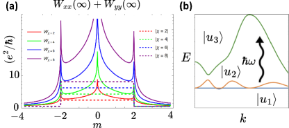
Figure 2: (a) Optical weights in a three-band Euler Hamiltonian with the occupied Euler bands (lowest two bands as depicted in (b)) can be related to the interband contribution to the linear DC conductivities. The combined optical weight is bounded by the Euler invariant as given by Eq. (6). Singularities occur at topological phase transitions ($|m|=2$), associated with the closing of the gap between the two-band Euler subspace and a trivial band as the topological mass term $m$ is changed. The limit of large $|m|$ corresponds to the trivial phase with $\chi=0$. (b) A schematic picture of the corresponding transitions.

Reconstructing the Euler invariant.— Finally, we demonstrate that the multi-gap Euler invariant (1) can be probed directly by monitoring the transition rates in a frequency- and momentum-resolved way. Motivated by the reconstruction of the full quantum geometric tensor (QGT) Ozawa and Goldman (2018); Gianfrate et al. (2020), we device a protocol by considering only the bottom band of the Euler subspace occupied (not both), see Fig. 1(b). We recognize that both terms of Eq. (1) can be extracted from the elements of the non-Abelian Berry connection, which we identify in the real part of the QGT. Specifically, the vector components of the non-Abelian connection can be deduced from the absorption rate of the linearly-polarized light in the $x$-direction, probing $g^{12}_{xx}=|A^{x}_{12}|^{2}$, and the $y$-direction, probing $g^{12}_{yy}=|A^{y}_{12}|^{2}$. The non-Abelian connection vector can be thus obtained modulo the sign of each component, where we impose a smooth real gauge by hand to fix the sign as a gauge choice. This allows to compute the Euler curvature and the Euler invariant.

Numerical verification in representative models.— Given the general formulation of Euler models using Plücker embeddings Bouhon et al. (2020a); Bouhon and Slager (2022) we can readily corroborate our results in the context of concrete, lattice-regularized, tight-binding models. To this end, we consider illustrative three-band and four-band models on square and kagome lattices, which can be also adapted experimentally in trapped-ion simulators and metamaterials Ünal et al. (2020); Jiang et al. (2021, 2022). We present our numerical findings for optical weights in Fig. 2, demonstrating how the optical bounds from Eq. (5) are satisfied in topological phases (for further details, see Appendix D). Furthermore, in Fig. 3 we show how the Euler invariant can be numerically reconstructed from the optical transitions, as proposed in the previous section. Finally, we find that the result discovered from the ${\bf k}\cdot{\bf p}$ model of an Euler node transfer to the lattice-regularized realizations of Euler semimetals, see also Appendix F.

Discussion.— We will now further comment on the scope and applicability of our results. As derived analytically and verified numerically, our bounds on optical responses offer a route to probe many-band topology in simple Euler Hamiltonians within the independent-particle picture. We note that these models may be already implemented in trapped-ion simulators and metamaterial realizations. Additionally, the bounds on optical weights can be clearly understood microscopically in terms of the application of Fermi’s golden rule to interband transitions. In the case of nodal Euler topology, the relation between the optical weight and doping of an Euler semimetal naturally arises and is sensitive to the value of the patch Euler class. Here, the jerk conductivities, and other third-order effects, might provide a valuable insight, especially by means of low-frequency divergences Ahn et al. (2020). Even in the case of nodes being rotationally not symmetric, the ratios of photoconductivities obtained within the effective model may be modified. Additionally, on breaking the inversion symmetry assumed in the continuum model, linear injection, as well as circular shift photoconductivities (Appendix B, Appendix E) might arise, offering further insights into the physics induced by the non-Abelian connection constrained by the Euler invariant. Finally, the consequences of the derived bound on the gaps below and above the Euler bands can be contrasted with the effective models for twisted layered graphene systems Tarnopolsky et al. (2019); Bernevig et al. (2021) assuming flat bands with $\chi=1$, as well as with the single-gap Chern bounds in moiré MoTe₂ and WTe₂ Onishi and Fu (2023).

Conclusions and Outlook.— We demonstrated how the topological Euler class characterizing non-Abelian multi-gap topology can be optically probed in electronic systems. In particular, it can be exactly reconstructed from the optical absorption/excitation experiments. We showed using a quantum geometric bound that the presence of the two-band subspace hosting an Euler invariant enforces a lower bound on the optical weights and associated interband contributions to DC conductivities. Furthermore, we derived a fundamental bound constraining a harmonic mean involving both gaps neighboring the Euler bands. Lastly, we showed that Euler class in the non-degenerate band limit of an underdoped semimetal can also be related to optical weights and photoconductivities.

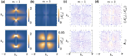
Figure 3: Mapping the Euler invariant. The absolute values of the components of the non-Abelian connection are constructed from the associated quantum metric probed by optical transition rates under linearly-polarized light. (a,b) We map out $|A^{x}_{12}|$ (upper panel) and $|A^{y}_{12}|$ (lower panel) for the Euler Hamiltonian with $\chi=2$ on square lattice, in the topological ($m=1$) (a) and trivial phase ($m=3$) (b). Correspondingly, the non-Abelian connection vectors can be reconstructed by fixing the signs of these components in a maximally smooth gauge, in (c) topological and (d) trivial phase.

Appendix A A brief introduction to quantum geometry

A.1 Bounds on multi-band invariants

In the following we briefly review elements of the non-Abelian quantum geometry of multi-band systems. To do so we will make use of the recently-established Plücker formalism, which allows for a concrete analysis of quantum geometry beyond the projective single-band description Bouhon et al. (2023). We further utilize this tool to describe the geometric quantities present in optical response in terms of Riemannian metrics; in a similar spirit to Refs. Ahn et al. (2020, 2021).

We define the non-Abelian quantum geometric tensor componentwise as Bouhon et al. (2023)

$$(\tilde{Q}_{ab})_{nm}=\bra{\partial_{a}u_{n,{\bf k}}}\hat{Q}_{l,{\bf k}}\ket{\partial_{b}u_{m,{\bf k}}}=\bra{\partial_{a}u_{n,{\bf k}}}1-\hat{P}_{l,{\bf k}}\ket{\partial_{b}u_{m,{\bf k}}},$$ (14a)

where $$\hat{P}_{l,{\bf k}}=\sum_{\ell\in l}\ket{u_{\ell,{\bf k}}}\bra{u_{\ell,{\bf k}}} l\subset\{1,\ldots,N\} a,b=k_{x},k_{y} n,m\in l$$ is the projector onto the manifold spanned by a subset of selected bands of interest Xie et al. (2020); Bouhon et al. (2023), which need not contain the entire manifold of occupied states. Here, as in the main text, the indices label momenta, while run over the chosen bands. The non-Abelian quantum metric corresponds to the real part of this tensor,

$$(\tilde{g}_{ab})_{nm}=\mathfrak{Re}~{}(\tilde{Q}_{ab})_{nm}=\mathfrak{Re}~{}\bra{\partial_{a}u_{n,{\bf k}}}\hat{Q}_{l,{\bf k}}\ket{\partial_{b}u_{m,{\bf k}}},$$ (14b)

while the non-Abelian Berry curvature is ($$-2$$ times) the imaginary part, that is

$$\mathcal{F}^{nm}_{ab}=-2\mathfrak{Im}~{}(\tilde{Q}_{ab})_{nm}=-2\mathfrak{Im}~{}\bra{\partial_{a}u_{n,{\bf k}}}\hat{Q}_{l,{\bf k}}\ket{\partial_{b}u_{m,{\bf k}}}.$$ (14c)

Eqs. (14) may be written in the combined form,

$$(\tilde{Q}_{ab})_{nm}=(\tilde{g}_{ab})_{nm}-\frac{\mathrm{i}}{2}\mathcal{F}^{nm}_{ab}\;.$$ (15)

Importantly, $\tilde{Q}_{ab}$ is positive semidefinite, $\bra{\psi}\hat{Q}\ket{\psi}\geq 0$, as is the non-Abelian quantum metric $\tilde{g}_{ab}$ Xie et al. (2020); Bouhon et al. (2023).

For any choice of bands $l$, one may define an Abelian quantum metric $g_{ab}$ by taking the trace of $\tilde{g}_{ab}$ over these chosen bands:

$$g_{ab}=\Tr_{l}\tilde{g}_{ab}\equiv\sum_{\ell\in l}\bra{u_{\ell}}\tilde{g}_{ab}\ket{u_{\ell}}.$$ (16)

In particular, by taking $l=l_{\text{occ}}$ to consist of all occupied bands, one obtains the Abelian quantum metric which is most commonly found in the literature, namely $g^{\text{occ}}_{ab}\equiv g^{l_{\text{occ}}}_{ab}\equiv\Tr\tilde{g}^{l_{\text{occ}}}_{ab}$. For an arbitrary subset $l$ of bands it can be seen that $g^{l}_{ab}=\Tr\tilde{g}^{l}_{ab}$ is also a Fubini-Study metric, and may be used to assign a ‘distance’ between the infinitesimally separated points ${\bf k}$ and ${\bf k}+\differential{\bf k}$ as Torma et al. (2018); Xie et al. (2020); Bouhon et al. (2023)

$$D^{2}({\bf k},{\bf k}+\differential{\bf k})=\frac{1}{2}\Tr\left[\left(P_{l,{\bf k}+\differential{\bf k}}-P_{l,{\bf k}}\right)^{2}\right]=g^{l}_{ab}({\bf k})\,dk_{a}\,dk_{b}.$$ (17)

We now turn to the relation of the non-Abelian quantum geometric tensor to multi-band topological invariants. To investigate the Euler topology of a subspace spanned by two bands $\ket{1}\equiv\ket{u^{1}_{\bf k}}$ and $\ket{2}\equiv\ket{u^{2}_{\bf k}}$ we set $l=\{1,2\}$ to consist of these bands only. In this case it can be seen that the Euler curvature, $\text{Eu}=-\mathrm{i}\mathcal{F}^{12}_{xy}$, appears directly within the quantum geometric tensor. The positive semidefiniteness of the geometric tensor in fact leads to the condition Eq. (3) on the Euler class that is used in the main text; we will now derive this equation. Using the shorthand ${\ket{\ell,a}\equiv\ket{\partial_{a}u^{\ell}_{\bf k}}}$, where $\ell\in l$, we may write

$$(\tilde{g}_{ab})_{nm}=\bra{n,a}\hat{Q}_{l,{\bf k}}\ket{m,b}$$ (18a)

and

$$\text{Eu}=\bra{1,y}\hat{Q}_{l,{\bf k}}\ket{2,x}-\bra{1,x}\hat{Q}_{l,{\bf k}}\ket{2,y}.$$ (18b)

Applying the quantum geometric tensor to a judiciously chosen set of states $\ket{\phi_{1}^{\pm}}=\frac{1}{\sqrt{2}}(\ket{1,y}\pm\ket{2,x})$ and $\ket{\phi_{2}^{\pm}}=\frac{1}{\sqrt{2}}(\ket{1,x}\pm\ket{2,y})$ then leads to a set of relations

$$\bra{\phi^{\pm}_{i}}\hat{Q}_{l,{\bf k}}\ket{\phi^{\pm}_{i}}\geq 0,\qquad i=1,2$$ (19)

which, by using the relation $\bra{n,i}\ket{m,j}=\bra{m,j}\ket{n,i}$ from the reality condition, may be rearranged to yield

$$\Tr\textbf{g}^{\chi}\equiv(\tilde{g}_{xx})_{11}+(\tilde{g}_{yy})_{11}+(\tilde{g}_{xx})_{22}+(\tilde{g}_{yy})_{22}\geq\pm 2\text{Eu},$$ (20)

or, more compactly, $\Tr\textbf{g}^{\chi}\geq 2|\text{Eu}|$. Hence, upon performing the integration over the BZ we arrive at the required inequality

$$\frac{1}{4\pi}\int_{\text{BZ}}\differential^{2}{\bf k}~{}\Tr\textbf{g}^{\chi}\geq\left|\frac{1}{2\pi}\int_{\text{BZ}}\differential^{2}{\bf k}~{}\mathrm{Eu}\right|=|\chi|,$$ (21)

which is central to the main text.

A.2 Riemannian geometry of Bloch states

In the context of optical responses relevant to this work, we identify the transition dipole moment ${\bf r}_{mn}({\bf k})=\bra{\psi_{m{\bf k}}}\hat{{\bf r}}\ket{\psi_{n{\bf k}}}$ as a tangent vector on the manifold of quantum states Ahn et al. (2021), with components

$${\bf r}^{a}_{mn}({\bf k})=\mathrm{i}\delta_{mn}\partial_{a}-A^{a}_{n,m}({\bf k})\;,$$ (22)

where $A^{a}_{n,m}({\bf k})\equiv\bra{u_{n,{\bf k}}}\ket{\partial_{a}u_{m,{\bf k}}}$ is the non-Abelian Berry connection, and $\partial_{a}\equiv\frac{\partial}{\partial_{k_{a}}}$ is a tangent vector component induced by the local coordinates $\{k_{a}\}$. The manifold upon which these objects are defined depends upon the physical context. For example, if no degeneracies are present then the manifold of states for an $N$-band system is a complex flag manifold $\widetilde{\mathsf{Fl}}_{1,1,\ldots,1}(\mathbb{C})=U(N)/U(1)^{N}$, where the quotient is due to the gauge freedom in each band. In the case of Euler phases, or more general multi-gap topology under the symmetry-enforced reality conditions, central to this work, the manifold of interest, accounting for band degeneracies, extends to: $\widetilde{\mathsf{Fl}}_{p_{1},\ldots,p_{k}}(\mathbb{R})=O(N)/(O(p_{1})\crossproduct\ldots\crossproduct O(p_{k})$, where the number of bands in isolated subspaces $k$ sums to $N=p_{1}+\ldots+p_{k}$.

Following Ref. Ahn et al. (2021), we define a Hilbert-Schmidt inner product of matrices as,

$$\langle A,B\rangle=\Tr\left[A^{\dagger}B\right]=\sum_{a,b}A^{*}_{ab}B_{ab}\;,$$ (23)

which allows the Abelian quantum geometric tensor to be represented in terms of the local interband transition vectors $\hat{e}^{mn}_{a}({\bf k})={\bf r}^{a}_{mn}({\bf k})\ket{u_{m,{\bf k}}}\bra{u_{n,{\bf k}}}$ as

$$Q^{mn}_{ab}\equiv\langle\hat{e}^{mn}_{a},\hat{e}^{nm}_{b}\rangle=r^{a}_{nm}r^{b}_{mn}.$$ (24)

The advantage of this representation is that it allows us to easily introduce a Hermitian connection as

$$C^{mn}_{acb}\equiv\langle\hat{e}^{mn}_{a},\nabla_{c}\hat{e}^{nm}_{b}\rangle=r^{a}_{nm}r^{b;c}_{mn}=\sum_{d}Q^{mn}_{ad}(C^{mn})^{d}_{cb}$$ (25)

where the covariant derivative acts on the transition vectors as $\nabla_{c}\hat{e}^{mn}_{a}=\sum_{b}(C^{mn})^{b}_{ca}\hat{e}^{mn}_{b}$. The covariant derivative $r^{b;c}_{nm}$ of the transition dipole is defined in terms of the the (Abelian part of the) Berry connection as

$$\begin{split}r^{c;a}_{nm}({\bf k})=\nabla_{a}r^{c}_{nm}({\bf k})=\partial_{a}r^{c}_{nm}({\bf k})-\mathrm{i}(A^{a}_{nn}({\bf k})-A^{a}_{mm}({\bf k}))r^{c}_{nm}({\bf k}).\end{split}$$ (26)

Correspondingly, the Christoffel symbols for the metric connection are given by

$$\Gamma^{mn}_{abc}=\frac{1}{2}(\partial_{c}g^{mn}_{ba}+\partial_{b}g^{mn}_{ca}-\partial_{c}g^{mn}_{ab})=\mathfrak{Re}~{}\left[r^{a}_{nm}r^{b;c}_{mn}\right],$$ (27)

while the torsion tensor is defined as $T^{mn}_{acb}=C^{mn}_{acb}-C^{mn}_{abc}$, and the symplectic connection can be defined as ${\tilde{\Gamma}_{acb}=\mathrm{i}(C_{acb}-C^{*}_{acb})}$. Finally, we define the Hermitian curvature tensor as

$$\begin{split}K^{mn}_{abcd}\equiv\left\langle\hat{e}^{mn}_{a},(\nabla_{d}\nabla_{c}-\nabla_{c}\nabla_{d})\hat{e}^{nm}_{b}\right\rangle=\sum_{d}Q^{mn}_{ae}(C^{mn})^{d}_{cb},\end{split}$$ (28)

and moreover we define the Riemannian curvature tensor as the real part of this object, that is, $R^{mn}_{cbad}=\mathfrak{Re}~{}\{K^{mn}_{cbad}\}$. This completes our glossary of quantum Riemannian objects relevant to this work.

Appendix B Optical responses and quantum geometry

The geometric quantities introduced in the previous section are physically related to the experimentally accessible (AC) optical conductivity

$$\sigma^{ab}=\frac{\pi\omega e^{2}}{\hbar}\sum_{m,n}\int\frac{\differential^{d}k}{(2\pi)^{d}}\delta(\omega-\omega_{mn})f_{nm}Q^{mn}_{ab},$$ (29)

where, ${\omega=\omega_{mn}=\frac{1}{\hbar}(E_{m,{\bf k}}-E_{n,{\bf k}})}$ is the resonant frequency for transition, and $f_{mn}=f_{n{\bf k}}-f_{m{\bf k}}$ is the difference in Fermi-Dirac occupation factors. More directly, the interband contribution to the imaginary part of the dielectric tensor, which encodes optical absorption, explicitly contains the quantum metric:

$$\epsilon^{\prime\prime}_{ab}(\omega)=\frac{\pi e^{2}}{\hbar}\sum_{m,n}\int\frac{\differential^{d}k}{(2\pi)^{d}}\delta(\omega-\omega_{mn})f_{nm}g^{mn}_{ab}\;.$$ (30)

Higher-order optical responses contain a plethora of quantum geometric quantities Ahn et al. (2021): the second-order shift photoconductivity is

$$\sigma^{cab}_{\text{shift}}=-\frac{\pi e^{3}}{2\hbar^{2}}\sum_{m,n}\int\frac{\differential^{d}k}{(2\pi)^{d}}\delta(\omega-\omega_{mn})f_{nm}\mathrm{i}\left(C^{mn}_{acb}-(C^{mn}_{bca})^{*}\right),$$ (31a)

and the second-order injection photoconductivity is

$$\sigma^{cab}_{\text{inj}}=-\frac{\pi e^{3}\tau}{\hbar^{2}}\sum_{m,n}\int\frac{\differential^{d}k}{(2\pi)^{d}}\delta(\omega-\omega_{mn})f_{nm}Q^{mn}_{ab}\partial_{c}\omega_{mn},$$ (31b)

where $$\tau$$ is the relaxation time for the photo-excited particle to decay; furthermore, the third-order jerk photoconductivity is given by

$$\sigma^{cdab}_{\text{inj}}=-\frac{2\pi e^{4}\tau}{\hbar^{3}}\sum_{m,n}\int\frac{\differential^{d}k}{(2\pi)^{d}}\delta(\omega-\omega_{mn})f_{nm}Q^{mn}_{ab}\partial_{c}\partial_{d}\omega_{mn}.$$ (31c)

One may also define a third-order injection photoconductivity, which depends on $K^{mn}_{cbad}$ Ahn et al. (2021), as well as a third-order shift photoconductivity Fregoso (2019). Note that the second-order shift conductivity does not require any dispersion in the band structure, contrary to the injection and jerk conductivities. These correspondingly depend on the group velocity matrix elements (${v^{c}_{mm}-v^{c}_{nn}=\partial_{c}\omega_{mn}}$) and effective masses (${(m^{-1}_{*})_{cd,m}-(m^{-1}_{*})_{cd,n}=\frac{1}{\hbar}\partial_{c}\partial_{d}\omega_{mn}}$) in bands $m,n$ between which the photo-excitation occurs.

The optical conductivity can be decomposed as

$$\sigma^{ab}(\omega)=\mathfrak{Re}~{}\sigma^{ab}(\omega)+\mathrm{i}\mathfrak{Im}~{}~{}\sigma^{ab}(\omega),$$ (32)

and we define generalized optical weights Onishi and Fu (2023) as

$$W^{\kappa}_{ab}(\omega_{\text{max}})=\int_{0}^{\omega_{\text{max}}}\differential\omega~{}\frac{\mathfrak{Re}~{}\sigma^{ab}(\omega)}{\omega^{\kappa}}.$$ (33)

In particular, for $\kappa=1$,

$$\begin{split}W^{1}_{ab}(\omega_{\text{max}})=\int_{0}^{\omega_{\text{max}}}\differential\omega~{}\frac{\mathfrak{Re}~{}\,\sigma^{ab}(\omega)}{\omega}=\frac{\pi e^{2}}{\hbar}\sum_{m,n}\int\frac{\differential^{d}k}{(2\pi)^{d}}\theta(\omega_{\text{max}}-\omega_{mn})f_{nm}g^{mn}_{ab},\end{split}$$ (34)

where $\theta(\omega_{\text{max}}-\omega_{mn})$ is the Heaviside step function, which acts to select contributions up to a maximum frequency $\omega_{\text{max}}$. Using the Kramers-Kronig relations

$$\frac{2}{\pi}P\int_{0}^{\infty}\differential\omega~{}\frac{\mathfrak{Re}~{}\sigma^{ab}(\omega)}{\omega-\omega^{\prime}}={} \mathfrak{Im}~{}\sigma^{ab}(\omega^{\prime}),$$ (35a)

$$-\frac{2}{\pi}P\int_{0}^{\infty}\differential\omega~{}\frac{\mathfrak{Im}~{}\sigma^{ab}(\omega)}{\omega-\omega^{\prime}}={} \mathfrak{Re}~{}\sigma^{ab}(\omega^{\prime}),$$ (35b)

along with the identity $\sigma^{ab}(\omega)=\sigma^{ab}(-\omega)^{*}$, and setting $\omega^{\prime}=0$, we observe that

$$\mathfrak{Im}~{}\sigma^{ab}(0)=\frac{2e^{2}}{\hbar}\sum_{m,n}\int\frac{\differential^{d}k}{(2\pi)^{d}}f_{nm}g^{mn}_{ab}=\sigma_{\text{inter}}^{ab}(0),$$ (36)

Where we have identified $\sigma_{\text{inter}}^{ab}(0)$, the quantum interband contribution to the DC longitudal conductivity Mitscherling (2020); Mitscherling and Holder (2022). Similarly, the real part of the DC conductivity is

$$\mathfrak{Re}~{}\sigma^{ab}(0)=-\frac{2e^{2}}{\hbar}\sum_{m,n}\int\frac{\differential^{d}k}{(2\pi)^{d}}f_{nm}\left(-\frac{F^{mn}_{ab}}{2}\right).$$ (37)

This identity contains as a special case the famous TKNN formula Thouless et al. (1982)

$$\begin{split}\sigma_{xy}=\mathfrak{Re}~{}\sigma^{xy}(0)=\frac{e^{2}}{\hbar}\sum_{m,n}\int\frac{\differential^{2}k}{(2\pi)^{2}}f_{nm}F^{mn}_{xy}=\frac{e^{2}}{2\pi\hbar}\sum_{n}\frac{1}{2\pi}\int\differential^{2}k~{}F^{nn}_{xy}=\frac{e^{2}}{h}\sum_{n}C_{n}.\end{split}$$ (38)

which describes the quantization of the (anomalous) Hall conductivity, $\sigma_{xy}$, in two-dimensions. We therefore see that while the second Kramers-Kronig relation Eq. 35b provides information about the Chern topology, it is the other Kramers-Kronig relation Eq. 35a that is central to indicating the presence of Euler topology, as explained in the main text.

Similarly to the first-order optical conductivity, both the injection and shift conductivities can be decomposed in terms of linear ($L$) and circular ($C$) terms (probed by linearly/circularly polarized light, respectively) as

$$\sigma^{cab}_{\text{inj}}=\sigma^{cab}_{\text{inj},L}+\mathrm{i}\sigma^{cab}_{\text{inj},C}.$$ (39)

For instance, the bulk linear shift photoconductivity for a two-dimensional system is given by Ibanez-Azpiroz et al. (2018):

$$\begin{split}\sigma^{cab}_{\text{shift},L}(\omega)=\frac{\pi e^{3}}{2\hbar^{2}}\int\frac{\differential^{2}k}{(2\pi)^{2}}\sum_{nm}(f_{n{\bf k}}-f_{m{\bf k}})\mathfrak{Im}~{}\big{[}r^{b}_{nm}({\bf k})r^{c;a}_{mn}({\bf k})+r^{b}_{nm}({\bf k})r^{ca}_{mn}({\bf k})\big{]}\delta(\omega_{mn}-\omega).\end{split}$$ (40)

It is immediately clear that, under the reality condition required for non-trivial Euler topology, the integral vanishes, and $\sigma^{cab}_{\text{shift},L}(\omega)=0$. Similarly, the vanishing of the Abelian Berry curvature, which follows from the vanishing of the Abelian connection in Euler materials, necessarily implies $\sigma^{cab}_{\text{inj},C}(\omega)=0$.

The photoconductivities defined above describe the DC responses induced by an applied electric field; such responses are of general interest in the context of photovoltaic applications Cook et al. (2017); Alexandradinata (2022). We briefly mention a few cases of particular importance: firstly

$$j^{c}_{\text{shift/inj}}(0)=2\sum_{a,b}\sigma^{cab}_{\text{shift/inj}}(\omega)\mathcal{E}^{a}(\omega)\mathcal{E}^{b}(-\omega),$$ (41a)

for second order DC currents; at third-order we have

$$j^{d}_{\text{shift/inj}}(0)={} 6\sum_{a,b,c}\sigma^{dabc}_{\text{shift/inj}}(\omega)\mathcal{E}^{a}(\omega)\mathcal{E}^{b}(-\omega)\mathcal{E}^{c}(0)$$ (41b)

$$j^{d}_{\text{jerk}}(0)={} 6\sum_{a,b,c}\sigma^{dcab}_{\text{jerk}}(\omega)\mathcal{E}^{a}(\omega)\mathcal{E}^{b}(-\omega)\mathcal{E}^{c}(0)$$ (41c)

where $E^{d}(0)$ is an additional DC electric field component. Importantly, different photoconductivities can be probed with both linearly and circularly polarized light, inducing corresponding dynamical responses.

Finally, as shown in Ref. Ahn et al. (2021), we note that there also exists a manifestation of the last geometric quantity introduced in the previous section, namely the Riemann curvature tensor $R^{mn}_{cbad}$,

$$\chi_{m,n}=C_{m}-C_{n}=\frac{1}{2\pi}\oint_{\text{BZ}}\differential^{2}k\frac{\text{sgn}(-\mathfrak{Im}~{}Q^{mn}_{12})R^{mn}_{1212}}{\sqrt{\text{det}(g^{mn})}}\;,$$ (42)

in a topological optical photovoltaic Hall response. This response is captured by so-called ‘Euler numbers’ $\chi_{m,n}$ defined as differences of Chern numbers of bands $m$ and $n$, correspondingly $C_{m}$ and $C_{m}$. Importantly, as can be checked by inspection, these Euler numbers are distinct from the Euler class $\chi$ of two neighboring bands with band crossings, which can be viewed as the Chern number of the complexification of two bands: $\chi(\ket{u_{n}},\ket{u_{n+1}})=C\big{[}\frac{1}{\sqrt{2}}(\ket{u_{n}}+\mathrm{i}\ket{u_{n+1}})\big{]}$, rather than as the difference of their Chern numbers.

Appendix C Derivation of the bound on the combined optical weights in Euler materials

In this Appendix we derive the bound, Eq. 5, on the combined optical weights at zero temperature due to the non-trivial Euler class.

We consider a system with a total of $N$ bands (in particular a limit of infinitely, but countably many bands $N\rightarrow\infty$ can be taken), where the bands $M+1$ and $M+2$ (with $M+2\leq N$) together form a non-trivial Euler subspace. With reference to Eq. 16, we define three distinct quantum metrics in this space by specifying the bands $l$ with which they are associated. Firstly, we define the metric of the Euler bands only as $g^{\chi}\equiv g^{l_{\chi}}$, where $l_{\chi}=\{M+1,M+2\}$. Secondly, we suppose that the chemical potential of the system sits between the bands $M+2$ and $M+3$, so that the Euler bands are occupied, and define $g_{\text{occ}}\equiv g^{l_{\text{occ}}}$, with $l_{\text{occ}}=\{1,\ldots,M,M+1,M+2\}$. Finally, we define a metric for the case that the chemical potential sits between bands $M$ and $M+1$, so that the Euler subspace is unoccupied, and $g_{\text{unocc}}\equiv g^{l_{\text{unocc}}}$ with $l_{\text{unocc}}=\{1,\ldots,M\}$. For later convenience we also let $l_{0}=\{1,\ldots,N\}$ and define $\bar{l}_{\text{occ}}=l_{0}\backslash l_{\text{occ}}=\{M+3,\ldots,N\}$, $\bar{l}_{\text{unocc}}=l_{0}\backslash l_{\text{unocc}}=\{M+1,\ldots,N\}$, and $\bar{l}_{\chi}=l_{0}\backslash l_{\chi}=\{1,\ldots,M,M+3,\ldots,N\}$. Note that $\bar{l}_{\chi}=l_{\text{unocc}}\cup\bar{l}_{\text{occ}}$, $l_{\text{occ}}=l_{\chi}\cup l_{\text{unoc}}$, and $\bar{l}_{\text{unocc}}=l_{\chi}\cup\bar{l}_{\text{occ}}$. Using the definition Eq. 14, we may then write each of these metrics in terms of the Berry connection as follows:

$$[g_{\chi}]_{aa}={} \sum_{n\in l_{\chi}}\sum_{m\in\bar{l}_{\chi}}|A^{a}_{nm}|^{2}=\sum_{n\in l_{\chi}}\sum_{m\in\bar{l}_{\text{occ}}}|A^{a}_{nm}|^{2}+\sum_{n\in l_{\chi}}\sum_{m\in l_{\text{unocc}}}|A^{a}_{nm}|^{2}\equiv X_{1}+X_{2},$$ (43a)

$$[g_{\text{occ}}]_{aa}={} \sum_{n\in l_{\text{occ}}}\sum_{m\in\bar{l}_{\text{occ}}}|A^{a}_{nm}|^{2}=\sum_{n\in l_{\chi}}\sum_{m\in\bar{l}_{\text{occ}}}|A^{a}_{nm}|^{2}+\sum_{n\in l_{\text{unocc}}}\sum_{m\in\bar{l}_{\text{occ}}}|A^{a}_{nm}|^{2}\equiv O_{1}+O_{2},$$ (43b)

$$[g_{\text{unocc}}]_{aa}={} \sum_{n\in l_{\text{unocc}}}\sum_{m\in\bar{l}_{\text{unocc}}}|A^{a}_{nm}|^{2}=\sum_{n\in l_{\text{unocc}}}\sum_{m\in l_{\chi}}|A^{a}_{nm}|^{2}+\sum_{n\in l_{\text{unocc}}}\sum_{m\in\bar{l}_{\text{occ}}}|A^{a}_{nm}|^{2}\equiv U_{1}+U_{2}.$$ (43c)

It can be immediately seen that $X_{1}=O_{1}$ and $O_{2}=U_{2}$, and, since $|A^{a}_{nm}|^{2}=|A^{a}_{mn}|^{2}$, we have also $X_{2}=U_{1}$. Since all terms in these equations are non-negative sums of squares, it is also apparent that $X_{1},X_{2},O_{1},O_{2},U_{1},U_{2}\geq 0$. It thus follows that

$$[g_{\text{occ}}]_{aa}+[g_{\text{unocc}}]_{aa}=O_{1}+O_{2}+U_{1}+U_{2}=X_{1}+X_{2}+O_{2}+U_{2}\geq X_{1}+X_{2}=[g_{\chi}]_{aa}.$$ (44)

By summing over the coordinate index $a=x,y$, integrating over the BZ, and using Eqs. (21) and  (34), we arrive at

$$W^{1}_{xx,(\text{occ})}(\infty)+W^{1}_{yy,(\text{occ})}(\infty)+W^{1}_{xx,(\text{unocc})}(\infty)+W^{1}_{yy,(\text{unocc})}(\infty)\geq\frac{e^{2}}{\hbar}|\chi|$$ (45)

as required. Physically, we recognize that all terms introduced above correspond to E1 transition matrix elements, and $O_{2}=U_{2}$ represents the background of all transitions which are not to/from the two Euler bands. While this background consists of the matrix elements for all transitions from below the Euler bands to above them; $O_{1}=X_{1}$ represents all transitions from within the Euler bands to all bands above, while $U_{1}=X_{2}$ is the sum over transitions from all available bands below the Euler bands to the two specified Euler bands.

Appendix D Interband DC conductivity and magic-angle twisted bilayer graphene

We start by noting that Eqs. (36) and (34) together imply

$$\sigma_{\text{inter}}^{xx}(0)+\sigma_{\text{inter}}^{yy}(0)=\frac{2e^{2}}{\hbar}\sum_{m,n}\int\frac{\differential^{2}k}{(2\pi)^{2}}f_{mn}(g^{mn}_{xx}+g^{mn}_{yy})=\frac{2}{\pi}(W^{1}_{xx}(\infty)+W^{1}_{yy}(\infty)),$$ (46)

which on insertion into Eq. (46), and the use of Eq. (3), yields the bound,

$$\sigma_{\text{inter},(\text{occ},\chi)}^{xx}(0)+\sigma_{\text{inter},(\text{occ},\chi)}^{yy}(0)+\sigma_{\text{inter},(\text{unocc},\chi)}^{xx}(0)+\sigma_{\text{inter},(\text{unocc},\chi)}^{yy}(0)\geq\frac{4e^{2}}{h}|\chi|.$$ (47)

This is the consequential result for Euler bands, arising from the bound on combined optical weight. In the case of Euler phases beyond the flat-band degenerate limit, the bound indeed holds within the independent particle picture, however, additional intraband contributions to the DC conductivity arise, yielding a total DC conductivity which manifestly circumvents the bound. In the real material setting embedded in the TBG context, one can fix occupation numbers to $f^{\chi}_{l{\bf k}}=\frac{n+4}{8}$ in TBG (8 flat bands, in 4 pairs of bands with $\chi=1$, for each spin and each valley), with the filling factor $n\in\small[-4,4\small]$, we would obtain using Eq. (46),

$$\sigma_{(n)}^{aa}(0)=\left(\frac{n+4}{8}\right)\sigma_{\text{occ}}^{aa}(0)+\left(\frac{-n+4}{8}\right)\sigma_{\text{unocc}}^{aa}(0)$$ (48)

Then, on choosing without loss of generality: ${\sigma^{xx}\geq\sigma^{yy}}$, and accounting for the valley and spin degeneracies, we have:

$$\sigma_{(n)}^{xx}(0)+\sigma_{(-n)}^{xx}(0)\geq\frac{8e^{2}}{h}|\chi|,$$ (49)

which can be contrasted with the experiments Kim et al. (2017); Cao et al. (2018). Note that the finding of the bound on DC conductivity is subject to the range of applicability of the independent-particle picture Huhtinen and Törmä (2022). Namely, we observe that the DC conductivity of TBG is significantly smaller for most of the dopings $n$, which can be attributed to the strong correlations present in the material. Especially, at the charge neutrality point (${n=0}$), TBG is known to be a correlated insulator Lu et al. (2019); Saito et al. (2020), strongly violating the bound. However, around ${n=\pm 2}$ Cao et al. (2018), the bound is satisfied. We stress that the effects violating the bound are beyond the independent particle picture, in which the Euler invariant is defined, consequences of which in terms of generalisations of quantum metric to interacting many-body systems, are beyond the scope of this work. Alternatively, the breakdown of the bound could be associated with the violation of the $\mathcal{C}_{2}\mathcal{T}$-symmetry, which might be even not preserved on average, as the real material is subject to the naturally present strains or disorder Jankowski et al. (2023), or when the symmetry is broken by the interactions. This insight further motivates pursuits studying quantum metric beyond the independent-particle picture, as well as its interplay with many-band invariants such as the Euler class, which is left for future work.

Appendix E Minimal lattice-regularized Euler models

The minimal patch Euler class $\chi=1$ can be realized in a kagome lattice model, where there are three orbitals per unit cell, by including nearest neighbour (NN) $(t)$, next-nearest neighbour (NNN) $(t^{\prime})$, and third-nearest neighbour (N3) hoppings $(t^{\prime\prime})$ Jiang et al. (2021, 2022). The corresponding tight-binding Hamiltonian can be written as:

$$H=\sum_{i}\varepsilon_{i}c^{\dagger}_{i}c_{i}+t\sum_{\langle ij\rangle}(c^{\dagger}_{i}c_{j}+\textnormal{h.c.})+t^{\prime}\sum_{\langle\langle ij\rangle\rangle}(c^{\dagger}_{i}c_{j}+\textnormal{h.c.})+t^{\prime\prime}\sum_{\langle\langle\langle ij\rangle\rangle\rangle}(c^{\dagger}_{i}c_{j}+\textnormal{h.c.}).$$ (50)

A variety of phases can be realized within this model. Firstly, setting the onsite energies of all orbitals to $\varepsilon_{i}=0$ and choosing vanishing N3 hoppings $t^{\prime\prime}=0$ yields a quadratic Euler node on choosing, e.g. $t=1$, $t^{\prime}=-0.2$. A gapped model with $\chi=1$ can be obtained on further setting $t=1$, $t^{\prime}=0$, Fourier transforming the Hamiltonian, and adding a diagonal term $\text{diag}(-3,-3,0)$.

Additionally, we also investigate the following orientable three-band models with arbitrarily high even Euler class $\chi=2p_{x}p_{y}$, set by $p_{x},p_{y}\in\mathbb{Z}$ as:

$$H^{[\chi]}=2\ket{u_{3}}\bra{u_{3}}-\mathbb{I}_{3},$$ (51)

which was realized experimentally in an optical lattice and trapped-ion setups Ünal et al. (2020); Zhao et al. (2022b); hence we focus on this class of models in the main text. Here, $\textbf{n}_{3}({\bf k})\equiv\textbf{u}_{1}({\bf k})\times\textbf{u}_{2}({\bf k})$ is the Bloch eigenvector corresponding to the third band. To induce winding underlying the non-trivial Euler class, we choose

$$\textbf{n}_{3}({\bf k})=\frac{1}{\mathcal{N}}\begin{pmatrix}\sin p_{x}k_{x}\\ \sin p_{y}k_{y}\\ m-\cos p_{x}k_{x}-\cos p_{y}k_{y}\\ \end{pmatrix}$$ (52)

where $m$ denotes a topological mass term and $\mathcal{N}$ is a normalization factor. The Euler invariant in any three-band model can be expressed as

$$\chi=\frac{1}{4\pi}\int_{\text{BZ}}\differential^{2}k~{}\textbf{n}_{3}\cdot(\partial_{k_{x}}\mathbf{n}_{3}\times\partial_{k_{y}}\textbf{n}_{3})\;,$$ (53)

which equivalently can be written in terms of the Euler 2-form ${\text{Eu}=\left[\bra{\partial_{k_{x}}u_{1}}\ket{\partial_{k_{y}}u_{2}}-\bra{\partial_{k_{y}}u_{1}}\ket{\partial_{k_{x}}u_{2}}\right]\,\differential k_{x}\wedge\differential k_{y}}$ as ${\chi=\frac{1}{2\pi}\int_{\text{BZ}}}\text{Eu}.$

Further to this, we study four-band models with double Euler class, denoted $(\chi_{1},\chi_{2})$. Specifically, we utilize a Hamiltonian introduced in Ref. Bouhon and Slager (2022),

$$H^{[\chi_{1},\chi_{2}]}(\textbf{k})=\sin{k_{1}}\Gamma_{01}+\sin{k_{2}}\Gamma_{03}-[m-t_{1}(\cos{k_{1}}+\cos{k_{2}})-t_{2}\cos{(k_{1}+k_{2})}]\Gamma_{22}+\delta\Gamma_{13},$$ (54)

parameterized by the variables $(m,t_{1},t_{2},\delta)$, where the $\Gamma_{ij}=\sigma_{i}\otimes\sigma_{j}$ are $4\crossproduct 4$ matrices. Representative models for $(\chi_{1},\chi_{2})=(1,1)$ and $(\chi_{1},\chi_{2})=(2,2)$ can be obtained by setting the parameters $(m,t_{1},t_{2},\delta)$ to $(1,-3/2,0,1/2)$ and $(1/2,-1/2,-3/2,1/2)$ respectively.

Appendix F Analytical results for the continuum model of Euler nodes

Following the introduction of the effective model, Eq. 11, for an Euler node in the main text, we obtain a range of analytical results for the optical properties of this system. We begin by computing the non-Abelian Berry connection: the diagonal elements ${\bf A}_{11}({\bf k})={\bf A}_{22}({\bf k})=0$ vanish, while the off-diagonal terms are

$${\bf A}_{12}({\bf k})=-{\bf A}_{21}({\bf k})=\mathrm{i}\frac{\chi}{k^{2}}(-k_{y},k_{x}).$$ (55)

From this we find the quantum metric elements $g^{12}_{ab}$ (Appendix A):

$$g^{12}_{xx}= {}A^{x}_{12}A^{x}_{21}=\frac{\chi^{2}k^{2}_{y}}{k^{4}},$$ (56a)

$$g^{12}_{xx}= {}A^{y}_{12}A^{y}_{21}=\frac{\chi^{2}k^{2}_{x}}{k^{4}},$$ (56b)

$$g^{12}_{xy}= {}g^{12}_{yx}=A^{x}_{12}A^{y}_{21}=-\frac{\chi^{2}k_{x}k_{y}}{k^{4}}.$$ (56c)

For incident radiation of frequency $\omega$, the delta function that appears in a number of the optical response formulae in Appendix B may be expressed as

$$\delta(\omega_{nm}({\bf k})-\omega)=\oint_{\omega_{nm}({\bf k}^{\prime})=\omega}\differential k^{\prime}\,\frac{\delta({\bf k}-{\bf k}^{\prime})}{|\nabla_{{\bf k}^{\prime}}\omega_{nm}({\bf k}^{\prime})|},$$ (57)

where for the introduced rotationally-symmetric two-band model $\omega_{12}({\bf k})=2\alpha|k|^{2\chi}$, with a constant $\alpha$ (see Fig. 1). The region where transitions at frequency $\omega$ can occur is a circle of radius $k^{\prime}=(\omega/2\alpha)^{\frac{1}{2\chi}}$. It follows that $|\nabla_{{\bf k}}\omega_{12}|=|2\alpha\nabla_{{\bf k}}k^{2\chi}|=4\alpha\chi k^{2\chi-1}$. Using Eq. 29 for the AC conductivity, we have

$$\begin{split}\sigma^{ab}(\omega)=\frac{\pi\omega e^{2}}{\hbar}\int\frac{\differential^{2}k}{(2\pi)^{2}}~{}(f_{1{\bf k}}-f_{2{\bf k}})g^{12}_{ab}\delta(\omega_{12}-\omega)\end{split}$$ (58)

where at half-filling and in the zero-temperature limit $f_{2{\bf k}}=0$ and $f_{1{\bf k}}=1$ (of course, the occupations may be altered by doping the chemical potential away from the node). Through the use of the identity Eq. 57 this becomes

$$\begin{split}\sigma^{ab}(\omega)=\frac{\pi\omega e^{2}}{\hbar}\oint_{\omega_{nm}=\omega}\differential\theta~{}|k^{\prime}|\frac{g^{12}_{ab}}{4\alpha\chi|k^{\prime}|^{2\chi-1}}.\end{split}$$ (59)

By writing $k_{x}=|k|\cos\theta$, $k_{y}=|k|\sin\theta$, we then obtain

$$\begin{split}\sigma^{xx}(\omega)=\frac{\pi\omega e^{2}}{\hbar}\int^{2\pi}_{0}\differential\theta~{}\frac{\chi\cos^{2}\theta}{4\alpha|k^{\prime}|^{2\chi}}=\frac{\pi^{2}e^{2}}{2\hbar}|\chi|,\end{split}$$ (60)

with $\sigma^{xx}(\omega)=\sigma^{yy}(\omega)$ and $\sigma^{xy}(\omega)=0$.

At second-order, one finds the linear injection photoconductivity

$$\sigma^{cab}_{\text{inj},L}(\omega)=-\frac{\pi e^{3}\tau}{\hbar^{2}}\int^{2\pi}_{0}\differential\theta~{}|k^{\prime}|\frac{g^{12}_{ab}}{4\alpha\chi|k^{\prime}|^{2\chi-1}}\partial_{c}\omega_{mn},$$ (61)

and the circular shift photoconductivity

$$\sigma^{cab}_{\text{shift},C}(\omega)=i\frac{\pi e^{3}}{2\hbar^{2}}\int^{2\pi}_{0}\differential\theta~{}\frac{|k^{\prime}|}{4\alpha\chi|k^{\prime}|^{2\chi-1}}(A^{a}_{12}\partial_{c}A^{b}_{21}-A^{b}_{12}\partial_{c}A^{a}_{21}).$$ (62)

The third-order jerk photoconductivity is Fregoso et al. (2018)

$$\sigma^{cdab}_{\text{jerk}}(\omega)=-\frac{2\pi e^{4}\tau^{2}}{\hbar^{3}}\int^{2\pi}_{0}\differential\theta~{}|k^{\prime}|\frac{g^{12}_{ab}}{4\alpha\chi|k^{\prime}|^{2\chi-1}}\partial_{c}\partial_{d}\omega_{mn}.$$ (63)

We omit the third-order shift photoconductivities; they may be computed in a similar manner. For the injection conductivities we have

$$\sigma^{xxx}_{\text{inj},L}(\omega)={} -\frac{\pi e^{3}\tau}{\hbar^{2}}\int^{2\pi}_{0}\differential\theta~{}\frac{\chi\cos^{2}\theta}{4\alpha|k^{\prime}|^{2\chi}}4\alpha\chi|k^{\prime}|^{2\chi-1}\cos{\theta}=-\frac{\pi e^{3}\tau}{\hbar^{2}}\int^{2\pi}_{0}\differential\theta~{}\frac{\chi^{2}\cos^{3}\theta}{|k^{\prime}|}=0,$$ (64a)

$$\sigma^{yxx}_{\text{inj},L}(\omega)={} -\frac{\pi e^{3}\tau}{\hbar^{2}}\int^{2\pi}_{0}\differential\theta~{}\frac{\chi\cos^{2}\theta}{4\alpha|k^{\prime}|^{2\chi}}4\alpha\chi|k^{\prime}|^{2\chi-1}\cos{\theta}=-\frac{\pi e^{3}\tau}{\hbar^{2}}\int^{2\pi}_{0}\differential\theta~{}\frac{\chi^{2}\cos^{2}\theta\sin\theta}{|k^{\prime}|}=0.$$ (64b)

Similarly, the circular shift currents vanish, which is a general result of the fact that second-order responses always vanish in centrosymmetric systems, as is the case for the rotationally symmetric node described by our model. This motivates the study of the higher-order jerk currents:

$$\sigma^{xxxx}_{\text{jerk}}(\omega)={} -\frac{2\pi e^{4}\tau^{2}}{\hbar^{3}}\int^{2\pi}_{0}\differential\theta~{}\frac{\chi\cos^{2}\theta}{4\alpha|k^{\prime}|^{2\chi}}4\alpha\chi\left((2\chi-1)\cos^{2}\theta+\sin^{2}\theta\right)|k^{\prime}|^{2\chi-2},$$ (65a)

$$\sigma^{xxyy}_{\text{jerk}}(\omega)={} -\frac{2\pi e^{4}\tau^{2}}{\hbar^{3}}\int^{2\pi}_{0}\differential\theta~{}\frac{\chi\cos^{2}\theta}{4\alpha|k^{\prime}|^{2\chi}}4\alpha\chi\left((2\chi-1)\sin^{2}\theta+\cos^{2}\theta\right)|k^{\prime}|^{2\chi-2},$$ (65b)

$$\sigma^{xyxy}_{\text{jerk}}(\omega)={} -\frac{2\pi e^{4}\tau^{2}}{\hbar^{3}}\int^{2\pi}_{0}\differential\theta~{}\frac{-\chi\sin\theta\cos\theta}{4\alpha|k^{\prime}|^{2\chi}}8\alpha\chi(\chi-1)|k^{\prime}|^{2\chi-2}\sin{\theta}\cos{\theta},$$ (65c)

$$\sigma^{xxxy}_{\text{jerk}}(\omega)={} -\frac{2\pi e^{4}\tau^{2}}{\hbar^{3}}\int^{2\pi}_{0}\differential\theta~{}\frac{\chi\cos^{2}\theta}{4\alpha|k^{\prime}|^{2\chi}}8\alpha\chi(\chi-1)|k^{\prime}|^{2\chi-2}\sin{\theta}\cos{\theta},$$ (65d)

where, notably, only terms with angular integrals $\int^{2\pi}_{0}\differential\theta~{}\sin^{2}{\theta}\cos^{2}{\theta}=\frac{\pi}{4}$, $\int^{2\pi}_{0}\differential\theta~{}\cos^{4}{\theta}=\int^{2\pi}_{0}\differential\theta~{}\sin^{4}{\theta}=\frac{3\pi}{4}$ survive. Hence,

$$\sigma^{xxxx}_{\text{jerk}}(\omega)={} \sigma^{yyyy}_{\text{jerk}}(\omega)=-\frac{\pi^{2}e^{4}\tau^{2}}{\hbar^{3}}\chi^{2}(3\chi-1){\left(\frac{2\alpha}{\omega}\right)^{\frac{1}{\chi}}},$$ (66a)

$$\sigma^{xxyy}_{\text{jerk}}(\omega)={} \sigma^{yyxx}_{\text{jerk}}(\omega)=-\frac{\pi^{2}e^{4}\tau^{2}}{\hbar^{3}}\chi^{2}(\chi+1){\left(\frac{2\alpha}{\omega}\right)^{\frac{1}{\chi}}},$$ (66b)

$$\sigma^{xyxy}_{\text{jerk}}(\omega)={} \sigma^{yxyx}_{\text{jerk}}(\omega)=\sigma^{xyyx}_{\text{jerk}}(\omega)=\sigma^{yxxy}_{\text{jerk}}(\omega)=\frac{\pi^{2}e^{4}\tau^{2}}{\hbar^{3}}\chi^{2}(\chi-1){\left(\frac{2\alpha}{\omega}\right)^{\frac{1}{\chi}}},$$ (66c)

which, as expected, are model-dependent ($\alpha$ enters through dispersion relation), and vary with system properties such as the lattice parameter. However, ratios of jerk conductivities, as indicated in the main text, are nevertheless independent of the particular value of $\alpha$.

Appendix G Bounds on optical weight from Fermi’s golden rule

In this section we elaborate on the possibility of probing Euler topology with optical transitions, as described by Fermi’s golden rule (FGR). This is in close analogy to the deduction of Chern topology from magnetic circular dichroism Tran et al. (2017). When circularly polarized light of frequency $\omega$ with electric field $\mathcal{E}$ couples to electrons with wavevector ${\bf k}$ within a material, FGR gives the rate of vertical transitions as

$$\begin{split}\Gamma_{\pm}(\omega,{\bf k})=\frac{2\pi\mathcal{E}^{2}}{\hbar}\sum^{\text{occ}}_{n}\sum^{\text{unocc}}_{m}\left|\bra{u_{n}}\partial_{k_{x}}\pm\mathrm{i}\partial_{k_{y}}\ket{u_{m}}\right|^{2}f_{nm}\delta(E_{m}-E_{n}-\hbar\omega),\end{split}$$ (67)

where ‘$+$’ and ‘$-$’ denote left- and right-circularly-polarized (LCP and RCP) light respectively. At zero temperature, this can be written

$$\begin{split}\Gamma_{\pm}(\omega,{\bf k})=\frac{2\pi\mathcal{E}^{2}}{\hbar}\left(\sum_{mn}(r_{nm}^{x}r_{mn}^{x}+r_{mn}^{y}r_{nm}^{y})\pm\mathrm{i}\sum_{nm}{F}^{mn}_{xy}\right)\delta(E_{m}-E_{n}-\hbar\omega)\end{split}\;,$$ (68)

where the elements $r^{a}_{mn}$ are defined in Eq. 21. It follows that

$$\begin{split}\Gamma_{+}(\omega,{\bf k})+\Gamma_{-}(\omega,{\bf k})=\frac{2\pi\mathcal{E}^{2}}{\hbar}\sum_{mn}(g^{mn}_{xx}+g^{mn}_{yy})\delta(E_{m}-E_{n}-\hbar\omega)\end{split}\;,$$ (69)

so, by performing a double integral to find the total absorption rates $\Gamma^{\text{tot}}_{\pm}=\int\differential\omega\int_{BZ}\frac{\differential^{2}k}{(2\pi)^{2}}\Gamma_{\pm}(\omega,{\bf k})$, we find

$$\begin{split}\tilde{\Gamma}^{\text{tot}}=\tilde{\Gamma}^{\text{tot}}_{+}+\tilde{\Gamma}^{\text{tot}}_{-}=\frac{2\pi\mathcal{E}^{2}}{\hbar}\int\differential^{2}k~{}\Tr\textbf{g}~{}\geq\frac{2\pi\mathcal{E}^{2}}{\hbar}|\chi|,\end{split}$$ (70)

where for each of the rates $\Gamma^{\text{tot}}_{\pm}$ we took a combination $\tilde{\Gamma}^{\text{tot}}_{\pm}\equiv\Gamma^{\text{tot}}_{\pm,\text{unocc}}+\Gamma^{\text{tot}}_{\pm,\text{occ}}$. Here, the notation ‘occ’ and ‘unocc’ represents the configurations discussed in Appendix C. Once again, the result uses the inequality shown in Ref. Xie et al. (2020); Bouhon et al. (2023), and is the FGR manifestation of the bound on optical weights, given the transition rates due to the linearly-polarized light are described by the average captured by the sum: $\Gamma^{\text{tot}}=\Gamma^{\text{tot}}_{+}+\Gamma^{\text{tot}}_{-}$.

We note that in Euler phases, where the elements of the Abelian Berry curvature ${F}^{mn}_{xy}=0$ and the elements $r_{nm}^{i}r_{mn}^{i}$, with $i,j=x,y$, are real, the difference of the rates $\Delta\Gamma=\Gamma^{\text{tot}}_{+}-\Gamma^{\text{tot}}_{-}=0$. Hence, despite the lower bound on the absorption of the combined circularly polarized-lights, Euler phases show no circular dichroism. This may be contrasted with Chern insulators, where indeed the quantized magnetic circular dichroism follows from the momentum-resolved transition rates. We recall that this may be shown as follows: writing

$$\begin{split}\Delta\Gamma({\bf k})=\Gamma_{+}({\bf k})-\Gamma_{-}({\bf k})=\mathrm{i}\frac{4\pi\mathcal{E}^{2}}{\hbar}\sum^{\text{occ}}_{n}\sum^{\text{unocc}}_{m}(\bra{u_{n}}\ket{\partial_{y}u_{m}}\bra{u_{m}}\ket{\partial_{x}u_{n}}-\bra{u_{n}}\ket{\partial_{x}u_{m}}\bra{u_{m}}\ket{\partial_{y}u_{n}})\end{split}\;,$$ (71)

and recognizing using the quantum geometric tensor $\mathcal{F}_{n}=-2\sum^{\text{unocc}}_{m}\mathfrak{Im}~{}(r^{x}_{nm}r^{y}_{nm})$ we have

$$\begin{split}\Delta\Gamma({\bf k})=\frac{4\pi\mathcal{E}^{2}}{\hbar}\sum^{\text{occ}}_{n}\mathcal{F}_{n},\end{split}$$ (72)

and we may perform the integral over the BZ, $\Delta\Gamma=\int_{\text{BZ}}\frac{\differential^{2}k}{(2\pi)^{2}}\Delta\Gamma({\bf k})$ to find Tran et al. (2017):

$$\begin{split}\Delta\Gamma=\frac{2\mathcal{E}^{2}}{\hbar}\sum^{\text{occ}}_{n}C_{n}\end{split}\;,$$ (73)

where $C_{n}=\frac{1}{2\pi}\int_{\text{BZ}}\differential^{2}k~{}\mathcal{F}_{n}$ is the Chern number of the $n^{\text{th}}$ band.

We may also consider the use of second- or higer-order processes captured by FGR to measure the Euler curvature. Consider a transition from the lower Euler band, which we label ‘1’, to a higher unoccupied band, and then back to the upper Euler band, labelled ‘2’. The corresponding matrix element is of the form

$$\mathcal{M}^{(2)}_{\text{if}}\propto\frac{\bra{u_{1}}\partial_{x}\pm\mathrm{i}\partial_{y}\ket{u_{m}}\bra{u_{m}}\partial_{x}\pm\mathrm{i}\partial_{y}\ket{u_{2}}}{E_{2}-E_{m}+\hbar\omega}.$$ (74)

If we restrict to 3 bands and insert a resolution of identity, we have

$$\mathcal{M}^{(2)}_{\text{if}}\propto\frac{(r^{x}_{13}\pm\mathrm{i}r^{y}_{13})(r^{x}_{32}\pm\mathrm{i}r^{y}_{32})}{E_{2}-E_{3}+\hbar\omega}.$$ (75)

Hence, for mixed transitions, where the first perturbation is due to LCP and the second to RCP, we have

$$\mathcal{M}^{(2)}_{\text{if}}\propto\frac{\pm\mathrm{i}\text{Eu}+r^{y}_{13}r^{y}_{32}+r^{x}_{13}r^{x}_{32}}{E_{2}-E_{3}+\hbar\omega}.$$ (76)

In general, the terms appearing after the Euler curvature in this expression are non-vanishing, which means that the Euler curvature cannot be directly extracted from this matrix element. However, by forming a difference of matrix elements, by perturbing with LCP, and then with RCP vs. the other way around, we may write

$$\mathcal{M}^{+(2)}_{\text{if}}-\mathcal{M}^{-(2)}_{\text{if}}\propto\mathrm{i}\frac{2\text{Eu}}{E_{2}-E_{3}+\hbar\omega},$$ (77)

which could, at least in principle, be measured by obtaining the absolute values of matrix elements in momentum-resolved experiments.

Similarly, another matrix element that is directly related to the Euler curvature is that corresponding to the response to two-photon excitations with linearly polarized light: if the first part of the virtual transition is due to polarisation along the $y$-direction, and the second to polarisation along the $x$-direction, then the difference between this matrix element and its reversed counterpart is

$$\mathcal{M}^{yx(2)}_{\text{if}}-\mathcal{M}^{xy(2)}_{\text{if}}\propto\frac{2\text{Eu}}{E_{2}-E_{3}+\hbar\omega}=\frac{\bra{u_{1}}\ket{\partial_{y}u_{3}}\bra{u_{3}}\ket{\partial_{x}u_{2}}-\bra{u_{2}}\ket{\partial_{y}u_{3}}\bra{u_{3}}\ket{\partial_{x}u_{1}}}{E_{2}-E_{3}+\hbar\omega}.$$ (78)

Measuring such second-order matrix elements in a momentum-, as well as frequency-resolved way could pose a significant experimental challenge. However, as we show in the main text, it is not necessary to extract the curvature experimentally from these types of second-order transitions, as it can be directly reproduced from the vorticity of the connection ${\bf A}_{1,2}$, which itself can be probed with the first-order (E1) transitions (given sufficient momentum-space resolution).