Scalar curvature for metric spaces:
Defining curvature for Quantum Gravity without coordinates

Abstract

Geometrical properties of spacetime are difficult to study in non-perturbative approaches to quantum gravity like Causal Dynamical Triangulations (CDT), where one uses simplicial manifolds to define the gravitational path integral, instead of Riemannian manifolds. In particular, in CDT one only relies on two mathematical tools, a distance measure and a volume measure. In this paper, we define a notion of scalar curvature, for metric spaces endowed with a volume measure or a random walk, without assuming nor using notions of tensor calculus. Furthermore, we directly define the Ricci scalar, without the need of defining and computing the Riemann or the Ricci tensor a priori. For this, we make use of quantities, like the surface of a geodesic sphere, or the return probability of scalar diffusion processes, that can be computed in these metric spaces, as in a Riemannian manifold, where they receive scalar curvature contributions. Our definitions recover the classical results of scalar curvature when the sets are Riemannian manifolds. We propose seven methods to compute the scalar curvature in these spaces, and we compare their features in natural implementations in discrete spaces. The defined generalized scalar curvatures are easily implemented on discrete spaces, like graphs. We present the results of our definitions on random triangulations of a 2D sphere and plane. Additionally, we show the results of our generalized scalar curvatures on the quantum geometries of 2D CDT, where we find that all our definitions indicate a flat ground state of the gravitational path integral.

1 Introduction

Imagine the situation where someone puts you in a space where you are only given a ruler to measure distances in that space, a way of measuring the volume of a region in that space. You are allowed to walk wherever you want inside the space, but not outside. Then, whoever put you in that space, commands you to determine if the space you are in has intrinsic curvature or not. You do not have any extra structure, like light rays bent by a near curvature source, nor any matter fields that you can use. This would be akin to living in a simplicial manifold or even a graph. What would you do? In this paper, we define notions of scalar curvature for these kinds of situations. More formally, we define coarse-grained notions of scalar curvature in metric spaces endowed with a volume measure or a random walk. In particular, our measures are best suited for discrete spaces, like simplicial manifolds, or graphs. But before we dive into these definitions, we address the question: why one should be interested in defining curvature in these spaces?

The long search for a theory of quantum gravity has provided us with a large variety of ideas and different approaches to join general relativity with quantum mechanics [1]. Among those approaches is Causal Dynamical Triangulations (CDT), a non-perturbative approach to quantize gravity. In a nutshell, CDT is a lattice approach to study the underlying quantum theory of gravity. Analogue to lattice QCD, it uses discrete quantum field theory to study the gravitational path integral [2]. It discretizes spacetime using simplicial building blocks that respect causality, distinguishing between time- and space-like distances in its construction. In this approach the gravitational path integral is given by the continuum limit of the sum over all possible simplicial manifolds without the need for coordinates, making the theory manifestly diffeomorphism invariant.

The notion of curvature is fundamental to the discussion of spacetime in the framework of General Relativity. In order to study the geometry of the spacetimes appearing in non-perturbative quantum gravity, one can expect curvature to be an important quantity to understand [3]. However, studying curvature in the discrete setting of simplicial manifolds is challenging, because the metric of the simplicial manifolds is not smooth. To be able to study curvature in discrete approaches to quantum gravity like CDT, different methods have to be considered. In this work we introduce generalizations of the Ricci scalar curvature based on the volume of spheres and the return probability of a random walker, that are especially suited for numerical computation. These generalized definitions of scalar curvature are motivated by their use in CDT, but can also be applied to other discrete settings like a graph.

Previously, several notions of generalized curvature in simplicial manifolds have been proposed. A standard notion of scalar curvature in simplicial manifolds was introduced with Regge calculus [4], which measures scalar curvature using the deficit angle of the simplicial building blocks. When applying this prescription to 4D CDT, the continuum limit of this notion of curvature is not defined, because the curvature is given at the scale of the UV cut-off, the lattice discretization length of spacetime. Therefore, for this framework one has to study curvature using a different prescription.

Another generalized notion of curvature is the prescription of Ollivier [5]. Here the Ricci curvature tensor is defined by using the transport distance between two geodesic spheres. In this paper, we take Ollivier’s idea of defining curvature indirectly, not from taking derivatives of the metric tensor, but instead, by computing well-defined quantities in metric measure spaces, that depend on the Ricci scalar in a Riemannian manifold. In [6] an adaption of Ollivier’s idea is made with the purpose of applying it to CDT, and is successfully applied, obtaining promising results. In [6] a generalization of the Ricci tensor is made, called by the authors the Quantum Ricci Curvature (QRC), which is proportional to the Ricci curvature when applied to a Riemannian manifold. The QRC offers a computationally feasible, but expensive calculation in metric measure spaces; it requires the computation of the distance between all pairs of points of two geodesic spheres.

The idea behind the notions of curvature presented in [5] and [6] is to compute a quantity that depends on the Ricci curvature in a Riemannian manifold, and use this quantity to define curvature in a more general setting. We would like to emphasize the well previously understood fact, that these are particular cases of the general idea of: instead of defining curvature directly, by taking derivatives of the metric tensor, it is possible to define curvature indirectly, by computing quantities that depend on the curvature in a Riemannian manifold, that only rely on a distance function and some additional structure, like a volume measure or a diffusion process. This indirect/implicit definition of curvature is the method we will use in the following to establish some new ways to determine the scalar curvature of metric spaces.

Our method to define scalar curvature is similar in nature to the QRC, so, it is worth mentioning some of its features. More specifically, the QRC is defined through the average sphere distance $\bar{d}\left(S_{p}^{\delta},S_{p^{\prime}}^{\delta}\right)$, between a pair of spheres with radius $\delta$, centred at points $p$ and $p^{\prime}$, which are themselves separated by geodesic distance $\delta$. The average sphere distance $\bar{d}\left(S_{p}^{\delta},S_{p^{\prime}}^{\delta}\right)$ is the average distance between pairs of points, one in each sphere [6].

In general, the outcome of the calculation of the average sphere distance is normalized by the scale $\delta$, and is parameterized as

$$\frac{\bar{d}\left(S_{p}^{\delta},S_{p^{\prime}}^{\delta}\right)}{\delta}:=C\quantity\big(1-K\quantity(p,p^{\prime},\delta)).$$ (1)

Here the quantity $K(p,p^{\prime},\delta)$ defines the quantum Ricci curvature, and it captures any deviation from constancy as a function of $\delta$. The prefactor $C$ can depend on many things, like the two points $p$ and $p^{\prime}$, or the dimension of the underlying space. For example, it has been shown that in different 2D regular lattices the prefactor $C$ changes. The QRC $K(p,p^{\prime},\delta)$ defines a notion of (coarse-grained) curvature, including directional information. It can be shown that in a Riemannian manifold it can be expanded in powers of curvature invariants, containing at the lowest order the Ricci tensor in the direction joining the two points $p,p^{\prime}$ [6]. The point-pair $p,p^{\prime}$ plays the role of the vector indicating this direction. Any deviation from $C$ in (1) can be interpreted as the existence of non-zero curvature of the space. Since it is out of the scope of this work to fully introduce the QRC, we refer the reader to the recent review [7].

Crucially, this way of capturing curvature has the disadvantage that the prefactor $C$ is in general unknown. This is specifically and issue in cases where analytical calculations of the QRC are out of reach, and one has to rely on numerical methods. To determine the value of $C$ in the QRC, one takes the smallest $\delta$ values accessible in the measurements, in CDT this is typically around $\delta=5$, where one expects lattice artefacts to disappear for $5\leq\delta$. But, if there are other agents influencing the numerical result, like discretization artefacts or some other noise, one would never know if the resulting number is close or far away from the actual value of $C$, if there is any, since these artefacts usually dominate the small $\delta$ region, and therefore it is hard to be conclusive in the results. Furthermore, there has been no clean way of disentangling the prefactor $C$ from the quantum Ricci curvature $K$, at least in CDT applications, so one only has access to the average sphere distance measurements.

The motivation for this discussion are correlation functions, which are fundamental objects of quantum field theory. As such, it is interesting to study these for curvature in the case of quantum gravity.

Using the average sphere distance (1) to compute the correlation functions has the problem that the correlations of the prefactor $C$ are in general mixed with the correlations of the QRC, and make more difficult the interpretation of the correlations. We will later explain how our definitions of curvature somehow bypass this problem by eliminating the presence of any point dependent multiplicative prefactor, providing definitions of curvature where correlations of the obtained quantities might be easier to interpret than those of using (1).

The structure of this paper is the following. In section 2 we go through two examples of construction a scalar curvature definition from scratch: one based on sphere volumes and one based on return probabilities. In section 3 we generalize this construction of a scalar curvature definition, and introduce seven methods of doing so for a certain class of scale dependent quantities. In section 4 we implement our definitions for triangulations of the sphere and the plane and discuss the applicability of the different definitions. In section 5 we apply our scalar curvature definitions to the quantum geometries of 2D CDT. Finally, in section 6 we present our conclusions and discuss them.

2 Construction method of generalized scalar curvatures

We begin with a pedagogical introduction to our curvature definitions by explicitly constructing them from scratch for two different types of spaces: metric measure spaces, and metric spaces with a random walk.

To this end, we start by introducing two scale-dependent quantities, which can be computed in a metric space, endowed with a measure or a random walk respectively. The important property is that these quantities give the Ricci scalar curvature at the lowest order of a curvature expansion, if computed in a Riemannian manifold.

Measure space:

First we give an example for a metric space endowed with a volume measure. Recall, a Metric Measure Space (MMS) [8], denoted by $(\mathcal{X},d,\mu)$, is a mathematical space $\mathcal{X}$ that has a distance function $d$ and a measure $\mu$. A sphere is defined as $\mathcal{S}_{p}^{r}=\quantity{p^{\prime}\in\mathcal{X}\,:\,d(p,p^{\prime})=r}$, with its volume given by $\norm{\mathcal{S}_{p}^{r}}\doteq\mu(\mathcal{S}_{p}^{r})$. Consider the case where $\mathcal{X}$ is a $D$-dimensional Riemannian manifold, $d$ is the geodesic distance function, and $\mu$ is the invariant integration measure. Then, $\norm{\mathcal{S}_{p}^{r}}$ has the expansion in $r$ [9]

$$\norm{\mathcal{S}_{p}^{r}}=\frac{D\,\pi^{\frac{D}{2}}}{\Gamma\quantity(\frac{D+2}{2})}r^{D-1}\quantity(1-\frac{R_{p}}{6D}r^{2}+\order{r^{4}}),$$ (2)

where $R_{p}$ is the Ricci scalar at the point $p$. This expansion can be used to define the scalar curvature as the first scale-dependent correction. To construct a general definition of curvature, we manipulate the sphere volume, and define the following scale-dependent quantity

$$\mathcal{SC}_{1}\quantity(\norm{\mathcal{S}_{p}^{r}})\doteq r\partialderivative{r}\quantity(\frac{r\partialderivative{\norm{\mathcal{S}_{p}^{r}}}{r}}{\norm{\mathcal{S}_{p}^{r}}}).$$ (3)

In a Riemannian manifold

$$\mathcal{SC}_{1}\quantity(\norm{\mathcal{S}_{p}^{r}})=-\frac{2R_{p}}{3D}r^{2}+\order{r^{4}},$$ (4)

recovering the Ricci scalar in the limit $r\rightarrow 0$, up to a factor $-\frac{2}{3D}r^{2}$.

Using these manipulations, we can generalize the notion of scalar curvature to any metric measure space, and $\mathcal{SC}_{1}(\norm{\mathcal{S}_{p}^{r}})$ can be used as a measure of the coarse-grained scalar curvature at that point. Of course, for large values of $r$ the interpretation of the coarse-grained curvature $\mathcal{SC}_{1}(\norm{\mathcal{S}_{p}^{r}})$ can be more difficult due to possible higher-order curvature corrections. However, in an appropriate short-scale range the interpretation is straightforward. Note that, in cases where $r$ is a discrete variable and/or $\norm{\mathcal{S}_{p}^{r}}$ is not defined for every continuum value of $r$, an analytic continuation is understood in the definition of $\mathcal{SC}_{1}(||\mathcal{S}_{p}^{r}||)$. Discrete implementations of the derivatives are needed in explicit calculations. We discuss such implementations for the discrete examples we consider in the following sections.

Random walk:

Let’s use the previous technique to define curvature from a different perspective. One can use a similar method to obtain a scalar curvature definition using the return probability density of the diffusion process. Diffusion processes can be constructed from Markov chains, where the probability of the next event in the chain depends only on the current event of the chain. More specifically, one can model a diffusion process on a metric space by defining a Random Walk in it [10]. The probability density of the random walker to move from point to point, is equivalent to the probability density of a particle that is being diffused to move from point to point on the space itself [11]. More formally, a Metric Space with a Random Walk (RWMS), denoted by $\quantity(\mathcal{X},d,\quantity{X_{i}})$, is a mathematical space $\mathcal{X}$ that has a distance function $d$ and a set of random variables $\quantity{X_{i}}$ for each point $i$ in $\mathcal{X}$, where each random variable $X_{i}$ has to be integrable, and have a finite first moment [5]. The return probability density $P_{p}^{n}$ of the random walk, is defined as the probability of the random walk to return to $p$ after walking time $n$. Notice that for the random walk to represent a diffusion process, the random walk time $n$ has to be a linear function of the diffusion time.

On a Riemannian manifold, a diffusion process with constant diffusion coefficient is a solution of the heat equation. This means that if one finds a solution for the return probability density of a random walker, that evolves satisfying these conditions at every point in the space, one is finding a solution for the heat kernel of the Laplacian on that space [10].

In these cases, the return probability density of the random walker $P_{p}^{n}$, is a solution to the heat equation, and therefore is equal to the heat kernel $K(p,p;\tau)$, evaluated from $p$ to $p$ at diffusion time $\tau$:

$$P_{p}^{n}=K(p,p;\tau).$$ (5)

We use this correspondence between a random walk and a diffusion process to construct a definition of scalar curvature in a RWMS. Note that we will not assume that every metric space with a random walk satisfies this identity, and we only use it to show that our calculations recover the Ricci scalar in the case of a Riemannian manifold, with the previous diffusion conditions satisfied.

For this construction, note that in a D-dimensional Riemannian manifold, the heat kernel $K(p,p;\tau)$ has the well-known expansion [12]

$$K(p,p;\tau)=\frac{1}{(4\pi\tau)^{\frac{D}{2}}}\quantity(1+\frac{R_{p}}{6}\tau+\order{\tau^{2}}).$$ (6)

To this expression, we apply several operations to extract the scalar curvature, analogous to the construction used for the sphere volume. With this in mind, we define the coarse-grained curvature

$$\mathcal{SC}_{1}(P_{p}^{n})\doteq n\partialderivative{n}(\frac{n\partialderivative{P_{p}^{n}}{n}}{P_{p}^{n}}).$$ (7)

In the cases where $n$ is a discrete variable, one is to understand this definition as an analytical continuation in $n$. Again, we will return to the discretization of this definition in the following sections. Notice that on a Riemannian manifold (7) takes the form

$$\mathcal{SC}_{1}(P_{p}^{n})=n\partialderivative{n}(\frac{n\partialderivative{P_{p}^{n}}{n}}{P_{p}^{n}})=\tau\partialderivative{\tau}(\frac{\tau\partialderivative{K(p,p;\tau)}{\tau}}{K(p,p;\tau)})=\frac{R_{p}}{6}\tau+\order{\tau^{2}}.$$ (8)

So we see that $\mathcal{SC}_{1}(P_{p}^{n})$ recovers the Ricci scalar in the limit of $n\to 0$, up to a factor $\frac{\tau}{6}$.

Summarizing, the defined coarse-grained scalar curvatures $\mathcal{SC}_{1}(P_{p}^{n})$ and $\mathcal{SC}_{1}(||\mathcal{S}_{p}^{r}||)$ both recover the Ricci scalar for a Riemannian manifold. In a general metric space we can use these two quantities to define a scale-dependent curvature scalar. For example, these scalar curvatures can be used in a graph where one uses the link distance as distance function, and the number of nodes in a set as the volume measure. In this space, sphere volumes can be measured with discrete radius $r$ and can be used to compute the scalar curvature at every point. Additionally, a random walk can be implemented to determine scalar curvature in a different way. An advantage of these definitions, is that they are scale dependent. $\mathcal{SC}_{1}(||\mathcal{S}_{p}^{r}||)$ depends on the radius of a sphere and $\mathcal{SC}_{1}(P_{p}^{n})$ depends on the diffusion step of the random walker. This scale dependence can be used to renormalize the curvature by taking the continuum limit of the discrete theory, as is done in lattice theories of quantum gravity like CDT. In CDT the path integral over the gravitational degrees of freedom is regularized as a sum over discrete spacetimes, and a continuum limit is taken by rescaling all distances and taking the infinite-volume limit. Our definitions are perfectly suited for these discrete spacetimes, as there is no notion of tensor calculus defined on them.

Notice that if one wants to extract the precise dimensionful value of the scalar curvature $R_{p}$ from (7), one has to know the exact linear relation between $n$ and $\tau$. To the best of our knowledge, this relation is not known in a general situation. Despite that, one can approximate this relation by the well-known, and widely used, identity obtained for a Gaussian random walk in a Euclidean space

$$\operatorname{Var}\quantity(S_{n})=\sigma^{2}n=2\eta\tau,$$ (9)

where $\sigma^{2}$ is the variance of the Gaussian variables describing each step in the random walk, $\operatorname{Var}\quantity(S_{n})$ is the variance of the sum of $n$ of those variables, and $\eta$ is the diffusion constant of the process. Using this identification, one can obtain a numerical value for $R_{p}$ from (7). Even though our implementations for a random walk will not be in a Euclidean space, and will not use Gaussian variables, on the lack of a better identification we will still use (7) to determine dimensionful numerical values of the curvature, $R_{p}$. We will return to this in the next sections.

3 Generalized scalar curvatures

Based on the constructions presented in the previous section, we present a more general methodology to extract the Ricci scalar from scale-dependent quantities. We define coarse-grained scalar curvatures for a more general class of scale-dependent quantities $\mathcal{Q}_{p}^{s}$ centred at point $p$, that depend on a length scale $s$. Specifically, we consider the class of quantities $\mathcal{Q}_{p}^{s}$, that in a Riemannian manifold, take the functional form

$$\mathcal{Q}_{p}^{s}=C_{p}s^{\alpha_{p}}(1+\mathcal{K}_{p}(s)),$$ (10)

where $C_{p},\alpha_{p}\in\mathbb{R}$. $\mathcal{K}_{p}(s)$ is a scalar function of $s$ that contains scalar curvature invariants, and it satisfies $\mathcal{K}_{p}(s)\to 0$ when the curvature of the manifold go to zero, and thus all curvature invariants go to zero, $R\to 0$. Examples of such quantities are: the volume of a geodesic ball or sphere, the average distance between point pairs in a geodesic ball or sphere, or the trace of the heat kernel of the covariant Laplacian. In these cases the scale $s$ is given by the sphere/ball radius $r$, or by the diffusion time $\tau$. For all of these quantities $\mathcal{K}_{p}(s)=0$ in a flat manifold, but in a general Riemannian manifold it is not. We will extract $\mathcal{K}_{p}(s)$ from quantities of this class in a Riemannian manifold, and use this construction to define a notion of coarse-grained scalar curvature in a metric space.

For the rest of this paper we will assume that $\absolutevalue{\mathcal{K}_{p}(s)}<1$, to avoid singular behaviour of $\mathcal{Q}$. This assumption allows us to only consider quantities $\mathcal{Q}_{p}^{s}$, where $\alpha_{p}\geq 0$. If $\alpha_{p}<0$, like for the heat kernel $K(p,p,\tau)$, we just take the inverse of $\mathcal{Q}$, which will have the same functional form. This assumption is usually made in Riemannian geometry, to compute each power in $s$ in the expansion of $\mathcal{K}_{p}(s)$ at small scales $s$.

Then, we apply a series of operations to extract the curvature using integrals and/or derivatives of the scale $s$. In a discrete setting, different combinations of (discretizations of) integrals and derivatives have different properties. So we propose a set of $7$ different methods to define scalar curvature in table 1, the best of which can be picked for the specific use case. We expect that among all of these, a balance between accuracy and discretization artefacts can be found in each particular implementation. We call each method a Generalized Scalar Curvature ($\mathcal{GSC}$).

Each of the methods requires certain regularity conditions for $\mathcal{Q}_{p}^{s}$ as a function of $s$. Some prescriptions assume the existence of one, and even two derivatives of $\mathcal{Q}_{p}^{s}$ with respect to the scale $s$. Others assume the existence of some integrals that require the quantity $\mathcal{Q}_{p}^{s}$ to be finite or even approach $0$ in a particular way, like for example, demanding that $\frac{\mathcal{Q}_{p}^{s}}{s}$ remains finite in the limit of $s\to 0$. It is up to each implementation that these assumptions should be checked. In the cases studied in this paper, where we use $\norm{\mathcal{S}_{p}^{r}}$ and $\quantity(P_{p}^{n})^{-1}$, we checked that these conditions hold in a Riemannian manifold.

Implicit Scalar Curvature from quantities $\mathcal{Q}_{p}^{s}=C_{p}s^{\alpha_{p}}(1+\mathcal{K}_{p}(s))$
Definition	Expansion up to $O(\mathcal{K}_{p})$
[.5]() $\mathcal{GSC}_{\mathcal{D}}(\mathcal{Q}_{p}^{s})\doteq 1+\dfrac{s\cdot\partial_{s}\mathcal{Q}_{p}^{s}}{\mathcal{Q}_{p}^{s}}$	$1+\alpha_{p}+s\partial_{s}\mathcal{K}_{p}(s)$
[.5]0 $\mathcal{GSC}_{\mathcal{I}}(\mathcal{Q}_{p}^{s})\doteq\dfrac{s\cdot\mathcal{Q}_{p}^{s}}{\int_{0}^{s}\mathcal{Q}_{p}^{x}dx}$	$1+\alpha_{p}+\left((1+\alpha_{p})\mathcal{K}_{p}(s)-\frac{(1+\alpha_{p})^{2}}{s^{1+\alpha_{p}}}\int_{0}^{s}x^{\alpha_{p}}\mathcal{K}_{p}(x)dx\right)$
[.5]0 $\mathcal{GSC}_{1}(\mathcal{Q}_{p}^{s})\doteq 1+s\cdot\partial_{s}(\dfrac{s\cdot\partial_{s}\mathcal{Q}_{p}^{s}}{\mathcal{Q}_{p}^{s}})$	$1+(s\partial_{s}\mathcal{K}_{p}(s)+s^{2}\partial_{s}^{2}\mathcal{K}_{p}(s))$
[.5]0 $\mathcal{GSC}_{2}(\mathcal{Q}_{p}^{s})\doteq s\cdot(\dfrac{s\cdot\partial_{s}\mathcal{Q}_{p}^{s}}{\mathcal{Q}_{p}^{s}})(\int_{0}^{s}(\dfrac{x\cdot\partial_{x}\mathcal{Q}_{p}^{x}}{\mathcal{Q}_{p}^{x}})dx)^{-1}$	$1+\frac{1}{\alpha_{p}}(s\partial_{s}\mathcal{K}_{p}(s)-\frac{1}{s}\int_{0}^{s}x\textbf{}\partial_{x}\mathcal{K}_{p}(x)dx)$
[.5]0 $\mathcal{GSC}_{3}(\mathcal{Q}_{p}^{s})\doteq\dfrac{(\int_{0}^{s}\mathcal{Q}_{p}^{x}dx)\cdot s\cdot\partial_{s}(s\cdot\mathcal{Q}_{p}^{s})}{(s\cdot\mathcal{Q}_{p}^{s})^{2}}$	$1+\left(\frac{1+\alpha_{p}}{s^{1+\alpha_{p}}}\int_{0}^{s}x^{\alpha_{p}}\partial_{x}\mathcal{K}_{p}(x)dx+\frac{s\partial_{s}\mathcal{K}_{p}(s)}{1+\alpha_{p}}-\mathcal{K}_{p}(s)\right)$
[.5]0 $\mathcal{GSC}_{4}(\mathcal{Q}_{p}^{s})\doteq\dfrac{(\mathcal{Q}_{p}^{s}-\dfrac{\int_{0}^{s}\mathcal{Q}_{p}^{x}dx}{s})(\mathcal{Q}_{p}^{s}+\int_{0}^{s}(\dfrac{\mathcal{Q}_{p}^{x}}{x})dx)}{(\mathcal{Q}_{p}^{s})^{2}}$	$1+\frac{1}{\alpha_{p}(1+\alpha_{p})}(\mathcal{K}_{p}(s)+\int_{0}^{s}\frac{(s\alpha_{p}^{2}x^{\alpha_{p}-1}-(1+\alpha_{p})^{2}x^{\alpha_{p}})\mathcal{K}_{p}(x)}{s^{1+\alpha_{p}}}dx)$
[.5]0 $\mathcal{GSC}_{5}(\mathcal{Q}_{p}^{s})\doteq 1+s\cdot\partial_{s}(\dfrac{\partial_{s}\mathcal{Q}_{p}^{s}}{\mathcal{Q}_{p}^{s}}\int_{0}^{s}\dfrac{x\cdot\partial_{x}\mathcal{Q}_{p}^{x}}{\mathcal{Q}_{p}^{x}}dx)$	$1+\alpha_{p}\left(s^{2}\mathcal{K}_{p}^{\prime\prime}(s)+\frac{1}{s}\int_{0}^{s}x\mathcal{K}_{p}^{\prime}(x)dx-2s\mathcal{K}_{p}^{\prime}(s)\right)$

Table 1: In the first column, the generalized scalar curvatures $\mathcal{GSC}_{i}$ are defined in terms of a scale-dependent quantity $\mathcal{Q}_{p}^{s}=C_{p}s^{\alpha_{p}}(1+\mathcal{K}_{p}(s))$. Each of these defines a coarse-grained scalar curvature $\mathcal{SC}_{i}(\mathcal{Q}_{p}^{s})$ as $\mathcal{GSC}_{i}(\mathcal{Q}_{p}^{s})\doteq 1+\alpha_{p}+\mathcal{SC}_{i}(\mathcal{Q}_{p}^{s})$ for $i=\mathcal{D},\mathcal{I}$ and as $\mathcal{GSC}_{i}(\mathcal{Q}_{p}^{s})\doteq 1+\mathcal{SC}_{i}(\mathcal{Q}_{p}^{s})$ for $i=1,2,3,4,5$ In the second column are the expansions of $\mathcal{GSC}_{i}$ to the lowest order in the curvature scalar $\mathcal{K}_{p}(s)$.

In the second column of table 1, we present the expansion of each generalized scalar curvature at the lowest order in $\mathcal{K}_{p}(s)$ for a Riemannian manifold. The definitions are such that each generalized coarse-grained scalar curvature $\mathcal{GSC}_{i}$ has the property that any deviation from constancy can be interpreted as the presence of curvature. So, for spaces with zero curvature the generalized scalar curvatures are all constant. Notice that $\mathcal{GSC}_{\mathcal{I}}$ and $\mathcal{GSC}_{\mathcal{D}}$ contain and additive term $\alpha_{p}$, which is in general point dependent. All other $\mathcal{GSC}_{i}$ only have an additive term of $1$ as the zeroth-order.

These definitions also apply to the quantities discussed in the previous section, $\norm{\mathcal{S}_{p}^{r}}$ and $P_{p}^{n}$. In case we work in a metric measure space using the sphere volume $\norm{\mathcal{S}_{p}^{r}}$, we have

$$\mathcal{Q}_{p}^{s}\to\norm{\mathcal{S}_{p}^{r}},\quad\text{where }s\to r.$$ (11)

In case we work in a metric space endowed with a random walk, we can use $P_{p}^{n}$ to determine the scalar curvature, with a small modification. The return probability $P_{p}^{n}$ has a negative leading power in a Riemannian manifold, so we invert $P_{p}^{n}$ for the integrals in the generalized scalar curvature definitions of table 1 to be well-defined. So we define the generalized scalar curvatures $\mathcal{GSC}_{i}$ with respect to the inverse return probability $(P_{p}^{n})^{-1}$. In a Riemannian manifold, this has an expansion

$$(P_{p}^{n})^{-1}=(4\pi\tau)^{\frac{D}{2}}\quantity(1-\frac{R_{p}}{6}\tau+\order{\tau^{2}}),$$ (12)

which is a quantity of the form (10). So, for the generalized scalar curvatures based on the inverse return probability, we use

$$\mathcal{Q}_{p}^{s}\to\quantity(P_{p}^{n})^{-1},\quad\text{where }s\to\tau.$$ (13)

If one uses (9), then $s=\frac{n\sigma^{2}}{2\eta}$. The expansion for the generalized scalar curvature based on these quantities are presented in table 2.

Using the generalized scalar curvatures based on these quantities, we can define scalar curvature, using $\mathcal{GSC}_{i}$ on a general metric space. And we can interpret deviations from constancy as the presence of curvature. For $\mathcal{GSC}_{\mathcal{D}}$ and $\mathcal{GSC}_{\mathcal{I}}$, the interpretation is slightly more difficult. Unless the quantity being studied is known to be a constant with no scale dependence in a flat spacetime, like the normalized averaged distance introduced in the first section, $\mathcal{GSC}_{\mathcal{D}}$ and $\mathcal{GSC}_{\mathcal{I}}$ are not particularly useful to determine the scalar curvature, since the leading term will be an unknown scale independent prefactor. For the other $\mathcal{GSC}_{i}$, any deviation from $1$ can be interpreted as the presence of curvature. The advantage of using $||\mathcal{S}_{p}^{r}||$ and $(P_{p}^{n})^{-1}$ to define coarse-grained curvatures, is that the continuum expressions in a Riemannian manifold are known. So positive or negative deviations from $1$ can be directly related to the sign of the curvature of the manifold. Using table 2, we can see that in for these $\mathcal{Q}_{p}^{s}$, any $\mathcal{GSC}_{i}$, with $i=1,2,3,4,5$ below $1$ indicates positive curvature, and above $1$ indicates negative curvature.

Surface and Spectral Scalar Curvatures
Method	$||\mathcal{S}_{p}^{r}||$	$(P_{p}^{n})^{-1}$
[.5]() $\mathcal{GSC}_{\mathcal{D}}(\mathcal{Q}_{p}^{s})$	$D-\frac{1}{3D}R_{p}r^{2}+O(r^{4})$	$\frac{D+2}{2}-\frac{1}{6}R_{p}\tau+O(\tau^{2})$
[.5]0 $\mathcal{GSC}_{\mathcal{I}}(\mathcal{Q}_{p}^{s})$	$D-\frac{1}{3(2+D)}R_{p}r^{2}+O(r^{4})$	$\frac{D+2}{2}-\frac{2+D}{6(4+D)}R_{p}\tau+O(\tau^{2})$
[.5]0 $\mathcal{GSC}_{1}(\mathcal{Q}_{p}^{s})$	$1-\frac{2}{3D}R_{p}r^{2}+O(r^{4})$	$1-\frac{1}{6}R_{p}\tau+O(\tau^{2})$
[.5]0 $\mathcal{GSC}_{2}(\mathcal{Q}_{p}^{s})$	$1-\frac{2}{9D(D-1)}R_{p}r^{2}+O(r^{4})$	$1-\frac{1}{6D}R_{p}\tau+O(\tau^{2})$
[.5]0 $\mathcal{GSC}_{3}(\mathcal{Q}_{p}^{s})$	$1-\frac{2}{3D^{2}(D+2)}R_{p}r^{2}+O(r^{4})$	$1-\frac{2}{3(8+6D+D^{2})}R_{p}\tau+O(\tau^{2})$
[.5]0 $\mathcal{GSC}_{4}(\mathcal{Q}_{p}^{s})$	$1-\frac{2}{3D^{5}+6D^{4}-3D^{3}-6D^{2}}R_{p}r^{2}+O(r^{4})$	$1-\frac{8}{3D(2+D)^{2}(4+D)}R_{p}\tau+O(\tau^{2})$
[.5]0 $\mathcal{GSC}_{5}(\mathcal{Q}_{p}^{s})$	$1-\frac{8(D-1)}{9D}R_{p}r^{2}+O(r^{4})$	$1-\frac{D}{8}R_{p}\tau+O(\tau^{2})$

Table 2: Short-scale expansion of each $\mathcal{GSC}_{i}$ in a Riemannian manifold, using the sphere volume $\norm{\mathcal{S}_{p}^{r}}$ and the inverse return probability $(P_{p}^{n})^{-1}$. The timescale $\tau$ is linear in the scale $n$. If one uses 9, then $\tau=\frac{n\sigma^{2}}{2\eta}$.

Furthermore, it is useful to compare $\mathcal{GSC}_{i}$ for all length scales $s$, not just in the limit, to the results in a constantly curved Riemannian manifold. For a $D$-dimensional constantly curved Riemannian manifold, this can be done for the quantity $\norm{\mathcal{S}_{p}^{r}}$. For the return probability this is unfortunately impossible, because so far only asymptotic expansions are known for the heat kernel. The full continuum expression for each $\mathcal{GSC}_{i}(||\mathcal{S}_{p}^{r}||)$ on a $D$-dimensional sphere and a hyperbolic $D$-space can be found in appendix A. All expressions depend on at most 2 parameters, the dimension $D$ and the radius of the space $R$. Surprisingly, $\mathcal{GSC}_{2}(||\mathcal{S}_{p}^{r}||)$ only depends on $R$, and not on $D$. This makes it the ideal reference to compare the results of the generalized scalar curvatures for spaces where one does not want to assume a priory a value for $D$. In some cases, one might want to keep this parameter free, determining some sort of "effective dimension" of the studied space, derived from our curvature definitions. Something similar to this was done using the QRC in 2D Euclidean dynamical triangulations in [13].

By comparing the results of $\mathcal{GSC}_{2}(||\mathcal{S}_{p}^{r}||)$ in those space with the results of appendix A, one can determine the resemblance to a sphere or a hyperbolic space. Furthermore, if there is a strong resemblance between the measured $\mathcal{GSC}_{2}(||\mathcal{S}_{p}^{r}||)$ and the plot 9 for a constantly curved Riemannian manifold, an effective radius can be assigned without needing to assume a value for $D$, by fitting the measured $\mathcal{GSC}_{2}(||\mathcal{S}_{p}^{r}||)$ to the formulas (32) or (40) given in the appendix.

4 Implementations and examples of use

Now that we have defined the generalized curvatures $\mathcal{GSC}_{i}$, we will proceed to implement them in discrete metric spaces, employing numerical methods. More specifically, we will study triangulations of known 2-dimensional surfaces, a 2-sphere and a periodic square section of the plane. These spaces are, by construction, similar to the underlying smooth space in terms of their metric properties, and therefore we will use them to study the properties and limitations of our definitions in a controlled setting.

To construct triangulations of the plane and the sphere, we will make use of the so-called Delaunay triangulations. Since we will only work with triangulations of 2D surfaces embedded into euclidean space, we will restrict our description of Delaunay triangulations to them. Delaunay triangulations of a surface embedded in Euclidean space, are triangulations of a sample set of points contained in the surface, that have the property that no point in the sample is contained inside the circumcircle of any triangle of the triangulation [14]. In this work, we construct the triangulation by using Poisson Disk sampled points [15]. The distance function used to create the sample of points is the induced metric on the surfaces (plane and sphere) from the embedding in euclidean space. For simplicity, we denote the space being triangulated (plane and sphere) by $M$, and we will denote a Delaunay triangulation in it as $\mathcal{D}_{\mathcal{T}}(M)$. The resulting Delaunay triangulation $\mathcal{D}_{\mathcal{T}}(M)$ is a random geometry, in the sense that its vertices are randomly sampled.

Even though both the plane and the sphere have a canonical distance function from the embedding, making them metric spaces, we only use that distance function to construct the triangulation. To test the robustness of our curvature definitions we will use a different distance function. For both the sphere and the plane define the metric space $(P(\mathcal{D}_{\mathcal{T}}(M)),d_{l})$, with the set of points $P(\mathcal{D}_{\mathcal{T}}(M))$ constituting the vertices of the triangulation, and as the distance function we use the link distance $d_{l}$, which is the minimal number of links between two points in the triangulation. The reason for using this distance function instead of the distance function used to construct the triangulation itself, is because we would like to test the capability of our curvature definitions to recover geometrical properties of the underlying triangulated space without making direct use of the metric tensor of the underlying continuum surface. The motivation for doing this is twofold: First, we want to test the robustness of our curvature measures with respect to discretization artefacts, so replacing the continuum distance function from the embedding with a lattice distance function can be regarded as a discrete approximation of such distance, and thus as a test ground for discretization artefacts. Second, since our main goal is to apply these curvature definitions into the CDT quantum geometries, where one does not even know if there is an underlying continuum manifold being approximated, and one only relies on the discrete setting of the geometries in the path integral, using the link distance in $P(\mathcal{D}_{\mathcal{T}}(M))$ also works as a preamble and test ground for implementing the generalized curvatures in those quantum geometries.

We can endow the spaces denoted by $(P(\mathcal{D}_{\mathcal{T}}(M)),d_{l})$ with additional structure. To make these spaces metric measure spaces, we define a Hausdorff measure $\mu_{h}$, which is given by $\mu_{h}(A)=\#A$ for any subset $A\subseteq P(\mathcal{D}_{\mathcal{T}}(M))$, where $\#A$ is the cardinality or number of elements in the set. We also define a random walk $\{X_{i}\}$ for each point $i$ in $P(\mathcal{D}_{\mathcal{T}}(M))$. With these two structures, we can put our generalized scalar curvatures $\mathcal{GSC}_{i}$ to practice, using both the sphere volume and the return probability.

As mentioned before, in this paper we constructed Delaunay triangulations for a 2D plane and a 2D sphere, and we will implement our definitions there. The link distance in these triangulations is expected to be a discretization of the geodesic distance on these surfaces, up to proportionality factors. So, by approximating these 2D spaces with triangulations, we expect our definitions to recover the Ricci scalar curvature of these spaces in the limit of infinite triangles. We show examples of Delaunay triangulations of the plane and the sphere in Fig. 1.

When performing measurements of sphere volume and return probability on these triangulations we make use of the vertex graph and dual graph of the triangulations. The vertex graph is the graph where the nodes are given by the vertices of the triangulation and the links between the nodes are given by the edges of the triangulation. This means that in this graph, the graph distance represents the link distance of the triangulation. The dual graph is the graph where the nodes are given by the triangles of the triangulation and the links between the nodes are the edges that are shared by the respective triangles. Note that this graph is indeed the dual graph of the vertex graph.

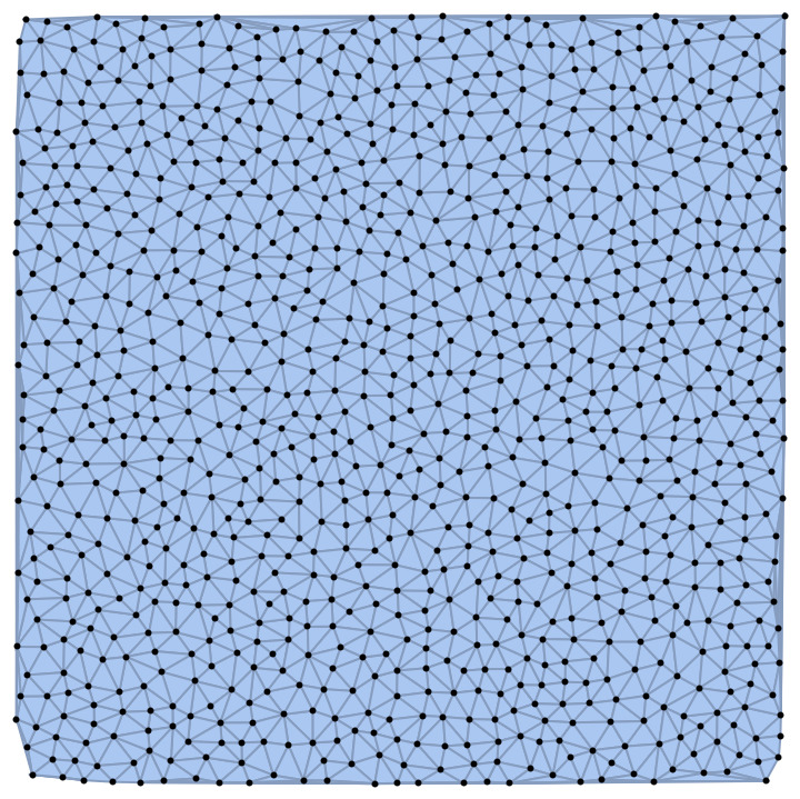
(a) Poisson Disk Sampled Plane

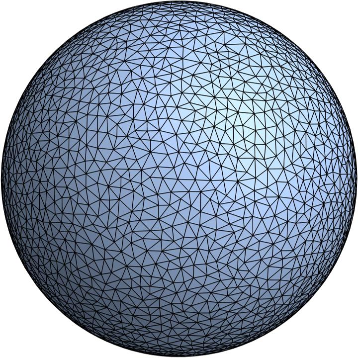
(b) Poisson Disk Sampled Sphere

Figure 1: Delaunay triangulations of a plane and a sphere. The shown Delaunay triangulations are constructed using Python and Mathematica, making use of Poisson disk sampling of points on the surface of smooth 2D surfaces.

We are interested in studying spaces that are large enough to see curvature effects before reaching finite-size effects. To this end, we studied Delaunay triangulations with $150\,\mathrm{k}$ vertices. In the case of the plane this is not as relevant as for the sphere, since we are making a periodic plane using the triangulated square region. In the case of the sphere, we can make a rough estimation of the effective radius of the Delaunay triangulation of the sphere, by comparing the area of the triangulation, given by the number of triangles, to the area of a continuum sphere $4\pi R^{2}$. We set the length of links to $1$, so we estimate the effective radius to be about $R_{\text{eff}}\simeq\sqrt{\frac{\frac{\sqrt{3}}{4}(2*150000)}{(4\pi)}}\simeq 102$. However, after scaling all the links to the same length, the resulting triangulation is further away form the original surface, and is not clear if this is an overestimate, or an underestimate for the area of the closest continuum sphere. The original Delaunay triangulation is close to an equilateral triangulation, which is the case by construction due to the Poisson disk sampling. Still, the triangulation after all edges are taken to be of length $1$ will resemble something more like a "fuzzy" plane or sphere, with bumps everywhere. This "fuzziness" is essential to test the robustness of our curvature definitions, as will be explained later. An example of how this rescaling to equilateral triangles affects the triangulation can be seen in Fig. 2.

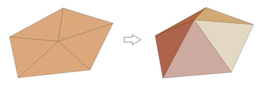
Figure 2: Example of how rescaling all the links to length $1$ affects the geometry of a triangulation. "Cusps" will appear all over the surfaces after rescaling, introducing some "fuzziness" in the triangulated surfaces shown in Fig. 1.

We do this rescaling because we want to measure a discrete version of the generalized curvatures. Since we need to define spheres, it is much more computationally convenient when all link lengths are equal to $1$ since to construct a sphere of radius $r$, one simply needs to find all the points at lattice distance equal to $r$, and the construction of a sphere is straightforward. This would not be the case if the links would have different length between them. Moreover, the building blocks used in 2D CDT are all equilateral, so working with equilateral random surfaces is a natural first step before the using CDT quantum geometries.

There are several ways to discretize the expressions for each $\mathcal{GSC}_{i}$. We decided to discretize all derivatives using second-order accurate finite differences, and to discretize all integrals using a cumulative trapezoidal rule. Specifically, for a function $f(s)$, which we discretize with $f[s]$, where $s=0,1,2,\dots$, we use the discrete derivative

$$\derivative{f}{s}\longrightarrow\begin{dcases}f[1]-f[0]&\text{for }s=0\\ \frac{f[s+1]-f[s-1]}{2}&\text{for }s\geq 1\end{dcases}$$ (14)

and the discrete integral

$$\int_{0}^{s}\differential{s^{\prime}}f(s^{\prime})\longrightarrow\begin{dcases}0&\text{for }s=0\\ \frac{1}{2}\sum_{i=1}^{s}\quantity\Big(f[i]+f[i-1])&\text{for }s\geq 1\end{dcases}.$$ (15)

Additionally, we choose to set $\mathcal{Q}_{p}^{s=0}=0$ in the calculation of the $\mathcal{GSC}_{i}$ to more closely resemble the continuum expressions of the quantities we measure. With this choice, some quotients that appear in the generalized curvatures definitions are ill-defined at $s=0$. In the continuum this is not an issue, because the limit $s\rightarrow 0$ is well-defined; at least for sphere volume and inverse return probability we consider. However, in the discrete setting we cannot take such a limit, and we have to define the value of these quotients that take the form $\frac{0}{0}$, for example $\evaluated{\frac{s\cdot\partial_{s}\mathcal{Q}_{p}^{s}}{\mathcal{Q}_{p}^{s}}}_{s=0}$. Only quotients that appear inside of integrals in our definitions are crucial to define, as they affect the results of the final $\mathcal{GSC}_{i}$ for all $s$. Other ill-defined quotients only affect the results for the first few $s$, in which we are not interested because they are strongly affected by lattice artefacts anyway. Due to the large arbitrariness in defining these quotients, we decided that the most consistent choice with our formalism was setting the value of these ill-defined quotients at $s=0$ to be equal to the value they take in a Riemannian Manifold. The only significant impact this choice makes is on the initial overshoot of the $\mathcal{GSC}$, where nevertheless lattice artefacts dominate. In the case of $\mathcal{GSC}_{i}(\norm{S^{r}_{p}})$ we set

$$\evaluated{\frac{r\cdot\partial_{r}\norm{S^{r}_{p}}}{\norm{S^{r}_{p}}}}_{r=0}=(D-1),\quad\text{and}\quad\evaluated{\frac{\norm{S^{r}_{p}}}{r}}_{r=0}=\begin{dcases}2\pi&D=2\\ 0&D>2\end{dcases},$$ (16)

where $D$ is the topological dimension. In the case of $\mathcal{GSC}_{i}((P_{p}^{n})^{-1})$ we set

$$\evaluated{\frac{n\cdot\partial_{n}(P_{p}^{n})^{-1}}{(P_{p}^{n})^{-1}}}_{n=0}=\frac{D}{2}\quad\text{and}\quad\evaluated{\frac{(P_{p}^{n})^{-1}}{n}}_{n=0}=\begin{dcases}4\pi&D=2\\ 0&D>2\end{dcases},$$ (17)

Notice that an input for ill-defined quotients is only required for the initial point of $\mathcal{GSC}_{2}$, $\mathcal{GSC}_{4}$ and $\mathcal{GSC}_{5}$. In the other cases, the initial point can simply be ignored.

As mentioned before, the numerous prescriptions to define a coarse-grained scalar curvature introduced in Table 1, exist to accommodate the different impacts combinations of derivatives and integrals can have on the numerical results. Numerical integrals tend to be more robust with respect to noise than numerical derivatives, but they have the disadvantage of enlarging short scale lattice artefacts. A balance between introducing large lattice artefacts using integrals, and introducing large noise using derivatives has to be taken into account when implementing the generalized curvatures in a discrete setting. So we present several generalized scalar curvatures $\mathcal{GSC}_{i}$ to be able to compare their features regarding noise and lattice artefacts in discrete implementations. Note that different $\mathcal{GSC}_{i}$ define the same scalar curvature in a smooth Riemannian manifold. However, we cannot take for granted that these multiple definitions are equivalent in a quantum geometry, and we will verify their similarity in the quantum geometries of 2D CDT in the next section.

4.1 Discrete diffusion process

The return probability $(P_{p}^{n})^{-1}$, requires some preliminary explanation of its implementation. First, as mentioned before, if we want to determine precise dimensionful values for the scalar curvature, and not only its signature, we need an identification between the random walk time and the corresponding diffusion time. The identification (9) is based on equally distributed, independent, and integrable Gaussian random variables describing each random step. In the case of a discrete geometry, a standard implementation of a random walk is to start at a point in the space, and move to a random neighbour of that point. The neighbour is chosen uniformly from all direct neighbours. In the case of an irregular discrete space, a vertex might not have the same number of neighbours all other vertices. Therefore, the probability distribution of the random variables determining the random walk is different for each point. To get closer to a situation that best resembles the conditions that allow the identification (9) we will implement the random walk in such a way that each step is equally distributed. This is because, if the variables are not identically distributed, the variance computed in (9) is not necessarily equal to a factor $\sigma^{2}$ times the number of steps taken. In the case of not equally distributed random variables describing each step, relation (9) could be regarded as an effective relation, where the proportionality factor $\sigma^{2}$ would be some effective variance of each step. Since in the case of not equally distributed steps one would have to determine this relation by other means, we will restrict ourselves to a situation where we can compute $\sigma^{2}$ exactly. This is the case of the dual of our triangulations. In the dual lattice of the triangulation, each vertex will have the same amount of nearest neighbours, and thus, the random variables describing each step are equal to a uniform distribution among the three nearest neighbours of each vertex. For a visualization of this effect on a Delaunay triangulation of a sphere and its dual graph, see Fig. 3. If the triangulation is equilateral, ($\sigma^{2}$) can be computed exactly, as we will do later in this chapter.

Even though the random variables in this discrete setting are not Gaussian, we appeal to the Central Limit Theorem and assume that at some large value of $n$ the identification (9) will hold approximately, despite the fact that our variables are uniformly distributed instead of being Gaussians. Therefore, we will use identification (9) for our diffusion processes in the dual lattice, despite the fact that we are not exactly in the situation where this identification is exact. We remark that this implementation in the dual is not necessary if is interested in detecting the presence of curvature by using our prescriptions. The only reason we do this, is because we need a precise identification between diffusion steps and diffusion time, to obtain predictions for the dimensionful numerical value of curvature in our discrete spaces. If one were only interested in determining the presence and signature of curvature in a space, it is sufficient to apply our prescriptions to a diffusion process in the lattice.

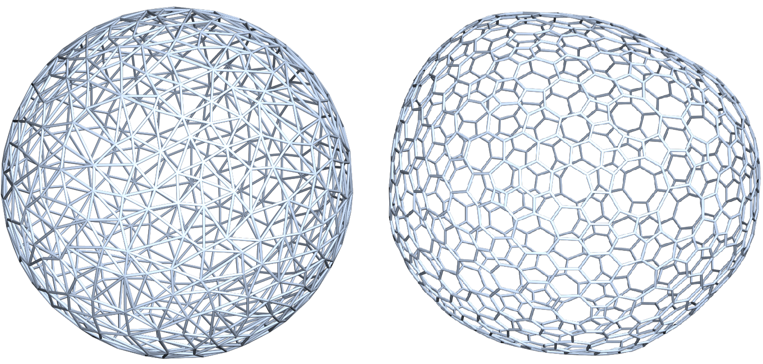
Figure 3: On the left, a Delaunay triangulation of a sphere constructed from a sample of $500$ points on a continuum sphere. On the right, the associated dual graph of the triangulation. Notice that each node in the dual graph has coordination number $3$, even though the vertex graph of the triangulation does not have a fixed coordination number.

Since in the Delaunay triangulation the edge length was set to $1$ everywhere, the edge length in the dual graph is going to be $\frac{1}{\sqrt{3}}$ so in the dual we will also have the same "fuzziness" as in the Delaunay Triangulation. From now on, when we speak of the random walk in the Delaunay triangulations, we will be speaking of a random walk on the dual graph of that Delaunay triangulation, after rescaling all the edges to length $1$.

Let $P(p^{\prime},p;n)$ be the probability of a random walker moving from point $p$ to $p^{\prime}$ on the dual graph of the triangulation, in $n$ steps. We start in our diffusion process with $P(p^{\prime},p;0)=\delta_{p,p^{\prime}}$, where $\delta$ is the Kronecker delta symbol; this signifies that the walk starts at point $p$ and is normalized such that $\sum_{p^{\prime}}P(p^{\prime},p;n)=1$ for all $n$; The diffusion process is then implemented using the evolution equation [16]

$$P(p^{\prime},p;n+1)=(1-\eta)P(p^{\prime},p;n)+\frac{\eta}{3}\sum_{q\sim p^{\prime}}P(q,p;n),$$ (18)

where $q\sim p^{\prime}$ denotes the set of all direct neighbours of $p^{\prime}$ in the graph. Also, $\eta\in\left(0,1\right]$ takes the role of a discrete diffusion constant, which can be set smaller than $1$ to mitigate the large differences between the return probability for odd and even $n$ for small $n$; we use $\eta=0.9$ in our measurements. The return probability is determined by measuring $P_{p}^{n}=P(p,p;n)$ after each diffusion step. If we want to resemble calculations done with the heat kernel, exactly as we did for $||S^{r}_{p}||$, we have to choose scale $n=0$ values for any undetermined ratio that appears in the $\mathcal{GSC}$s.

4.2 Discrete scalar curvature

The results of the implementations for each of the scalar curvatures $\mathcal{GSC}_{i}$, both using $||S^{r}_{p}||$ and $(P_{p}^{n})^{-1}$, on the Delaunay triangulations of a 2-sphere and a periodic plane can be seen in Fig. 4 and 5 respectively. The calculation of the $\mathcal{GSC}_{i}$ is done at each point, for each value of $||S^{r}_{p}||$ and $(P_{p}^{n})^{-1}$. The results for the $\mathcal{GSC}_{i}(||S_{p}^{r}||)$ are more susceptible to the discretization of derivatives and integrals than the $\mathcal{GSC}_{i}((P_{p}^{n})^{-1})$, regarding the initial overshoot and the noisiness of the scalar curvature. For the $\mathcal{GSC}_{i}(||S_{p}^{r}||)$, the dashed line curves in Fig. 4 is a $1$-parameter fit of the continuum curves (see appendix A), where radius is the only fitting parameter ($D=2$). The quality of the fittings depends on the $\mathcal{GSC}_{i}$ in question. The generalized scalar curvatures with more integrals, like $\mathcal{GSC}_{2,3,4}$ seem to fit a constantly curved manifold more closely at large scales. As smaller scales they deviate significantly, due to lattice artefacts. The results for $\mathcal{GSC}_{1,5}$ that contain second derivatives, show precisely the opposite: noise dominates these scalar curvatures at large scales.

Given that the underlying geometry is a sphere, we decided to compute numerical values for the radius instead of the scalar curvature, being equivalent in this situation. The fitted radius of the $\mathcal{GSC}_{i}(||S_{p}^{r}||)$, using the fitting functions provided in appendix A, give $R_{\text{eff},\mathcal{D}}=94.96\pm 0.01$, $R_{\text{eff},\mathcal{I}}=95.367\pm 0.001$, $R_{\text{eff},1}=92.4\pm 5$, $R_{\text{eff},2}=93.97\pm 0.01$, $R_{\text{eff},3}=93.28\pm 0.01$, $R_{\text{eff},4}=93.973\pm 0.001$, and $R_{\text{eff},5}=92.8\pm 0.6$. The error bars presented in the results are simply the errors of the fitting. It is important to remark that since the fitting functions used do not have the initial overshoot present in the numerical results, and are forced to converge to the Riemannian manifold values at short scales, the fitting functions, and therefore the estimated parameters from them, are much more accurate at larger scales than shorter ones. Unfortunately, there is no correct answer, since the triangulation is only topologically a sphere but does not reliably approximate a constantly curved sphere due to the scaling of the edges to be all equal to $1$. The fitting values obtained differ from each others roughly by a $3\%$, and at the most by a $9\%$ from the very rough estimation of $R_{\text{eff}}\simeq 102$ made earlier, where we assumed a sphere perfectly described by equilateral triangles.

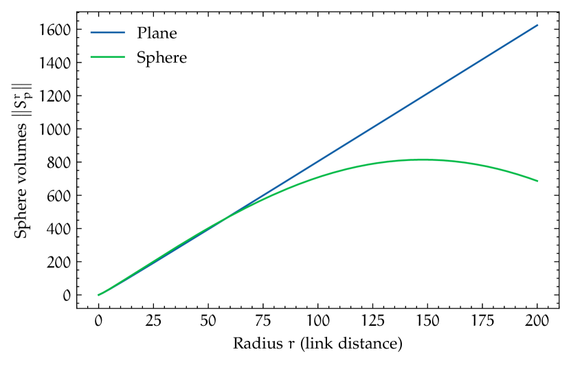
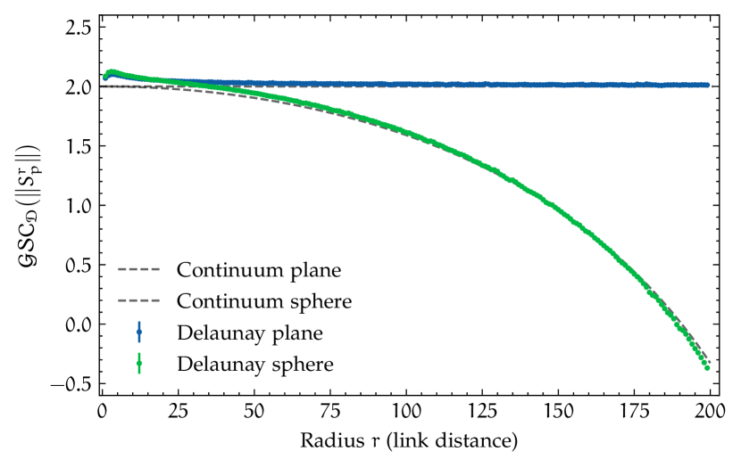
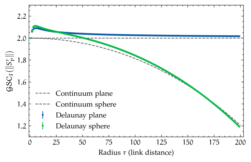
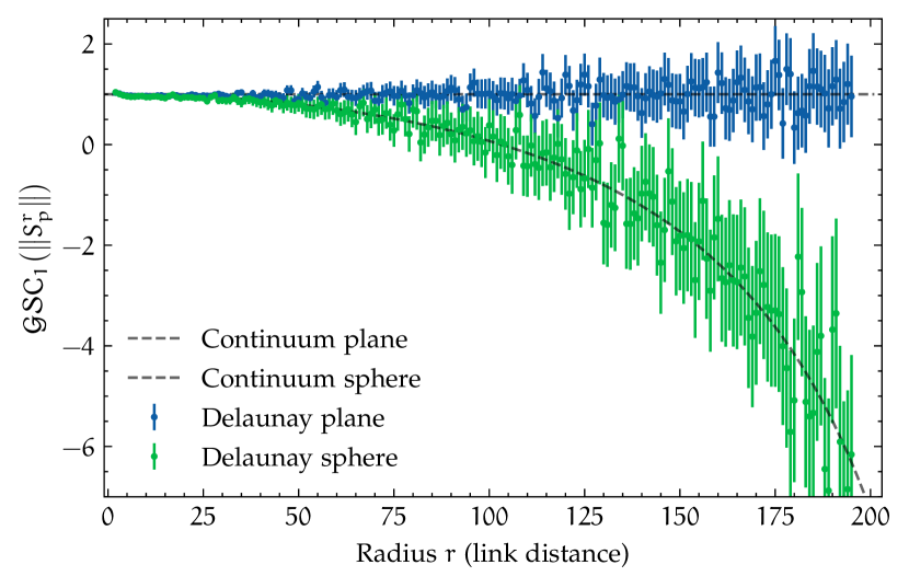
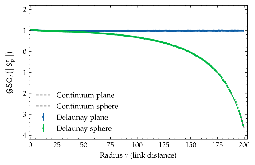
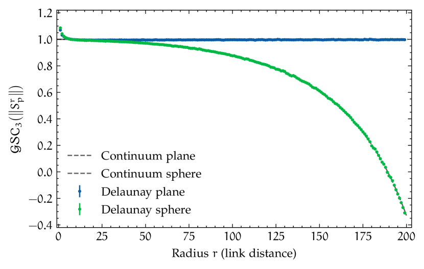
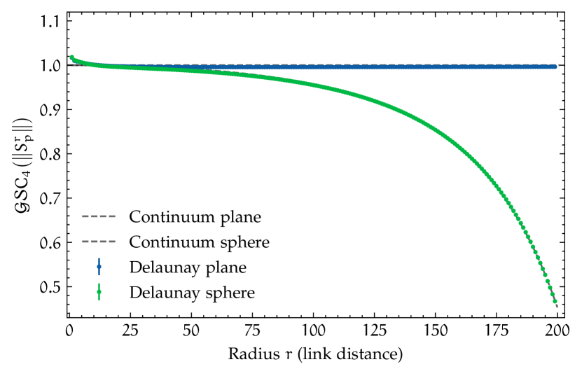
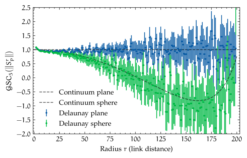
Figure 4: Sphere-volume scalar curvatures $\mathcal{GSC}_{i}(\norm{S_{p}^{r}})$ on a Delaunay triangulation of a plane and sphere of around $150\,\text{k}$ vertices, including the best fit continuum curves for the sphere. The displayed error bars all represent $95\%$-significance or $2\sigma$ intervals, based on the fluctuations between all $20\,\text{k}$ points on the triangulations.

The $\mathcal{GSC}$ are designed for defining curvature, based on small scale properties of scale-dependent quantities like the sphere surface or the return probability, not necessarily by fitting $\mathcal{GSC}_{i}$ with an analytical expression. So we also analyse the small scale behaviour of the measured scalar curvatures to obtain an estimation of the radius of the underlying sphere. To define curvature using the knowledge of the continuum expansion of our $\mathcal{GSC}$, we have to be sure that we are not in a range of lattice artefacts. In our case, we believe that for $\mathcal{GSC}_{\mathcal{I}}(||S_{p}^{r}||)$ and $\mathcal{GSC}_{\mathcal{D}}(||S_{p}^{r}||)$ the size of lattice artefacts seems to be larger than the rest of the $\mathcal{GSC}$. This emphasizes our argument that having this unknown scale-independent prefactor in the observables is an undesired feature. We concluded that lattice artefacts are no longer dominating the numerical results at $r>40$. For $\mathcal{GSC}_{1}(||S_{p}^{r}||)$, $\mathcal{GSC}_{2}(||S_{p}^{r}||)$, $\mathcal{GSC}_{3}(||S_{p}^{r}||)$, $\mathcal{GSC}_{4}(||S_{p}^{r}||)$ and $\mathcal{GSC}_{5}(||S_{p}^{r}||)$, lattice artefacts seem to be negligible for $r>15$. Using this ranges, one can use the knowledge of the expansions (see table 2) to fit a quadratic function to each $\mathcal{GSC}_{i}(||S_{p}^{r}||)$ in the appropriate range, and extract an estimate of the scalar curvature. In this case, we extract the radius of the underlying sphere. Based on the continuum formulas for the $\mathcal{GSC}_{i}(||S_{p}^{r}||)$ in appendix A, we find that for $\frac{r}{R}\leq\frac{1}{2}$, a quadratic approximation of the expansion deviates less than $1\%$ from its actual value for every $\mathcal{GSC}_{i}(||S_{p}^{r}||)$. So, it can be used as a decent approximation to compute the curvature in this range. In this range we estimate the scalar curvature as

$$\frac{\mathcal{SC}_{i}(||S_{p}^{r}||)}{\beta_{i}(D)\,r^{2}}\simeq R_{p}+\mathcal{O}(r^{2}),$$ (19)

where

$$\beta_{i}(D)=\{\frac{-1}{3D},\frac{-1}{3(2+D)},\frac{-2}{3D},\frac{-2}{9D(D-1)},\frac{-2}{3D^{2}(D+2)},\frac{-2}{3D^{5}+6D^{4}-3D^{3}-6D^{2}},\frac{-8(D-1)}{9D}\}$$

$$\quad\text{for }i=\{\mathcal{D},\mathcal{I},1,2,3,4,5\}$$ (20)

We decided to apply this approximation to the value of $r=50$ in all our $\mathcal{GSC}_{i}(||S_{p}^{r}||)$ using $D=2$. We chose this radius since we believe that it is the smallest value of $r$ at which all $\mathcal{GSC}_{i}$ can be assumed to have negligible lattice artefacts. The large value is due to $\mathcal{GSC}_{3}(||S_{p}^{r}||)$ and $\mathcal{GSC}_{4}$, that posses a large range of lattice artefacts. With the obtained value of the curvature $R_{p}$, one can estimate the more intuitive dimensionful value, which is the associated effective radius defined as $R_{p}\doteq\frac{D(D-1)}{R_{eff}^{2}}$, that provides an estimation for the size of the approximate sphere being triangulated. The results for the estimations of $R_{\text{eff}}$ are $R_{\text{eff},1}=85\pm 16$, $R_{\text{eff},2}=81\pm 1$, $R_{\text{eff},3}=85\pm 1$, $R_{\text{eff},4}=75\pm 1$, and $R_{\text{eff},5}=84\pm 11$, where $R_{\text{eff},i}$ denotes the estimate of $R_{\text{eff}}$ based on the results of $\mathcal{GSC}_{i}$. The error bars presented for the estimated effective radius are the propagated errors coming form the statistical error in the $\mathcal{GSC}_{i}$s. Except for the estimated radius using $\mathcal{GSC}_{4}$, the other estimations agree with each others within error bars. We believe that the significant deviation in the estimation of $R_{\text{eff},4}$ comes from the fact that the two integrals involved introduce, small, but non-vanishing discretization artefacts even at large scales. This renders $\mathcal{GSC}_{4}$ not suitable for estimations of the curvature using approximation (19). Other sources of error, like a systematic error from the truncation to a quadratic function, or a method that takes into account how different our equilateral triangulation is from a continuum sphere might change these results, making them overlap with each others and with the global fit used previously. Later, we will see that the results using the return probability are more accurate, and overlap with each others and with the global fit of the continuum sphere. Note that in this case $i=\mathcal{D},\mathcal{I}$ cannot be used at this short distance $r=50$ as the lattice artefact are large for these $\mathcal{GSC}$, such that each $\mathcal{GSC}$ is still to strongly deviating from the continuum result at $r=50$.

This would correspond to a significantly larger or even negative curvature, so we will not associate a sphere radius in these cases. This means $\mathcal{GSC_{D}}$ and $\mathcal{GSC_{I}}$ are not well suited for extracting the scalar curvature using (19). We believe the main reason for this is the leading unknown constant different from $1$ that dominates the numerical value of $\mathcal{GSC_{D}}$ and $\mathcal{GSC_{I}}$. This emphasizes the use of the other five methods to determine the curvature of the underlying space, since they do not contain this unknown leading constant by construction.

Unfortunately, the quadratic approximations for every $\mathcal{GSC}_{i}(||S_{p}^{r}||)$ are not good approximations if we compare the results with the global fit obtained from the continuum formulas. At the used scales, they provide the effective radius with an error of roughly $10\%$, compared with the continuum fit. Furthermore, since the results coming from some of them don’t overlap with each others, it is difficult to determine which one is the most suitable for such approximation. This means that estimations of the curvature using a quadratic approximation of $\mathcal{GSC}_{i}(||S_{p}^{r}||)$ are nor numerically reliable. They can provide an estimate of the actual curvature radius, but one should be aware that, at least in the scales analysed in this work, there is roughly a $10\%$ error when estimating the effective radius. We therefore conclude that the $\mathcal{GSC}_{i}(||S_{p}^{r}||)$ are more useful for determining large scale curvature, by comparing the continuum formulas with the numerical results obtained, instead of being precise for determining curvature at each point. This picture changes when studying $\mathcal{GSC}_{i}((P_{p}^{n})^{-1})$.

Overall, our conclusion is that the $\mathcal{GSC}_{2}(||S_{p}^{r}||)$ is the most robust definition of curvature in this case. The reason is that $\mathcal{GSC}_{2}(||S_{p}^{r}||)$ seems to have less noise at large scales than the $\mathcal{GSC}_{i}(||S_{p}^{r}||)$ with two derivatives, and at small scales, the curved and the flat manifold cases start deviating from each other faster than the $\mathcal{GSC}_{i}(||S_{p}^{r}||)$ with two integrals. Furthermore, as shown in appendix A, $\mathcal{GSC}_{2}(||S_{p}^{r}||)$ has the property of being independent of the dimension of the space in a constantly curved $D$-dimensional manifold. This makes it ideal to apply in fractal spaces where the dimension is unknown, and very useful to compare with constantly curved spacetimes. Whether this holds for more general manifolds is unknown to us.

In Fig. 5, we discuss the results of $\mathcal{GSC}_{i}((P_{p}^{n})^{-1})$, after averaging over a sample of $200$ points, to eliminate the "fuzziness". There is an overall increase in the robustness of the generalized scalar curvatures compared to using the sphere surface. Furthermore, we studied diffusion steps up to values $2$ orders of magnitude larger than the lattice distance used with the sphere surface. Nonetheless, we see that the measured range shows only a linear correction to flatness; an exception is $\mathcal{GSC}_{1}$, where we see higher-order corrections at the largest measured scales. Therefore, it seems that the diffusion process explores distance scales much smaller than the sphere surface. Because of that, it became computationally unfeasible to study equivalent distance scales with both methods. This is not a problem, since both methods can be used complementary to study different scale ranges in more detail in the same metric space. This indicates that $\mathcal{GSC}_{i}((P_{p}^{n})^{-1})$ is ideal to define the scalar curvature at short scales, since the higher-order contributions are negligible until large diffusion times.

Given that there is no closed formula for the return probability on a sphere, only asymptotic expansions, we do not have closed analytical expression of $\mathcal{GSC}_{i}((P_{p}^{n})^{-1})$ to fit to. Nevertheless, we can still estimate the curvature and the radius of the underlying sphere using the formula

$$\frac{2\eta}{\sigma^{2}}\frac{\mathcal{SC}_{i}((P_{p}^{n})^{-1})}{\gamma_{i}(D)\,n}\simeq R_{p}+\mathcal{O}(n^{2}),$$ (21)

where

$$\gamma_{i}(D)=\{\frac{-1}{6},\frac{-(2+D)}{6(4+D)},\frac{-1}{6},\frac{-1}{6D},\frac{-2}{3(8+6D+D^{2})},\frac{-8}{3D(2+D)^{2}(4+D)},\frac{-D}{8}\}$$

$$\quad\text{for }i=\{\mathcal{D},\mathcal{I},1,2,3,4,5\}$$ (22)

We apply this approximation for all $\mathcal{SC}_{i}((P_{p}^{n})^{-1})$ using $D=2$, and at $n=5000$, because we believe it is roughly the smallest value of $n$ at which lattice artefacts can be neglected in all profiles.

To estimate of the effective radius of the underlying sphere, we have to determine the value of the standard deviation $\sigma^{2}$ in (9).

In the dual of a triangulation, this value can be computed exactly, to be $\sigma^{2}=\frac{1}{3}$.

This leads us to the following estimations of the radius of the sphere from formula 21, $R_{\text{eff},\mathcal{D}}=102\pm 4$, $R_{\text{eff},\mathcal{I}}=109\pm 7$, $R_{\text{eff},1}=96\pm 4$, $R_{\text{eff},2}=91\pm 4$, $R_{\text{eff},3}=91\pm 4$, $R_{\text{eff},4}=100\pm 8$, and $R_{\text{eff},5}=94\pm 4$, where $R_{\text{eff},i}$ denotes the estimate of $R_{\text{eff}}$ based on the results of $\mathcal{GSC}_{i}$.

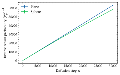
(a)

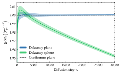
(b)

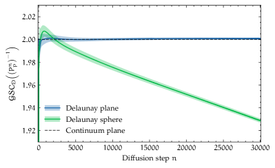
(c)

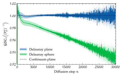
(d)

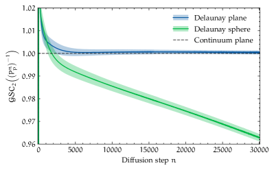
(e)

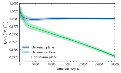
(f)

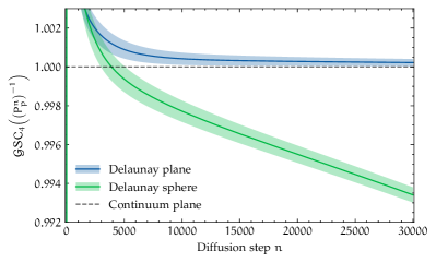
(g)

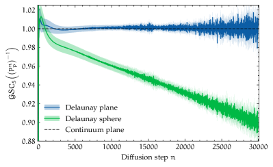
(h)

Figure 5: Scalar curvature on a Delaunay triangulation of a plane and sphere based on inverse return probability. The continuum plane curve indicates what flat curvature looks like in the underlying continuum plane. The error bands give a $95\%$-confidence interval, which is based on the fluctuations between $50$ points on the triangulations.

Except for the predictions using $\mathcal{GSC}_{\mathcal{D}}((P_{p}^{n})^{-1})$ and $\mathcal{GSC}_{\mathcal{I}}((P_{p}^{n})^{-1})$, these values are close to the estimated values obtained from the continuum fit formulas using sphere surface, and we interpret these results as a confirmation of the robustness of the method and of our definitions. Furthermore, these results overlap with each others within error bars and are also close to the rough expectation of $R_{\text{eff}}\simeq 102$ mentioned before. Besides, also using this spectral method to determine the curvature, $\mathcal{GSC}_{\mathcal{D}}((P_{p}^{n})^{-1})$ and $\mathcal{GSC}_{\mathcal{I}}((P_{p}^{n})^{-1})$ deviate larger from the rest, as was to be expected since the leading constant of these quantities is in principle undetermined, emphasizing the fact that they are not suitable for extracting the scalar curvature, at least using the return probability.

The range where the initial lattice artefacts dominate is in accordance with the range where lattice artefacts disappeared using the sphere surface. To see this, one can make use if identification 9 and determine the approximated relation between $r$ and $n$ as $\operatorname{Var}\quantity(S_{n})=\sigma^{2}n\simeq r^{2}$. Since in case of using the sphere surface the lattice artefacts disappeared in a range between $r=35$ and $r=40$, this means that lattice artefacts for the return probability should disappear in a range between $n=3675$ and $4800$, precisely as wee observe in our measurements.

All the generalized scalar curvatures exhibit noise at large scales, and we observe no significant difference between the small scale lattice artefacts among them. So, we conclude that $\mathcal{GSC}_{5}((P_{p}^{n})^{-1})$ is the best to measure scalar curvature, because of its linearity at a large range of scales and for having the largest absolute deviation from constancy, with respect to the other $\mathcal{GSC}_{i}((P_{p}^{n})^{-1})$ with no unknown leading constant.

Ideally, used together, $\mathcal{GSC}_{i}((P_{p}^{n})^{-1})$ will prove short scale distance curvature, and $\mathcal{GSC}_{i}(||S_{p}^{r}||)$ will prove larger distance scales, providing a large range of scales at which scalar curvature can be defined and computed in a metric space. If one is interested in the large scale geometry of the space, then we suggest to use $\mathcal{GSC}_{2}(||S_{p}^{r}||)$, and compare the results with the constantly curved manifold profiles. If one is interested in a more detailed information about the curvature at short scales, like to measure correlations of scalar curvature at two different points, then we suggest to use $\mathcal{GSC}_{5}((P_{p}^{n})^{-1})$.

One last remark is in order. We expect that the numerical differences in the estimation of the scalar curvature between the $7$ different $\mathcal{GSC}$s disappears when taking the limit of vanishing lattice spacing. Since we did not perform a study of the scaling of our results at different triangulation volumes, this remains a conjecture.

In what follows, we will use these definitions to determine the curvature of the quantum geometries that appear in the path integral of 2D Causal Dynamical Triangulations. Since these geometries are also triangulations, we use the same prescriptions as used for the Delaunay triangulations in this section.

5 Quantum scalar curvature

As discussed in the introduction, the main motivation for our generalized definitions of curvature is its use in a quantum geometry setting. Here, there is no notion of tensor calculus, but we can define distances and a diffusion process. In order to create valid observables for the quantum geometries it must be diffeomorphism invariant, which means that point dependence has to be eliminated. This is because the points in the quantum geometries are fluctuating, and no identification between points in different configurations can be made. As such, we will define an average quantum scalar curvature observable, for which we will remove the point dependence of our curvature definitions by taking a manifold average. To that end, we define the Quantum Scalar Curvature $\mathcal{QSC}_{i}(\mathcal{Q}^{s})$ based on an $s$ scale-dependent local observable $\mathcal{Q}_{p}^{s}$ to be:

$$\mathcal{QSC}_{i}(\mathcal{Q}^{s})=\frac{\int\differential[D]{p}\sqrt{\absolutevalue{g}}\,\mathcal{GSC}_{i}(\mathcal{Q}_{p}^{s})}{\int\differential[D]{p}\sqrt{\absolutevalue{g}}},$$ (23)

where the manifold average is taken over manifold $M$ with metric $g$, where $\absolutevalue{g}$ denotes the metric determinant. Then, we want to compute the expectation value of this quantum scalar curvature $\mathcal{QSC}_{i}(\mathcal{Q}^{s})$ observable,

$$\expectationvalue{\mathcal{QSC}_{i}(\mathcal{Q}^{s})}=\frac{1}{Z}\int\mathcal{D}\quantity[g]\,e^{-S_{\text{eu}}[g]}\,\mathcal{QSC}_{i}(\mathcal{Q}^{s}),$$ (24)

which is the Euclidean expectation value given as a Euclidean path integral over all possible geometries. The measure $\mathcal{D}[g]$ here, denotes that the integral is taken over distinct geometries, which is given by the measure over all metrics $\mathcal{D}g$, dividing out the diffeomorphisms of the geometry [17]. The Euclidean action $S_{\text{eu}}(g)$ is dictated by the particular model one is working with. Furthermore, we denote the partition function as $Z=\int\mathcal{D}\quantity[g]\,e^{-S_{\text{eu}}[g]}$. For this paper we choose the setting of two-dimensional Causal Dynamical Triangulations (CDT) [18].

In general, CDT is a non-perturbative method to quantize gravity. It uses lattice techniques to regularize the sum over all possible metrics on a manifold, by replacing and defining it as a sum over all possible simplicial discretizations of it, with some constraints on the possible gluings between the constituting simplices. These constraints are the ones responsible for allowing a well-defined Wick rotation in CDT, unlike other approaches where sometimes it is not even clear if this rotation exists. The causal dynamical triangulations in the name of the approach are the simplicial manifolds that represent curved, Lorentzian spacetimes appearing in the gravitational path integral. The causality is imposed by a distinction between time and space like edges of the simplices, and a particular way of gluing them such that at each point there is a foliation of the space in the direction of the time-like edges. By gluing these simplices, one obtains a simplicial manifold. Using these discrete elements one can actually make sense of the path integral over all geometries. The study of the resulting (discrete) quantum geometries is usually done by means of Monte Carlo simulations. With the use of these simulations, one can generate an ensemble of path integral configurations, where each of them will be a simplicial manifold, and therefore a discrete geometry. The expectation value of an observable over this ensemble, is later on approximated by an average over a sample of configurations in this ensemble. The ensemble of all these path integral configurations constitutes the so-called quantum geometry under study.

Since it is out of the scope of this work to properly introduce all the details of CDT, we refer the reader to some extensive reviews on the matter [19, 2]. What the reader should retain from this brief and incomplete introduction to CDT, is that from the CDT simulations, one can obtain an ensemble of discrete geometries constituting a quantum geometry, where the main interest is to study its geometrical properties, like curvature.

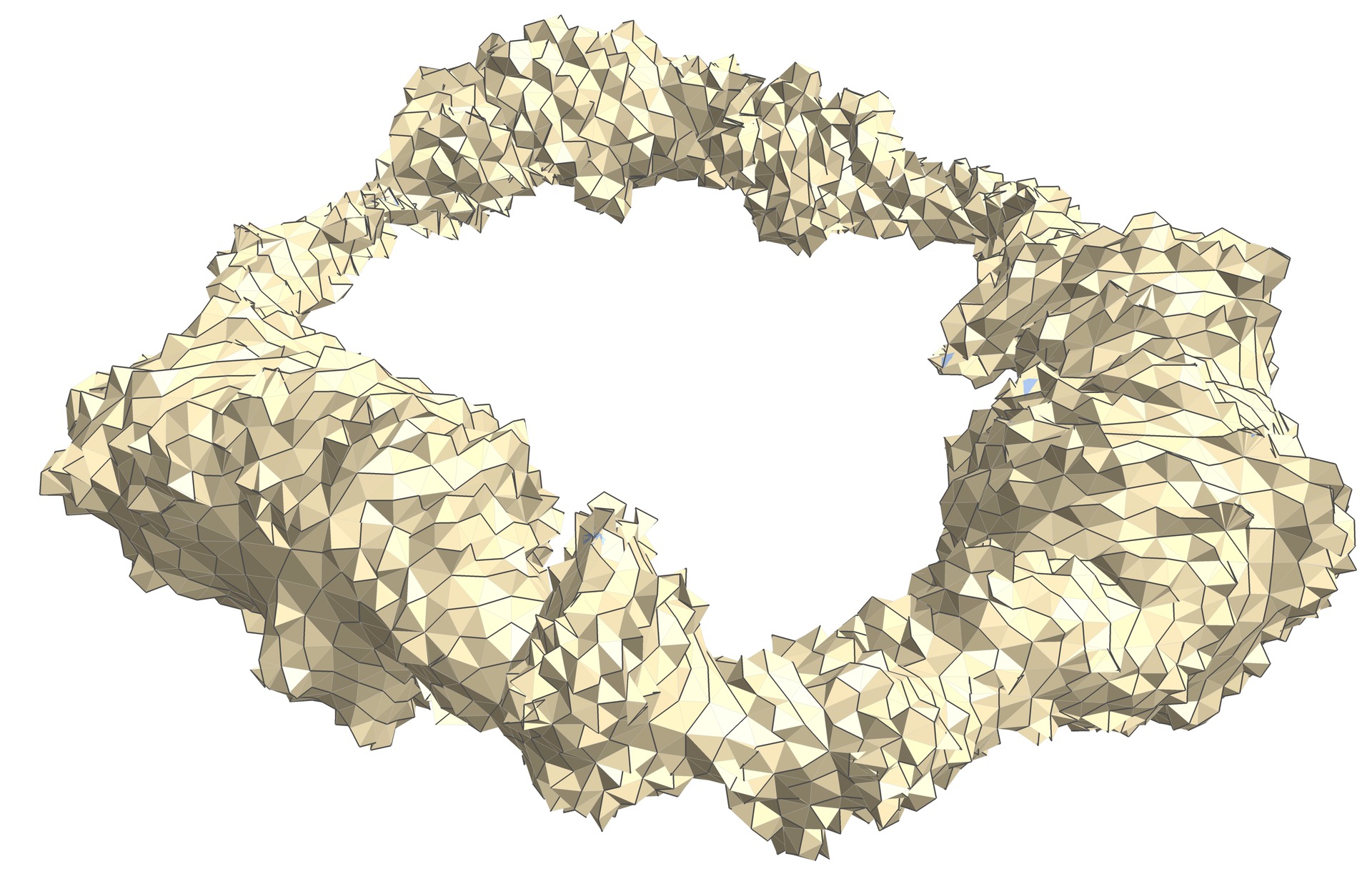
Figure 6: Visualization of a typical triangulation of 2D CDT with $N_{2}=10\,{k}$ triangles and $\tau=123$ time-slices, based on a spring embedding. Spatial slices of constant time are marked by dark lines.

In two-dimensional dynamical triangulations, the discretized version of the Einstein-Hilbert action becomes very simple. In this case the Euclidean action for a given triangulation $T$ is given by: $S_{\text{DT}}(T)=\lambda N(T)$, where $\lambda$ is a dimensionless cosmological constant and $N(T)$ is the number of triangles in the triangulation. The partition function over the ensemble $\mathcal{T}$ is given by

$$Z=\sum_{T\in\mathcal{T}}\frac{1}{C_{T}}e^{-\lambda N(T)},$$ (25)

where $C_{T}$ is a symmetry factor suppressing highly symmetric triangulation. In this case, the expectation value of the quantum scalar curvature is defined as

$$\expectationvalue{\mathcal{QSC}_{i}(\mathcal{Q}^{s})}=\frac{1}{Z}\sum_{T\in\mathcal{T}}\frac{1}{C_{T}}e^{-\lambda N(T)}\,\frac{1}{\absolutevalue{T}}\sum_{p\in T}\mathcal{GSC}_{i}(\mathcal{Q}^{s}_{p}),$$ (26)

where $\absolutevalue{T}$ is the total number of points $p$ in the vertex (or dual) graph of the triangulation. Instead of considering the ensemble of all triangulations, we consider the ensemble of triangulations with a fixed total volume $N(T)=N_{2}$. This fixed-volume ensemble is much more convenient to work with computationally, making it the standard choice for numerical CDT [19]. Furthermore, we only consider triangulations with a toroidal topology without boundaries.

As mentioned before, we estimate the quantum scalar curvature by sampling triangulations from the ensemble using Markov chain Monte Carlo methods. It is possible to compute the triangulation average of $\mathcal{GSC}_{i}(\mathcal{Q}^{s}_{p})$ in each triangulation, but computationally rather expensive. Instead, we estimate the triangulation average with a sample average, based on a uniform sample of points. To decrease the effect caused by the compactness of the geometry we perform the actual measurements on an unwrapped version of the simulation toroidal triangulations. Specifically we cut the triangulations open along two closed non-contractible loops and tile the unfolded triangulation to create an infinite periodic triangulation of planar topology; for more details see [20].

Identical to the implementation in the Delaunay triangulations, the sphere volume measurements are implemented by counting the number of points in vertex graph at a given link distance $r$ from the origin. The computation of the return probability of a random walker is also implemented in the way as for the Delaunay triangulations. We use the dual graph of the CDT triangulations and perform the random walk by updating the probability of the random walk with (18). The return probability at a point $p$ after $n$ steps in a configuration $T$, is computed by recording the value of $P_{T}(p,p;n)$ after each diffusion step in (18).

Using the described methods we measured the quantum scalar curvatures for sphere volumes $||S_{p}^{r}||$ in CDT. We performed measurements on $5\,{k}$ triangulations and approximated the manifold average by a sample average over $500$ points. The resulting quantum scalar curvatures are displayed in Fig. 7.

From Fig. 7 we see some interesting features of the resulting quantum scalar curvatures. First, all of them exhibit a plateau. This means that all prescriptions are compatible with a zero curvature space. This is remarkable and is not to be expected a priori, since the configurations themselves are by no means something one would consider flat. In fact, a typical configuration of toroidal topology looks like Fig. 6.

One remark is in order. The measured values for $\mathcal{GSC}_{\mathcal{D}}(||S_{p}^{r}||)$ and $\mathcal{GSC}_{\mathcal{I}}(||S_{p}^{r}||)$ have a plateau at a value different from $2$, and the plateau is rather at around $\simeq 2.2$. Furthermore, the expectation value $\expectationvalue{||S_{p}^{r}||}$ differs greatly from the $2$-dimensional Delaunay plane and sphere.

There are two reasons for this. First, as mentioned before, the multiplying factor to $||S_{p}^{r}||$ is unknown, and can be different in different spaces, changing the absolute value of $||S_{p}^{r}||$ in different discrete spaces. Furthermore, from $\mathcal{GSC}_{\mathcal{D}}(||S_{p}^{r}||)$ and $\mathcal{GSC}_{\mathcal{I}}(||S_{p}^{r}||)$ one can see that the expectation value of the parameter determining the leading power is not exactly equal to $2$ but rather $\simeq 2.2$. This parameter can be interpreted as the scaling dimension of the geodesic spheres, and by fitting a power law directly to the expectation value of $||S_{p}^{r}||$ one extracts the so called Hausdorff dimension.

(a)

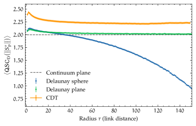
(b)

(c)

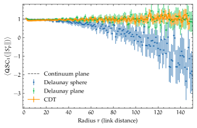
(d)

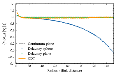
(e)

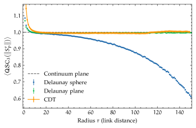
(f)

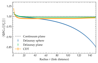
(g)

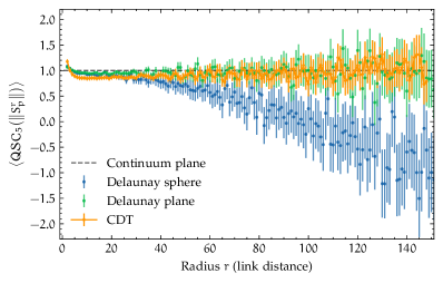
(h)

Figure 7: The quantum scalar curvatures of the sphere volume $\expectationvalue{\mathcal{QSC}_{i}(\norm{S_{p}^{r}})}$ on 2D CDT with $N_{2}=300\,\text{k}$ triangles and $\tau=219$ time-slices. As a comparison the generalized scalar curvature results $\mathcal{GSC}_{i}(\norm{S_{p}^{r}})$ of the Delaunay triangulations as already presented in Fig. 4 are also included with the same number of triangles, $300\,\text{k}$, as well as the continuum expectation for a plane, reflecting no curvature. The error bars represent $95\%$-confidence intervals; for CDT this is based on the fluctuations in $\mathcal{QSC}_{i}$ over $5000$ CDT configurations.

The theoretical value for the Hausdorff dimension in 2D CDT is $2$, but it has been shown that is remarkably difficult in simulations to recover this value numerically. This seems to be the case in our observables, where our leading scaling parameter is also not exactly equal to $2$ as expected from the topological dimension of the triangulation. Since this is only a problem for determining the curvature from $\mathcal{GSC}_{\mathcal{D}}$ and $\mathcal{GSC}_{\mathcal{I}}$, but not from the rest of the $\mathcal{GSC}_{i}$s, and since it is outside the scope of this work to dive into the details of the dimension of these fractal spaces, we refer the reader previous investigations in the calculation of the Hausdorff dimension, and other notions of dimensions [19, 16, 21, 22]. The fact that after our manipulations the generalized curvatures between CDT and the Delaunay plane overlap, despite having possible different leading powers and different leading multiplying constants is a confirmation that our manipulations and definitions indeed eliminate these differences, keeping only the curvature scale dependent contributions.

In conclusion, all our measurements of $\mathcal{GSC}_{i}(||S_{p}^{r}||)$ seem to indicate that, at least up to the measured scales, the ground state of the 2D CDT path integral exhibits the properties of a space with zero average curvature, when extracting curvature using the geodesic sphere surface.

Similarly, we performed measurements of the quantum scalar curvature based on the inverse of the return probability $(P^{n}_{p})^{-1}$, measured using the previously described methods. We performed measurements on $1370$ triangulations of the fixed-volume ensemble, and we approximated the manifold average by a sample average over $100$ points. The resulting $\mathcal{QSC}_{i}((P^{n}_{p})^{-1})$ are presented in Fig. 8. Similar to the sphere volume measurements we see that after a region of discretization artefacts the $\mathcal{QSC}_{i}((P^{n}_{p})^{-1})$ are compatible with flatness within error bars, again indicating $0$ average curvature. Compared to the QSC based on sphere volumes the statistical errors are a smaller in absolute terms, even though a lot less samples are used. This seems to indicate that using the return probability is more robust than using the sphere surface. Nevertheless, we also see in this case, that there are large overshoots for every $\mathcal{GSC}_{i}((P^{n}_{p})^{-1})$ at $n<1000$. Even though in absolute value these deviations are rather small, one should also take into account that extracting the curvature using this method one will always obtain very small deviations from $1$. In particular, we saw that for a Delaunay triangulation of a sphere with the same number of triangles, the deviations from $1$ where roughly up to $0.1$, which means that lattice artefacts of this order are large. Despite this, at $n>5000$ these effects seem to be washed out, and results compatible with flatness were found. Interestingly, unlike in the case of the sphere surface, $\mathcal{GSC}_{\mathcal{D}}((P^{n}_{p})^{-1})$ and $\mathcal{GSC}_{\mathcal{I}}((P^{n}_{p})^{-1})$ seem to have a plateau at a value much closer to $2$ than the ones using the sphere surface, indicating that using a random walker, the leading power of the return probability is compatible with a spectral dimension of 2D CDT to be equal to $2$ (recall the leading term in each $\mathcal{GSC}$ in Tab. 2). Nevertheless, if one were to fit a constant value to the results of $\mathcal{GSC}_{\mathcal{D}}((P^{n}_{p})^{-1})$ and $\mathcal{GSC}_{\mathcal{I}}((P^{n}_{p})^{-1})$, it would be slightly above $2$. This slight deviation in the leading power of $(P^{n}_{p})^{-1}$, together with a difference in the leading multiplying factor of $(P^{n}_{p})^{-1}$ between different discrete spaces, can also be seen in the plots of $(P^{n}_{p})^{-1}$, where one can see deviations from the Delaunay plane. Again, the fact that after our manipulations the generalized curvatures between CDT and Delaunay plane overlap despite having possible different leading powers and different leading multiplying constants, is another confirmation that our manipulations and definitions indeed eliminate these differences, keeping only the curvature scale dependent contributions.

Summarizing, we conclude that all our definitions of scalar curvature indicate that the path integral ground state of 2D CDT has average curvature equal to $0$. This could go in contradictions with the studies performed in [23], where it was found that the QRC measured in 2D CDT seemed to be non-constant. Their result could either indicate the presence of curvature, or of some slowly decaying lattice artefact, that vanishes for scales larger scales than the ones studied in [23]. Despite the remarkable precision in their measurements, the QRC still has the problem of the unknown leading prefactor multiplying the results, as mentioned in the introduction. The problem in interpreting the results of the QRC, is that even if a non-constant region of the scale-dependent QRC is observed, one does not know how far away from flatness it is. Therefore, the actual numerical value of the QRC is meaningless unless one knows the multiplying prefactor, and because of that, one cannot know if the results are actually converging to it or diverging from it.

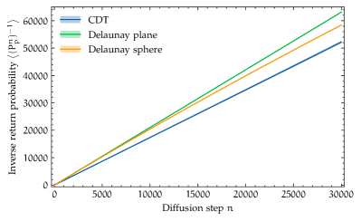
(a)

(b)

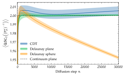
(c)

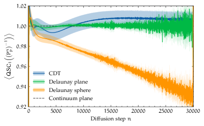
(d)

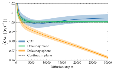
(e)

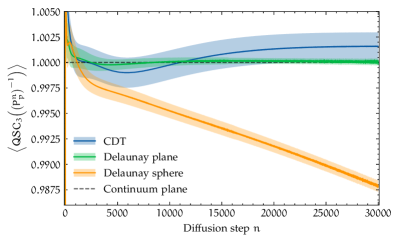
(f)

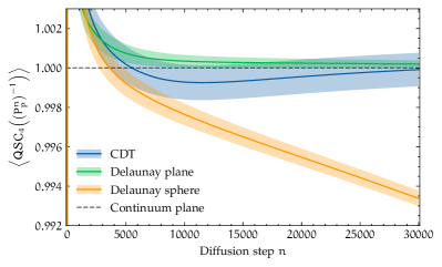
(g)

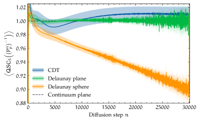
(h)

Figure 8: The quantum scalar curvatures of the inverse return probability $\expectationvalue{\mathcal{QSC}_{i}((P_{p})^{-1}))}$ on 2D CDT with $N_{2}=300\,\text{k}$ triangles and $\tau=219$ time-slices. As a comparison the generalized scalar curvature results $\mathcal{GSC}_{i}(\norm{S_{p}^{r}})$ of the Delaunay triangulations as already presented in Fig. 4 are also included with the same number of triangles, $300\,\text{k}$, as well as the continuum result for generalized scalar curvature in a plane. The error bands represent $95\%$-confidence intervals; for CDT this is based on the fluctuations in $\mathcal{QSC}_{i}$ over $1370$ CDT configurations, and for the Delaunay triangulations this is based on the fluctuation between $50$ different points on the triangulation.

We believe that we have solved that problem in our curvature definitions, by eliminating this unknown leading constants and powers. This is because by construction, since our observables are ratios of derivatives or integrals of the same quantity, any multiplying scale independent factor disappears, leaving only the scale-dependent part of it. Furthermore, even if the leading scaling power is unknown, $\mathcal{GSC}_{i}$ with $i=1,2,3,4,5$ will also eliminate this leading scaling, preserving only the curvature contributions of the quantity used. In these generalizations of the scalar curvature, the reference value is always $1$, independently of the used quantity. This makes the interpretation of the results easier than in the presence of unknown leading powers or multiplying constants, since any deviation from $1$ is interpreted as the presence of curvature, and its sign depends on the quantity being used.

6 Conclusions

In this paper we define and implement generalized notions of Ricci scalar curvature, for metric spaces endowed with a measure and/or with a random walk, with the aim of providing computationally feasible methods of determining curvature that can be implemented in the non-perturbative approach to quantum gravity called Causal Dynamical Triangulations (CDT). The definitions are successfully implemented in 2D CDT. This is done without the need of defining or computing intermediate, more complex, quantities like the Riemann or Ricci tensor. We do not assume the existence of tensor calculus at any stage in our definitions of curvature in these spaces. Moreover, our constructions do not assume that the considered spaces are smooth in any sense. Indeed, they are designed to be used in discrete and fractal spaces, like the ones appearing in CDT. Furthermore, our definitions are made intentionally without the use of coordinates, since this is situation that is encountered in the geometries of CDT.

For the construction of these generalized notions of scalar curvature $\mathcal{GSC}$, we use quantities that can be computed both in a Riemannian manifold, and in a metric space with a measure and/or a random walk. In particular, we use the volume of a sphere $||S_{p}^{r}||$ with a radius $r$, centred at a point $p$, and we use the return probability $P_{p}^{n}$ of a random walker at a point $p$ after $n$ steps. In a Riemannian manifold, both of these quantities define the Ricci scalar curvature by the leading-order scale-dependent correction from the result in Euclidean space. In a nutshell, the procedure used to define a $\mathcal{GSC}$ is the following: 1) Find a scale dependent quantity that can be computed both in a Riemannian manifold and in a metric space with a measure and/or a random walk. This quantity should be such that in a Riemannian manifold, its first curvature correction with respect to the Euclidean calculation defines the Ricci scalar. Examples are $||S_{p}^{r}||$ and $P_{p}^{n}$. 2) Apply a certain number of integrals and derivatives to this scale dependent quantity, to extract the leading order curvature correction in a Riemannian manifold. 3) Replicate these calculations on the metric space in question, and use the result as a definition of scalar curvature, associated with this quantity.

Our definitions, for a general scale-dependent quantity, are shown in table 1. Their expansions in a Riemannian manifold, using $||S_{p}^{r}||$ and $P_{p}^{n}$, are shown in table 2. We introduce $7$ different methods, that involve different combinations of integrals and derivatives. The reason for doing this is that different methods introduce different undesired numerical effects like noise and lattice artefacts in discrete spaces. The methods are compared in order to find the one that has the most desirable features, which can be different in a different setting. We tested these definitions on random geometries generated by constructing Delaunay triangulations of a sphere and a periodic plane. Our results seemed to indicate that applying these prescriptions to determine the generalized scalar curvature of the corresponding Delaunay triangulations, match remarkably well with the Ricci scalar of the underlying Riemannian manifolds. We conclude that this is a confirmation that our generalized notions of curvature can indeed be applied reliably to discrete metric spaces, and that their result can be interpreted as a notion of scalar curvature.

To determine the curvature of the ground state of the path integral in 2D Causal Dynamical Triangulations, we also measured our generalized notions of scalar curvature in this setting. We estimated the expectation value of our $\mathcal{GSC}$s associated with $||S_{p}^{r}||$ and $P_{p}^{n}$, and determined that the expectation value of all of our curvature definitions, both using $||S_{p}^{r}||$ and $P_{p}^{n}$, are compatible with flatness. This seems to suggest that the ground state of the 2D CDT path integral is flat. The results are shown in Fig. 7 and 8.

Despite the fact that in a Riemannian manifold, all our generalized scalar curvatures are equivalent in the sense that they all define the Ricci scalar curvature at small scales, we conclude that two of our definitions of curvature are better than the others in the discrete cases we considered. Our conclusions are based in the implementations on the Delaunay triangulations. We considered as better the curvature definitions where there is faster convergence to the continuum curves used to fit the Delaunay results, together with a reduction of noise at short and large scales in the numerical results. When using the sphere surface $||S_{p}^{r}||$, we conclude the best definition of curvature is $\mathcal{GSC}_{2}(||S_{p}^{r}||)$, for its robustness properties, its fast convergence towards the continuum fit, and because in a constantly curved Riemannian manifold it is independent of the dimension of the space. This feature makes it interesting to apply it to fractal spaces. $\mathcal{GSC}_{2}(||S_{p}^{r}||)$ appears to be more suitable to estimate the curvature at large scales, by comparing the numerical results with the continuum formulas given in appendix A, and not very reliable for estimating curvature at short scales. When using the return probability of random walker $P_{p}^{n}$, we conclude that $\mathcal{GSC}_{5}((P_{p}^{n})^{-1})$ is the best prescription to obtain the curvature of the space. This is because of its balance between robustness and its sensitivity to curvature. This sensitivity can be seen in the results in the Delaunay triangulation of a sphere, since for the same sphere, the largest absolute numerical deviation form $1$ among all the $\mathcal{GSC}$s is associated with $\mathcal{GSC}_{5}$. Furthermore, $\mathcal{GSC}_{5}((P_{p}^{n})^{-1})$ seems to be more suitable to estimate curvature at short scales than any $\mathcal{GSC}_{i}(||S_{p}^{r}||)$.

Aside from our particular implementations and test spaces, the defined $\mathcal{GSC}$s are ideal for the calculation of $n$-point functions. The reason is that they explicitly define scalar curvature, without additive or multiplicative unknown constants. Furthermore, our definitions allow us to determine more than just the presence or the absence of curvature on a space. Since there are no unknown multiplicative constants in our observables, we can extract the scalar curvature of the given space, under some approximations explained in the previous sections. This was done for the Delaunay triangulation of the sphere.

Given that our definitions are scale-dependent, in the sense of defining a notion of curvature at a given distance scale on the space, they can be renormalized. This is extremely useful when the continuum limit of a space is desired. This is the situation of CDT, where after performing calculations on a fixed-size discrete triangulations, one studies the scaling of the results when changing the size of the universe itself. This was not done in our calculations since we were virtually using an infinite size 2D universe, by using a periodically identified section of the plane. Therefore, our results are already approximately equal to the ones in an infinite size 2D CDT universe, and there was no need of rescaling. Nevertheless, it would be interesting to study the dependence of our results with the size of the system in question. As a matter of fact, even in the case of a Delaunay triangulation of a 2-sphere, one could study the convergence, or the lack of, of the numerical results for the curvature estimated using the different methods proposed here. We expect that at least in a classical space like the Delaunay triangulations, the numerical differences are just a discretization artefact, and once the limit of vanishing lattice spacing is taken, all prescriptions converge to the same curvature value.

In a future work, it would be interesting to apply these definitions to determine the $2$-point function of the scalar curvature in CDT, obtaining a non-perturbative result for the correlation function of the scalar curvature in quantum gravity.

Appendix A $\mathcal{GSC}_{i}(||\mathcal{S}_{p}^{r}||)$ in constant curvature manifolds

In the case where the underlying space is a D-sphere of radius $R$, one can compute exactly the functional form of $\mathcal{GSC}_{i}(||\mathcal{S}_{p}^{r}||)$ as a function of $r$, $R$ and $D$. This case is interesting since it could be used for direct comparison of $\mathcal{GSC}_{i}(||\mathcal{S}_{p}^{r}||)$ of a general metric space with that of a D-sphere.

On a D-sphere, one can compute the surface $||\mathcal{S}_{p}^{r}||$ of a geodesic sphere of radius $r$ on top of it

$$||\mathcal{S}_{p}^{r}||=2\pi A_{D}R^{D-1}\sin^{D-1}\left(\frac{r}{R}\right),$$ (27)

where $A_{D}$ is a dimensional dependent constant of the form

$$A_{D}=\prod_{i=2}^{D-1}(\int_{0}^{\pi}\sin^{D-i}(x)dx).$$ (28)

Using this, one can compute exactly all the generalized curvature definitions

$$\mathcal{GSC}_{\mathcal{D}}(||\mathcal{S}_{p}^{r}||)=1+(D-1)\,(\frac{r}{R})\,\cot\left(\frac{r}{R}\right),$$ (29)

$$\mathcal{GSC}_{\mathcal{I}}(||\mathcal{S}_{p}^{r}||)=\frac{D\,\frac{r}{R}\,\cot\left(\frac{r}{R}\right)}{\sqrt{\cos^{2}\left(\frac{r}{R}\right)}\,{}_{2}F_{1}\left(\frac{1}{2},\frac{D}{2},\frac{2+D}{2},\sin^{2}\left(\frac{r}{R}\right)\right)},$$ (30)

$$\mathcal{GSC}_{1}(||\mathcal{S}_{p}^{r}||)=1+(D-1)\,(\frac{r}{R})\,(\cot\left(\frac{r}{R}\right)-(\frac{r}{R})\,\csc^{2}\left(\frac{r}{R}\right)),$$ (31)

$$\mathcal{GSC}_{2}(||\mathcal{S}_{p}^{r}||)=\frac{12i\,(\frac{r}{R})^{2}\cot\left(\frac{r}{R}\right)}{6(\frac{r}{R})^{2}-\pi^{2}+12i\,(\frac{r}{R})\,\log\left(1-e^{2i(\frac{r}{R})}\right)+6\text{PolyLog}_{2}\left(e^{2i(\frac{r}{R})}\right)},$$ (32)

$$\mathcal{GSC}_{3}(||\mathcal{S}_{p}^{r}||)=\frac{\cos(\frac{r}{R})\,{}_{2}F_{1}\left(\frac{1}{2},\frac{D}{2},\frac{2+D}{2},\sin^{2}\left(\frac{r}{R}\right)\right)\left((D-1)+(\frac{r}{R})^{-1}\,\tan\left(\frac{r}{R}\right)\right)}{D},$$ (33)

$$\mathcal{GSC}_{4}(||\mathcal{S}_{p}^{r}||)=\frac{1}{D\sin^{D+1}\left(\frac{r}{R}\right)}\Big{[}\left((\int_{0}^{(\frac{r}{R})}\frac{\sin^{D-1}\left(y\right)}{y}\,dy)\sin^{2}\left(\frac{r}{R}\right)+\sin^{D+1}\left(\frac{r}{R}\right)\right)\\ \times\left(D-(\frac{r}{R})^{-1}\,\sqrt{\cos^{2}\left(\frac{r}{R}\right)}\,{}_{2}F_{1}\left(\frac{1}{2},\frac{D}{2},\frac{2+D}{2},\sin^{2}\left(\frac{r}{R}\right)\right)\tan\left(\frac{r}{R}\right)\right)\Big{]},$$ (34)

$$\mathcal{GSC}_{5}(||\mathcal{S}_{p}^{r}||)=1+(D-1)^{2}\Bigg{[}(\frac{r}{R})^{2}\cot^{2}\left(\frac{r}{R}\right)\\ +\frac{i(\frac{r}{R})\csc^{2}\left(\frac{r}{R}\right)\left(6(\frac{r}{R})^{2}-\pi^{2}+12i(\frac{r}{R})\log\left(1-e^{2i(\frac{r}{R})}\right)+6\text{PolyLog}_{2}\left(e^{2i(\frac{r}{R})}\right)\right)}{12}\Bigg{]},$$ (35)

where $\int_{0}^{\frac{r}{R}}\frac{\sin^{D-1}\left(y\right)}{y}\,dy$ was kept in integral form, but can be computed exactly for any $D\geq 2$.

Some comments are in order. The dimensional dependence of each of the $\mathcal{GSC}_{i}(||\mathcal{S}_{p}^{r}||)$ appears to be different in each of them. In particular, the dimension $D$ of the sphere appears inside Hypergeometric functions in $\mathcal{GSC}_{\mathcal{I}}(||\mathcal{S}_{p}^{r}||)$, $\mathcal{GSC}_{3}(||\mathcal{S}_{p}^{r}||)$ and $\mathcal{GSC}_{4}(||\mathcal{S}_{p}^{r}||)$. In $\mathcal{GSC}_{\mathcal{D}}(||\mathcal{S}_{p}^{r}||)$, $\mathcal{GSC}_{1}(||\mathcal{S}_{p}^{r}||)$ and $\mathcal{GSC}_{5}(||\mathcal{S}_{p}^{r}||)$ it appears inside a multiplicative factor in front of a curvature dependent function. Interestingly, $\mathcal{GSC}_{2}(||\mathcal{S}_{p}^{r}||)$ is independent of the dimension of the underlying sphere, which makes it suitable to compare spaces with possible fractal dimensionality. In particular, it has been said that $2D$ euclidean dynamical triangulations have a ground state that shares some properties with a 5 dimensional sphere. It would be interesting if this is also the case for this generalized curvatures. In particular, if it resembles the properties of a sphere of any dimension, by comparing the $\mathcal{GSC}_{2}(||\mathcal{S}_{p}^{r}||)$ for the system of interest with the $D$-sphere.

Consider a hyperbolic $D$-space with scalar curvature equal to $\frac{D(1-D)}{R^{2}}$, such that we define the radius $R$ to be such that this holds. In this case, one can also compute the surface of a sphere $||\mathcal{S}_{p}^{r}||$, where one obtains

$$||\mathcal{S}_{p}^{r}||=2\pi A_{D}R^{D-1}\sinh^{D-1}\left(\frac{r}{R}\right),$$ (36)

where it differs from the sphere case since there is a hyperbolic sine function instead of a sine function.

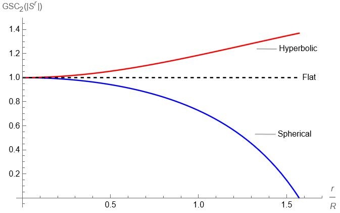
Figure 9: $\mathcal{GSC}_{2}(||\mathcal{S}_{p}^{r}||)$ for a D-Sphere of scalar curvature $\frac{D(D-1)}{R^{2}}$, a hyperbolic D-space of scalar curvature $\frac{D(1-D)}{R^{2}}$, and euclidean D-dimensional space.

Using this, one can compute exactly all the generalized curvature definitions

$$\mathcal{GSC}_{\mathcal{D}}(||\mathcal{S}_{p}^{r}||)=1+(D-1)\,(\frac{r}{R})\,\coth\left(\frac{r}{R}\right),$$ (37)

$$\mathcal{GSC}_{\mathcal{I}}(||\mathcal{S}_{p}^{r}||)=\frac{D\,\frac{r}{R}\,\cot\left(\frac{r}{R}\right)}{\sinh\left(\frac{r}{R}\right)\,{}_{2}F_{1}\left(\frac{1}{2},\frac{D}{2},\frac{2+D}{2},-\sinh^{2}\left(\frac{r}{R}\right)\right)},$$ (38)

$$\mathcal{GSC}_{1}(||\mathcal{S}_{p}^{r}||)=1+(D-1)\,(\frac{r}{R})\,(\coth\left(\frac{r}{R}\right)-(\frac{r}{R})\,\csch^{2}\left(\frac{r}{R}\right)),$$ (39)

$$\mathcal{GSC}_{2}(||\mathcal{S}_{p}^{r}||)=\frac{12\,(\frac{r}{R})^{2}\coth\left(\frac{r}{R}\right)}{-6(\frac{r}{R})^{2}-\pi^{2}+12\,(\frac{r}{R})\,\log\left(1-e^{2(\frac{r}{R})}\right)+6\text{PolyLog}_{2}\left(e^{2(\frac{r}{R})}\right)},$$ (40)

$$\mathcal{GSC}_{3}(||\mathcal{S}_{p}^{r}||)=\frac{\sqrt{\cosh^{2}\left(\frac{r}{R}\right)}\,{}_{2}F_{1}\left(\frac{1}{2},\frac{D}{2},\frac{2+D}{2},-\sinh^{2}\left(\frac{r}{R}\right)\right)\left((D-1)+(\frac{r}{R})^{-1}\,\tanh\left(\frac{r}{R}\right)\right)}{D},$$ (41)

$$\mathcal{GSC}_{4}(||\mathcal{S}_{p}^{r}||)=\frac{1}{D\sinh^{D+1}\left(\frac{r}{R}\right)}\Big{[}\left((\int_{0}^{(\frac{r}{R})}\frac{\sinh^{D-1}\left(y\right)}{y}\,dy)\sinh^{2}\left(\frac{r}{R}\right)+\sinh^{D+1}\left(\frac{r}{R}\right)\right)\\ \times\left(D-(\frac{r}{R})^{-1}\,\sqrt{\cosh^{2}\left(\frac{r}{R}\right)}\,{}_{2}F_{1}\left(\frac{1}{2},\frac{D}{2},\frac{2+D}{2},-\sinh^{2}\left(\frac{r}{R}\right)\right)\tanh\left(\frac{r}{R}\right)\right)\Big{]},$$ (42)

$$\mathcal{GSC}_{5}(||\mathcal{S}_{p}^{r}||)=1+\frac{(D-1)^{2}}{12}(\frac{r}{R})\csch^{2}\left(\frac{r}{R}\right)\Big{[}6(\frac{r}{R})^{2}+\pi^{2}+6(\frac{r}{R})(1-2i\pi)+6(\frac{r}{R})\cosh\left(\frac{2r}{R}\right)\\ -12(\frac{r}{R})\log(-1+e^{\frac{2r}{R}})-6\text{PolyLog}_{2}\left(e^{2(\frac{r}{R})}\right)\Big{]},$$ (43)

where $\int_{0}^{\frac{r}{R}}\frac{\sinh^{D-1}\left(y\right)}{y}\,dy$ was kept in integral form, but can be computed exactly for any $D\geq 2$.

One can see that $\mathcal{GSC}_{2}(||\mathcal{S}_{p}^{r}||)$ is independent of the dimension of the underlying space, for both positive and negative constantly curved spaces. This renders $\mathcal{GSC}_{2}(||\mathcal{S}_{p}^{r}||)$ ideal for making comparisons of $\mathcal{GSC}_{i}$ of general spaces. For the sake of completeness, we include a plot for $\mathcal{GSC}_{2}(||\mathcal{S}_{p}^{r}||)$ as a function of $\frac{r}{R}$ in Fig. 9.

References

- [1] R Loll, G Fabiano, D Frattulillo and F Wagner “Quantum gravity in 30 questions” In arXiv preprint arXiv:2206.06762, 2022
- [2] R Loll “Quantum gravity from causal dynamical triangulations: a review” In Classical and Quantum Gravity 37.1 IOP Publishing, 2019, pp. 013002 arXiv:1905.08669
- [3] R. Loll “Quantum Curvature as Key to the Quantum Universe”, 2023 arXiv:2306.13782 [gr-qc]
- [4] T. Regge “General relativity without coordinates” In Il Nuovo Cimento (1955-1965) 19.3, 1961, pp. 558–571 DOI: 10.1007/BF02733251
- [5] Yann Ollivier “Ricci curvature of Markov chains on metric spaces” In Journal of Functional Analysis 256.3, 2009, pp. 810–864 DOI: https://doi.org/10.1016/j.jfa.2008.11.001
- [6] N. Klitgaard and R. Loll “Introducing quantum Ricci curvature” In Physical Review D 97.4 American Physical Society (APS), 2018 DOI: 10.1103/physrevd.97.046008
- [7] R. Loll “Quantum Curvature as Key to the Quantum Universe” In arXiv e-prints, 2023, pp. arXiv:2306.13782 DOI: 10.48550/arXiv.2306.13782
- [8] Karl-Theodor Sturm “On the geometry of metric measure spaces” In Acta Mathematica 196.1 Institut Mittag-Leffler, 2006, pp. 65–131 DOI: 10.1007/s11511-006-0002-8
- [9] Alfred Gray “The volume of a small geodesic ball of a Riemannian manifold.” In Michigan Mathematical Journal 20.4 University of Michigan, Department of Mathematics, 1974, pp. 329–344
- [10] Alexander Grigor’yan, Jiaxin Hu and Ka-Sing Lau “Heat Kernels on Metric Measure Spaces” In Geometry and Analysis of Fractals Berlin, Heidelberg: Springer Berlin Heidelberg, 2014, pp. 147–207
- [11] Gregory F Lawler “Random walk and the heat equation” American Mathematical Soc., 2010
- [12] Dmitri V Vassilevich “Heat kernel expansion: user’s manual” In Physics reports 388.5-6 Elsevier, 2003, pp. 279–360
- [13] N. Klitgaard and R. Loll “Implementing quantum Ricci curvature” In Physical Review D 97.10 American Physical Society (APS), 2018 DOI: 10.1103/physrevd.97.106017
- [14] Der-Tsai Lee and Bruce J Schachter “Two algorithms for constructing a Delaunay triangulation” In International Journal of Computer & Information Sciences 9.3 Springer, 1980, pp. 219–242
- [15] Tong Wang “Poisson-Disk Sampling: Theory and Applications” In Encyclopedia of Computer Graphics and Games Cham: Springer International Publishing, 2020, pp. 1–8 DOI: 10.1007/978-3-319-08234-9_398-1
- [16] J. Ambjørn, J. Jurkiewicz and Y. Watabiki “On the fractal structure of two-dimensional quantum gravity” In Nuclear Physics B 454.1-2 Elsevier BV, 1995, pp. 313–342 arXiv:hep-lat/9507014
- [17] Jan Ambjørn, Andrzej Görlich, Jerzy Jurkiewicz and Renate Loll “Quantum gravity via causal dynamical triangulations” In Springer handbook of spacetime Springer, 2014, pp. 723–741
- [18] Jan Ambjørn, Lisa Glaser, Yuki Sato and Yoshiyuki Watabiki “2d CDT is 2d Hořava–Lifshitz quantum gravity” In Physics Letters B 722.1-3 Elsevier, 2013, pp. 172–175
- [19] J. Ambjørn, A. Görlich, J. Jurkiewicz and R. Loll “Nonperturbative quantum gravity” In Physics Reports 519.4-5 Elsevier BV, 2012, pp. 127–210 DOI: 10.1016/j.physrep.2012.03.007
- [20] Jesse Duin “Curvature correlations in Quantum Gravity” To appear, 2023 URL: https://www.ru.nl/highenergyphysics/theses/master-theses/
- [21] J. Ambjørn, K.. Anagnostopoulos and R. Loll “New perspective on matter coupling in 2D quantum gravity” In Physical Review D 60.10 American Physical Society (APS), 1999 arXiv:hep-th/9904012
- [22] J. Ambjørn, K. Anagnostopoulos and R. Loll “Crossing the c=1 barrier in 2D Lorentzian quantum gravity” In Physical Review D 61.4 American Physical Society (APS), 2000 arXiv:hep-lat/9909129
- [23] J. Brunekreef and R. Loll “Quantum flatness in two-dimensional quantum gravity” In Physical Review D 104.12 American Physical Society (APS), 2021 DOI: 10.1103/physrevd.104.126024