What can we learn from diffusion about Anderson localization
of a degenerate Fermi gas?

Abstract

Disorder can fundamentally modify the transport properties of a system. A striking example is Anderson localization, suppressing transport due to destructive interference of propagation paths. In inhomogeneous many-body systems, not all particles are localized for finite-strength disorder, and the system can become partially diffusive. Unravelling the intricate signatures of localization from such observed diffusion is a long-standing problem. Here, we experimentally study a degenerate, spin-polarized Fermi gas in a disorder potential formed by an optical speckle pattern. We record the diffusion in the disordered potential upon release from an external confining potential. We compare different methods to analyze the resulting density distributions, including a new method to capture particle dynamics by evaluating absorption-image statistics. Using standard observables, such as diffusion exponent and coefficient, localized fraction, or localization length, we find that some show signatures for a transition to localization above a critical disorder strength, while others show a smooth crossover to a modified diffusion regime. In laterally displaced disorder, we spatially resolve different transport regimes simultaneously which allows us to extract the subdiffusion exponent expected for weak localization. Our work emphasizes that the transition toward localization can be investigated by closely analyzing the system’s diffusion, offering ways of revealing localization effects beyond the signature of exponentially decaying density distribution.

I Introduction

In 1958, P. W. Anderson showed that a single electron in a disordered material will show an absence of diffusion at long times, i.e., it localizes [1, 2]. The tails of the particle’s wave function or probability density profile decay exponentially in space $\langle n(r)\rangle\sim\mathrm{exp}(-|r|/\xi)$, where $n$ is the particle density, $r$ is the position, $\xi$ is the localization length, and $\langle\cdot\rangle$ is a disorder and quantum average. In one and two dimensions, localization in random potentials always emerges from a particle interfering with its multiple scattering paths. This interference is constructive only at the spatial point where the particle has been initially placed. In $d=3$ dimensions, the system becomes critical, as not all scattering paths are expected to return to the origin. Thus, localization is expected only if the disorder becomes sufficiently strong [2]. In this case, a metal-insulator transition is expected with power law divergence at a critical value $\xi(E)\sim|E-E_{c}|^{-\nu}$ where $E$ is the energy, $E_{c}$ is a critical energy called “mobility edge”, and $\nu\approx$1.58\text{\,}$$ is the critical exponent [3, 4, 5]. Within the last 65 years, such Anderson localization (AL) [1, 2] has been observed in non-interacting systems of light [6, 7, 8, 9, 10], ultrasound [11, 12, 13], and microwaves [14, 15]. In the context of ultracold atoms, AL has been intensively studied in 1D, both in the quasiperiodic lattice [16] and in the continuum [17], in 2D [18, 19, 20], as well as in 3D [21, 22, 23].

During the last years, the investigation of the Anderson metal-insulator transition has increased significantly [24, 25, 26] due to an active debate whether an interacting system is able to localize at a finite disorder strength [27, 28, 29, 30, 31, 32, 33, 34, 35, 36]. Moreover, even in the non-interacting case, the literature seems not fully conclusive as the most striking feature, the exponential tails of Anderson-localized particles, can simply be an artefact from an energy-dependent diffusion coefficient $D(E)$ [37, 38, 39]. In particular, this is a problem for fermionic systems, where a broad distribution of $D(E)$ due to Pauli exclusion is present. Since the observation of an exponential decay of the wavefunction as a smoking gun for AL is not sufficient, other signatures for localization from experimentally accessible observables are required.

Experimentally, a common technique to study transport phenomena is via a quantum quench [17, 16, 40, 22, 21]. Here, an initial equilibrium state is prepared in a harmonic trap, usually at a low temperature, and then quenched into a disorder potential while simultaneously extinguishing the trap. Classically, one expects the particles to undergo standard Brownian diffusion when expanding through such a disordered potential landscape. Due to quantum interference effects leading to localization, however, anomalous subdiffusion is expected for particles close to the mobility edge [41, 38] while the diffusion coefficient approaches the Heisenberg-limited ratio of the reduced Planck constant and the particle mass, the “quantum of diffusion” $\hbar/m$ [42, 22, 23, 39, 38, 43, 44, 45]. Hence, the evolution of a system toward localization can be investigated by closely observing its diffusion.

Generally, different regimes of anomalous diffusion are distinguished by the exponent $\alpha$ of the growing mean squared displacement (MSD) of a particle from its initial position $r(t=0)$,

$$\mathrm{MSD}(r(t))\equiv\langle|r(t)-r(0)|^{2}\rangle=2dD_{\alpha}t^{\alpha},$$ (1)

which evolves over time $t$ and anomalous diffusion coefficient $D_{\alpha}$ [46, 47, 48, 49]. For $\alpha=1$, the system undergoes normal diffusion, subdiffusion for $\alpha<1$ and superdiffusion for $\alpha>1$. Another special case, $\alpha=2$, is called ballistic diffusion and describes the free expansion without any medium, while also occurring in non-trivial cases [48, 50, 46].

Here, we study the expansion of a non-interacting Fermi gas into a disordered optical waveguide. Recording the dynamics of the density distribution upon releasing the system from the trap allows us to observe the diffusive expansion and deviations from normal diffusion which we attribute to signatures of Anderson localization. We compare different methods to obtain anomalous-diffusion observables, i.e., exponent and coefficient, from absorption images taken, and we analyze them for signatures for localization.

II Experimental methods

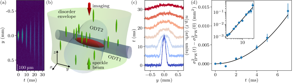
Figure 1: Schematic illustration of the experimental setup, absorption images and evaluation of disorder-free ballistic expansion. (a) Absorption images taken at various expansion durations $t$. 50 repetitions have been averaged per image. (b) Experimental setup. The atomic cloud (red ellipsoid) is initially trapped in a superposition of two optical dipole traps (blue tubes). The speckle beam (green volume and arrow), propagating along the $+z$ axis, produces randomly distributed anisotropic grains (green ellipsoids). At $t=0$, the crossed dipole trap is extinguished and the atoms begin to expand along the $y$ axis. The cloud is imaged after a variable expansion duration $t$ with a resonant beam (red arrow) which propagates along the $-z$ direction. (c) Density profiles $n(y,t)$ for equidistant time steps (bottom to top, left axis). The profiles have been calculated from the absorption images shown in (a) by integrating along the $x$ axis. (d) Variance $\sigma^{2}_{\mathrm{IPW}}(t)-\sigma^{2}_{\mathrm{IPW}}(0)$ over time for short timescales, the solid line is a power-law fit with exponent $\alpha=2.02\,\pm\,0.09$, see Eq. (2). Error bars are calculated from error propagation. In the inset, the same fit with more data for longer timescales is shown in a double-logarithmic plot.

Experimentally, we prepare a degenerate Fermi gas of typically $N=10^{5}$ ⁶Li atoms, polarized in the lowest-lying Zeeman substate and inside a crossed optical dipole trap (see Fig. 1(b)). Due to the fermionic nature of the atoms, for the low temperature $T\approx$100\text{\,}\mathrm{n}\mathrm{K}$\approx$0.15\text{\,}$\,T_{\mathrm{F}}$ (with Fermi temperature $T_{\mathrm{F}}$) of the atomic samples, $s$-wave interactions are prohibited, while $p$-wave and higher order interactions are strongly suppressed. Hence, in good approximation, the atomic cloud behaves as an ideal Fermi gas [51, 38, 52]. Initially, the atoms are trapped in an optical dipole trap (ODT), created by superposing a focused laser beam ODT1, propagating along the $y$ axis, with a secondary beam ODT2, crossing the first laser beam at an angle of 53° in the $x$-$y$ plane, see Fig. 1(b). The resulting crossed trap has the trap frequencies $(\omega_{x}^{\times},\omega_{y}^{\times},\omega_{z}^{\times})=(386,37.8,257)\times 2\pi\,$\text{\,}\mathrm{H}\mathrm{z}$$, with the superscript $\times$ denoting the crossed trap. By extinguishing ODT2 at $t=0$, the trap frequencies become $(\omega_{x},\omega_{y},\omega_{z})=(365,1.9,248)\times 2\pi\,$\text{\,}\mathrm{H}\mathrm{z}$$. This happens instantaneously, i.e. at a duration smaller than $1\text{\,}\mathrm{\SIUnitSymbolMicro s}$ much shorter than the inverse trap frequency. The trap geometry along the $x$ and $z$ axis does not change significantly, $\omega_{x,z}\approx\omega_{x,z}^{\times}$, while the potential along the $y$ axis effectively becomes flat, $\omega_{y}\ll\omega_{y}^{\times}$, allowing the atoms to expand along the $y$ direction. After a variable expansion duration $t$, we perform resonant high-intensity absorption imaging [53, 54, 55] along the $z$ axis.

To probe diffusion in disorder, a repulsive optical speckle disorder potential $V(x,y,z)$ composed of $532\text{\,}\mathrm{nm}$ laser light and with a typical grain size $\eta_{x,y}^{2}\times\eta_{z}=($750\text{\,}\mathrm{nm}$)^{2}\times$10.2\text{\,}\mathrm{\SIUnitSymbolMicro m}$$ is quenched on at $t=0$, where $\eta_{x,y}$ and $\eta_{z}$ are the correlation lengths along the respective directions [55, 56, 42]. We note that this three-dimensional speckle potential does not allow for classically bound states [57, 58, 59]. We characterize the disorder strength by its spatial average $\langle V\rangle$. In this work, we investigate the effect of disorder strengths of up to $\langle V\rangle\approx$700\text{\,}\mathrm{n}\mathrm{K}$\times k_{\mathrm{B}}$, which can be somewhat larger than the typical Fermi energies $E_{\mathrm{F}}\approx$600\text{\,}\mathrm{n}\mathrm{K}$\times k_{\mathrm{B}}$.

For all settings, i.e. expansion duration and disorder strength, we create and image 50 realizations of the atom sample and rotate the speckle diffusor plate in between slightly to create a unique disorder realization for each shot. These images are averaged to ensure a good disorder average [38] and to reduce the impact of noise in the evaluation. For this setup in particular, image noise is enhanced due to technical details (see Appendix A) compared to our previous works, requiring more averaging for the same signal-to-noise ratio. To analyze the expansion along the $y$ direction, we integrate the averaged images taken at time $t$ over the $x$ axis, see Fig. 1(a) and (c). This yields the column densities $n(y,t)$ for the one-dimensional density distributions we analyze as described in Sec. III.

Finally, we use $d=1$ in the diffusion analysis as the dimensions $x,z$ are blocked from undergoing diffusion due to the harmonic confinement or, in other words, $D_{x,z}=0$. However, we emphasize that the gas as well as the speckle disorder never cross into the regimes of dimensionality lower than $d=3$.

III Diffusion observables

In non-interacting systems, we expect particles to diffuse ballistically, normally or anomalously (subdiffusively [38]) when the system is either subjected to no disorder, weak disorder or strong disorder, respectively. Ideally, diffusion is investigated by evaluating the mean squared displacement computed from trajectories of single particles traced over time [60, 46]. Since we, like the majority of cold-gas experiments, cannot physically access the individual-trajectory MSD as defined in Eq. (1), we need to restrict ourselves to observables characterizing the ensemble of many particles. In this section, we look at four different observables of the spatial variance $\sigma^{2}_{i}$ of the cloud that we briefly introduce and then compare each to their ability to extract the diffusion exponent $\alpha$ as well as coefficient $D_{\alpha}$ from

$$\sigma_{i}^{2}(t)-\sigma_{i}^{2}(0)=2D_{\alpha}t^{\alpha}.$$ (2)

Here $i$ stands for the different methods to extract the variance,

1. $\sigma_{\mathrm{fit}}^{2}$, the variance of a Gaussian fitted to the density profile, see Sec. III.1,

2. $\sigma_{\mathrm{Var}}^{2}$, the spatial variance of the density profile, see Sec. III.2,

3. $\sigma_{\mathrm{PR}}^{2}$, the variance extracted from the participation ratio (PR), see Sec. III.3, and

4. $\sigma_{\mathrm{IPW}}^{2}$, the variance extracted from the inverse participation width (IPW), see Sec. III.4.

To find an appropriate estimate for the spatial variances of the cloud, we use a Gaussian function

$$n_{\mathrm{Gauss}}(y,y_{0},t)=\frac{N(t)}{\sqrt{2\pi\sigma^{2}(t)}}\mathrm{exp}\left(-\frac{(y-y_{0})^{2}}{2\sigma^{2}(t)}\right)$$ (3)

as a control distribution representing the density profile of the experimental data (see Fig. 1(c)), with atom number $N(t)=\sum_{y}n(y,t)\Delta y$, density $n(y,t)$ on position $y$ and $\Delta y$ the size of a pixel. Note that we fix $y_{0}=0$ in the following. Here, the variance is time-dependent, following Eq. (2) with $\alpha=2$ for ballistic, $\alpha=1$ for normal, and $\alpha<1$ for anomalous subdiffusion, respectively.

The accurate determination of the diffusion exponent remains an actively investigated topic [46]. For the present work, we chose the following procedure. By taking the logarithm of Eq. (2),

$$\ln\left(\sigma_{i}^{2}(t)-\sigma_{i}^{2}(0)\right)=\ln\left(2D_{\alpha}t^{\alpha}\right)=\ln{\left(2D_{\alpha}\right)}+\alpha\ln t,$$ (4)

the diffusion exponent $\alpha$ can be directly inferred via linear regression. We use the standard fit error as uncertainty of the exponent’s error. An example of this fit to $\sigma_{\mathrm{IPW}}^{2}(t)-\sigma_{\mathrm{IPW}}^{2}(0)$ as extracted from data from a ballistic expansion without disorder, which is discussed in more detail in Sec. III.5, is shown in Fig. 1(d). For the anomalous diffusion coefficient, we calculate

$$D_{\alpha}=\left\langle\frac{\sigma_{i}^{2}(t)-\sigma_{i}^{2}(0)}{2t^{\alpha}}\right\rangle.$$ (5)

Note that the set of values for different $t$ that are averaged is constant in time. For the error of $D_{\alpha}$, we use the standard deviation of that set. Even though $D_{\alpha}$ is already contained in the fit result as the variance-axis intercept, we decide for this option to be less dependent on fit results. Note that both options yield values that are equal within their ranges of uncertainties.

Comparing the anomalous diffusion coefficient $D_{\alpha}$ for different $\alpha$ is not straightforward. Technically, it has the unit of $\mathrm{m}^{2}\,\mathrm{s}^{-\alpha}$, or normalized to the diffusion quantum $\hbar/m$ as $mD_{\alpha}/\hbar$, the unit of $\mathrm{s}^{1-\alpha}$ [47]. The alternative method is to remove the dependence on $\alpha$ by focusing on $D_{1}(t)=D_{\alpha}t^{\alpha-1}$ which has the unit of $\text{\,}{\mathrm{m}}^{2}\text{\,}{\mathrm{s}}^{-1}$. However, $D_{1}(t)$ will then not be a constant in time for $\alpha\neq 1$, making a direct comparison of single representative values of the diffusion coefficient for different settings with different $\alpha$ not possible. Hence, we decide to evaluate $D_{\alpha}$ as described.

III.1 Gauss-fit variance

One of the most simple and also most common methods is to fit a distribution function to the recorded density profiles [40, 16, 61, 62], see Fig. 2 (a), and extract values such as the variance or peak height. On the one hand, fitting has the advantage of approximating the raw data without any other forms of data filtering and averaging. On the other hand, the results strongly depend on the fitting function and number of fit parameters. In particular, the number of fit parameters needs to be restricted to as few parameters as possible to avoid overfitting and therefore omitting the general properties of the dynamics [63, 64]. In the case of normal diffusion, fitting Eq. (3) becomes straightforward. The variance $\sigma_{\mathrm{fit}}^{2}$ is then directly extracted from the fitted parameters. As the density profile consists of about $10^{5}$ fermions, one would naively expect the central-limit theorem to be valid. This is, however, only the case when the diffusion coefficient is not energy dependent. Since this is generally not the case in our experiment, deviations from the Gaussian density distribution will be present in the profiles, which we discuss in more detail in Appendix D. Still, a Gaussian fit is a good approximate for the first and second moment $\sigma^{2}(t)$ of the true density profile, and thus sufficient to extract the diffusion exponent and coefficient.

III.2 Variance of the density profile

Another common and more direct method is to compute the mean squared displacement of the distribution [22]

$$\sigma_{\mathrm{Var}}^{2}(t)\coloneqq\frac{1}{N(t)}\sum_{y}n(y,t)\,(y-y_{\mathrm{com}})^{2}\Delta y,$$ (6)

with the center-of-mass position $y_{\mathrm{com}}$. As $y_{\mathrm{com}}$, we choose the cloud-peak position taken from fitting the Gaussian since it is significantly more stable against noise when compared to calculating the center-of-mass position directly as the mean of the distribution. Similarly, we need to omit negative $n(y,t)$ arising from our imaging system, which is calibrated to $\langle n\rangle=0$ if no atoms are present.

III.3 Participation ratio

As a complementary approach, we present the participation ratio (PR) [65, 66, 9, 67, 68]

$$\mathrm{PR}(t)=\frac{\left(\sum_{y}n(y,t)\Delta y\right)^{2}}{\sum_{y}n^{2}(y,t)\Delta y}.$$ (7)

Note that PR$(t)$ has the physical dimension of length here, describing the cloud width here. Here, the inverse PR is proportional to the probability of a particle returning to the same position after infinite time [69]. Similarly, the cloud’s displacement becomes $\mathrm{PR}(t)^{2}\sim D_{\alpha}t^{\alpha}$, and in the perfectly localized case in the continuum is expected to follow $\mathrm{PR}=4\xi$ [68]. Although not commonly used to investigate diffusion, we expect PR to be constrained by upper bounds of particle transport [70]. To estimate the variance, we evaluate PR for the Gaussian control distribution, Eq. (3),

$$\sigma_{\mathrm{PR}}^{2}(t)\coloneqq\frac{\mathrm{PR}^{2}(t)}{4\pi}.$$ (8)

This quantity tends to underestimate the diffusion exponent and coefficient.

III.4 Inverse participation width

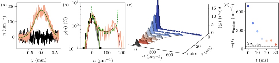
Figure 2: Density-histogram analysis. (a) Noisy line-density plot (orange line) as calculated from absorption image and its Gauss fit (dark-green dashed line) as well as line density from noise measurement (black line). Here, data from the disorder-free expansion at $t=$20\text{\,}\mathrm{ms}$$ are shown as a representative example. (b) Histograms of the data shown in panel (a), with same line colors and types. Additionally, the noise histogram is fitted with a normal distribution (light-green dash-dotted line). Further, the convolution of the fit-function histogram with the noise Gauss-fit is plotted (red dash-dotted line) to visualize the convolution character of histograms. (c) Evolution of histograms over time, shown as bar plots for the same set of data as shown in Fig. 1. The noise histogram is additionally plotted at the front in black (labeled “noise”). The black dashed line below the decreasing histogram width is a guide to the eye. (d) Widhts $w(t)$ of all histograms shown in (c) over time, offset by noise-histogram width $w_{\mathrm{noise}}$. The dash-dotted line shows $2\sigma_{\mathrm{noise}}$ as the lower validity bound of IPW. Error bars are the standard deviation of the noise histogram.

Having access to local counting statistics [60, 71, 72, 73, 74, 75, 76, 77] allows to obtain fundamental indicators for general particle diffusion and localization. Extracting these statistics is, however, not feasible in experimental setups with large amounts of particles and high densities. Similarly, when considering the Gaussian camera noise, we would need thousands of realizations to build a significant statistic. Instead of focusing on particle statistics, complementary approaches have evaluated the intensity contrast of the measured image [78] as an indicator of (de)localization. Similarly, we decided to investigate the image histograms, which correspond to the distribution of particle densities recorded in an absorption image. By inspecting the normalized ordinary histogram $p(n,t)$, and the underlying distribution of densities, we gain additional knowledge to extract the diffusion details.

We calculate $p(n,t)$ from the line density $n(y,t)$ by counting the number of densities that fall into 100 bins between the smallest and largest density recorded at time $t$. We normalize $\sum_{n}p(n,t)=1$, such that $p(n,t)$ corresponds to a discrete probability density function (PDF) of the occurrences of densities $n$. Examples of density distributions and their histograms are shown in Fig. 2(a, b), where we discuss the different cases in more detail below.

Here, we introduce a noise-robust method to extract the peak density which we call the “inverse participation width” (IPW), a quantity based on the width of these histograms. From IPW, we extract $\sigma^{2}_{\mathrm{IPW}}$ and, thus, the diffusion exponent and coefficient. The histograms provide criteria for when IPW is a good quantity to extract the diffusion details and give an insight how noise and IPW are related, which we discuss later in this paragraph. To get a more profound view on the image-histogram dynamics, we first discuss the histogram shapes as well as IPW itself for noise-free densities, then for the histogram-contribution of camera noise alone, and finally for the combined histograms as recorded in the experiment.

We begin with the noise-free case and a unimodal density distribution in space such as a Gaussian (see Eq. (3) and the green dashed line in Fig. 2(a)). Then, the image histogram $p(n,t)$ shows two effectively diverging flanks at $n=0$, no particles, and $n=n(y=0,t)=N(t)/\sqrt{2\pi\sigma^{2}(t)}$ for the Gaussian function, corresponding to the peak density at time $t$ (see green dashed line in Fig. 2(b)). Further, the kernel of the histogram, see appendix B, follows

$$p_{\mathrm{Gauss}}(n,t)\sim\frac{1}{n\sqrt{-\mathrm{ln}\left(\frac{n\sqrt{2\pi\sigma^{2}(t)}}{N(t)}\right)}}$$ (9)

for $0<n<n(0,t)$, the support of the kernel, which is given by the peak amplitude $n(0,t)$ of the distribution. This means that the full width $w(t)\coloneqq n_{\mathrm{max}}(t)-n_{\mathrm{min}}(t)$ of the histogram is equal to the peak density $n(0,t)$. This holds true for any unimodal distribution in space. From the peak density, we can extract the Gauss variance directly as $\sigma^{2}(t)=N^{2}(t)/(2\pi w^{2}(t))$. Note that this relation for $\sigma$ only holds true in the noise-free case. The variance we extract from the experimental data, in which noise plays a significant part, is discussed further below. We consider IPW a good observable to extract $\sigma(t)$ as long as the noise-free profile of $p(n,t)$ is effectively diverging at the flanks, meaning that the decreasing width $w(t)$ captures the most relevant part of the distribution change. Like the other diffusion observables, IPW is not sensitive to the tails of spatial distributions.

In the second case, we focus on the camera noise by itself. Experimentally, we expect noise in absorption images to result from spatial and temporal atom-number or imaging-beam-intensity fluctuations, random influences by stray light or similar factors, as well as camera noise, including shot noise, thermal or electronic fluctuations. To investigate the noise that is present in the absorption images, we conduct the experimental sequence without the sample and take the average from 50 images with only noise. We calculate the histogram $p_{\mathrm{noise}}$ of the averaged image and fit it with a Gaussian function $p^{\mathrm{fit}}_{\mathrm{noise}}$, see light-green dotted line in Fig. 2(b), which we find to agree very well with the noise histogram. Finally, we compute the width $w_{\mathrm{noise}}$ of the histogram and use the standard deviation $\sigma_{\mathrm{noise}}$ from the fit as the statistical uncertainty for $w$ and $n$.

In the third case, we consider the histogram $p_{\mathrm{data}}$ of the noisy density distribution and, hence, the experimentally relevant case. With noise, the density distribution fluctuates, yielding a wider histogram as $n<0$ and $n>n(0,t)$ will be observed as well. In fact, as is expected for the probability density function of the sum of two random variables, the combined histogram $p_{\mathrm{data}}$ of signal $p$ and noise $p_{\mathrm{noise}}$ is given by the convolution

$$p_{\mathrm{data}}(n,t)=(p_{\mathrm{noise}}*p)(n)=\sum_{n^{\prime}=-\infty}^{\infty}p_{\mathrm{noise}}(n^{\prime})p(n-n^{\prime},t),$$ (10)

see the orange solid line for the data histogram $p_{\mathrm{data}}$ as well as the red dash-dotted line for $p^{\mathrm{fit}}_{\mathrm{noise}}*p_{\mathrm{Gauss}}$ in Fig. 2(a). The resulting distribution is still bimodal, where the peaks are approximately located at the effectively diverging flanks of the noiseless distribution, e.g. $p(n,t)=p_{\mathrm{Gauss}}(n,t)$. Thus, for $w(t)-w_{\mathrm{noise}}>2\sigma_{\mathrm{noise}}$, the resulting histogram will be bimodal [79], see Fig. 2(c, d).

As the convolution near the diverging flanks resembles the convolution kernel, and hence the noise histogram $p_{\mathrm{noise}}$, we can approximate the noise-free peak density simply by $n(0,t)\approx w(t)-w_{\mathrm{noise}}$. With that, we define the noise-corrected inverse participation width as

$$\mathrm{IPW}(t)\coloneqq\frac{N(t)}{w(t)-w_{\mathrm{noise}}}$$ (11)

and the resulting observable for the variance is then

$$\sigma^{2}_{\mathrm{IPW}}(t)\coloneqq\frac{1}{2\pi}\mathrm{IPW}^{2}(t).$$ (12)

Note that the diffusion exponent $\alpha$ can be inferred from IPW${}^{2}(t)$ directly without any specific assumptions about the density profile except for its spatial unimodality.

We note that IPW in itself does not require any calculation of the histogram $p(n,t)$, as the width $w(t)$ can be extracted directly from the image. Since the validity and properties of IPW are derived directly from the image histograms and the underlying statistics, we chose to motivate the observable with the histogram analysis. We further state that the noise correction is intrinsic in the sense that the statistical properties of both the data and the system are exploited to reduce the effects of noise rather than trying to remove the noise from the data itself. For all other observables, noise reduction methods such as smoothing or wavelet decomposition are applied directly to the absorption images, significantly affecting them and potentially the extracted result.

Finally, we note that our efforts to solve the deconvolution problem of extracting $p$ from Eq. (10) have not produced satisfactory results for the experimental data. However, the application of machine learning to this problem could be a good prospect that we will explore in a future work.

III.5 Comparison of observable performance

Figure 3: Comparison of observable performance. Shown are the values for $\sigma_{i}^{2}(t)-\sigma_{i}^{2}(0)$ in a double-logarithmic plot (a, b) as well as the extracted diffusion exponent (c) and coefficient (d) for the Gauss-fit variance “fit” (orange triangles), profile variance “Var” (red squares), and width from the participation ratio PR (purple hexagons), and from IPW (green circles). (a) Ballistic expansion without disorder, $\langle V\rangle=$0\text{\,}\mathrm{n}\mathrm{K}$\times k_{\mathrm{B}}$. The black dashed line is Eq. (2) with fixed $\alpha=2$ and $D_{2}=\sigma^{2}\!(0)\omega_{y}^{2}/2$. Points plotted in lighter colors were omitted from the fitting procedure. Gauss-fit-variance error bars are standard errors from the fit while errors of Var, PR, and IPW are calculated from error propagation. (b) Expansion in weak disorder, $\langle V\rangle=$160\text{\,}\mathrm{n}\mathrm{K}$\times k_{\mathrm{B}}$, with point colors and symbols as in panel (a). Note that the vertical light-green line is the error bar of the final value of $\sigma_{\mathrm{IPW}}^{2}(t)$. The black dotted line is Eq. (2) with fixed $\alpha=1$ and $D_{1}=10\hbar/m$. Note that the value of $D_{1}$ is not the expectation for this data set and is chosen to yield a guide to the eye, see Sec. III.5. (c) Diffusion exponent $\alpha$ as extracted from fits to the data shown in (a, data on top) and (b, data on the bottom). The expectation for the ballistic exponent $\alpha=2$ (normal-diffusion exponent $\alpha=1$) is plotted as a dashed (dotted) line. Areas shaded in gray show results of a numerical investigation of observable performance (see Appendix C for details). Error bars are standard errors from fit. (d) Diffusion coefficient $D_{\alpha}$. Error bars are standard deviations of values used to calculate $D_{\alpha}$ (see Eq. (5)) and are too small to be seen.

In order to choose the best observable for our system, we focus on the evaluation of two representative data sets, where the first data set correspond to ballistic and the second to normal diffusion. We compare the extracted diffusion exponent $\alpha$ and generalized coefficient $D_{\alpha}$ from the respective observable with expectations for both data sets.

For the first data set, see Fig. 3(a), the disorder was absent ($\langle V\rangle=0$). Here, we predict a free expansion (ballistic diffusion) with $\alpha=2$ and $D_{2}=\sigma^{2}\!(0)\omega_{y}^{2}/2\eqqcolon v_{\mathrm{pr.}}^{2}$ (dashed line). The latter is the square velocity along the $y$ axis for a non-interacting gas released from a harmonic trap [80]. We use $\sigma(0)=$53\text{\,}\mathrm{\SIUnitSymbolMicro m}$$ from a Gauss fit to the trapped cloud to get $v_{\mathrm{pr.}}\approx$8.9\text{\,}\mathrm{mm}\text{\,}{\mathrm{s}}^{-1}$$. As can be seen in Fig. 3(a), the different observables are all generally in line with the expectation.

For the second data set, shown in Fig. 3(b), weak disorder $\langle V\rangle=$160\text{\,}\mathrm{n}\mathrm{K}$\times k_{\mathrm{B}}\approx E_{\mathrm{F}}/4$ was applied to investigate diffusive expansion. Similarly to before, all observables generally follow the linear normal-diffusion behavior (dotted line) with $\alpha=1$. Note that $\alpha=1$ is only our expectation for this data set, as it is, to our knowledge, not possible to objectively infer a priori which exact type of diffusion occurs at these weak disorder strengths. Still, we chose this data set, because, for even smaller disorder strength, finite-size effects could effectively increase $\alpha$, as is described in more detail in Sec. IV.1. The diffusion coefficient $D_{1}=10\hbar/m$, used for the dotted line in Fig. 3 (b), is set to yield a guide to the eye. As stated above, we aim to make the distinction between normal diffusion and subdiffusion (for stronger disorder). Correspondingly, we consider the determination of $\alpha=2$ to be the more important benchmark for the observables.

We show the performances of the observables in determining the diffusion exponent and coefficient, see Fig. 3(c) and (d), respectively. Furthermore, for the exponent $\alpha$, we present the results of a numerical investigation indicated by gray areas. More specifically, we generated numerical data of a noisy Gaussian function whose width increased according to Eq. (2) either ballistically ($\alpha=2$) or diffusively ($\alpha=1$) and evaluated it identically to the measurement data. More details can be found in Appendix C. In the following, we focus on the performances of each observable separately.

The Gauss-fit variance $\sigma^{2}_{\mathrm{fit}}$ (Sec. III.1) captures the ballistic expansion very well but claims subdiffusion for the second data set. For the ballistic case, the velocity $\sqrt{D_{2,\mathrm{fit}}}\approx$9.7\text{\,}\mathrm{mm}\text{\,}{\mathrm{s}}^{-1}$$ we extract from the data set as described in Eq. (5) is the closest of all observables to the prediction $v_{\mathrm{pr.}}\approx$8.9\text{\,}\mathrm{mm}\text{\,}{\mathrm{s}}^{-1}$$. Importantly, $\sigma^{2}_{\mathrm{fit}}$ appears to saturate toward larger $t$ in Fig. 3(b), which could cause the lower exponent. A remaining curvature in a double-logarithmic plot signals a deviation from the modeled power-law behavior, meaning the analysis based on the anomalous diffusion as in Eq. (2) breaks down. As can be seen in Fig. 3(c), the numerically determined Gauss-fit variance expectedly yields very accurate exponents as the underlying distribution function is precisely the same, which is experimentally not the case. As stated in Ref. [38], the density profile of fermions diffusing through disorder is expected to differ quite significantly from a Gaussian function. The profile would be modified even further when localization is considered. As we discuss in more detail in Appendix D, it is not possible to discern the underlying shape due to the large noise present in the images. Using another function such as a generalized Gaussian would technically fit better to the data (see Appendix D) but its parameters might not yield as much physical meaning while possibly suffering from the mentioned problem of possible overfitting.

The exponent extracted from the variance of the density profile $\sigma^{2}_{\mathrm{Var}}$ (Sec. III.2) significantly underestimates the ballistic exponent for the first data set but is compatible to normal diffusion in the second one. In both cases, most of its initial values have to be omitted due to them being negative. Note that negative values are physically not sensible but arise due to too much noise influence if the observable does not increase significantly enough for earlier expansion times and, thus, subtracting $\sigma_{i}^{2}(0)$ can result in negative values. This susceptibility to noise is also reflected in the large uncertainties in the numerical analysis. The fact that $\sigma^{2}_{\mathrm{Var}}$ changes from strong fluctuations around the zero point to the interesting power law only for rather long expansion durations makes it problematic from the point of view of evaluation, as the signal of the data then approaches the magnitude of the camera noise (see Fig. 1(c) for example), which makes its prediction less reliable. We conclude that $\sigma^{2}_{\mathrm{Var}}$ is not a good observable for our system.

The participation ratio (Sec. III.3) has the obvious advantage that it is not dependent on external factors other than the atomic density detected. Moreover, it is quite robust against noise, at least compared to $\sigma^{2}_{\mathrm{Var}}$. According to the numerical investigation, $\sigma^{2}_{\mathrm{PR}}$ seems to be quite accurate in determining $\alpha$ for the case of normal diffusion, but it also finds a subdiffusive behavior for the experimental data. The major drawback, however, is the significant underestimation of the ballistic exponent for both the numerical and especially the experimental data set. Since it does not meet this benchmark, we cannot consider it a sufficiently good observable to accurately study anomalous diffusion in our system.

The statistical observable $\sigma^{2}_{\mathrm{IPW}}$ (Sec. III.4) agrees very well with the expectations in both cases. The numerical data suggests that it tends to generally overestimate both exponent and coefficient slightly while being quite precise especially for the case of normal diffusion. Indeed, the diffusion coefficient $D_{1}$ determined in the numerical investigation is consistently overestimated by a factor of less than two. For the coefficient determined for the ballistic case, we find $\sqrt{D_{2,\mathrm{IPW}}}\approx$12.3\text{\,}\mathrm{mm}\text{\,}{\mathrm{s}}^{-1}$$ which is slightly larger than $v_{\mathrm{pr.}}$. From that and since IPW yields the largest estimation for the diffusion coefficient of the investigated observables, the experimentally determined coefficient can be seen as a close upper bound. An additional property of $\sigma^{2}_{\mathrm{IPW}}$ is that, for very large timescales, the variance as well as its error begins to increase significantly. This occurs when $w(t)\approx w_{\mathrm{noise}}$, causing $\sigma^{2}_{\mathrm{IPW}}$ to diverge. This has the advantage that the choice of the fit range is quite obvious, see $\sigma^{2}_{\mathrm{IPW}}$ and its error bar for the largest $t$ in Fig. 3(b).

We conclude from the comparison that the Gaussian fit and IPW are both good observables. However, extracting the diffusion exponent would be done from a fit of fit results for $\sigma^{2}_{\mathrm{fit}}$, since we perform a linear regression as in Eq. (4). As the mentioned curvature of $\sigma^{2}_{\mathrm{fit}}$ is more strongly pronounced for expansions in stronger disorder, the precise choice of fit range would influence the final exponent significantly. In fact, this issue was the main motivation behind the search for alternative observables. Therefore, for the remainder of this work, we use the inverse participation width to determine the diffusion properties of the ultracold atom cloud.

IV Signatures of Anderson Localization

Using the inverse participation width, we analyze the behavior of the atoms when diffusing through disorder of different strength and infer signatures of Anderson localization from both deviations of normal diffusion and from additional quantities. We first focus on the diffusion and localization fraction when the full cloud is symmetrically diffusing in a disordered potential in Sec. IV.1. Second, we directly compare the spatially resolved probability density distributions of clouds diffusing in asymmetric disorder in Sec. IV.2. In this scenario, one part of the cloud diffuses into the disorder, while the other part shows close-to-ballistic diffusion in very shallow disorder.

IV.1 Diffusion in symmetric disorder

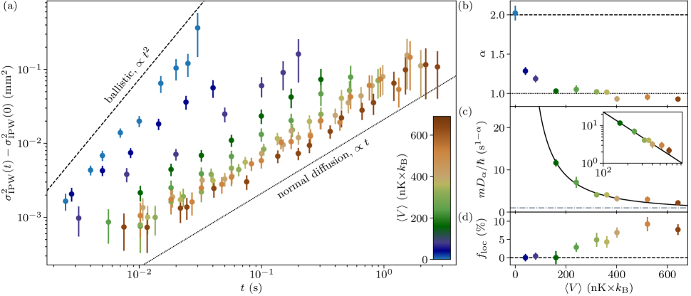
Figure 4: Expansion in disorder of variable strength. Without disorder (light blue on the upper left side), the atoms expand ballistically. For very weak disorder (dark blue), $\langle V\rangle<$100\text{\,}\mathrm{n}\mathrm{K}$\times k_{\mathrm{B}}$, the system appears to be super-diffusive due to finite-size effects. For weak to moderate disorder (green), $\langle V\rangle=$100400\text{\,}\mathrm{n}\mathrm{K}$\times k_{\mathrm{B}}$, the atoms undergo normal diffusion. For strong disorder (brown), $\langle V\rangle\geq$400\text{\,}\mathrm{n}\mathrm{K}$\times k_{\mathrm{B}}$, subdiffusion is observed. (a) Atom-cloud variance from IPW over time for different disorder strengths (colors), plotted double-logarithmically. Error bars are calculated from error propagation. The power laws for ballistic expansion (dashed line) and normal diffusion (dotted line) are plotted as a visual aid. (b) Diffusion exponent $\alpha$ over disorder strength. The dashed (dotted) line marks the ballistic-expansion (normal-diffusion) exponent. Error bars are standard errors from fit. (c) Diffusion coefficient $D_{\alpha}$ over disorder strength. Values of data with $\langle V\rangle<$100\text{\,}\mathrm{n}\mathrm{K}$\times k_{\mathrm{B}}$ were omitted to enhance visibility. The black line is a power-law fit which yields the exponent $-1.41\,\pm\,0.10$. The quantum of diffusion $\hbar/m$ is shown as a dash-dotted line. Error bars are standard deviations of values used to calculate $D_{\alpha}$. The inset shows same data as a double-logarithmic plot to highlight the power-law behavior of $D_{\alpha}$. (d) Fraction of localized atoms $f_{\mathrm{loc}}$ over disorder strength. Error bars are standard errors from fit.

Experimentally, we align the focus of the speckle-laser beam to the cloud position in order to ensure that the cloud can symmetrically diffuse along the $y$ axis in the disorder potential. From each disorder strength we take a series of in-situ absorption images for increasing diffusion time $t$ and extract the inverse participation width. An overview over the series of cloud variances for varying disorder strengths is shown in Fig. 4(a). All expansion series follow the expected power-law behavior (straight line in a double-logarithmic plot). For disorder strengths $\langle V\rangle>0$, the system quickly transitions from ballistic expansion towards normal diffusion. There is an apparent intermediate regime of $1<\alpha<2$ for $\langle V\rangle<$100\text{\,}\mathrm{n}\mathrm{K}$\times k_{\mathrm{B}}$ (dark-blue points) which can be explained by finite-size effects. Faster atoms with energies close to the Fermi energy $E_{\mathrm{F}}\gg\langle V\rangle$ perceive the disorder potential only as a small perturbation and can thus move approximately ballistically. Further, since the speckle-beam waist is finite at roughly $450\text{\,}\mathrm{\SIUnitSymbolMicro m}$ along the $y$ axis, even the slower atoms can leave the central part of the disorder field during the diffusion time such that the speckle inhomogeneity has a substantial effect for these energies.

The transition toward normal diffusion is also reflected by the exponent $\alpha$ shown in Fig. 4(b). For moderate disorder strengths, $\langle V\rangle=$100400\text{\,}\mathrm{n}\mathrm{K}$\times k_{\mathrm{B}}$ (green points), the diffusion exponent becomes constant at unity, as expected for normal diffusion. In that regime, the diffusion coefficient, shown in Fig. 4(c), still decreases significantly for increasing disorder. In fact, we find that $D_{\alpha}$ follows a power-law behavior as well (see black line) with a fit yielding an exponent of $\nu_{D}=-1.41\,\pm\,0.10$.

For strong disorder, $\langle V\rangle\geq$400\text{\,}\mathrm{n}\mathrm{K}$\times k_{\mathrm{B}}$ (brown points), the exponent rather suddenly switches to that of slight but statistically significant subdiffusion, $\alpha=0.93\,\pm\,0.03$. Deviations in the form of subdiffusion have been reported when interactions are introduced [61], however, these are entirely absent in this work due to Pauli blocking. Since subdiffusion with $\alpha=2/3$ is expected to occur near the mobility edge [38], we interpret this observation as the emergence of localization effects hindering the diffusive expansion. The deviation of the observed exponent $2/3<\alpha<1$ may be attributed to the fact that the observable IPW is sensitive to the peak density. For a smaller fraction of particles starting to localize and the majority of particles undergoing normal diffusion, our observable accordingly shows a mixture of both behaviors. Especially taking into account that we release a degenerate Fermi gas with a relatively broad spectrum of initial energies and momenta, a large fraction of not localized, extended states will be present even for highest disorder potentials. We note, however, that a direct comparison of the localization lengths in strong and weak disorder allows to extract the predicted exponent of $\alpha=2/3$ for weak localization, see Sec. IV.2.

The diffusion coefficient $D_{\alpha}$ lies well within the order of the quantum of diffusion $\hbar/m$ [42, 22, 23, 39, 38, 43, 44, 45] for the largest disorder strengths. It is expected to vanish as $|\langle V\rangle-V_{\mathrm{c}}|^{(d-2)\nu}$ [5, 81, 82] with a critical disorder strength $V_{\mathrm{c}}$, the critical exponent $\nu\approx 1.58$ [38, 5, 4, 3]. The dimensionality $d$ of our system is not straightforward to define. The expansion is limited to one dimension, while the atom cloud is three-dimensional at all times. The investigation of a possible 1D-3D crossover will be an interesting topic for future work.

While the exponent $\nu_{D}$ of $D_{\alpha}(\langle V\rangle)$ seems to be compatible with the expectation from Anderson theory, it is unclear to what extent $\nu$ and $\nu_{D}$ can even be directly compared as no indication for some critical disorder strength is apparent in Fig. 4(c). As mentioned above, the competing energy scales of our system make it difficult to draw a reliable conclusion. We are also not sure whether we should expect $D_{\alpha}$ to vanish at all, since the largest contribution to the observation is always diffusive.

To support our interpretation, we employ two criteria found in literature to estimate whether our system should exhibit localization effects in principle. The first is the Ioffe-Regel criterion, a widely used but generally coarse estimate for the regime of Anderson localization which compares a particle’s mean free path (approximated by $\eta$, see below) with its thermal DeBroglie wavelength $\lambda_{\mathrm{dB}}\sim 1/\sqrt{T}$. If $\lambda_{\mathrm{dB}}$ becomes larger than the mean free path, localization can occur. The criterion can be expressed as a temperature, yielding for ⁶Li the inequality $T<$160\text{\,}\mathrm{n}\mathrm{K}$$ for the geometric mean of the correlation lengths $\overline{\eta}$ of our speckle disorder ($T<$900\text{\,}\mathrm{n}\mathrm{K}$$ for $\eta_{x,y}$ relevant for the expansion direction) [21]. As the temperature of the gas is $T\approx$100\text{\,}\mathrm{n}\mathrm{K}$$, our system fulfills the Ioffe-Regel criterion.

Second, we compute the critical momentum $k_{\mathrm{AL}}$ below which Anderson localization is expected to occur according to Ref. [51]. This critical momentum is similar to the Ioffe-Regel criterion mentioned above but adapted to the case of small correlation energies of the disorder. More specifically, $\langle V\rangle/E_{\mathrm{c}}>1$ holds true for our experiment if $\langle V\rangle>$25\text{\,}\mathrm{n}\mathrm{K}$\times k_{\mathrm{B}}$ for $\overline{\eta}$ (and $\langle V\rangle>$150\text{\,}\mathrm{n}\mathrm{K}$\times k_{\mathrm{B}}$ for $\eta_{x,y}$), with correlation energy $E_{\mathrm{c}}=\hbar^{2}/(m\eta^{2})$. For that case specifically, we estimate the critical momentum from $k_{\mathrm{AL}}\approx(\langle V\rangle/E_{\mathrm{c}})^{2/5}/\eta$ [51]. Comparing it with the Fermi momentum $k_{\mathrm{F}}$ for the strongest disorder yields $k_{\mathrm{F}}/k_{\mathrm{AL}}\approx 1.8$ for $\overline{\eta}$ (and $k_{\mathrm{F}}/k_{\mathrm{AL}}\approx 0.8$ for $\eta_{x,y}$). Therefore, we should expect at least a significant fraction of the fermions with smaller momenta to be able to localize.

To investigate this onset of localization quantitatively, we adopt the method to infer the localized fraction $f_{\mathrm{loc}}$ as introduced in Ref. [22]. This value estimates the infinite-time fraction of atoms that would not diffuse away due to localization, assuming no losses. We modify the method for our expansion along only the $y$ axis and implement the full anomalous-diffusion power law from Eq. (2) into the fit function. We use the histogram width as approximation for the peak density as introduced in Sec. III.4. Thus $f_{\mathrm{loc}}$ is the only free parameter. For more details on its evaluation, see Appendix E.

The localized fraction is shown in Fig. 4(d), and it is expectedly zero for low disorder strengths. Only around disorder strenghts $\langle V\rangle\approx$250\text{\,}\mathrm{n}\mathrm{K}$\times k_{\mathrm{B}}$, it starts to increase. The disorder strength where the localized fraction starts to form roughly coincides with the disorder range where the diffusion coefficient enters the order of magnitude of the diffusion quantum $\hbar/m$. The largest value we observe is $f_{\mathrm{loc}}=$9.2\pm 2.0\text{\,}\%$$. This agrees well with the hypothesis that diffusion is the main contribution to our observation, reflecting influences of Anderson localization when the disorder becomes sufficiently strong. The course and order of magnitude of $f_{\mathrm{loc}}$ as well as the general behavior of the diffusion coefficient agree well with the findings of Ref. [22].

IV.2 Diffusion in asymmetric disorder

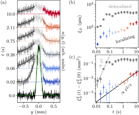
Figure 5: Asymmetric-disorder measurement for variable expansion time and fixed $\langle V\rangle=$691\text{\,}\mathrm{n}\mathrm{K}$\times k_{\mathrm{B}}$. (a) Density profiles $n$ for increasing expansion time $t$ (bottom to top, left axis). The colored lines at the right side (dark-gray lines at the left side) denote the part in $+y$ ($-y$) direction outside the extent of the cloud at $t=0$, which itself is plotted as light-gray lines around $y=0$. The outer regions are fitted with exponential functions (left: black dashed lines, right: black dotted lines) The bottom-most line plot (black line) shows the $t=0$ density profile and a Gaussian fit (green dashed line). The density scale (right axis) is the same for all profiles. (b) Cloud-extension length scale $\xi_{\pm}$ as extracted from density-profile fits over time. Gray squares show values for $-y$ direction, away from the disorder, and colored circles for $+y$ direction, toward it. Error bars are standard errors from fit. (c) Variance $\xi^{2}_{\pm}(t)-\xi^{2}_{\pm}(0)$ over time with same point colors and symbols as in panel (b). The dashed gray line is a power-law fit with fixed exponent $\alpha=2$ to the first four points of $-y$ direction. The black line is a power-law fit with fixed exponent $\alpha=2/3$ to all plotted $+y$-direction data.

Beyond the cloud width, an additional quantity often used to characterize localization is the localization length $\xi$, i.e., the length scale on which a localized wave function decays. For the non-equilibrium diffusion considered here, the signatures of localization on the atomic density distribution are mixed with signatures from diffusion. In order to unravel the contributions of disorder-induced localization and diffusion, we modify the setup by displacing the speckle-disorder beam toward the $+y$ direction. In this setting, the Fermi gas is initially trapped at the edge of the disorder envelope, and the atom cloud released experiences a strong disorder in the $+y$-direction, and a weak or even negligible disorder in $-y$ direction. The resulting time-resolved density distributions for the maximally achievable disorder strength of $\langle V\rangle\approx$691\text{\,}\mathrm{n}\mathrm{K}$\times k_{\mathrm{B}}$ is shown in Fig. 5. While the resulting density distribution in $-y$-direction can be assumed to be free of any localization effects, the part in $+y$-direction will be affected by localization and diffusion. This version of the setup is reminiscent of transfer-matrix approaches to probe localization, in the sense that the transport of particles moving toward the disorder is limited by the probability of transmission versus reflection.

During a few tens of milliseconds, the cloud shape changes from the trapped-gas profile to a distribution that is compatible to exponential functions on both tails outside of its extension at $t=0$ (see first three line plots from bottom to top in Fig. 5(a)). The low signal-to-noise ratio does not allow us to distinguish between exponential, stretched exponential and power-law functions (see Appendix D). Still, to investigate the behavior of the length scale, we fit an exponential function (see dotted or dashed lines) which yields a cloud-extension length scale $\xi_{\pm}$ along the $\pm y$ direction.

After roughly $60\text{\,}\mathrm{ms}$, $\xi_{-}$ (gray squares) saturates to an equilibrium value, while the other side continues to increase, albeit slowly, see Fig. 5(b)). In fact, the variance $\xi^{2}_{-}(t)-\xi^{2}_{-}(0)$ reveals a ballistic expansion in the direction away from the disorder (gray squares) before saturating. On the other side, the cloud moving toward the disorder expands subdiffusively with exponent $\alpha=2/3$. We confirm this by fitting power laws onto the variances where the only free parameter is the diffusion coefficient, see lines Fig. 5(c)).

The velocity from the ballistic diffusion coefficient is roughly $\sqrt{D_{2}}=\langle v_{-}\rangle\approx$6\text{\,}\mathrm{mm}\text{\,}{\mathrm{s}}^{-1}$$ which is somewhat lower than the velocity found in the disorder-free expansion, see Sec. III.5. This confirms that some amount of disorder is still present in that region, explaining the significantly prolonged observation duration achieved compared to the data set shown in Fig. 4. For the subdiffusion in the strong-disorder region, we find $mD_{2/3}/\hbar=$0.26\pm 0.03\text{\,}\mathrm{s}$^{1/3}$. Since the exponent of $\alpha=2/3$ [38] agrees very well with the data and the fitted diffusion coefficient lies below the quantum of diffusion [42, 22, 23, 39, 38, 43, 44, 45], we conclude that the system must be close to or at the mobility edge as these observations are clear signatures for the Anderson transition.

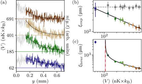
Figure 6: Asymmetric-disorder measurement for variable disorder strength and fixed $t=$1\text{\,}\mathrm{s}$$. (a) Density profiles $n$ for increasing disorder strength $\langle V\rangle$ (bottom to top, left axis). The colored line denotes the part outside the extent of the cloud at $t=0$ (gray lines) and also marks the data fitted by an exponential function (black dotted lines). (b) Cloud-extension length scale $\xi_{-}$ (gray squares) and $\xi_{+}$ (colored circles) direction as extracted from density-profile fits. The black line is a power-law fit of $\xi_{+}$ with exponent $-0.48\,\pm\,0.01$. The gray dashed horizontal line shows $\langle\xi_{-}\rangle$. Error bars are standard errors from fit. (c) Heuristic length scale for localization $\xi_{\mathrm{heur}}$. The black line is a power-law fit of type $|\langle V\rangle-V_{\mathrm{c}}|^{-\nu}$ which yields $\nu=0.50\,\pm\,0.09$ and $V_{\mathrm{c}}=$118\pm 4\text{\,}\mathrm{n}\mathrm{K}$\times k_{\mathrm{B}}$ (red dash-dotted line). Error bars are calculated from error propagation.

The $+y$ extensions of the density profiles after a fixed expansion time of $t=$1\text{\,}\mathrm{s}$$ for increasing disorder strengths are shown in Fig. 6. This duration was chosen as a compromise between ensuring a sufficiently long expansion and hence clear signatures on the one hand, and avoiding losses from collisions with background particles on the other hand. The cloud-extension length scale $\xi_{+}$ appears to follow a power-law behavior (black line in Fig. 6(b)) with an exponent of $-0.48\,\pm\,0.01$. In this direct plot of the length scale $\xi_{+}$, no critical behavior as expected from Anderson theory can be observed. We emphasize, however, that also here the effect of extended states influences the observation in strong disorder. In order to compensate for the contribution of extended states, we introduce a heuristic localization length

$$\xi_{\mathrm{heur}}=\frac{\xi_{+}}{1-\xi_{+}/\langle\xi_{-}\rangle}.$$ (13)

We motivate this length scale as a rescaling of $\xi_{+}$, which we expect to exhibit signatures of localized states, with the diffusion-dominated length scale $\xi_{-}$, which we know to be delocalized. For the latter, we use the average value $\langle\xi_{-}\rangle=$435\pm 31\text{\,}\mathrm{\SIUnitSymbolMicro m}$$ since $\xi_{-}$ does not depend on the disorder strength $\langle V\rangle$. In the limiting case $\xi_{+}\ll\xi_{-}$, the length scale $\xi_{\mathrm{heur}}$ is equal to $\xi_{+}$, indicating that $\xi_{+}$ is close to the localization length, while $\xi_{\mathrm{heur}}\rightarrow\infty$ for $\xi_{+}=\xi_{-}$, and the system behaves as in the disorder-free case.

In Fig. 6(c), $\xi_{\mathrm{heur}}$ is shown with a power-law fit of type $A|\langle V\rangle-V_{\mathrm{c}}|^{-\nu}$, containing a critical disorder strength $V_{\mathrm{c}}$, the critical exponent $\nu$ and a prefactor $A$ as free parameters. This function agrees reasonably well with the coarse of $\xi_{\mathrm{heur}}$ and yields an exponent $\nu=0.50\,\pm\,0.09$ and $V_{\mathrm{c}}=$118\pm 4\text{\,}\mathrm{n}\mathrm{K}$\times k_{\mathrm{B}}$. A critical exponent of $0.5$ has been reported in the literature [83, 84], however, the generally accepted critical exponent for the Anderson transition is $\nu\approx$1.58\text{\,}$$ [38, 5, 4]. The exponent we find does not agree with this value. However, as $\xi_{\mathrm{heur}}$ is a purely heuristic length scale, it is unclear if it is at all expected to exhibit the Anderson critical power law. As mentioned above, we suspect that our system might be on a 1D-3D crossover. Correspondingly, neither pure-1D nor pure-3D Anderson theory could be fitting expectations. Theoretical works that investigate strongly anisotropic settings suggest that reducing the dimensionality enhances localization effects [85, 86] but, to our knowledge, it is so far unexplored how such a crossover influences the critical exponent. We emphasize that this analysis is not supposed to determine the critical exponent but, contrarily, suggests that focusing exclusively on exponential density profiles is not sufficient when investigating Anderson localization.

V Conclusion and Outlook

In summary, we experimentally investigated the competition of diffusion and localization in an ultracold non-interacting Fermi gas with relatively broad initial energy and momentum distributions. We presented and compared four observables for MSD of in-situ images of the ultracold atom cloud which can be used to investigate diffusion and localization. We further carefully examined how our system crosses over from being compatible with pure normal diffusion to a subdiffusion, being influenced by Anderson localization. In a displaced-disorder configuration, we could observe the power law of $t^{2/3}$ that is expected near the mobility edge before the system becomes fully localized [38]. We further emphasize that the observation of density distributions which can be described by exponential functions is not sufficient to identify Anderson localization unequivocally as exponential tails would even be expected in a purely diffusive setting [37, 38].

A thorough investigation of the dimensionality of our setup will be of direct interest as we could map out the supposed 1D-3D crossover by changing the radial trapping frequencies. As our system is generally capable of creating a strongly interacting gas of both bosonic and fermionic nature [87, 88], we could investigate the influence of quantum statistics and thus initial energy distribution, inter-particle interactions, and even superfluidity. In recent years, machine learning (ML) concepts for data analysis in physical systems have shown a widespread use and better performances in detecting anomalous diffusion than other common techniques [46]. Combining this with possible ML regression models, one may extract the physical features of the noisy density profiles in interrelation with the newly presented density histograms. Furthermore, statistical methods for deconvolutions are mostly not robust for discrete PDFs. Here too, ML logistical regression promises extraction of relevant observables [89]. Sampling techniques and data augmentation can be equivalently useful for image and signal processing, in particular when augmentation coincides with the effects expected in the underlying physical system [90].

Appendix A Details on experimental methods

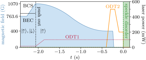
Figure 7: Sketch of the preparation of the spin-polarized gas. The magnetic field (large blue area) pertains to the left axis and the laser powers (ODT1&2, speckle disorder) to the right axis. The black horizontal line shows the Feshbach resonance for the spin mixture in states $\ket{\uparrow},\ket{\downarrow}$ at $B=$832.2\text{\,}\mathrm{G}$$. The time of the push-out beam is shown as a black dash-dotted line.

As stated in the conclusion, our system is able to create strongly interacting gases. More specifically, we usually work with an equal mixture of the two spin states $\ket{\uparrow}\coloneqq\ket{m_{J}=-1/2,m_{I}=1}$ and $\ket{\downarrow}\coloneqq\ket{m_{J}=-1/2,m_{I}=0}$ at high magnetic fields, with $m_{J}$ ($m_{I}$) being the magnetic quantum number of the electronic (nuclear) spin [55]. We can apply magnetic fields of up to $B=$1070\text{\,}\mathrm{G}$$, granting us access to the broad Feshbach resonance around $B=$832.2\text{\,}\mathrm{G}$$ and, therefore, the crossover between Bose-Einstein-condensate (BEC) and Bardeen-Cooper-Schrieffer-type (BCS) superfluidity [91, 92]. Fore more details about our setup, see Refs. [87, 55].

In Fig. 7, a sketch of the preparation of the spin-polarized gas is shown. We start the sequence used for this work by creating a BEC at $B=$763.6\text{\,}\mathrm{G}$$, followed by a slow ramp of $200\text{\,}\mathrm{ms}$ to $B=$1070\text{\,}\mathrm{G}$$. There, deep in the BCS regime where the fermionic pairs are weakly bound and spatially far apart, we apply a push-out laser pulse resonant to state $\ket{\downarrow}$ with a duration of $2\text{\,}\mathrm{\SIUnitSymbolMicro s}$. During that pulse, only roughly $10\text{\,}\%$ of atoms in state $\ket{\uparrow}$ are lost due to resonant scattering, and no measurable amount of $\ket{\downarrow}$ atoms remain.

Afterwards, we deepen the trap by increasing the laser power of ODT1 from the initial $15\text{\,}\mathrm{mW}$ to $100\text{\,}\mathrm{mW}$ and perform a very slow ($1.65\text{\,}\mathrm{s}$) double-parabolic field ramp down to an intermediate field of $B=$400\text{\,}\mathrm{G}$$. This is necessary because the position of our magnetic field center changes significantly with $B$, making this a transport over a distance of more than $300\text{\,}\mathrm{\SIUnitSymbolMicro m}$. Since our non-interacting sample cannot thermalize, any excitations will remain in the gas, which is why this ramp was chosen with such a long timescale. For every step of the sequence until $t=0$, we made sure that no oscillations or unaccounted broadening occur. Further, we never observe atom losses, the only exception being during the push-out pulse.

At that stage, we load our gas into the crossed trap by slowly introducing ODT2 over $100\text{\,}\mathrm{ms}$ until a power of $500\text{\,}\mathrm{mW}$ is reached. Then, we switch off the magnetic field rather quickly during $30\text{\,}\mathrm{ms}$, also in a double-parabolic ramp. We found that switching off the field rapidly rather than slowly induced no measurable excitations. We explain that with the magnetic trap being relatively shallow at that stage ($\omega_{y}<15\times 2\pi\,$Hz), while ODT2’s influence was large during the field shut off (resulting in $\omega_{y}>60\times 2\pi\,$Hz and several hundred $2\pi\,$Hz for the remaining axes).

Once the magnetic field is switched off, the signal-to-noise ratio is significantly reduced due to optical pumping into dark states as described in Refs. [80, 93]. Further, our imaging is aligned and calibrated for high magnetic fields, both of which explain the large noise present in the images.

To determine the atom number accurately, we ran an additional sequence in which we took absorption images after every step as well as after reverting the previous step. By reverting, we ensured that no atoms were actually lost even if the measured atom number was significantly different at $B=$0\text{\,}\mathrm{G}$$ as compared to finite fields. From that measurement, we found an imaging-correction factor of roughly $3.4$, which translated the perceived atom number at zero field to the value we would measure at the field of $B=$763.6\text{\,}\mathrm{G}$$ for which our imaging is calibrated.

Once the field has been switched off, we ramp the laser power of ODT2 down to $200\text{\,}\mathrm{mW}$ during $100\text{\,}\mathrm{ms}$. This finishes the preparation, after which we initialize the expansion at $t=0$ by switching off ODT2 while switching on the disorder. Using acousto-optical modulators, this step happens during less than one microsecond, faster than the timescale of the atom’s motion. Finally, by instead imaging the cloud in situ, we can extract its temperature as described in Refs. [94, 80].

Appendix B Statistical investigation of density distributions

For the theoretical investigation of the qualitative profiles of $p(n,t)$ in the main text, we evaluate the normalized histograms for the continuum

$$\wp(n,t)=\frac{1}{N(t)}\int_{-\infty}^{\infty}\mathrm{d}y\,\delta(n-n(y,y_{0},t)),$$ (14)

where $\int_{w(t)}n\wp(n,t)\,\mathrm{d}n=1$ which is given by the condition $\int_{-\infty}^{\infty}n(y,y_{0},t)=N(t)$. For the remainder of this section, we will fix the peak position to $y_{0}=0$. Furthermore, $\wp(n,t)$ can be thought as a kernel of a probability density function, as $\wp(n,t)$ is expected to show divergences in the continuum leading to $\int_{w(t)}\wp(n,t)\,\mathrm{d}n$ being not convergent. As a kernel, it has all properties of a PDF, besides normalization. Still, evaluating Eq. (14) allows for an easier analytical insight, which will become relevant when we test the control distribution, see Eq. (3). Given an initial unimodal distribution in space without noise, see Eq. (3), the normalized histogram has the form

$$\wp_{\mathrm{Gauss}}(n,t)=\frac{\sqrt{2}\sigma}{n\sqrt{-\mathrm{ln}(\frac{n\sqrt{2\pi\sigma^{2}(t)}}{N(t)})}},$$ (15)

for the support $0<n<\frac{N(t)}{\sqrt{2\pi\sigma^{2}(t)}}$. The two divergencies correspond to the most common occurrences of densities, which are 0 and the peak density. In the noise-free case, the peak density is then trivially given by $n(0,t)=\frac{N(t)}{\sqrt{2\pi\sigma^{2}(t)}}$ for the density centered around zero.

To further estimate the range of unimodal distributions in space, giving divergent flanks in their corresponding histogram, we assume a generalized Gaussian distribution centered around zero

$$n_{\mathrm{gG}}(y,t)=\frac{\nu_{\mathrm{gG}}}{2\sqrt{2\sigma^{2}(t)}\,\Gamma(1/\nu_{\mathrm{gG}})}\mathrm{e}^{-\left(\frac{|y|}{\sqrt{2\sigma^{2}(t)}}\right)^{\nu_{\mathrm{gG}}}},$$ (16)

where $\Gamma(\cdot)$ is the gamma function and $\nu_{\mathrm{gG}}$ is an additional parameter controlling the shape of peak and tails. For $\nu_{\mathrm{gG}}=2$, we restore the normal distribution and, for $\nu_{\mathrm{gG}}=1$, we get a symmetric exponential distribution, as expected in the perfectly localized case [68]. Evaluating the histogram of Eq. (16), we get

$$\wp_{\mathrm{gG}}(n,t,\nu_{\mathrm{gG}})=\frac{2\sqrt{2\sigma^{2}(t)}}{n\nu_{\mathrm{gG}}\left[-\ln{\frac{n\sqrt{2\sigma^{2}(t)}\Gamma(1/\nu_{\mathrm{gG}})}{N(t)\nu_{\mathrm{gG}}}}\right]^{1-1/\nu_{\mathrm{gG}}}},$$ (17)

for the support $0<n<\frac{N(t)\nu_{\mathrm{gG}}}{\sqrt{2\sigma^{2}(t)}\Gamma(1/\nu_{\mathrm{gG}})}$ which restores the $\wp_{\mathrm{Gauss}}$ for $\nu_{\mathrm{gG}}=2$. This distribution has divergent flanks for all $\nu_{\mathrm{gG}}>1$. The divergent flanks in the histogram are necessary for the evaluation of IPW with noise, since the convolution with the noise shows a bimodal profile from which we can approximate the noise-free width and therefore peak density, see Sec. III.4.

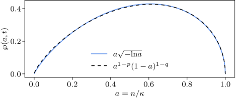
Figure 8: Comparison of inverse kernels of $\wp_{\mathrm{Gauss}}$ (blue solid line) and $\mathrm{Beta}$ (black dashed line), Eq. (18), over $a=n/\kappa$. For $p=0.22$ and $q=0.505$, as used here, the Beta distribution approximates $\wp_{\mathrm{Gauss}}$.

Instead of assuming Gaussian density distributions in space, we may as well model the histogram. In statistics, it is common to model probabilities or random variables in a finite range $(0,n_{\mathrm{max}})$ via a Beta distribution [95]

$$\mathrm{Beta}(p,q,a)=\frac{a^{p-1}\left(1-a\right)^{q-1}}{B(p,q)},$$ (18)

$$\mathrm{for}\ 0<a<1\quad\mathrm{and}\quad B(p,q)=\frac{\Gamma(p)\Gamma(q)}{\Gamma(p+q)}.$$ (19)

where $p$ and $q$ are parameters and depend on the provided density profile. To fit the profile, we will look at the stretched Beta distribution $\kappa\mathrm{Beta}(p,q,\kappa a)$, where $\kappa=n(0,t)=w(t)$ is the stretching factor corresponding to the width $w(t)$ and $n=\kappa a$. If the density profile $n(y,t)$ is unknown, we can either fit or use the method of moments to evaluate $p$ and $q$. If $n(y,t)$ is known, we can fix $p$ and $q$, as shown in Fig. 8 for the exemplary case of a Gaussian, Eq. (15). We may also evaluate the variance of a variable $A\sim\mathrm{Beta}$ following the Beta distribution

$$\mathrm{Var(A)}=\frac{pq}{(p+q)^{2}(p+q+1)}.$$ (20)

Evaluating the variance for the stretched Beta distribution, where $p$, $q$ are assumed constant, we receive $\kappa^{2}\mathrm{Var(A)}$. This means that the change of the variance is completely determined by the stretching factor, which is equal to the width $w(t)$.

Appendix C Numerical investigation of observable performance

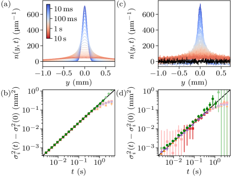
Figure 9: Observable performance on numerically generated data for the (a, b) noise-free and (c, d) noisy case. (a, c) Generated Gaussian line densities over $y$ for different expansion times $t$, see colorbar in (a). (b, d) Extracted $\sigma^{2}_{i}(t)-\sigma^{2}_{i}(0)$ over time $t$. The observables $i$ stand for the Gauss-fit variance “fit” (orange triangles), density-profile variance “Var” (red squares), width from the participation ratio PR (purple hexagons), and IPW (green circles), with same point colors and symbols as in Fig. 3. The black line shows the true $\sigma^{2}$ as simulated for the plotted Gaussians. For the data shown here, $\alpha=1$ and $D_{1}=10\hbar/m$ is used. Errors are computed as for the experimental data. See Sec. III.5 and Fig. 3 for details about the observables.

To further analyze the observable performances, we evaluated numerically generated density profiles. We begin by generating a Gaussian density, see Eq. (3), over $y$ from a Gauss fit to the trapped-gas profile from the experimental data. We use a $y$ axis analogous to the axis in the experiment to simulate the resolution and image size of our imaging system. For a given list of expansion times $t$, we generate new Gaussians for every $t$ while changing their $\sigma(t)$ according to Eq. (2), simulating a diffusive expansion. Depending on the case, we use $\alpha=1$ or $2$ and any arbitrary $D_{\alpha}$. Before we evaluate the line densities in the same way as for the experimental data, we can optionally add random white (Gaussian) noise, which we usually set to have the same $\sigma_{\mathrm{noise}}$ as the camera noise, see Fig. 2 and Sec. III.4. As in the experiment, we generate 50 images per setting that are averaged and then evaluated further. In Fig. 9, the noise-free density distributions are shown in (a) and the data with noise in (b). The various $\sigma^{2}_{i}$ for the respective cases are plotted in (c) and (d).

Compared to the experimental data, this investigation has several advantages. First, we can switch off the “camera” noise to investigate its influence on the results directly. Similarly, it is significantly faster to generate more data numerically compared to running the experiment, yielding a better statistics. Second, we can increase or decrease both resolution and “image” size, which allows us to get rid of or enhance finite-size effects. Further, since we define how the drawn densities expand in time, we have a true reference to compare the inferred results to (see solid line in Fig. 9(c, d)). Also, we are not limited by long-time atom losses.

Note that this investigation effectively only yields information about how well a perfect (albeit noisy) Gaussian can be evaluated during an expansion similar to that of our experiment. As we interpret our cloud as being partially localized and therefore potentially bimodal, this is not captured by this effort. It would be, however, interesting how different cloud shapes (see e.g. the profiles shown in Fig. 10) would be evaluated. Nevertheless, we can infer useful qualitative information about the observable performance, i.e. that $\sigma^{2}_{\mathrm{Var}}$ appears to be very susceptible to noise in general. Further, independent of noise but enhanced by it, all observables have the tendency to curve below the simulated $\sigma^{2}$, except for IPW which is observed to do the opposite. Nevertheless, with sensible fit-range choices, all observables perform perfectly in determining both diffusion quantities if no noise is present. For the results in the case with noise, see Fig. 3(c). Overall, we find that the combination of such a supporting numerical investigation with the evaluation of the experimental data yields a good overview of the observable performances.

Appendix D Density profiles

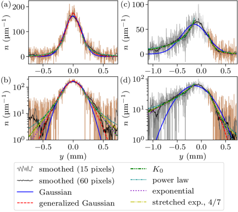
Figure 10: Analysis of density profiles for expansion in symmetric (a, b) and asymmetric (c, d) disorder. Several expectations for density profiles have been fitted to the respective data, see legend on bottom. Additionally, smoothed data computed by convolution with a box function of given width is shown for enhanced visibility. Note that both (a, b) and (c, d) display roughly 800 camera pixels along $y$. (a) Data from $\langle V\rangle\approx$642\text{\,}\mathrm{n}\mathrm{K}$\times k_{\mathrm{B}}$ and $t\approx$0.82\text{\,}\mathrm{s}$$. For both the zeroth-order Hankel function $K_{0}$ [38, 37] and the exponential function, the region $|y|<$0.15\text{\,}\mathrm{mm}$$ was excluded. The exponential function was fitted independently for both directions $\pm y$. (b) Same as (a) but with logarithmic density scale. (c) Data from $\langle V\rangle\approx$691\text{\,}\mathrm{n}\mathrm{K}$\times k_{\mathrm{B}}$ and $t=$1\text{\,}\mathrm{s}$$. All shown functions were fitted independently for both directions $\pm y$. Segmentation along $y$ is identical to Figs. 5 and  6. (d) Same as (c) but with logarithmic density scale.

In this section, we compare several expectations of density profiles fitted to the recorded line densities $n(y)$. For that, we use two representative examples. The first, shown in Fig. 10(a, b), is from the expansion in strong symmetrical disorder, see Sec. IV.1. The second, shown in Fig. 10(c, d), is from the expansion in strong asymmetrical disorder, see Sec. IV.1. Both images were taken for an expansion time of $t\approx$1\text{\,}\mathrm{s}$$ and have been averaged from 50 realizations, see Sec. II for more details. We plot each image in both linear and logarithmic density scales to emphasize the exponential character of the different density profiles, or the lack thereof. Additionally, we show our data after smoothing it via a convolution with a top-hat kernel, see gray lines. For the width of the smoothing kernel, we use both 15 and 60 pixels. Note that we only show the smoothed line plots but do not evaluate it, all shown fits are performed to the recorded densities. In the following, we discuss the choice of density profiles.

To begin with, we fit a Gaussian function, see Eq. (3), as it is the basis for all observables described in Sec. III and is generally a good albeit naive approximation for our density profile. For a Bose-Einstein condensate (BEC) undergoing diffusion, Refs. [37, 38] derive a zeroth-order modified Hankel function $K_{0}$ and, as Ref. [38] states, expansion of a degenerate Fermi gas is not expected to look very different. Therefore, we fit $K_{0}$ to the distribution tails. Note that this function is approximated well by an exponential function for large distance to the origin, meaning a purely diffusive, delocalized BEC is already expected to exhibit exponential tails. Further, as it is the general expectation for an Anderson-localized density profile, we fit an exponential function. Contrarily, Ref. [39] claims a stretched-exponential function as the density profile for the case of diffusive spread with an energy-dependent diffusion coefficient. Note that, for the fits presented here, we use the same exponent of 4/7. The authors further add that the tails should follow a power law in the localization scenario. Finally, we fit a generalized Gaussian, see Eq. (16). This function includes an additional exponent $\nu_{\mathrm{gG}}$ in the argument compared to the Gaussian and can be used to indicate the transition between a normal and exponential distribution [16].

As can be seen in Fig. 10, all density distributions are, in principle, compatible to the experimental data due to the large noise. For the symmetric disorder, see Sec. IV.1, the generalized Gaussian appears (exponent of $\nu_{\mathrm{gG}}\approx 1.50$) closest to the data, which is expected as it has the largest amount of free parameters. The Gaussian function underestimates the tails very slightly while most of the other functions describe it relatively well. For completeness’ sake, the power-law fit yields an exponent of $\nu_{\mathrm{pl}}\approx-2.63$ ($\nu_{\mathrm{pl}}\approx-2.85$) for the tail toward the $+y$ ($-y$) direction.

For the asymmetric disorder which is displaced toward the $+y$ direction, see Sec. IV.2, the Gaussian function exhibits the largest discrepancy. However, all other functions describe the outer regions (dark gray and brown lines outside $y=0$) very well. Here, the generalized Gaussian yields an exponent of $\nu_{\mathrm{gG}}\approx 1.29$ ($\nu_{\mathrm{gG}}\approx 0.76$) for the $+y$ ($-y$) direction, while the power-law exponent is found to fit best at $\nu_{\mathrm{pl}}\approx-2.71$ ($\nu_{\mathrm{pl}}\approx-1.20$).

We conclude that the low signal-to-noise ratio does not allow for a reliable analysis of the distribution shape in general, but especially the tails. In fact, this was the motivation for the careful investigation of subdiffusion.

Appendix E Localized fraction

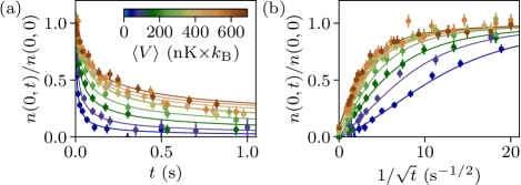
Figure 11: Determining the localized fraction $f_{\mathrm{loc}}$. (a) Relative peak density $n(t)/n(0)$ (circles) over expansion time $t$. Lines are fits with the anomalous-diffusion model Eq. (22) where $f_{\mathrm{loc}}$, the value for $t\rightarrow\infty$ is the only free parameter. Errors are calculated from error propagation. (b) Plotting $n(t)/n(0)$ over the inverse square root of time visualizes $f_{\mathrm{loc}}$ as the density-axis intercept (crosses).

As introduced in Ref. [22], the localized fraction estimates the amount of atoms at the cloud peak that would not have diffused away due to being localized,

$$f_{\mathrm{loc}}=\lim_{t\to\infty}\frac{n(0,t)}{n(0,0)}.$$ (21)

We modify its computation to fit our expansion along a single dimension and implemented the full anomalous-diffusion power law as in Eq. (2) by using the model

$$\frac{n(0,t)}{n(0,0)}=f_{\mathrm{loc}}+(1-f_{\mathrm{loc}})\sqrt{\frac{\sigma^{2}(0)}{2D_{\alpha}t^{\alpha}+\sigma^{2}(0)}},$$ (22)

where we fix the diffusion exponent $\alpha$ and coefficient $D_{\alpha}$ to the values we extract as described in Sec. III and use $\sigma(0)=$53\text{\,}\mathrm{\SIUnitSymbolMicro m}$$ (see Sec. III.5). For the relative peak density $n(0,t)/n(0,0)$, we use the approximation of $n(t)\approx w(t)-w_{\mathrm{noise}}$ mentioned in Sec. III.4, multiplied by the factor $N(0)/N(t)$ to compensate for atom losses. With that, $f_{\mathrm{loc}}$ is extracted as the only free parameter from fitting the right side of Eq. (22), see lines in Fig. 11.

References

- Anderson [1958] P. W. Anderson, Absence of Diffusion in Certain Random Lattices, Physical Review 109, 1492 (1958).
- Abrahams [2010] E. Abrahams, ed., 50 Years of Anderson Localization (World Scientific, Singapore, 2010).
- MacKinnon and Kramer [1983] A. MacKinnon and B. Kramer, The scaling theory of electrons in disordered solids: Additional numerical results, Zeitschrift für Physik B Condensed Matter 53, 1 (1983).
- Slevin and Ohtsuki [1999] K. Slevin and T. Ohtsuki, Corrections to Scaling at the Anderson Transition, Physical Review Letters 82, 382 (1999).
- Lopez et al. [2012] M. Lopez, J.-F. Clément, P. Szriftgiser, J. C. Garreau, and D. Delande, Experimental Test of Universality of the Anderson Transition, Physical Review Letters 108, 095701 (2012).
- Wiersma et al. [1997] D. S. Wiersma, P. Bartolini, A. Lagendijk, and R. Righini, Localization of light in a disordered medium, Nature 390, 671 (1997).
- Scheffold et al. [1999] F. Scheffold, R. Lenke, R. Tweer, and G. Maret, Localization or classical diffusion of light?, Nature 398, 206 (1999).
- Störzer et al. [2006] M. Störzer, P. Gross, C. M. Aegerter, and G. Maret, Observation of the critical regime near anderson localization of light, Phys. Rev. Lett. 96, 063904 (2006).
- Schwartz et al. [2007] T. Schwartz, G. Bartal, S. Fishman, and M. Segev, Transport and Anderson localization in disordered two-dimensional photonic lattices, Nature 446, 52 (2007).
- Mafi and Ballato [2021] A. Mafi and J. Ballato, Review of a Decade of Research on Disordered Anderson Localizing Optical Fibers, Frontiers in Physics 9 (2021).
- Weaver [1990] R. Weaver, Anderson localization of ultrasound, Wave Motion 12, 129 (1990).
- Hu et al. [2008] H. Hu, A. Strybulevych, J. H. Page, S. E. Skipetrov, and B. A. van Tiggelen, Localization of ultrasound in a three-dimensional elastic network, Nature Physics 4, 945 (2008).
- Goïcoechea et al. [2020] A. Goïcoechea, S. E. Skipetrov, and J. H. Page, Suppression of transport anisotropy at the Anderson localization transition in three-dimensional anisotropic media, Physical Review B 102, 220201 (2020).
- Dalichaouch et al. [1991] R. Dalichaouch, J. P. Armstrong, S. Schultz, P. M. Platzman, and S. L. McCall, Microwave localization by two-dimensional random scattering, Nature 354, 53 (1991).
- Chabanov et al. [2000] A. A. Chabanov, M. Stoytchev, and A. Z. Genack, Statistical signatures of photon localization, Nature 404, 850 (2000).
- Roati et al. [2008] G. Roati, C. D’Errico, L. Fallani, M. Fattori, C. Fort, M. Zaccanti, G. Modugno, M. Modugno, and M. Inguscio, Anderson localization of a non-interacting Bose–Einstein condensate, Nature 453, 895 (2008).
- Billy et al. [2008] J. Billy, V. Josse, Z. Zuo, A. Bernard, B. Hambrecht, P. Lugan, D. Clément, L. Sanchez-Palencia, P. Bouyer, and A. Aspect, Direct observation of Anderson localization of matter waves in a controlled disorder, Nature 453, 891 (2008).
- White et al. [2020] D. H. White, T. A. Haase, D. J. Brown, M. D. Hoogerland, M. S. Najafabadi, J. L. Helm, C. Gies, D. Schumayer, and D. A. W. Hutchinson, Observation of two-dimensional Anderson localisation of ultracold atoms, Nature Communications 11, 4942 (2020).
- Shamailov [2021] S. S. Shamailov, Comment on ”Observation of two-dimensional Anderson localisation of ultracold atoms” (2021).
- Najafabadi et al. [2021] M. S. Najafabadi, D. Schumayer, and D. A. W. Hutchinson, Effects of disorder upon transport and Anderson localization in a finite, two-dimensional Bose gas, Physical Review A 104, 063311 (2021).
- Kondov et al. [2011] S. S. Kondov, W. R. McGehee, J. J. Zirbel, and B. DeMarco, Three-Dimensional Anderson Localization of Ultracold Matter, Science 334, 66 (2011).
- Jendrzejewski et al. [2012] F. Jendrzejewski, A. Bernard, K. Müller, P. Cheinet, V. Josse, M. Piraud, L. Pezzé, L. Sanchez-Palencia, A. Aspect, and P. Bouyer, Three-dimensional localization of ultracold atoms in an optical disordered potential, Nature Physics 8, 398 (2012).
- Semeghini et al. [2015] G. Semeghini, M. Landini, P. Castilho, S. Roy, G. Spagnolli, A. Trenkwalder, M. Fattori, M. Inguscio, and G. Modugno, Measurement of the mobility edge for 3D Anderson localization, Nature Physics 11, 554 (2015).
- Zhao et al. [2020a] Y. Zhao, D. Feng, Y. Hu, S. Guo, and J. Sirker, Entanglement dynamics in the three-dimensional anderson model, Phys. Rev. B 102, 195132 (2020a).
- Sierant et al. [2020] P. Sierant, D. Delande, and J. Zakrzewski, Thouless time analysis of anderson and many-body localization transitions, Phys. Rev. Lett. 124, 186601 (2020).
- Šuntajs et al. [2021] J. Šuntajs, T. Prosen, and L. Vidmar, Spectral properties of three-dimensional anderson model, Annals of Physics 435, 168469 (2021).
- Kiefer-Emmanouilidis et al. [2020a] M. Kiefer-Emmanouilidis, R. Unanyan, M. Fleischhauer, and J. Sirker, Evidence for unbounded growth of the number entropy in many-body localized phases, Phys. Rev. Lett. 124, 243601 (2020a).
- Kiefer-Emmanouilidis et al. [2021a] M. Kiefer-Emmanouilidis, R. Unanyan, M. Fleischhauer, and J. Sirker, Slow delocalization of particles in many-body localized phases, Phys. Rev. B 103, 024203 (2021a).
- Šuntajs et al. [2020a] J. Šuntajs, J. Bonča, T. c. v. Prosen, and L. Vidmar, Quantum chaos challenges many-body localization, Phys. Rev. E 102, 062144 (2020a).
- Šuntajs et al. [2020b] J. Šuntajs, J. Bonča, T. c. v. Prosen, and L. Vidmar, Ergodicity breaking transition in finite disordered spin chains, Phys. Rev. B 102, 064207 (2020b).
- Abanin et al. [2021] D. Abanin, J. Bardarson, G. De Tomasi, S. Gopalakrishnan, V. Khemani, S. Parameswaran, F. Pollmann, A. Potter, M. Serbyn, and R. Vasseur, Distinguishing localization from chaos: Challenges in finite-size systems, Annals of Physics 427, 168415 (2021).
- Ghosh and Žnidarič [2022] R. Ghosh and M. Žnidarič, Resonance-induced growth of number entropy in strongly disordered systems, Phys. Rev. B 105, 144203 (2022).
- Luitz and Lev [2020] D. J. Luitz and Y. B. Lev, Absence of slow particle transport in the many-body localized phase, Phys. Rev. B 102, 100202 (2020).
- Léonard et al. [2023] J. Léonard, S. Kim, M. Rispoli, A. Lukin, R. Schittko, J. Kwan, E. Demler, D. Sels, and M. Greiner, Probing the onset of quantum avalanches in a many-body localized system, Nature Physics 19, 481 (2023).
- Sels and Polkovnikov [2021] D. Sels and A. Polkovnikov, Dynamical obstruction to localization in a disordered spin chain, Phys. Rev. E 104, 054105 (2021).
- Sels [2022] D. Sels, Bath-induced delocalization in interacting disordered spin chains, Phys. Rev. B 106, L020202 (2022).
- Shapiro [2007] B. Shapiro, Expansion of a Bose-Einstein Condensate in the Presence of Disorder, Physical Review Letters 99, 060602 (2007).
- Shapiro [2012] B. Shapiro, Cold atoms in the presence of disorder, Journal of Physics A: Mathematical and Theoretical 45, 143001 (2012).
- Müller and Shapiro [2014] C. A. Müller and B. Shapiro, Comment on “Three-Dimensional Anderson Localization in Variable Scale Disorder”, Physical Review Letters 113, 099601 (2014).
- Robert-de Saint-Vincent et al. [2010] M. Robert-de Saint-Vincent, J.-P. Brantut, B. Allard, T. Plisson, L. Pezzé, L. Sanchez-Palencia, A. Aspect, T. Bourdel, and P. Bouyer, Anisotropic 2D Diffusive Expansion of Ultracold Atoms in a Disordered Potential, Physical Review Letters 104, 220602 (2010).
- Scholak et al. [2014] T. Scholak, T. Wellens, and A. Buchleitner, Spectral backbone of excitation transport in ultracold Rydberg gases, Physical Review A 90, 063415 (2014).
- Kuhn et al. [2007] R. C. Kuhn, O. Sigwarth, C. Miniatura, D. Delande, and C. A. Müller, Coherent matter wave transport in speckle potentials, New Journal of Physics 9, 161 (2007).
- Patel et al. [2020] P. B. Patel, Z. Yan, B. Mukherjee, R. J. Fletcher, J. Struck, and M. W. Zwierlein, Universal sound diffusion in a strongly interacting Fermi gas, Science 370, 1222 (2020).
- Sommer et al. [2011] A. Sommer, M. Ku, G. Roati, and M. W. Zwierlein, Universal spin transport in a strongly interacting Fermi gas, Nature 472, 201 (2011).
- Enss and Haussmann [2012] T. Enss and R. Haussmann, Quantum Mechanical Limitations to Spin Diffusion in the Unitary Fermi Gas, Physical Review Letters 109, 195303 (2012).
- Muñoz-Gil et al. [2021] G. Muñoz-Gil, G. Volpe, M. A. Garcia-March, E. Aghion, A. Argun, C. B. Hong, T. Bland, S. Bo, J. A. Conejero, N. Firbas, î Garibo i Orts, A. Gentili, Z. Huang, J.-H. Jeon, H. Kabbech, Y. Kim, P. Kowalek, D. Krapf, H. Loch-Olszewska, M. A. Lomholt, J.-B. Masson, P. G. Meyer, S. Park, B. Requena, I. Smal, T. Song, J. Szwabiński, S. Thapa, H. Verdier, G. Volpe, A. Widera, M. Lewenstein, R. Metzler, and C. Manzo, Objective comparison of methods to decode anomalous diffusion, Nature Communications 12, 6253 (2021).
- Metzler et al. [2022] R. Metzler, A. Rajyaguru, and B. Berkowitz, Modelling anomalous diffusion in semi-infinite disordered systems and porous media, New Journal of Physics 24, 123004 (2022).
- Metzler and Klafter [2000] R. Metzler and J. Klafter, The random walk’s guide to anomalous diffusion: a fractional dynamics approach, Physics Reports 339, 1 (2000).
- Mangalam et al. [2023] M. Mangalam, R. Metzler, and D. G. Kelty-Stephen, Ergodic characterization of nonergodic anomalous diffusion processes, Physical Review Research 5, 023144 (2023).
- Levi et al. [2012] L. Levi, Y. Krivolapov, S. Fishman, and M. Segev, Hyper-transport of light and stochastic acceleration by evolving disorder, Nature Physics 8, 912 (2012).
- Beilin et al. [2010] L. Beilin, E. Gurevich, and B. Shapiro, Diffusion of cold-atomic gases in the presence of an optical speckle potential, Physical Review A 81, 033612 (2010).
- Top et al. [2021] F. î Top, Y. Margalit, and W. Ketterle, Spin-polarized fermions with -wave interactions, Physical Review A 104, 043311 (2021).
- Reinaudi et al. [2007] G. Reinaudi, T. Lahaye, Z. Wang, and D. Guéry-Odelin, Strong saturation absorption imaging of dense clouds of ultracold atoms, Optics Letters 32, 3143 (2007).
- Ries et al. [2015] M. G. Ries, A. N. Wenz, G. Zürn, L. Bayha, I. Boettcher, D. Kedar, P. A. Murthy, M. Neidig, T. Lompe, and S. Jochim, Observation of Pair Condensation in the Quasi-2D BEC-BCS Crossover, Physical Review Letters 114, 230401 (2015).
- Nagler et al. [2020] B. Nagler, M. Radonjić, S. Barbosa, J. Koch, A. Pelster, and A. Widera, Cloud shape of a molecular Bose–Einstein condensate in a disordered trap: a case study of the dirty boson problem, New Journal of Physics 22, 033021 (2020).
- Nagler et al. [2022] B. Nagler, S. Barbosa, J. Koch, G. Orso, and A. Widera, Observing the loss and revival of long-range phase coherence through disorder quenches, Proceedings of the National Academy of Sciences 119 (2022).
- Pilati et al. [2010] S. Pilati, S. Giorgini, M. Modugno, and N. Prokof’ev, Dilute Bose gas with correlated disorder: a path integral Monte Carlo study, New Journal of Physics 12, 073003 (2010).
- Sanchez-Palencia et al. [2008] L. Sanchez-Palencia, D. Clément, P. Lugan, P. Bouyer, and A. Aspect, Disorder-induced trapping versus Anderson localization in Bose–Einstein condensates expanding in disordered potentials, New Journal of Physics 10, 045019 (2008).
- Delande and Orso [2014] D. Delande and G. Orso, Mobility Edge for Cold Atoms in Laser Speckle Potentials, Physical Review Letters 113, 060601 (2014).
- Kindermann et al. [2017] F. Kindermann, A. Dechant, M. Hohmann, T. Lausch, D. Mayer, F. Schmidt, E. Lutz, and A. Widera, Nonergodic diffusion of single atoms in a periodic potential, Nature Physics 13, 137 (2017).
- D’Errico et al. [2013] C. D’Errico, M. Moratti, E. Lucioni, L. Tanzi, B. Deissler, M. Inguscio, G. Modugno, M. B. Plenio, and F. Caruso, Quantum diffusion with disorder, noise and interaction, New Journal of Physics 15, 045007 (2013).
- Vilk et al. [2022] O. Vilk, E. Aghion, T. Avgar, C. Beta, O. Nagel, A. Sabri, R. Sarfati, D. K. Schwartz, M. Weiss, D. Krapf, R. Nathan, R. Metzler, and M. Assaf, Unravelling the origins of anomalous diffusion: From molecules to migrating storks, Physical Review Research 4, 033055 (2022).
- Dyson [2004] F. Dyson, A meeting with Enrico Fermi, Nature 427, 297 (2004).
- Mayer et al. [2010] J. Mayer, K. Khairy, and J. Howard, Drawing an elephant with four complex parameters, American Journal of Physics 78, 648 (2010).
- Bell and Dean [1970] R. J. Bell and P. Dean, Atomic vibrations in vitreous silica, Discussions of the Faraday Society 50, 55 (1970).
- Edwards and Thouless [1972] J. T. Edwards and D. J. Thouless, Numerical studies of localization in disordered systems, Journal of Physics C: Solid State Physics 5, 807 (1972).
- Dikopoltsev et al. [2022] A. Dikopoltsev, S. Weidemann, M. Kremer, A. Steinfurth, H. H. Sheinfux, A. Szameit, and M. Segev, Observation of Anderson localization beyond the spectrum of the disorder, Science Advances 8, eabn7769 (2022).
- Laflorencie [2022] N. Laflorencie, Entanglement Entropy and Localization in Disordered Quantum Chains, in Entanglement in Spin Chains: From Theory to Quantum Technology Applications, Quantum Science and Technology, edited by A. Bayat, S. Bose, and H. Johannesson (Springer International Publishing, Cham, 2022) pp. 61–87.
- Kramer and MacKinnon [1993] B. Kramer and A. MacKinnon, Localization: theory and experiment, Reports on Progress in Physics 56, 1469 (1993).
- Hartman et al. [2017] T. Hartman, S. A. Hartnoll, and R. Mahajan, Upper bound on diffusivity, Phys. Rev. Lett. 119, 141601 (2017).
- Lukin et al. [2019] A. Lukin, M. Rispoli, R. Schittko, M. E. Tai, A. M. Kaufman, S. Choi, V. Khemani, J. Léonard, and M. Greiner, Probing entanglement in a many-body–localized system, Science 364, 256 (2019).
- Rispoli et al. [2019] M. Rispoli, A. Lukin, R. Schittko, S. Kim, M. E. Tai, J. Léonard, and M. Greiner, Quantum critical behaviour at the many-body localization transition, Nature 573, 385 (2019).
- Contessi et al. [2023] D. Contessi, A. Recati, and M. Rizzi, Phase diagram detection via gaussian fitting of number probability distribution, Phys. Rev. B 107, L121403 (2023).
- Calabrese et al. [2020] P. Calabrese, M. Collura, G. D. Giulio, and S. Murciano, Full counting statistics in the gapped spin chain, Europhysics Letters 129, 60007 (2020).
- Kiefer-Emmanouilidis et al. [2020b] M. Kiefer-Emmanouilidis, R. Unanyan, J. Sirker, and M. Fleischhauer, Bounds on the entanglement entropy by the number entropy in non-interacting fermionic systems, SciPost Physics 8, 083 (2020b).
- Kiefer-Emmanouilidis et al. [2021b] M. Kiefer-Emmanouilidis, R. Unanyan, M. Fleischhauer, and J. Sirker, Unlimited growth of particle fluctuations in many-body localized phases, Annals of Physics , 168481 (2021b).
- Zhao et al. [2020b] Y. Zhao, D. Feng, Y. Hu, S. Guo, and J. Sirker, Entanglement dynamics in the three-dimensional Anderson model, Physical Review B 102, 195132 (2020b).
- Park et al. [2021] K.-W. Park, J. Kim, J. Seo, S. Moon, and K. Jeong, Indicators of wavefunction (de)localisation for avoided crossing in a quadrupole quantum billiard, Journal of Physics Communications 5, 115009 (2021).
- Mark F Schilling and Watkins [2002] A. E. W. Mark F Schilling and W. Watkins, Is human height bimodal?, The American Statistician 56, 223 (2002), https://doi.org/10.1198/00031300265 .
- Kinast [2006] J. M. Kinast, Thermodynamics and superfluidity of a strongly interacting Fermi gas, Ph.D. thesis, Duke University (2006).
- Wegner [1976] F. J. Wegner, Electrons in disordered systems. Scaling near the mobility edge, Zeitschrift für Physik B Condensed Matter 25, 327 (1976).
- Abrahams et al. [1979] E. Abrahams, P. W. Anderson, D. C. Licciardello, and T. V. Ramakrishnan, Scaling Theory of Localization: Absence of Quantum Diffusion in Two Dimensions, Physical Review Letters 42, 673 (1979).
- Aegerter et al. [2006] C. M. Aegerter, M. Störzer, and G. Maret, Experimental determination of critical exponents in Anderson localisation of light, Europhysics Letters (EPL) 75, 562 (2006).
- Schuster [1978] H. G. Schuster, On a relation between the mobility edge problem and an isotropic model, Zeitschrift für Physik B Condensed Matter 31, 99 (1978).
- Zhang et al. [1990] Z.-Q. Zhang, Q.-J. Chu, W. Xue, and P. Sheng, Anderson localization in anisotropic random media, Physical Review B 42, 4613 (1990).
- Chu and Zhang [1993] Q.-J. Chu and Z.-Q. Zhang, Anderson localization in an anisotropic model, Physical Review B 48, 10761 (1993).
- Gänger et al. [2018] B. Gänger, J. Phieler, B. Nagler, and A. Widera, A versatile apparatus for fermionic lithium quantum gases based on an interference-filter laser system, Review of Scientific Instruments 89, 093105 (2018).
- Koch et al. [2023] J. Koch, K. Menon, E. Cuestas, S. Barbosa, E. Lutz, T. Fogarty, T. Busch, and A. Widera, A quantum engine in the BEC–BCS crossover, Nature 621, 723 (2023).
- Carroll and Hall [1988] R. J. Carroll and P. Hall, Optimal rates of convergence for deconvolving a density, Journal of the American Statistical Association 83, 1184 (1988).
- Palaiodimopoulos et al. [2023] N. E. Palaiodimopoulos, V. F. Rey, M. Tschöpe, C. Jörg, P. Lukowicz, and M. Kiefer-Emmanouilidis, Quantum inspired image augmentation applicable to waveguides and optical image transfer via anderson localization (2023), arXiv:2302.10138 [cond-mat.dis-nn] .
- Grimm [2007] R. Grimm, Ultracold Fermi gases in the BEC-BCS crossover: a review from the Innsbruck perspective, arXiv:cond-mat/0703091 (2007).
- Zürn et al. [2013] G. Zürn, T. Lompe, A. N. Wenz, S. Jochim, P. S. Julienne, and J. M. Hutson, Precise Characterization of 6Li Feshbach Resonances Using Trap-Sideband-Resolved RF Spectroscopy of Weakly Bound Molecules, Physical Review Letters 110, 135301 (2013).
- Gehm [2003] M. E. Gehm, Preparation of an optically-trapped degenerate Fermi gas of 6Li: Finding the route to degeneracy, Ph.D. thesis, Duke University (2003).
- Hadzibabic et al. [2002] Z. Hadzibabic, C. Stan, K. Dieckmann, S. Gupta, M. Zwierlein, A. Görlitz, and W. Ketterle, Two-species mixture of quantum degenerate bose and fermi gases, Physical review letters 88, 160401 (2002).
- Gupta and Nadarajah [2004] A. Gupta and S. Nadarajah, Handbook of Beta Distribution and Its Applications, Statistics: A Series of Textbooks and Monographs (Taylor & Francis, 2004).