Computerized Tomography and Reproducing Kernels

Abstract

The X-ray transform is one of the most fundamental integral operators in image processing and reconstruction. In this article, we revisit its mathematical formalism, and propose an innovative approach making use of Reproducing Kernel Hilbert Spaces (RKHS). Within this framework, the X-ray transform can be considered as a natural analogue of Euclidean projections. The RKHS framework considerably simplifies projection image interpolation, and leads to an analogue of the celebrated representer theorem for the problem of tomographic reconstruction. It leads to methodology that is dimension-free and stands apart from conventional filtered back-projection techniques, as it does not hinge on the Fourier transform. It also allows us to establish sharp stability results at a genuinely functional level, but in the realistic setting where the data are discrete and noisy. The RKHS framework is amenable to any reproducing kernel on a unit ball, affording a high level of generality. When the kernel is chosen to be rotation-invariant, one can obtain explicit spectral representations which elucidate the regularity structure of the associated Hilbert spaces, and one can also solve the reconstruction problem at the same computational cost as filtered back-projection.

1 Introduction

Since its inception in the 1970s, the technique of Computerized Tomography (CT) has evolved considerably, becoming a vital tool in fields ranging from radiology to structure biology, and various scientific disciplines [31, 8]. This method enables the visualization of an object’s internal features through projection images. At the core of this technology lies the X-ray transform $\mathscr{P}_{R}$, a mathematical operation that, at a given orientation $R\in SO(n)$, maps an original object $f:\mathbb{R}^{n}\rightarrow\mathbb{R}$ to a tomograph through a line integral:

$$\mathscr{P}_{R}f(\mathbf{x})=\int_{-\infty}^{+\infty}f(R^{\top}[\mathbf{x}:z])\mathrm{d}z,$$

where $[\mathbf{x}:z]\in\mathbb{R}^{n}$ denotes the concatenation of $\mathbf{x}\in\mathbb{R}^{n-1}$ with $z\in\mathbb{R}^{1}$. The X-ray transform, in essence, calculates the line integral of an object’s density along the axis $\mathbf{r}:=R^{\top}e_{n}$ of orientation. The collection of projection images $\mathscr{P}f$ is often referred to as a sinogram because the X-ray transform of an off-center point source generates a sinusoidal wave pattern, as depicted in Fig. 1. The fundamental task in tomography is to reconstruct an unknown $f$ from a series of projection images $g_{i}=\mathscr{P}_{R_{i}}f+W_{i}$ captured at various orientations $R_{i}\in SO(n),\,1\leq i\leq N$, often with noise contamination. In practical scenarios, each projection image is discretized within a finite number of mesh points $\mathbf{x}_{j}\in\mathbb{R}^{n-1},\,1\leq j\leq M$, rendering the available data as $y_{ij}=g_{i}(\mathbf{x}_{j})=\mathscr{P}_{R_{i}}f(\mathbf{x}_{j})+\varepsilon_{ij}$. To differentiate between these two setups, we will refer to the first one as the continuous setup and the latter as the discrete setup.

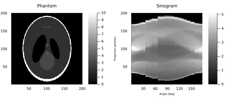
Figure 1: Discretized sinogram at randomly chosen $N=40$ angles over $180^{\circ}$ of the 2D Shepp-Logan phantom.

The X-ray transform coincides with the Radon transform when $n=2$, and a variety of reconstruction methods have been developed within the weighted $\mathcal{L}_{2}$ setting in the continuous setup, see [20] and references therein. In this framework, the standard reconstruction procedure involves two basic steps: interpolating the projection images to generate a sinogram and subsequently backprojecting the sinogram to recover the original image. A reliable sinogram interpolant should satisfy two essential conditions: the compatibility principle and the moment condition, commonly referred to jointly as the Helgason-Ludwig Consistency Conditions (HLCC, see Theorem 2.9). Once the sinogram is successfully generated following the HLCC by restricting resolution [12], the backprojection is performed to reconstruct the image. However, naïve backprojection is not invertible, so the sinogram should be filtered before backprojection – hence the term Filtered Backprojection (FBP)– an approach upon which the majority of reconstruction algorithms rely. In higher dimensions ($n\geq 3$), however, the inversion formula for the sinogram becomes impractical [19], as the X-ray transform has a large null space, while only a finite number of projection images can be observed in practice. One approach to address this ill-posedness is to employ Tikhonov regularization or use a finite number of basis functions obtained from the Singular Value Decomposition (SVD) of the X-ray transform [14], where these functions essentially amount to the multiplication of an orthogonal polynomial in radial direction and a spherical harmonic in angular direction [18].

In the context of inverse problems, it is crucial to understand the stability of reconstruction when dealing with noisy data [9]. In the $\mathcal{L}_{2}$ setting, the inverse operator is unbounded, making reconstructed images vulnerable to small measurement errors. Thus, in order to achieve better estimates of reconstruction stability for the Radon and the X-ray transform, various works [19, 26] have formulated the range space as being the completion of the Schwarz space with respect to a specific norm [25]. These works have primarily considered the continuous setup, providing results on resolution and the stability of the reconstitution algorithm [20, 18, 14].

Despite the theoretical framework predominantly being grounded in the continuous setup, real-world image reconstruction typically occurs in a discrete environment, with algorithms employing the Fast Fourier transform (FFT). Such algorithms often introduce severe artifacts, though, and thus recent trends in medical imaging have explored iterative methods that leverage deep learning, due to their ability to allow reducing scanning views while maintaining or improving reconstructed image quality, for instance, [15, 16, 1]. Nevertheless, these methods require computationally intensive operations, often relying on the FBP as the initial step. In addition, many discretized algorithms often struggle to satisfy the HLCC, necessitating iterative methods to minimize this discrepancy [38, 35]. Furthermore, they primarily operate at a discrete level and conceptualize the object as an $n$-dimensional tensor, thus the algorithmic stability on a functional level apparently remains unclear.

In summary, a disparity seems to exist between the practical implementation in a discrete environment and the mathematical formalism within a continuous setup. In this paper, we bridge this gap in tomography through the prism of Reproducing Kernel Hilbert Spaces (RKHS). Departing from conventional approaches that treat the X-ray transform as an operator between weighted $\mathcal{L}_{2}$ spaces, our framework provides a more intuitive interpretation by viewing it as an operator between RKHSs (Section 3.1). Notably, we elicit a compelling analogy between our framework and the Euclidean projection. This analogy is particularly intuitive, as the X-ray transform simplifies to the Euclidean projection when examining a point mass. Several common properties align between the two, such as the adjoint operator $\mathscr{P}_{R}^{*}$ acting as an isometry and as the right inverse of the X-ray transform: for a given projection image $g:\mathbb{B}^{n-1}\rightarrow\mathbb{R}$, we have $\|\mathscr{P}_{R}^{*}g\|=\|g\|$ and $\mathscr{P}_{R}(\mathscr{P}_{R}^{*}g)=g$.

In Sections 3.2 and 3.3, we elucidate key facets of the RKHS formalism and expound how the reconstruction can be naturally cast as a regression problem. In this new framework, filtering becomes unnecessary as the backprojection serves as the right inverse of the X-ray transform. We derive a dimension-free representer theorem with the normal equation provided by the Gram matrix $\mathbf{W}$, which could be precomputed in tomographic hardware for fast computation. Although the representer theorem reduces the reconstruction problem to a finite-dimensional setting, we emphasize that our kernel reconstruction is intrinsically functional, and does not rely on the Fourier transform. Consequently, our solution to the normal equation simultaneously addresses sinogram reconstruction (projection image interpolation) and the retrieval of the original structure, in strict adherence to the HLCC and the Fourier slice theorem. These attributes distinguish our approach relative to the aforementioned FBP-based discrete algorithms, and this is supported by our experimental results. In Section 3.5, the use of a Gaussian kernel showcases how our reconstruction achieves smoothness without aliasing, and exhibits improved resistance to noise without brute-force iterations, empirical findings also corroborated by way of theory.

One of our main contributions is the stability result of our algorithm in Section 3.4, complementing the existing literature. To the best of our knowledge, no prior results have addressed stability at a genuinely functional level based on discrete data. This gap arises because the majority of existing algorithms primarily operate in the Fourier domain, making the transition from an error estimate in the Fourier domain to one in the spatial domain intractable in the discrete setup. In contrast, our approach operates directly in the spatial domain, and the isometric nature of the backprojection ensures stable reconstruction, as substantiated by our sharp stability inequality (Theorem 3.12). The theorem reveals that the quality of the kernel reconstruction in the worst-case scenario is inversely proportional to the sum of the regularization parameter $\nu>0$ and the least non-zero eigenvalue of the Gram matrix.

In Section 4, we focus on rotation-invariant kernels. While our framework in Section 3 accommodates any kernel on the unit ball, the adoption of a rotation-invariant kernel possesses the advantage of rendering the range space of the X-ray transform invariant with respect to the orientation $R\in SO(n)$. The representation theory presented in Section 4.1 once again uncovers the resemblance between the RKHS X-ray transform and the Euclidean projection. Additionally, versions of Schoenberg’s theorem (Theorem 4.8) and Mercer’s theorem (Theorem 4.9) provide a comprehensive spectral characterization of continuous $O(n)$-invariant kernels and the RKHSs they give rise to. This analysis elucidates the ability of the RKHS framework to encompass the truncated SVD algorithm grounded in singular functions within the $\mathcal{L}_{2}$ framework, which corresponds to a continuous $O(n)$-invariant kernel, although non-strictly positive definite. It also underscores the RKHS framework’s capacity to integrate a countably infinite summation of singular functions following the Picard criterion. This insight clarifies why the RKHS framework eliminates the need for the band-limitedness assumption, a requirement common in signal-processing approaches. As a result, the conventional Nyquist-Shannon sampling scheme does not strictly apply within our setup. This characteristic contributes to the versatility of the RKHS framework in effectively handling artifacts.

In general, solving the normal equation for reconstruction can pose a non-trivial challenge unless the inverse $(\mathbf{W}+\nu\mathbf{I})^{-1}$ of the regularized Gram matrix is precomputed. The Gram matrix $\mathbf{W}$ is a positive semidefinite matrix with dimension $NM\times NM$, with each element obtained through a double integration (11). Consequently, the computation of $(\mathbf{W}+\nu\mathbf{I})^{-1}$ is expensive and possibly unstable, particularly when the smallest eigenvalue of $(\mathbf{W}+\nu\mathbf{I})$ is close to zero. In this regard, Section 5 explores how the parallel geometry in the 2D plane can expedite this computation. When the viewing angles are equidistant, the Gram matrix $\mathbf{W}$ becomes a block circulant matrix, thus the normal equation can be expressed as a matrix convolution, allowing for more reliable and swift computation via FFT. Specifically, the proposed algorithm necessitates only $O(NM^{2}+NM\log N)$ operations, a complexity on par with the discretized FBP algorithm. Furthermore, Appendix A demonstrates that for truncated Gaussian kernels, $\mathbf{W}$ can be computed using the cumulative density function of bivariate normal distributions, regardless of the dimension $n$, thus eliminating the need for double integration.

Our framework affords a high degree of abstraction, imposing no specific conditions on a reproducing kernel on the unit ball for reconstruction. The desired level of smoothness and oscillation of the solution could be tailored by manipulating the reproducing kernels. For instance, if we consider the $\mathcal{L}_{2}$ norm of a function’s Laplacian as a measure of its smoothness [37], we may use a thin-plate spline derived from the Laplacian within the unit ball under the vanishing Dirichlet boundary condition [13, 34]. Finally, while our primary focus is on the X-ray transform, our kernel method can be straightforwardly extended to cover the Radon transform, and more generally the $k$-plane transform [5], as outlined in Section 6.

The proofs of all the results presented in the main paper are contained in the appendix. The appendix also contains additional experimental results for our kernel reconstruction method, as well as a summary of on aspects of the special orthogonal group (Appendix B) and harmonic analysis (Appendix C), that are made us of to develop our theory.

2 Preliminaries

Throughout the paper, we assume that $n\geq 2$ and we adhere to the following notation:

• $\mathbb{R}^{n}$ is the $n$-dimensional Euclidean space.

• $\mathbb{S}^{n-1}=\{\mathbf{z}\in\mathbb{R}^{n}:\|\mathbf{z}\|=1\}$ is the unit sphere in $\mathbb{R}^{n}$.

• $\mathbb{B}^{n}=\{\mathbf{z}\in\mathbb{R}^{n}:\|\mathbf{z}\|\leq 1\}$ is the closed unit ball in $\mathbb{R}^{n}$.

• $w(s):=\sqrt{1-s^{2}},\,|s|\leq 1$ is a weight function on $[-1,+1]$.

• $W(\mathbf{x}):=w(\|\mathbf{x}\|)=\sqrt{1-\|\mathbf{x}\|^{2}},\,\mathbf{x}\in\mathbb{B}^{n-1}$ is a weight function on $\mathbb{B}^{n-1}$.

• $\{e_{k}\}_{k=1}^{n}$ is the canonical basis of $\mathbb{R}^{n}$, i.e. $e_{k}$ has a 1 in the $k$th coordinate and zeroes elsewhere.

• $J\in O(n)$ is the reflection along the $e_{n}$ axis given by $J:=\begin{pmatrix}\mathbf{I}_{n-1}&\vline&\mathbf{0}\\ \hline\cr\mathbf{0}&\vline&-1\end{pmatrix}$.

• $E(\theta)\in SO(n)$ is the Euler rotation matrix for $\theta\in\mathbb{S}^{n-1}$ satisfying $E(\theta)^{\top}e_{n}=\theta$, see Appendix B for its construction.

• For a given operator $\mathscr{P}:X\rightarrow Y$, the null space and the range space are denoted by $\mathcal{N}(\mathscr{P})\subset X$ and $\mathcal{R}(\mathscr{P})\subset Y$, respectively.

Additionally, $\mathbf{z}$ and $\mathbf{x}$ represent an $n$-dimensional and an $(n-1)$-dimensional vector, respectively. The tilde symbol signifies the same notion, mutis mutandis, but on the reduced dimension: for instance, $\tilde{J}:=\begin{pmatrix}\mathbf{I}_{n-2}&\vline&\mathbf{0}\\ \hline\cr\mathbf{0}&\vline&-1\end{pmatrix}\in O(n-1)$ represents the reflection along the $e_{n-1}$ axis.

2.1 Euclidean Projection

To illustrate the similarity between plain Euclidean projection and the RKHS-based X-ray transform in Section 3, we collect and review some rudimentary properties of orthogonal projections in Euclidean spaces.

Given an orientation $R\in SO(n)$, let $\mathbf{r}=R^{\top}e_{n}\in\mathbb{S}^{n-1}$ denote its axis of rotation. For any $\mathbf{z}\in\mathbb{R}^{n}$, there is a unique element $\mathbf{x}\in\mathbb{R}^{n-1}$ satisfying $\mathbf{z}=R^{\top}[\mathbf{x}:z]\ \Longleftrightarrow\ R\mathbf{z}=[\mathbf{x}:z]$ for some $z\in\mathbb{R}$, which is seen to be $z=\mathbf{z}^{\top}\mathbf{r}$. As $\mathbf{x}$ is a linear function of $\mathbf{z}$, we can denote this operator as $\mathbf{P}_{R}:\mathbb{R}^{n}\rightarrow\mathbb{R}^{n-1}$, where $\mathbf{x}=\mathbf{P}_{R}(\mathbf{z})$. In matrix notation, we obtain $\mathbf{P}_{R}=\begin{pmatrix}\mathbf{I}_{n-1}&\vline&\mathbf{0}\end{pmatrix}\cdot R\in\mathbb{R}^{(n-1)\times n}$ and $\mathbf{P}_{R}^{*}=\mathbf{P}_{R}^{\top}$, so the following properties are straightforward:

Proposition 2.1.

For any $R\in SO(n)$, $\mathbf{P}_{R}:\mathbb{R}^{n}\rightarrow\mathbb{R}^{n-1}$ is a contractive, surjective, linear map. Its adjoint operator $\mathbf{P}_{R}^{*}:\mathbb{R}^{n-1}\rightarrow\mathbb{R}^{n}$ is an isometry. Also, $\mathcal{R}(\mathbf{P}_{R}^{*})=\mathcal{N}(\mathbf{P}_{R})^{\perp}=\mathbf{r}^{\perp}$ and the following holds:

1. $\mathbf{P}_{R}\circ\mathbf{P}_{R}^{*}:\mathbb{R}^{n-1}\rightarrow\mathbb{R}^{n-1}$ is the identity.

2. Any $\mathbf{z}\in\mathbb{R}^{n}$ can be uniquely expressed as a direct sum:

   $$\mathbf{z}=\mathbf{P}_{R}^{*}\circ\mathbf{P}_{R}(\mathbf{z})\oplus(\mathbf{z}-(\mathbf{P}_{R}^{*}\circ\mathbf{P}_{R}(\mathbf{z}))\in\mathbf{r}^{\perp}\oplus\mathcal{N}(\mathbf{P}_{R}),$$

   thus $\mathbf{z}\in\mathbf{r}^{\perp}$ if and only if $\mathbf{z}=\mathbf{P}_{R}^{*}\circ\mathbf{P}_{R}(\mathbf{z})$.

3. For $\mathbf{x}\in\mathbb{R}^{n-1}$, we have

   $$\left\{\mathbf{z}\in\mathbb{R}^{n}:\mathbf{x}=\mathbf{P}_{R}(\mathbf{z})\right\}=\mathbf{P}_{R}^{*}\mathbf{x}\oplus\mathcal{N}(\mathbf{P}_{R}),$$

   $$\|\mathbf{x}\|=\|\mathbf{P}_{R}^{*}(\mathbf{x})\|=\min\left\{\|\mathbf{z}\|:\mathbf{x}=\mathbf{P}_{R}(\mathbf{z})\right\}.$$

4. Euclidean projection is obtained as $\mathbf{P}_{R}=\mathbf{P}_{I}\cdot R:\mathbb{R}^{n}\rightarrow\mathbb{R}^{n-1}$.

5. Backprojection is obtained as $\mathbf{P}_{R}^{*}=R^{\top}\cdot\mathbf{P}_{I}^{*}:\mathbb{R}^{n-1}\rightarrow\mathbb{R}^{n}$.

2.2 The X-ray Transform

Though there are other integral transforms used in tomographic image processing, for the purposes of this paper, our exclusive attention is directed toward the X-ray transform. We remark that when $n=2$, the Radon transform and the X-ray transform coincide. Further information on these integral transforms can be found in [30, 9, 20] and references therein.

Definition 2.2.

Let $f\in\mathcal{L}_{2}(\mathbb{R}^{n})$. For $(R,\mathbf{x})\in SO(n)\times\mathbb{R}^{n-1}$, the X-ray transform is given by

$$\mathscr{P}f(R,\mathbf{x})=\mathscr{P}_{R}f(\mathbf{x})=\int_{-\infty}^{+\infty}f(R^{\top}[\mathbf{x}:z])\mathrm{d}z,$$

provided that the integral exists.

Remark 2.3.

When $n>2$, the above formula is integrable over a.e. $(R,\mathbf{x})$, see [29]. In most situations, the object of our interest admits compact support, and the above integral is a.e. finite. By restricting the domain into $\mathcal{L}_{2}(\mathbb{B}^{n})$, we can consider the X-ray transform at orientation $R\in SO(n)$ as $\mathscr{P}_{R}:\mathcal{L}_{2}(\mathbb{B}^{n})\rightarrow\mathcal{L}_{2}(\mathbb{B}^{n-1})$ given by

$$\mathscr{P}_{R}f(\mathbf{x})=\int_{I_{\|\mathbf{x}\|}}f(R^{\top}[\mathbf{x}:z])\mathrm{d}z,\quad\mathbf{x}\in\mathbb{B}^{n-1}$$

where the interval of integration is given by $I_{\|\mathbf{x}\|}:=[-W(\mathbf{x}),+W(\mathbf{x})]$, independently of $R\in SO(n)$.

We establish an equivalence relation on $SO(n)$ as follows: $R_{1}\sim R_{2}$ if

$$\mathcal{R}(\mathbf{P}_{R_{1}}^{*})=\mathcal{R}(\mathbf{P}_{R_{2}}^{*})\quad\Longleftrightarrow\quad\mathbf{r}_{1}^{\perp}=\mathbf{r}_{2}^{\perp}\quad\Longleftrightarrow\quad\mathbf{r}_{1}^{\top}\mathbf{r}_{2}=\pm 1,$$ (1)

where $\mathbf{r}_{1}:=R_{1}^{\top}e_{n}$ and $\mathbf{r}_{2}:=R_{2}^{\top}e_{n}$ represent the axes of rotation $R_{1}$ and $R_{2}$, respectively. Due to Proposition B.1, the equivalence class of $R\in SO(n)$ is given by $[R]=[E(\mathbf{r})]=[I]E(\mathbf{r})$, where $E(\mathbf{r})$ is the Euler matrix for $\mathbf{r}=R^{\top}e_{n}$ and

$$[I]=\left\{\begin{pmatrix}\tilde{R}&\vline&\mathbf{0}\\ \hline\cr\mathbf{0}&\vline&1\end{pmatrix},\,\begin{pmatrix}\tilde{J}\tilde{R}&\vline&\mathbf{0}\\ \hline\cr\mathbf{0}&\vline&-1\end{pmatrix}:\tilde{R}\in SO(n-1)\right\}.$$

In an ideal noise-free scenario, the information we obtain from $\mathscr{P}_{R_{1}}f$ and $\mathscr{P}_{R_{2}}f$ is virtually identical, assuming their orientation axes are parallel: the range of Euclidean backprojection $\mathcal{R}(\mathbf{P}_{R_{1}}^{*})=\mathcal{R}(\mathbf{P}_{R_{2}}^{*})=\mathbf{r}_{1}^{\perp}$ are the same, and one can easily show that $\mathscr{P}_{R_{1}}f(\mathbf{x}_{1})=\mathscr{P}_{R_{2}}f(\mathbf{x}_{2})$ whenever $\mathbf{P}_{R_{1}}^{*}(\mathbf{x}_{1})=\mathbf{P}_{R_{2}}^{*}(\mathbf{x}_{2})\in\mathbf{r}_{1}^{\perp}$. We shall refer to this property as the compatibility principle henceforth. In this regard, while the Grassmannian $Gr(1,n)$ may offer the non-redundant parameterization for the viewing angle instead of $SO(n)$ [30], we employ the latter to accommodate a more general framework which encompasses the setting of cryo-Electron Microscopy (cryo-EM) [2, 28, 21]. Here, biological macromolecules are imaged subject to random orientations, without any control of the within-plane angle.

Remark 2.4.

In the case where the original structure $f=I_{\mathbf{z}}$ is a unit point mass at some $\mathbf{z}\in\mathbb{R}^{n}$, then the X-ray transform simplifies to the orthogonal projection in Euclidean space in Section 2.1:

$$\mathscr{P}_{R}I_{\mathbf{z}}(\mathbf{x}) =\int_{-\infty}^{+\infty}I_{\mathbf{z}}(R^{\top}[\mathbf{x}:z])\mathrm{d}z$$

$$=\delta(\mathbf{x}\in\mathbb{R}^{n-1}:R^{\top}[\mathbf{x}:(\mathbf{z}^{\top}\mathbf{r})]=\mathbf{z})=\delta_{\mathbf{P}_{R}(\mathbf{z})}(\mathbf{x}).$$

2.3 Conventional $\mathcal{L}_{2}$ framework

Recall that we also write $\mathscr{P}f(R,\mathbf{x})=\mathscr{P}_{R}f(\mathbf{x})$, and consider the X-ray transform that maps a function on $\mathbb{R}^{n}$ to $SO(n)\times\mathbb{R}^{n-1}$. As we employ a different parametrization $(R,\mathbf{x})\in SO(n)\times\mathbb{R}^{n-1}$, in contrast to the more conventional parametrization $(\theta,\mathbf{z})\in\mathbb{S}^{n-1}\times\theta^{\perp}$ utilized in tomography [30, 20], we restate certain key properties. For the proofs of the statements in this subsection, please refer to Section E.1 and [20].

Proposition 2.5.

The X-ray transform with respect to the given domains are bounded:

$$\mathscr{P}_{R}:\mathcal{L}_{2}(\mathbb{B}^{n})\rightarrow\mathcal{L}_{2}(\mathbb{B}^{n-1}),\quad\mathscr{P}:\mathcal{L}_{2}(\mathbb{B}^{n})\rightarrow\mathcal{L}_{2}(SO(n)\times\mathbb{B}^{n-1}).$$

Hence, they admit bounded adjoint operators, given by

$$(\mathscr{P}_{R}^{*}g)(\mathbf{z})=g(\mathbf{P}_{R}(\mathbf{z})),\quad(\mathscr{P}^{*}g)(\mathbf{z})=\int_{SO(n)}g(R,\mathbf{P}_{R}(\mathbf{z}))\mathrm{d}R,$$ (2)

where $\mathrm{d}R$ denotes the normalized Haar measure on $SO(n)$.

Remark 2.6.

One can prove in the same way that $\mathscr{P}_{R}:\mathcal{L}_{2}(\mathbb{B}^{n})\rightarrow\mathcal{L}_{2}(\mathbb{B}^{n-1},W^{-1})$ is also continuous [20], with the adjoint operator now given by

$$\mathscr{P}_{R}^{*}g(\mathbf{z})=W^{-1}(\mathbf{P}_{R}(\mathbf{z}))g(\mathbf{P}_{R}(\mathbf{z})).$$

Meanwhile, the X-ray transform becomes unbounded if we consider $\mathcal{L}_{2}(\mathbb{R}^{n})$ as the domain instead. Yet, the formal adjoint operator with respect to the $\mathcal{L}_{2}$ norm is still given by (2).

Let $\mathcal{S}(\mathbb{R}^{n})$ denote the Schwarz space. For $f\in\mathcal{S}(\mathbb{R}^{n})$, the Fourier transform $\hat{f}$ and the inverse Fourier transform $\check{f}$ are defined by

$$\hat{f}(\xi):=(2\pi)^{-n/2}\int_{\mathbb{R}^{n}}e^{-\imath\mathbf{z}^{\top}\xi}f(\mathbf{z})\mathrm{d}\mathbf{z},\quad\check{f}(\mathbf{z}):=(2\pi)^{-n/2}\int_{\mathbb{R}^{n}}e^{\imath\mathbf{z}^{\top}\xi}f(\xi)\mathrm{d}\xi,\quad\mathbf{z},\xi\in\mathbb{R}^{n},$$

and the Fourier inversion formula reads $(\hat{f})\check{}=(\check{f})\hat{}=f$ for any $f\in\mathcal{S}(\mathbb{R}^{n})$.

Theorem 2.7 (Fourier slice theorem (FST)).

For $f\in\mathcal{S}(\mathbb{R}^{n})$ and $R\in SO(n)$,

$$\widehat{\mathscr{P}_{R}f}(\eta)=\sqrt{2\pi}\hat{f}(\mathbf{P}_{R}^{*}(\eta)),\quad\eta\in\mathbb{R}^{n-1}.$$

Thus, for any $R_{1},R_{2}\in SO(n)$, whenever $\mathbf{P}_{R_{1}}^{*}(\eta_{1})=\mathbf{P}_{R_{2}}^{*}(\eta_{2})\in\mathbf{r}_{1}^{\perp}\cap\mathbf{r}_{2}^{\perp}$, we have

$$\widehat{\mathscr{P}_{R_{1}}f}(\eta_{1})=\widehat{\mathscr{P}_{R_{2}}f}(\eta_{2}),\quad\eta_{1},\eta_{2}\in\mathbb{R}^{n-1}.$$

The FST reveals the common line property: two (non-identical) central slices of the Fourier transform intersect over a hyperplane $\mathbf{r}_{1}^{\perp}\cap\mathbf{r}_{2}^{\perp}$ of dimension $n-2$, on which their Fourier transforms agree. In cryo-EM, the FST plays a crucial role in determining the relative angle between two projection images when the signal-to-noise ratio (SNR) is relatively high [33]. However, the FST trivializes when $n=2$ since the Fourier transform at the origin accounts for the total mass.

If practitioners had access to a perfect sinogram $\mathscr{P}f$ with zero measurement error, a reconstruction would be obtained via an explicit inversion formula, as presented below. For $\alpha<n$, let $\mathscr{I}^{\alpha}$ be the Riesz potential defined by

$$(\mathscr{I}^{\alpha}f)\hat{\,}(\xi):=|\xi|^{-\alpha}\hat{f}(\xi),\quad f\in\mathcal{S}(\mathbb{R}^{n}).$$

Theorem 2.8 (Inversion Formula, [20]).

Let $f\in\mathcal{S}(\mathbb{R}^{n})$. For $\alpha<n$, the inversion formula for the sinogram is given by

$$f=\frac{|\mathbb{S}^{n-1}|}{2\pi|\mathbb{S}^{n-2}|}\mathscr{I}^{-\alpha}\mathscr{P}^{*}\mathscr{I}^{\alpha-1}g,\quad g=\mathscr{P}f.$$

The inversion formula obviates how naïve backprojection is not sufficient for reconstruction: performing an X-ray transform after backprojecting the sinogram by no means provides the original sinogram, i.e. $g\neq\mathscr{P}\mathscr{P}^{*}g$. Rather, to recover the image, one has to filter the projection images, and this operation is often called the filtered back projection (FBP). Although the formula ensures unique recovery when a complete sinogram is available, practical scenarios will involve incomplete data due to limited scanning views. This prompts the question of what conditions a bona fide sinogram must satisfy, to achieve reliable reconstructions from partial sinograms. See [20] for the proof of the following theorem.

Theorem 2.9 (Helgason-Ludwig Consistency Condition (HLCC), [17, 10]).

For $g\in\mathcal{S}(SO(n)\times\mathbb{B}^{n-1})$, there is some $f\in\mathcal{S}(\mathbb{B}^{n})$ such that $g=\mathscr{P}f$ if and only if

1. If $R_{1}\sim R_{2}\in SO(n)$ and $\mathbf{P}_{R_{1}}^{*}(\mathbf{x}_{1})=\mathbf{P}_{R_{2}}^{*}(\mathbf{x}_{2})\in\mathbf{r}_{1}^{\perp}$, then $g(R_{1},\mathbf{x}_{1})=g(R_{2},\mathbf{x}_{2})$.

2. For any $l\in\mathbb{Z}_{+}$, there is some homogeneous polynomial $q_{l}\in\mathcal{P}_{l}(\mathbb{R}^{n})$ of degree $l$, independent on $R\in SO(n)$, such that

   $$\int_{\mathbb{R}^{n-1}}(\mathbf{x}^{\top}\mathbf{y})^{l}g(R,\mathbf{x})\mathrm{d}\mathbf{x}=q_{l}(\mathbf{P}_{R}^{*}(\mathbf{y})),\quad\mathbf{y}\in\mathbb{R}^{n-1}.$$

The consistency condition stipulates that any complete sinogram must adhere to the compatibility principle and the moment condition. Conversely, when a suitable smoothness condition is imposed on the range space to ensure that the inverse Fourier transform is well-defined, these two conditions collectively guarantee the existence of a solution [10, 30, 26]. In challenging scenarios involving limited viewing angles and contaminated projection images, the standard FBP algorithm utilizing FFT approximation can result in pronounced smearing artifacts [18]. In such cases, projection image interpolation following the HLCC becomes a necessary pre-processing step before applying FBP for reconstruction [4, 12]. However, even in noiseless situations, this interpolation has its limitations, particularly concerning resolution. Specifically, when the number of viewing angles $N$ is smaller than the dimension $\binom{n+l-1}{l}$ of the space $\mathcal{P}_{l}(\mathbb{R}^{n})$ of homogeneous polynomials of degree $l$, there exists a non-trivial homogeneous polynomial of degree $l$ that vanishes at these $N$ viewing angles [6].

This observation motivates us to reinterpret the X-ray transform as an operator between two RKHS, i.e. Hilbert spaces where point evaluation corresponds to the inner product with a kernel generator. Such spaces offer a powerful mechanism for incorporating desired levels of smoothness through Green’s functions, such as the Paley–Wiener space and Sobolev spaces [11, 22]. In our RKHS-based approach, the tomographic reconstruction is elegantly transformed into a linear regression problem, exploiting the kernel trick. This novel perspective allows us to reconstruct sinograms efficiently even with limited angles. Importantly, our reconstruction algorithm within the RKHS framework does not require sinogram interpolation beforehand, as it simultaneously reconstructs both the sinogram and the original structure. Furthermore, our reconstruction method automatically satisfies both the FST and the HLCC. This notable advantage renders our reconstruction algorithm more robust and provides smoother outputs even when the data is incomplete and noisy.

3 RKHS Framework

Given a finite number of viewing angles, tomographic reconstruction is an ill-posed inverse problem as there are an infinite number of solutions [20]. Furthermore, Proposition 2.5 indicates that the inverse of the X-ray transform is an unbounded operator between $\mathcal{L}_{2}$ spaces. Consequently, addressing the stability of an inversion algorithm has led to numerous efforts to improve error estimates by altering the function space domain, such as Sobolev spaces [19] or their variants [26]. In contrast, the RKHS framework offers a stable reconstruction approach because the backprojection is not only isometric but also measurement consistent: for any projection image $g:\mathbb{B}^{n-1}\rightarrow\mathbb{R}$, we have $\|\mathscr{P}_{R}^{*}g\|=\|g\|$ and $\mathscr{P}_{R}(\mathscr{P}_{R}^{*}g)=g$. We develop the framework in further detail in what follows. For the proofs of the statements in this section, we refer to Section E.2.

3.1 Setup

Definition 3.1.

Let $\mathbb{H}$ be a Hilbert space of real-valued functions defined on a set $E$. A bivariate function $K:E\times E\rightarrow\mathbb{R}$ is called a reproducing kernel for $\mathbb{H}$ if

1. For any $\mathbf{z}\in E$, a generator $k_{\mathbf{z}}(\cdot):=K(\cdot,\mathbf{z})$ at $\mathbf{z}\in E$ belongs to $\mathbb{H}$.

2. $K$ satisfies the reproducing property: for any $f\in\mathbb{H}$, the point evaluation at $\mathbf{z}\in E$ is given by $f(\mathbf{z})=\langle f,k_{\mathbf{z}}\rangle_{\mathbb{H}}$.

A Hilbert space equipped with a reproducing kernel is called an RKHS.

By the Moore–Aronszajn theorem [3], any reproducing kernel is symmetric and positive semidefinite. Conversely, a kernel with these properties induces a unique RKHS, denoted by $\mathbb{H}=\mathbb{H}(K)$. We refer to [22, 11].

Given a reproducing kernel $K:\mathbb{B}^{n}\times\mathbb{B}^{n}\rightarrow\mathbb{R}$ on $\mathbb{B}^{n}$ and an orientation $R\in SO(n)$, we define a bivariate function $\tilde{K}^{R}:\mathbb{B}^{n-1}\times\mathbb{B}^{n-1}\rightarrow\mathbb{R}$ as follows: for any $\mathbf{x}_{1},\mathbf{x}_{2}\in\mathbb{B}^{n-1}$,

$$\tilde{K}^{R}(\mathbf{x}_{1},\mathbf{x}_{2}):=\int_{I_{\|\mathbf{x}_{2}\|}}\int_{I_{\|\mathbf{x}_{1}\|}}K(R^{\top}[\mathbf{x}_{1}:z_{1}],R^{\top}[\mathbf{x}_{2}:z_{2}])\mathrm{d}z_{1}\mathrm{d}z_{2},$$ (3)

provided that the integral exists for all $\mathbf{x}_{1},\mathbf{x}_{2}\in\mathbb{B}^{n-1}$. The induced kernel $\tilde{K}^{R}=(\mathscr{P}_{R}\times\mathscr{P}_{R})K$, is obtained by performing the X-ray transform on each component. Note that $\tilde{K}^{R}$ is not a push-forward kernel, as the X-ray transform is an integral operator, not a function between Euclidean spaces.

Remark 3.2.

In practice, we often opt for $K:\mathbb{B}^{n}\times\mathbb{B}^{n}\rightarrow\mathbb{R}$ to be continuous. The compact nature of $\mathbb{B}^{n}$ ensures that $K$ is bounded, allowing the integral to be well-defined for any $\mathbf{x}_{1},\mathbf{x}_{2}\in\mathbb{B}^{n-1}$.

Proposition 3.3.

Let $K:\mathbb{B}^{n}\times\mathbb{B}^{n}\rightarrow\mathbb{R}$ be a kernel and $R\in SO(n)$. Then $\tilde{K}^{R}:\mathbb{B}^{n-1}\times\mathbb{B}^{n-1}\rightarrow\mathbb{R}$ defined in (3) is also a kernel. If $K$ is continuous, then so is $\tilde{K}^{R}$. Moreover, if $K$ is strictly positive definite (p.d.), then the restriction of $\tilde{K}^{R}$ to the open unit ball $(\mathbb{B}^{n-1})^{\circ}=\{\mathbf{z}\in\mathbb{R}^{n}:\|\mathbf{z}\|<1\}$ is also strictly p.d.

Denote by $k_{\mathbf{z}}(\cdot):=K(\cdot,\mathbf{z})$ the generator at the point $\mathbf{z}\in\mathbb{B}^{n}$. Due to Proposition 3.3, the induced generator $\tilde{k}^{R}_{\mathbf{x}}$ corresponding to the induced kernel $\tilde{K}^{R}$ at the point $\mathbf{x}\in\mathbb{B}^{n-1}$ is given by

$$\tilde{k}^{R}_{\mathbf{x}}(\cdot)=\tilde{K}^{R}(\cdot,\mathbf{x})=\int_{I_{\|\mathbf{x}\|}}\int_{I_{\|\cdot\|}}K(R^{\top}[\cdot:z_{1}],R^{\top}[\mathbf{x}:z_{2}])\mathrm{d}z_{1}\mathrm{d}z_{2}.$$

Note that $\tilde{k}^{R}_{\mathbf{x}}=0$ whenever $\mathbf{x}\in\partial\mathbb{B}^{n-1}\Longleftrightarrow I_{\|\mathbf{x}\|}=\{0\}$. Consequently, any function $g\in\mathbb{H}(\tilde{K}^{R})$ vanishes at the boundary. Below, we present the central theorem that grounds our framework.

Theorem 3.4.

For any $R\in SO(n)$, $\mathscr{P}_{R}:\mathbb{H}(K)\rightarrow\mathbb{H}(\tilde{K}^{R})$ is a contractive, surjective, linear map. Its adjoint operator $\mathscr{P}_{R}^{*}:\mathbb{H}(\tilde{K}^{R})\rightarrow\mathbb{H}(K)$ is an isometry, uniquely determined by

$$\mathscr{P}_{R}^{*}(\tilde{k}^{R}_{\mathbf{x}})=\int_{I_{\|\mathbf{x}\|}}k_{R^{\top}[\mathbf{x}:z]}\mathrm{d}z,\quad\mathbf{x}\in\mathbb{B}^{n-1},$$ (4)

in the sense of Bochner integration, or equivalently, for any $\mathbf{x}\in\mathbb{B}^{n-1},\mathbf{z}\in\mathbb{B}^{n}$,

$$\mathscr{P}_{R}^{*}(\tilde{k}^{R}_{\mathbf{x}})(\mathbf{z})=\langle\mathscr{P}_{R}^{*}(\tilde{k}^{R}_{\mathbf{x}}),k_{\mathbf{z}}\rangle_{\mathbb{H}(K)}=\int_{I_{\|\mathbf{x}\|}}K(\mathbf{z},R^{\top}[\mathbf{x}:z])\mathrm{d}z=\mathscr{P}_{R}k_{\mathbf{z}}(\mathbf{x}).$$ (5)

Let $\mathbb{H}_{R}(K):=\mathcal{R}(\mathscr{P}_{R}^{*})$ be the range space of the adjoint operator. Then,

1. $\mathscr{P}_{R}\circ\mathscr{P}_{R}^{*}:\mathbb{H}(\tilde{K}^{R})\rightarrow\mathbb{H}(\tilde{K}^{R})$ is the identity.

2. $\mathbb{H}_{R}(K)=(\mathcal{N}(\mathscr{P}_{R}))^{\perp},(\mathbb{H}_{R}(K))^{\perp}=\mathcal{N}(\mathscr{P}_{R})$.

3. Any $f\in\mathbb{H}(K)$ can be uniquely expressed as a direct sum:

   $$f=(\mathscr{P}_{R}^{*}\circ\mathscr{P}_{R})f\oplus(f-(\mathscr{P}_{R}^{*}\circ\mathscr{P}_{R})f)\in\mathbb{H}_{R}(K)\oplus\mathcal{N}(\mathscr{P}_{R}),$$

   thus $f\in\mathbb{H}_{R}(K)$ if and only if $f=(\mathscr{P}_{R}^{*}\circ\mathscr{P}_{R})f$.

4. For $g\in\mathbb{H}(\tilde{K}^{R})$, we have

   $$\left\{f\in\mathbb{H}(K):g=\mathscr{P}_{R}f\right\}=\mathscr{P}_{R}^{*}g\oplus\mathcal{N}(\mathscr{P}_{R}),$$ (6)

   $$\|g\|_{\mathbb{H}(\tilde{K}^{R})}=\|\mathscr{P}_{R}^{*}g\|_{\mathbb{H}(K)}=\min\left\{\|f\|_{\mathbb{H}(K)}:g=\mathscr{P}_{R}f\right\}.$$

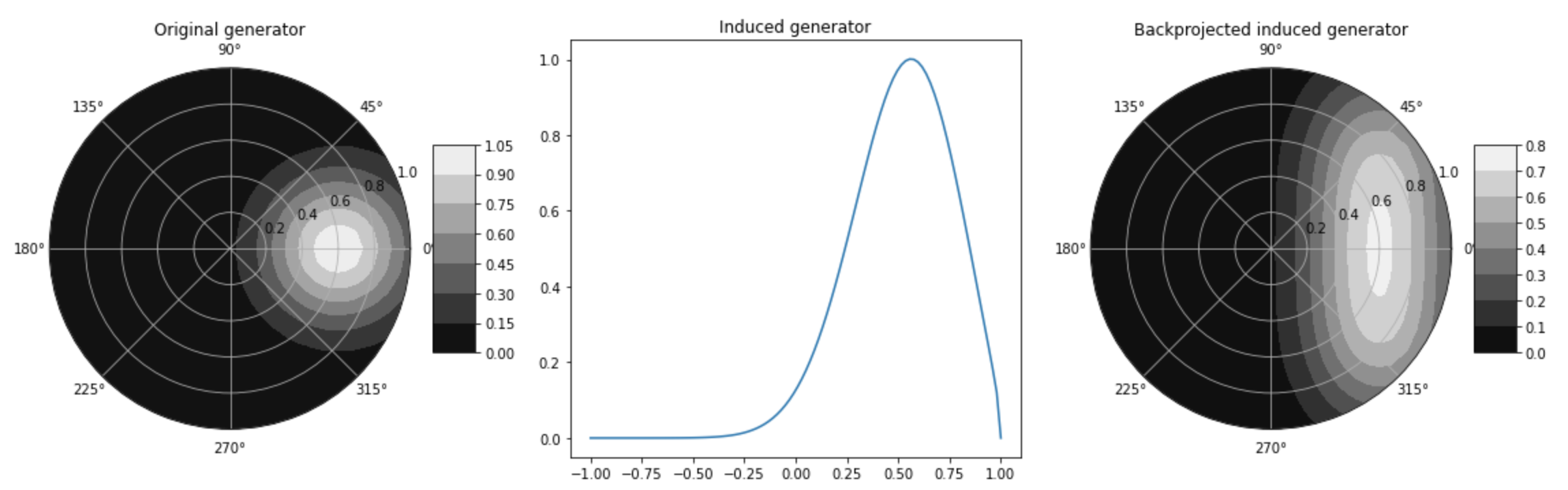
Figure 2: Gaussian kernel $K:\mathbb{B}^{2}\times\mathbb{B}^{2}\rightarrow\mathbb{R},(\mathbf{z}_{1},\mathbf{z}_{2})\mapsto\exp(-\gamma\|\mathbf{z}_{1}-\mathbf{z}_{2}\|^{2})$ with $\gamma=6$, used to plot three images: the original generator $k_{\mathbf{z}}:\mathbb{B}^{2}\rightarrow\mathbb{R}$ evaluated at $\mathbf{z}=(0.6,0)$, the induced generator $\tilde{k}^{R}_{\mathbf{x}}:\mathbb{B}\rightarrow\mathbb{R}$ evaluated at $\mathbf{x}=0.6$ and $R=I$, and its RKHS backprojection $\mathscr{P}_{R}^{*}(\tilde{k}^{R}_{\mathbf{x}}):\mathbb{B}^{2}\rightarrow\mathbb{R}$ evaluated at $\mathbf{x}=0.6$ and $R=I$, respectively.

As the adjoint operator $\mathscr{P}_{R}^{*}$ takes a function defined on $\mathbb{B}^{n-1}$ and smears over $\mathbb{B}^{n}$ to produce an a function defined on $\mathbb{B}^{n}$, we call it the kernel backprojection from this point onward, to distinguish from the usual backprojection in the $\mathcal{L}_{2}$ setting. In the $\mathcal{L}_{2}$ setting, $\mathscr{P}_{R}\circ\mathscr{P}_{R}^{*}$ does not result in the identity operator, necessitating the use of pre-filtering. In contrast, within the RKHS framework, we draw a natural analogy with the Euclidean projection in Proposition 2.1: the kernel backprojection $\mathscr{P}_{R}^{*}$ is an isometry, which might be interpreted as a smoothness-preserving operator, and it serves as the right inverse of the X-ray transform $\mathscr{P}_{R}$. Furthermore, although the reconstruction is an ill-posed problem in both the $\mathcal{L}_{2}$ and the RKHS framework, (6) demonstrates that the kernel backprojection generates the $n$-dimensional image of minimal norm among the solution set $\left\{f\in\mathbb{H}(K):g=\mathscr{P}_{R}f\right\}$.

3.2 Kernel Decomposition

To derive a representer theorem for the reconstruction in the following subsection, we introduce the decomposition of $\mathbb{H}(K)$ relevant to the discrete setup. Given limited access to the sinogram, in the form of finitely many projection images at orientations (say) $\mathbf{R}:=\{R_{i}\in SO(n):\ i=1,2,\dots,N\}$ (e.g. Fig. 1, right side), we aim to reconstruct the complete sinogram and the original $n$-dimensional structure $f^{0}\in\mathbb{H}(K)$. Let $\mathbf{F}:=\{\mathbf{x}_{1},\dots,\mathbf{x}_{M}\}\subset\mathbb{B}^{n-1}$ denote the mesh where the transformed images $g_{i}=\mathscr{P}_{R_{i}}f^{0}+W_{i}$ are evaluated under the presence of independent white noise $W_{i}$ in $\mathbb{H}(\tilde{K}^{R_{i}})$ of variance $\sigma^{2}>0$. Consequently, our observations are given by

$$y_{ij}:=g_{i}(\mathbf{x}_{j})=\mathscr{P}_{R_{i}}f^{0}(\mathbf{x}_{j})+\varepsilon_{ij},\quad 1\leq i\leq N,\ 1\leq j\leq M,$$

where $\varepsilon_{ij}:=W_{i}(\mathbf{x}_{j})$ are i.i.d. $N(0,\sigma^{2})$.

Proposition 3.5.

For any $R\in SO(n)$, let $\mathbb{V}_{\mathbf{F}}(\tilde{K}^{R}):=\operatorname*{span}\{\tilde{k}^{R}_{\mathbf{x}_{1}},\tilde{k}^{R}_{\mathbf{x}_{2}},\dots,\tilde{k}^{R}_{\mathbf{x}_{n}}\}$ denote the subspace of $\mathbb{H}(\tilde{K}^{R})$ spanned by the induced generators at mesh points.

1. $\mathscr{P}_{R}f(\mathbf{x}_{k})=0$ for all $k=1,\dots,M$ if and only if $f\in\mathscr{P}^{-1}_{R}((\mathbb{V}_{\mathbf{F}}(\tilde{K}^{R}))^{\perp})$.

2. $\mathscr{P}^{-1}_{R}((\mathbb{V}_{\mathbf{F}}(\tilde{K}^{R}))^{\perp})=\mathscr{P}_{R}^{*}((\mathbb{V}_{\mathbf{F}}(\tilde{K}^{R}))^{\perp})\oplus\mathcal{N}(\mathscr{P}_{R})$ is a closed subspace of $\mathbb{H}(K)$.

3. $(\mathscr{P}^{-1}_{R}((\mathbb{V}_{\mathbf{F}}(\tilde{K}^{R}))^{\perp}))^{\perp}=\mathscr{P}_{R}^{*}(\mathbb{V}_{\mathbf{F}}(\tilde{K}^{R}))$ is a closed subspace of $\mathbb{H}(K)$.

Owing to the proposition above, we get an elegant decomposition of the domain $\mathbb{H}(K)$ for any $R\in SO(n)$:

$$\mathbb{H}(K) =\mathscr{P}_{R}^{*}(\mathbb{V}_{\mathbf{F}}(\tilde{K}^{R})) \oplus\mathscr{P}_{R}^{*}((\mathbb{V}_{\mathbf{F}}(\tilde{K}^{R}))^{\perp}) \oplus\,\mathcal{N}(\mathscr{P}_{R}),$$ (7)

$$f =\quad f_{\mathbf{F}}^{R} \oplus\,(\mathscr{P}^{*}_{R}\mathscr{P}_{R}f-f_{\mathbf{F}}^{R}) \oplus\,(f-\mathscr{P}^{*}_{R}\mathscr{P}_{R}f),$$

where $f_{\mathbf{F}}^{R}:=\sum_{j=1}^{M}\alpha_{j}\mathscr{P}^{*}_{R}\tilde{k}_{\mathbf{x}_{j}}^{R}$ is uniquely determined by the linear system:

$$\mathscr{P}_{R}f(\mathbf{x}_{j})=\mathscr{P}_{R}f_{\mathbf{F}}^{R}(\mathbf{x}_{j})=\sum_{j^{\prime}=1}^{M}\alpha_{j^{\prime}}\tilde{K}^{R}(\mathbf{x}_{j},\mathbf{x}_{j^{\prime}}),\quad j=1,\dots,M.$$ (8)

The unidentifiable nature of the component in $\mathcal{N}(\mathscr{P}_{R})$ in (7) persists irrespective of the mesh points used. On the other hand, the identifiability (or lack thereof) of $\mathscr{P}_{R}^{*}((\mathbb{V}_{\mathbf{F}}(\tilde{K}^{R}))^{\perp})$ is dependent on the selected grid. Lastly, as evident from (8), the dimension of the identifiable component, $\mathscr{P}_{R}^{*}(\mathbb{V}_{\mathbf{F}}(\tilde{K}^{R}))$, does not exceed the number of mesh points used in the reconstruction.

For subspaces $\mathbb{V}_{1},\dots,\mathbb{V}_{N}$ in $\mathbb{H}(K)$, we denote the sum of subspaces by $\mathop{\mathchoice{\vbox{\hbox{\leavevmode\resizebox{}{9.00005pt}{\raisebox{0.0pt}{$\displaystyle+$}}}}\vphantom{\sum}}{\vbox{\hbox{\leavevmode\resizebox{}{9.00005pt}{\raisebox{0.0pt}{$\textstyle+$}}}}\vphantom{\sum}}{\vbox{\hbox{\leavevmode\resizebox{}{6.30003pt}{\raisebox{0.0pt}{$\scriptstyle+$}}}}\vphantom{\sum}}{\vbox{\hbox{\leavevmode\resizebox{}{4.50002pt}{\raisebox{0.0pt}{$\scriptscriptstyle+$}}}}\vphantom{\sum}}}\slimits@_{i=1}^{N}\mathbb{V}_{i}:=\{\sum_{i=1}^{N}v_{i}:v_{1}\in\mathbb{V}_{1},\dots,v_{N}\in\mathbb{V}_{N}\}$. When $\mathbb{V}_{1},\dots,\mathbb{V}_{N}$ are closed subspaces, then $(\bigcap_{i=1}^{N}\mathbb{V}_{i})^{\perp}=\overline{\mathbb{V}_{1}^{\perp}+\dots+\mathbb{V}_{N}^{\perp}}$. Hence, for multiple orientations $\mathbf{R}=\{R_{i}\in SO(n):\ i=1,2,\dots,N\}$, (7) becomes

$$\mathbb{H}(K)=\left(\mathop{\mathchoice{\vbox{\hbox{\leavevmode\resizebox{}{9.00005pt}{\raisebox{0.0pt}{$\displaystyle+$}}}}\vphantom{\sum}}{\vbox{\hbox{\leavevmode\resizebox{}{9.00005pt}{\raisebox{0.0pt}{$\textstyle+$}}}}\vphantom{\sum}}{\vbox{\hbox{\leavevmode\resizebox{}{6.30003pt}{\raisebox{0.0pt}{$\scriptstyle+$}}}}\vphantom{\sum}}{\vbox{\hbox{\leavevmode\resizebox{}{4.50002pt}{\raisebox{0.0pt}{$\scriptscriptstyle+$}}}}\vphantom{\sum}}}\slimits@_{i=1}^{N}\mathscr{P}^{*}_{R_{i}}(\mathbb{V}_{\mathbf{F}}(\tilde{K}^{R_{i}}))\right)\oplus\left(\bigcap_{i=1}^{N}\mathscr{P}^{-1}_{R_{i}}((\mathbb{V}_{\mathbf{F}}(\tilde{K}^{R_{i}}))^{\perp})\right).$$ (9)

Let $\mathbb{H}^{\mathbf{R}}_{\mathbf{F}}:=\mathop{\mathchoice{\vbox{\hbox{\leavevmode\resizebox{}{9.00005pt}{\raisebox{0.0pt}{$\displaystyle+$}}}}\vphantom{\sum}}{\vbox{\hbox{\leavevmode\resizebox{}{9.00005pt}{\raisebox{0.0pt}{$\textstyle+$}}}}\vphantom{\sum}}{\vbox{\hbox{\leavevmode\resizebox{}{6.30003pt}{\raisebox{0.0pt}{$\scriptstyle+$}}}}\vphantom{\sum}}{\vbox{\hbox{\leavevmode\resizebox{}{4.50002pt}{\raisebox{0.0pt}{$\scriptscriptstyle+$}}}}\vphantom{\sum}}}\slimits@_{i=1}^{N}\mathscr{P}^{*}_{R_{i}}(\mathbb{V}_{\mathbf{F}}(\tilde{K}^{R_{i}}))=\text{span}\{\mathscr{P}^{*}_{R_{i}}\tilde{k}_{\mathbf{x}_{j}}^{R_{i}}:1\leq i\leq N,1\leq j\leq M\}$, a subspace of $\mathbb{H}(K)$ with dimension at most $NM$, and define $\mathcal{P}_{\mathbf{F}}^{\mathbf{R}}:\mathbb{H}(K)\rightarrow\mathbb{H}^{\mathbf{R}}_{\mathbf{F}}$ to be the projection operator onto $\mathbb{H}^{\mathbf{R}}_{\mathbf{F}}$. Proposition 3.5 part (1) reveals that the evaluation of the projected image solely depends on $\mathcal{P}_{\mathbf{F}}^{\mathbf{R}}f$, i.e.

$$\mathscr{P}_{R_{i}}f(\mathbf{x}_{j})=(\mathscr{P}_{R_{i}}\circ\mathcal{P}_{\mathbf{F}}^{\mathbf{R}})f(\mathbf{x}_{j}),\quad 1\leq i\leq N,\ 1\leq j\leq M.$$ (10)

Again, when we observe projection images from angles $R_{1},\dots,R_{N}$ with the mesh points $\mathbf{x}_{1},\dots,\mathbf{x}_{M}$, it is impossible to extract any information about the image component that belongs to $(\mathbb{H}^{\mathbf{R}}_{\mathbf{F}})^{\perp}$. The best we can do is to estimate

$$\mathcal{P}_{\mathbf{F}}^{\mathbf{R}}f=\sum_{i=1}^{N}\sum_{j=1}^{M}\alpha_{ij}\mathscr{P}^{*}_{R_{i}}\tilde{k}_{\mathbf{x}_{j}}^{R_{i}}.$$

To introduce the representer theorem, we establish some notation. We define the vectorization of $\alpha_{ij}$ and the weight matrix, respectively, as

$$\boldsymbol{\alpha}:=\mathrm{vec}[\alpha_{ij}]\in\mathbb{R}^{NM},$$

$$\mathbf{W}:=\left[w_{ij,i^{\prime}j^{\prime}}=\langle\mathscr{P}_{R_{i}}^{*}\tilde{k}^{R_{i}}_{\mathbf{x}_{j}},\mathscr{P}_{R_{i^{\prime}}}^{*}\tilde{k}^{R_{i^{\prime}}}_{\mathbf{x}_{j^{\prime}}}\rangle_{\mathbb{H}(K)}\right]\in\mathbb{R}^{NM\times NM}.$$

The Gram matrix $\mathbf{W}$ is clearly positive semidefinite. Additionally, due to (5), we have an equivalent expression for $w_{ij,i^{\prime}j^{\prime}}\in\mathbb{R}$:

$$w_{ij,i^{\prime}j^{\prime}} =\langle\mathscr{P}_{R_{i}}^{*}\tilde{k}^{R_{i}}_{\mathbf{x}_{j}},\mathscr{P}_{R_{i^{\prime}}}^{*}\tilde{k}^{R_{i^{\prime}}}_{\mathbf{x}_{j^{\prime}}}\rangle_{\mathbb{H}(K)}=(\mathscr{P}_{R_{i}}\circ\mathscr{P}_{R_{i^{\prime}}}^{*}\tilde{k}^{R_{i^{\prime}}}_{\mathbf{x}_{j^{\prime}}})(\mathbf{x}_{j})$$ (11)

$$=\int_{I_{\|\mathbf{x}_{j^{\prime}}\|}}\int_{I_{\|\mathbf{x}_{j}\|}}K(R_{i}^{\top}[\mathbf{x}_{j}:z_{1}],R_{i^{\prime}}^{\top}[\mathbf{x}_{j^{\prime}}:z_{2}])\mathrm{d}z_{1}\mathrm{d}z_{2}.$$

Proposition 3.6.

The projection $\mathcal{P}_{\mathbf{F}}^{\mathbf{R}}f=\sum_{i=1}^{N}\sum_{j=1}^{M}\alpha_{ij}\mathscr{P}^{*}_{R_{i}}\tilde{k}_{\mathbf{x}_{j}}^{R_{i}}$ of $f\in\mathbb{H}(K)$ onto $\mathbb{H}^{\mathbf{R}}_{\mathbf{F}}$ is uniquely determined by the linear system:

$$\mathrm{vec}[\mathscr{P}_{R_{i}}f(\mathbf{x}_{j})]=\mathrm{vec}[(\mathscr{P}_{R_{i}}\circ\mathcal{P}_{\mathbf{F}}^{\mathbf{R}})f(\mathbf{x}_{j})]=\mathbf{W}\boldsymbol{\alpha}\in\mathbb{R}^{NM}.$$

Denote by $\mathcal{R}(\mathbf{W})$ the range space of the Gram matrix $\mathbf{W}$, equipped with the inner product $\langle\mathbf{W}\alpha,\mathbf{W}\beta\rangle_{\mathbf{W}}=\alpha^{\top}\mathbf{W}\beta$. Then, the map

$$\mathcal{I}^{\mathbf{R}}_{\mathbf{F}}:(\mathbb{H}^{\mathbf{R}}_{\mathbf{F}},\langle\cdot,\cdot\rangle_{\mathbb{H}(K)})\rightarrow(\mathcal{R}(\mathbf{W}),\langle\cdot,\cdot\rangle_{\mathbf{W}}),\ \sum_{i=1}^{N}\sum_{j=1}^{M}\alpha_{ij}\mathscr{P}^{*}_{R_{i}}\tilde{k}_{\mathbf{x}_{j}}^{R_{i}}\mapsto\mathbf{W}\boldsymbol{\alpha}$$ (12)

is an isomorphism Furthermore, if the kernel $K:\mathbb{B}^{n}\times\mathbb{B}^{n}\rightarrow\mathbb{R}$ is strictly p.d. and $\mathbf{F}=\{\mathbf{x}_{1},\dots,\mathbf{x}_{M}\}\subset(\mathbb{B}^{n-1})^{\circ}$, then $\mathbf{W}\in\mathbb{R}^{NM\times NM}$ is also strictly p.d., thus $\dim(\mathbb{H}^{\mathbf{R}}_{\mathbf{F}})=\dim(\mathbf{W})=NM$.

Remark 3.7.

With regards to implementation, we inscribe the pixelated projected images in the unit ball $\mathbb{B}^{n-1}$ and register coordinates $\mathbf{F}=\{\mathbf{x}_{j}:j=1,\dots,M\}$ to each pixel. If a pixel is matched to a point on the boundary, say $\mathbf{x}_{1}\in\partial\mathbb{B}^{n-1}$, it is virtually the same as neglecting the corresponding pixel. The weights $w_{ij,i^{\prime}j^{\prime}}$ in (11) will be zero whenever $j=1$ or $j^{\prime}=1$, resulting in entirely zero columns and rows within the weight matrix $\mathbf{W}$, which renders $\mathbf{W}$ non-invertible, while its Moore-Penrose inverse is equivalent to that of $\mathbf{F}-\{x_{1}\}$. For strictly p.d. kernels, the singularity of $\mathbf{W}$ is not tied to inherent relationships between mesh points, but rather to whether $\mathbf{F}\cap\partial\mathbb{B}^{n-1}=\emptyset$ or not. In conclusion, it is prudent to avoid situating a mesh point on the boundary, as such a point jeopardizes computational stability without playing any role.

3.3 Kernel Reconstruction

We now consider the reconstruction problem, adopting a (penalized) Maximum Likelihood Estimator (MLE) approach within the RKHS framework. This reduces reconstruction to a linear regression problem. Recall that our observations are

$$y_{ij}=\mathscr{P}_{R_{i}}f^{0}(\mathbf{x}_{j})+\varepsilon_{ij},\quad i=1,2,\dots,N,\,j=1,2,\dots,M,$$

where $\varepsilon_{ij}=W_{i}(\mathbf{x}_{j})$ are i.i.d. $N(0,\sigma^{2})$. Hence, an MLE satisfies

$$\hat{f}^{0}\ \in \ \operatorname*{\arg\max}_{f\in\mathbb{H}(K)}\prod_{i=1}^{N}\prod_{j=1}^{M}\frac{1}{\sqrt{2\pi}\sigma}\exp\left(-\frac{(y_{ij}-\mathscr{P}_{R_{i}}f^{0}(\mathbf{x}_{j}))^{2}}{2\sigma^{2}}\right)=\operatorname*{\arg\min}_{f\in\mathbb{H}(K)}\hat{L}^{0}(f),$$

where the empirical risk functional

$$\hat{L}^{0}(f):=\sum_{i=1}^{N}\sum_{j=1}^{M}\left(y_{ij}-\mathscr{P}_{R_{i}}f(\mathbf{x}_{j})\right)^{2},$$

is associated with the risk functional $L^{0}(f):=\sum_{i=1}^{N}\sum_{j=1}^{M}\mathbb{E}[\left(y_{ij}-\mathscr{P}_{R_{i}}f(\mathbf{x}_{j})\right)^{2}]$. Denote by $\mathbf{Y}:=\mathrm{vec}[y_{ij}]\in\mathbb{R}^{NM},\ \boldsymbol{\alpha}^{0}:=\mathrm{vec}[\alpha^{0}_{ij}]\in\mathbb{R}^{NM}$ the vectorizations of $y_{ij},\alpha^{0}_{ij}$, where $\mathcal{P}_{\mathbf{F}}^{\mathbf{R}}f^{0}=\sum_{i=1}^{N}\sum_{j=1}^{M}\alpha^{0}_{ij}\mathscr{P}^{*}_{R_{i}}\tilde{k}_{\mathbf{x}_{j}}$. Using the vectorization, the risk functionals become

$$\hat{L}^{0}(f)=\hat{L}^{0}(\mathcal{P}_{\mathbf{F}}^{\mathbf{R}}f)=\hat{L}^{0}(\boldsymbol{\alpha})=\|\mathbf{Y}-\mathbf{W}\boldsymbol{\alpha}\|^{2},$$

$$L^{0}(f)=L^{0}(\mathcal{P}_{\mathbf{F}}^{\mathbf{R}}f)=L^{0}(\boldsymbol{\alpha})=\|\mathbf{W}\boldsymbol{\alpha}^{0}-\mathbf{W}\boldsymbol{\alpha}\|^{2}+NM\sigma^{2}.$$

Therefore, we recover the following normal equation:

$$\mathbf{W}^{2}\hat{\boldsymbol{\alpha}}^{0}=\mathbf{W}\mathbf{Y}\quad \Longleftrightarrow\quad\mathbf{W}\hat{\boldsymbol{\alpha}}^{0}=\mathbf{W}\mathbf{W}^{\dagger}\mathbf{Y}$$ (13)

$$\Longleftrightarrow\quad\mathcal{P}_{\mathbf{F}}^{\mathbf{R}}\hat{f}^{0}=(\mathcal{I}^{\mathbf{R}}_{\mathbf{F}})^{-1}(\mathbf{W}\hat{\boldsymbol{\alpha}}^{0})=(\mathcal{I}^{\mathbf{R}}_{\mathbf{F}})^{-1}(\mathbf{W}\mathbf{W}^{\dagger}\mathbf{Y}).$$

It is worthwhile to highlight the logical pathway through which we can derive the classical least square estimation for the reconstruction. As indicated in (10), given $R_{1},\dots,R_{N}$ with the mesh points $\mathbf{x}_{1},\dots,\mathbf{x}_{M}$, we cannot identify components that belong to $(\mathbb{H}^{\mathbf{R}}_{\mathbf{F}})^{\perp}$. As a result, instead of $\mathbb{H}(K)$, the de facto space we are working on is $(\mathbb{H}^{\mathbf{R}}_{\mathbf{F}},\langle\cdot,\cdot\rangle_{\mathbb{H}(K)})\cong(\mathcal{R}(\mathbf{W}),\langle\cdot,\cdot\rangle_{\mathbf{W}})$, as outlined in (12).

Theorem 3.8 (X-ray Linear Regression).

Let $\mathbf{R}=\{R_{1},\dots,R_{N}\}\subset SO(n)$ be viewing angles and $\mathbf{F}=\{\mathbf{x}_{1},\dots,\mathbf{x}_{M}\}\subset\mathbb{B}^{n-1}$ be an evaluating grid. Also, let $\mathcal{I}^{\mathbf{R}}_{\mathbf{F}}:(\mathbb{H}^{\mathbf{R}}_{\mathbf{F}},\langle\cdot,\cdot\rangle_{\mathbb{H}(K)})\rightarrow(\mathcal{R}(\mathbf{W}),\langle\cdot,\cdot\rangle_{\mathbf{W}})$ be the isomorphism defined as in (12).

1. Let $\hat{\boldsymbol{\alpha}}^{0}:=\mathbf{W}^{\dagger}\mathbf{Y}\in\mathcal{R}(\mathbf{W})$ and $\hat{f}^{0}:=\sum_{i=1}^{N}\sum_{j=1}^{M}\hat{\alpha}^{0}_{ij}\mathscr{P}^{*}_{R_{i}}\tilde{k}_{\mathbf{x}_{j}}\in\mathbb{H}^{\mathbf{R}}_{\mathbf{F}}$. Then,

   $$\operatorname*{\arg\min}_{f\in\mathbb{H}(K)}\hat{L}^{0}(f)=\hat{f}^{0}\oplus(\mathbb{H}^{\mathbf{R}}_{\mathbf{F}})^{\perp},$$

   i.e. $\hat{f}^{0}$ is the minimizer of $\hat{L}^{0}$ with minimum norm.

2. $\operatorname*{\arg\min}_{f\in\mathbb{H}(K)}L^{0}(f)=\mathcal{P}_{\mathbf{F}}^{\mathbf{R}}f^{0}\oplus(\mathbb{H}^{\mathbf{R}}_{\mathbf{F}})^{\perp}$, i.e. $\mathcal{P}_{\mathbf{F}}^{\mathbf{R}}f^{0}$ is the minimizer of $L^{0}$ with minimum norm.

3. $\hat{\boldsymbol{\alpha}}^{0}\sim N(\mathbf{W}\mathbf{W}^{\dagger}\boldsymbol{\alpha}^{0},\sigma^{2}(\mathbf{W}^{\dagger})^{2})$, $\hat{f}^{0}\sim N(\mathcal{P}_{\mathbf{F}}^{\mathbf{R}}f^{0},\sigma^{2}(\mathcal{I}^{\mathbf{R}}_{\mathbf{F}})^{-1}\circ\mathbf{W}^{\dagger}\circ(\mathcal{I}^{\mathbf{R}}_{\mathbf{F}}))$, where $\mathbf{W}^{\dagger}$ is the Moore-Penrose inverse of $\mathbf{W}$.

Our regression setting differs from the traditional $\mathcal{L}_{2}$ setting. Methods based on the SVD of the compact operator $\mathscr{P}:\mathcal{L}_{2}(\mathbb{B}^{n})\rightarrow\mathcal{L}_{2}(SO(n)\times\mathbb{B}^{n-1},W^{-1})$ typically fix the choice of basis as the singular vectors, taking the form of $f_{mlk}(r\theta)=Z_{ml}(r)Y_{lk}(\theta)$, where the radial basis $Z_{ml}$ consists of Zernike polynomials, and $Y_{lk}$ represents spherical harmonics [20, 18]. However, in our framework:

1. The MLE $\hat{f}^{0}$ can vary based on the selection of the kernel $K:\mathbb{B}^{n}\times\mathbb{B}^{n}\rightarrow\mathbb{R}$, granting us more flexibility in selecting a basis.

2. The rank of the design matrix $\mathbf{W}$ is not determined by the truncation level, but by the total number of observations $NM$.

Arguably, our reconstruction method represents a more general framework than the truncated SVD, as the latter corresponds to a specific choice of non-strictly p.d. kernels. For further details, we refer to the discussion following Remark 4.10.

The design matrix $\mathbf{W}$ is always square by construction, so there is no parsimony at play here. In Proposition 3.6, we demonstrate that when using a strictly positive definite kernel with interior mesh points $\mathbf{F}=\{\mathbf{x}_{1},\dots,\mathbf{x}_{M}\}\subset(\mathbb{B}^{n-1})^{\circ}$, $\mathbf{W}$ becomes full rank, i.e., $\mathcal{R}(\mathbf{W})=\mathbb{R}^{NM}$. Consequently, the MLE $\hat{f}^{0}$ generates a sinogram that perfectly interpolates our observations $\mathbf{Y}=\mathrm{vec}[y_{ij}]\in\mathbb{R}^{NM}$ regardless of the presence of the noise, i.e. $\min_{f\in\mathbb{H}(K)}\hat{L}^{0}(f)=\min_{\boldsymbol{\alpha}\in\mathbb{R}^{MN}}\hat{L}^{0}(\boldsymbol{\alpha})=0$. To address this issue of overfitting, we consider Tikhonov regularization, leading to a penalized MLE. For a tuning parameter $\nu>0$, we introduce a penalty term to the empirical risk functional $\hat{L}^{\nu}:\mathbb{H}(K)\rightarrow\mathbb{R}$ as follows:

$$\hat{L}^{\nu}(f)=\sum_{i=1}^{N}\sum_{j=1}^{M} \left(y_{ij}-\mathscr{P}_{R_{i}}f(\mathbf{x}_{j})\right)^{2}+\nu\|f\|^{2}_{\mathbb{H}(K)}.$$

Due to (10) , we have $\hat{L}^{\nu}(f)\geq\hat{L}^{\nu}(\mathcal{P}_{\mathbf{F}}^{\mathbf{R}}f)$, hence any minimizer $\hat{f}^{\nu}$ of the penalized risk $\hat{L}^{\nu}$ belongs to $\mathbb{H}^{\mathbf{R}}_{\mathbf{F}}$, i.e. there are some $\hat{\alpha}^{\nu}_{ij}$ such that $\hat{f}^{\nu}=\mathcal{P}_{\mathbf{F}}^{\mathbf{R}}\hat{f}^{\nu}=\sum_{i=1}^{N}\sum_{j=1}^{M}\hat{\alpha}^{\nu}_{ij}\mathscr{P}^{*}_{R_{i}}\tilde{k}^{R_{i}}_{\mathbf{x}_{j}}$. By Proposition 3.6, the empirical risk functional becomes

$$\hat{L}^{\nu}(f)\geq\hat{L}^{\nu}(\mathcal{P}_{\mathbf{F}}^{\mathbf{R}}f)=\|\mathbf{Y}-\mathbf{W}\boldsymbol{\alpha}\|^{2}+\nu\boldsymbol{\alpha}^{\top}\mathbf{W}\boldsymbol{\alpha},$$

which yields the normal equation as follows:

$$(\mathbf{W}^{2}+\nu\mathbf{W})\hat{\boldsymbol{\alpha}}^{\nu}=\mathbf{W}\mathbf{Y}\, \Longleftrightarrow\,\mathbf{W}\hat{\boldsymbol{\alpha}}^{\nu}=\mathbf{W}(\mathbf{W}+\nu\mathbf{I})^{-1}\mathbf{Y}.$$ (14)

In summary, we deduce the representer theorem below for the regularized reconstruction. We also highlight that, whenever the penalty function is a strictly monotone increasing function of $\|f\|_{\mathbb{H}(K)}$, the same argument remains valid: the minimizer belongs to $\mathbb{H}_{\mathbf{F}}^{\mathbf{R}}$. Additionally, if the penalty function is also convex, then the minimizer is unique.

Theorem 3.9 (Tikhonov Kernel Reconstruction).

Let $\mathbf{R}=\{R_{1},\dots,R_{N}\}\subset SO(n)$ be viewing angles, $\mathbf{F}=\{\mathbf{x}_{1},\dots,\mathbf{x}_{M}\}\subset\mathbb{B}^{n-1}$ be an evaluating grid, and $\nu>0$ be a regularization parameter. Also, let $\mathcal{I}^{\mathbf{R}}_{\mathbf{F}}:(\mathbb{H}^{\mathbf{R}}_{\mathbf{F}},\langle\cdot,\cdot\rangle_{\mathbb{H}(K)})\rightarrow(\mathcal{R}(\mathbf{W}),\langle\cdot,\cdot\rangle_{\mathbf{W}})$ be the isomorphism defined as in (12).

1. The unique minimizer of $\hat{L}^{\nu}(f)$ is given by $\hat{f}^{\nu}=\sum_{i=1}^{N}\sum_{j=1}^{M}\hat{\alpha}^{\nu}_{ij}\mathscr{P}^{*}_{R_{i}}\tilde{k}^{R_{i}}_{\mathbf{x}_{j}}\in\mathbb{H}^{\mathbf{R}}_{\mathbf{F}}$, where $\hat{\boldsymbol{\alpha}}^{\nu}:=(\mathbf{W}+\nu\mathbf{I})^{-1}\mathbf{Y}$.

2. The minimum of the empirical risk is given by

   $$\min_{f\in\mathbb{H}(K)}\hat{L}^{\nu}(f)=\min_{\boldsymbol{\alpha}\in\mathbb{R}^{MN}}\hat{L}^{\nu}(\boldsymbol{\alpha})=\hat{L}^{\nu}(\hat{\boldsymbol{\alpha}}^{\nu})=\nu\mathbf{Y}^{\top}(\mathbf{W}+\nu\mathbf{I})^{-1}\mathbf{Y}.$$

3. $\hat{\boldsymbol{\alpha}}^{\nu}\sim N(\mathbf{W}(\mathbf{W}+\nu\mathbf{I})^{-1}\boldsymbol{\alpha}^{0},\sigma^{2}(\mathbf{W}+\nu\mathbf{I})^{-2})$ and $\hat{f}^{\nu}$ is the finite-dimensional degenerate Gaussian process:

   $$\hat{f}^{\nu}\sim N((\mathcal{I}^{\mathbf{R}}_{\mathbf{F}})^{-1}(\mathbf{W}^{2}(\mathbf{W}+\nu\mathbf{I})^{-1}\boldsymbol{\alpha}^{0}),\sigma^{2}(\mathcal{I}^{\mathbf{R}}_{\mathbf{F}})^{-1}\circ(\mathbf{W}(\mathbf{W}+\nu\mathbf{I})^{-2})\circ(\mathcal{I}^{\mathbf{R}}_{\mathbf{F}})).$$

4. As $\nu\downarrow 0$, $\hat{\boldsymbol{\alpha}}^{\nu}$ and $\hat{f}^{\nu}$ converge to the MLEs $\hat{\boldsymbol{\alpha}}^{0}$ and $\hat{f}^{0}$ in $\mathbb{R}^{NM}$ and $\mathbb{H}(K)$, respectively: $\lim_{\nu\downarrow 0}\hat{\boldsymbol{\alpha}}^{\nu}=\hat{\boldsymbol{\alpha}}^{0},\ \lim_{\nu\downarrow 0}\hat{f}^{\nu}=\hat{f}^{0}$.

Our X-ray representer theorem produces a reconstructed image at a funcitonal level within the discrete setup. This reconstruction bypasses the projection image interpolation step, as it automatically satisfies the consistency condition in Theorem 2.9:

Proposition 3.10.

The Tikhonov regularized reconstruction in Theorem 3.9 produces an interpolation of the projection images as follows: for any $R\in SO(n)$ and $\mathbf{x}\in\mathbb{B}^{n-1}$,

$$\mathscr{P}\hat{f}^{\nu}(R,\mathbf{x})=\langle\mathscr{P}_{R}^{*}\tilde{k}^{R}_{\mathbf{x}},\hat{f}^{\nu}\rangle_{\mathbb{H}(K)}=\sum_{i=1}^{N}\sum_{j=1}^{M}\hat{\alpha}^{\nu}_{ij}\langle\mathscr{P}_{R}^{*}\tilde{k}^{R}_{\mathbf{x}},\mathscr{P}_{R_{i}}^{*}\tilde{k}^{R_{i}}_{\mathbf{x}_{j}}\rangle_{\mathbb{H}(K)}.$$

Furthermore, the interpolant $\mathscr{P}\hat{f}^{\nu}\in\mathbb{H}(\tilde{K}^{R})$ is a bona fide sinogram, i.e. it satisfies the HLCC in Theorem 2.9: for any $l\in\mathbb{Z}_{+}$, we have

$$\int_{\mathbb{B}^{n-1}}(\mathbf{x}^{\top}\mathbf{y})^{l}\mathscr{P}\hat{f}^{\nu}(R,\mathbf{x})\mathrm{d}\mathbf{x}=q_{l}^{\nu}(\mathbf{P}_{R}^{*}(\mathbf{y})),\quad\mathbf{y}\in\mathbb{R}^{n-1},$$

where $q_{l}^{\nu}(\cdot):=\int_{\mathbb{B}^{n}}(\mathbf{z}^{\top}\cdot)^{l}\hat{f}^{\nu}(\mathbf{z})\mathrm{d}\mathbf{z}$ is a homogeneous polynomial of degree $l$, independent of $R\in SO(n)$.

3.4 Stability

Reconstruction stability is influenced by two primary sources of error. The first source is obviously measurement errors, and several stability inequalities have been established in terms of $\|\mathscr{P}(f-f^{0})\|$ and $\|f^{0}\|$ under some regularity conditions [23, 20]. These results prove valuable only if we have access to an entire perturbed sinogram. However, our situation involves only a finite number of discretized projection images, which in effect constitutes a second error source. In this discrete setup, previous studies [18, 20] have addressed the issue of resolution, i.e. characterizing the degree of oscillation in reconstructed images. Nonetheless, to the best of our knowledge, there exists no stability inequality that specifically addresses the discretized measurement error. To bridge this gap, we establish a sharp stability result for our algorithm, in the realistic setting of discretized measurements corrupted by errors, in two setups: random errors of given variance, Proposition 3.11, and deterministic errors with given bounded norm, Theorem 3.12.

Proposition 3.11.

The mean squared error of the Tikhonov regularizer with tuning parameter $\nu>0$ in Theorem 3.9 is given by

MSE $$(\hat{f}^{\nu}):=\mathbb{E}[\|\hat{f}^{\nu}-f^{0}\|^{2}_{\mathbb{H}(K)}]$$

$$= \nu^{2}(\boldsymbol{\alpha}^{0})^{\top}\mathbf{W}(\mathbf{W}+\nu\mathbf{I})^{-2}\boldsymbol{\alpha}^{0}+\sigma^{2}\text{tr}(\mathbf{W}(\mathbf{W}+\nu\mathbf{I})^{-2})+\|f^{0}-\mathcal{P}_{\mathbf{F}}^{\mathbf{R}}f^{0}\|^{2}_{\mathbb{H}(K)}.$$

Theorem 3.12.

Let be $\nu>0$ a tuning parameter, and $d>0$ be the smallest non-zero eigenvalue of the Gram matrix $\mathbf{W}\in\mathbb{R}^{NM\times NM}$. Then, the worst-case squared error of the Tikhonov regularizer in Theorem 3.9 is given as follows:

$$\text{err}(\rho,\varepsilon):=\max\left\{\|\hat{f}^{\nu}-f^{0}\|^{2}_{\mathbb{H}(K)}:\|f^{0}\|_{\mathbb{H}(K)}\leq\rho,\,\sum_{i=1}^{N}\sum_{j=1}^{M}\varepsilon_{ij}^{2}\leq\varepsilon^{2}\right\}=\rho^{2}+\frac{\varepsilon^{2}}{d+2\nu}.$$

Remark 3.13.

The proof of Theorem 3.12 exemplifies the technical advantage of the RKHS framework. In the context of discrete setup, the RKHS framework has the ability to explicitly define the identifiable space $\mathbb{H}^{\mathbf{R}}_{\mathbf{F}}$, which is a finite-dimensional space. We can then apply a technique similar to demonstrating the shrinkage effect in ridge regression, allowing us to derive the sharp inequality.

The above theorem reveals the stabilizing effect of introducing a penalty term. Whereas $1/(d+2\nu)\approx 1/(2\nu)$ when $\nu\gg 1$, $1/(d+2\nu)\approx 1/d$ when $\nu\ll 1$. Hence, in cases where the dimension of the Gram matrix increases substantially, leading to a situation where the smallest non-zero eigenvalue $d>0$ approaches zero, the MLE in Theorem 3.8 may exhibit instability, see Fig. 7 in the appendix. We further remark that the above result also immediately yields pointwise stability since $|\hat{f}^{\nu}(\mathbf{z})-f^{0}(\mathbf{z})|^{2}\leq K(\mathbf{z},\mathbf{z})\|\hat{f}^{\nu}-f^{0}\|^{2}_{\mathbb{H}(K)}$ by the Cauchy-Schwarz inequality.

3.5 Illustrative Examples

We provide three illustrative examples in this section, with two additional scenarios covered in Appendix D. These scenarios serve to highlight the significant disparity between our Kernel Reconstruction (KR) approach and the conventional Filtered Backprojection (FBP) method. In our experiments, we use a 10-times intensified $M\times M$ ($M=200$) image of the 2D Shepp-Logan phantom as a benchmark for the original structure $f^{0}$. For FBP reconstruction, we apply a ramp filter for the filtering process. In our Tikhonov kernel reconstruction (Theorem 3.9), we employ a Gaussian kernel $K(\mathbf{z}_{1},\mathbf{z}_{2})=\exp\{-\gamma\|\mathbf{z}_{1}-\mathbf{z}_{2}\|^{2}\}$ with $\gamma=200$, and we set the penalty level to $\nu=0.1$.

There are two reasons to select the Gaussian kernel. First, it is a rotation-invariant kernel that allows rapid Gram matrix computations using the cumulative distribution function (CDF) of the standard bivariate normal distribution. This holds for any dimension $n\in\mathbb{N}$, as elaborated in Proposition A.3. Second, the Gaussian kernel is strictly p.d., and thus induces an infinite-dimensional RKHS, leading to a behaviour that is distinct (and arguably improved) compared to the FBP method, as discussed in Section 4.2.

In Fig. 3, we consider the noiseless sinogram with parallel geometry, i.e. $N=40$ angles equiangular over $[-\pi/2,\pi/2)$ (rad). As the Fourier transform is inherent in the FBP algorithm, it produces a highly oscillating reconstruction error across the whole image [20]. However, the KR algorithm renders a rather regularized and smooth image in order to balance a measure of goodness of fit. Consequently, the image is rather blurred and the trade-off between fidelity to the data and roughness of the function estimate can be clearly seen in the reconstruction error of the algorithm.

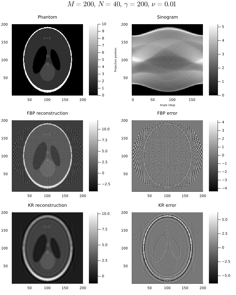
Figure 3: Reconstructions of an ideal sinogram (top right) at $N=40$ equidistant angles over $[-\pi/2,\pi/2)$ (rad), generated by the 10-times intensified, $M\times M$ ($M=200$) pixelated 2D Shepp-Logan phantom (top left). The Gaussian kernel with $\gamma=200$ and the penalty level $\nu=0.1$ in Theorem 3.9 was used for the kernel reconstruction (bottom left). The middle row is the FBP reconstruction with the ramp filter.

In adversarial situations with a high level of perturbation and irregular viewing angles as in Fig. 4, the FBP algorithm suffers from aliasing degradation caused by the discretization of the projection images [27]. In contrast, the KR reconstruction is less prone to producing artifacts. Even in cases with very low signal-to-noise ratio (SNR) ($\sigma=100$) as in Fig. 5, where the FBP algorithm fails to capture the inner ellipsoids in the phantom and exhibits a significant scale discrepancy, the KR reconstruction continues to provide meaningful information.

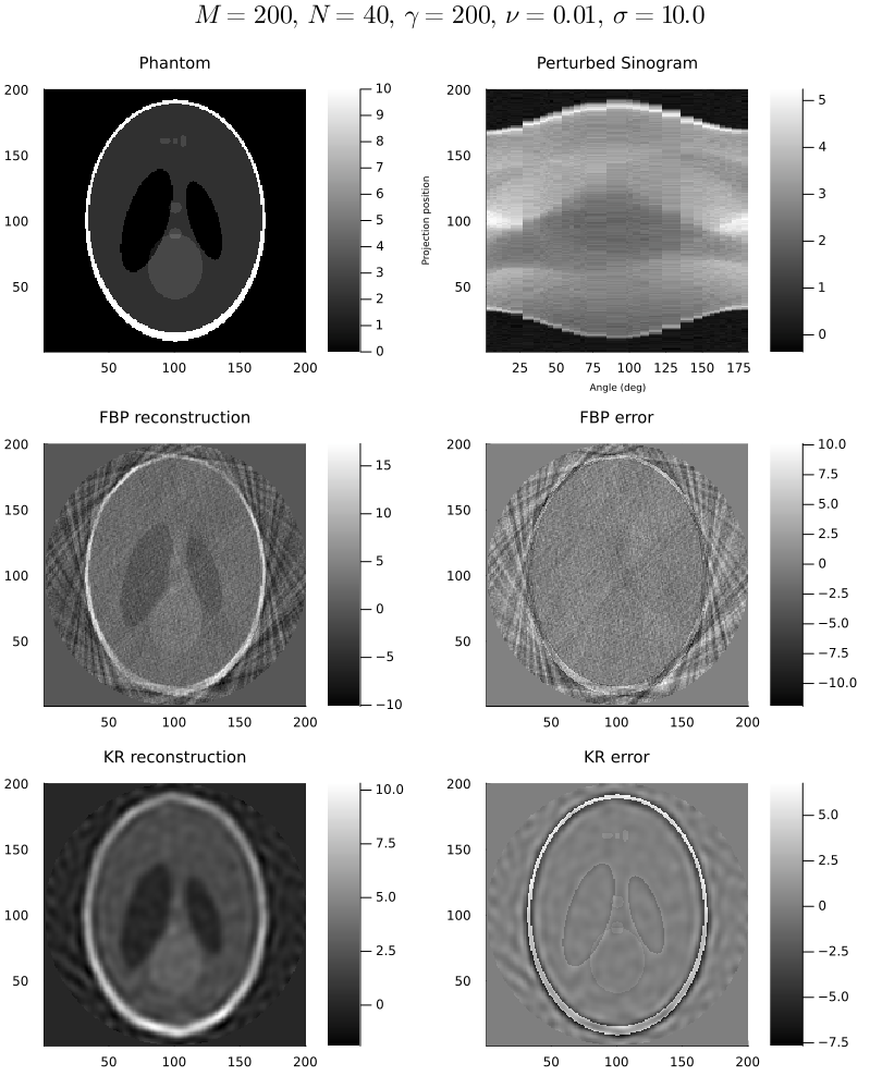
Figure 4: Reconstructions of a noisy sinogram (top right) at $N=40$ randomly chosen angles over $[-\pi/2,\pi/2)$ (rad), generated by the $M\times M$ ($M=200$) pixelated 2D Shepp-Logan phantom (top left). The noise level $\sigma=10$ is added to the sinogram.

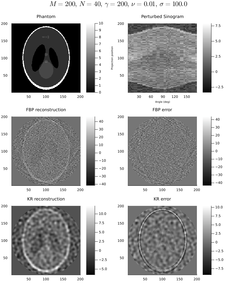
Figure 5: Reconstructions of a noisy sinogram (top right) at $N=40$ randomly chosen angles over $[-\pi/2,\pi/2)$ (rad), generated by the $M\times M$ ($M=200$) pixelated 2D Shepp-Logan phantom (top left). The noise level $\sigma=100$ is added to the sinogram.

The two algorithms exhibit an important difference with regards to dimension. The FBP algorithm’s approach varies between even and odd dimensions: filtering is a local operation for $n=3$, whereas filtering for $n=2$, the Hilbert transform, involves convolution with a nowhere-zero function, necessitating global information for reconstruction [20]. In contrast, our methodology remains consistent across different dimensions $n$.

Though our methodology is dimension-agnostic, specific integral geometries can be leveraged to ease the computational burden associated with solving the normal equation (14). We demonstrate in Section 5 that when $n=2$, a parallel geometry only requires $O(NM^{2}+NM\log N)$ operations, i.e. the same amount of computation as FBP implemented with the aid of the FFT.

4 Invariant Kernels

4.1 Rotation Invariant Kernel

We have thus far explored the tomographic reconstruction problem without making any assumptions about the reproducing kernel $K$ on $\mathbb{B}^{n}$. At this level of generality, the induced reproducing kernel for the projection image space will depend on the orientation $R\in SO(n)$: for any $\mathbf{x}_{1},\mathbf{x}_{2}\in\mathbb{B}^{n-1}$,

$$\tilde{K}^{R}(\mathbf{x}_{1},\mathbf{x}_{2})=\int_{I_{\|\mathbf{x}_{2}\|}}\int_{I_{\|\mathbf{x}_{1}\|}}K(R^{\top}[\mathbf{x}_{1}:z_{1}],R^{\top}[\mathbf{x}_{2}:z_{2}])\mathrm{d}z_{1}\mathrm{d}z_{2}.$$ (15)

When practitioners suspect a high degree of asymmetry in the original structure, they might opt to choose a suitable kernel that matches this asymmetry. In such cases, multiple induced kernels are likely useful, each corresponding to a different orientation. However, for most purposes, it would be desirable to use a kernel that ensures the induced kernel (and corresponding RKHS) remains invariant regardless of the choice of orientations. Additionally, when the orientations $R_{1},\dots,R_{N}\in SO(n)$ are unknown as in cryo-EM, the dependence of (15) on $R\in SO(n)$ poses a major obstruction, as it becomes unclear which domain $\mathbb{H}(\tilde{K}^{R})$ should be used for the micrographs. To address this issue, we consider a specific class of kernels known as rotation-invariant kernels.

Definition 4.1.

Let $E$ be a subset of $\mathbb{R}^{n}$ containing $0$, on which the rotation group $SO(n)$ acts from the left. A bivariate function $K:E\times E\rightarrow\mathbb{R}$ is called rotation-invariant if for any $R\in SO(n)$,

$$K(\mathbf{z}_{1},\mathbf{z}_{2})=K(R^{\top}\mathbf{z}_{1},R^{\top}\mathbf{z}_{2}),\quad\mathbf{z}_{1},\mathbf{z}_{2}\in E.$$

When $K:\mathbb{B}^{n}\times\mathbb{B}^{n}\rightarrow\mathbb{R}$ is a rotation-invariant kernel on $\mathbb{B}^{n}$, it is straightforward that the induced kernel $\tilde{K}^{R}=(\mathscr{P}_{R}\times\mathscr{P}_{R})K$ in (15) does not depend on $R\in SO(n)$. Consequently, we will suppress the dependency on $R$ and will denote the induced kernel by $\tilde{K}$, and the induced generator at $\mathbf{x}\in\mathbb{B}^{n-1}$ by $\tilde{k}_{\mathbf{x}}$. Moving forward, we will consistently assume that our chosen kernel $K:\mathbb{B}^{n}\times\mathbb{B}^{n}\rightarrow\mathbb{R}$ is a continuous rotation-invariant kernel. To simplify notation, when there is no potential for ambiguity, we will write the RKHSs $\mathbb{H},\tilde{\mathbb{H}}$ and $\mathbb{H}_{R}$, instead of $\mathbb{H}(K),\mathbb{H}(\tilde{K})$ and $\mathbb{H}_{R}(K)=\mathcal{R}(\mathscr{P}_{R}^{*})$, respectively.

Below, we show that the rotation-invariance on $K:\mathbb{B}^{n}\times\mathbb{B}^{n}\rightarrow\mathbb{R}$ induces the reflection-invariance when $n\geq 3$. Note that the orthogonal group $O(n)=SO(n)\rtimes\{I,J\}$ is the semidirect product of $SO(n)$ and $\{I,J\}$.

Theorem 4.2.

Let $n\geq 3$ and $K:\mathbb{B}^{n}\times\mathbb{B}^{n}\rightarrow\mathbb{R}$ be a rotation-invariant kernel. Then $K$ is invariant under the left action of $O(n)$, i.e. for any $R\in O(n)$,

$$K(\mathbf{z}_{1},\mathbf{z}_{2})=K(R^{\top}\mathbf{z}_{1},R^{\top}\mathbf{z}_{2}),\quad\mathbf{z}_{1},\mathbf{z}_{2}\in\mathbb{B}^{n}.$$

For any $f\in\mathbb{H}$, its reflection $Jf$ defined by $Jf(\mathbf{z}):=f(J\mathbf{z})$ leads to the same projection image at a conjugacy angle $JR^{\top}J\in SO(n)$:

$$\mathscr{P}_{R}Jf(\mathbf{x})=\int_{I_{\|\mathbf{x}\|}}Jf(R^{\top}[\mathbf{x}:z])\mathrm{d}z=\int_{I_{\|\mathbf{x}\|}}f(JR^{\top}J[\mathbf{x}:-z])\mathrm{d}z=\mathscr{P}_{JR^{\top}J}f(\mathbf{x}),$$

This reveals that when the orientations are not known, it is impossible to determine the handedness of the structure. It is often more convenient and mathematically natural to work with $O(n)$-invariance, as $O(n)$ includes all the unitary representations in $\mathbb{R}^{n}$. Nonetheless, Theorem 4.2 implies that $SO(n)$-invariance is sufficient to retrieve $O(n)$-invariance in the case where $n\geq 3$.

Proposition 4.3.

Let $K:\mathbb{B}^{n}\times\mathbb{B}^{n}\rightarrow\mathbb{R}$ be a rotation-invariant kernel. Then $\tilde{K}:\mathbb{B}^{n-1}\times\mathbb{B}^{n-1}\rightarrow\mathbb{R}$ is invariant under the left action of $O(n-1)$.

Drawing an analogy, one might expect that if $K:\mathbb{B}^{n}\times\mathbb{B}^{n}\rightarrow\mathbb{R}$ is translation-invariant, then $\tilde{K}$ would inherit this property. However, this is not true. Although the integration intervals $I_{\|\mathbf{x}_{1}\|},I_{\|\mathbf{x}_{2}\|}$ for $\tilde{K}^{R}$ are independent of rotations, they do rely on the values of $\mathbf{x}_{1}$ and $\mathbf{x}_{2}$ in $\mathbb{B}^{n-1}$. One potential approach to maintain translation invariance might involve extending the domain of $K$ from $\mathbb{B}^{n}$ to $\mathbb{R}^{n}$. Unfortunately, this approach presents a more significant challenge: it results in blowing up $\tilde{K}(\mathbf{x}_{1},\mathbf{x}_{2})$ to infinity as $\int_{-\infty}^{+\infty}K([\mathbf{x}_{1}:z_{1}],[\mathbf{x}_{2}:z_{2}])\mathrm{d}z_{1}$ does not depend on $z_{2}$. Consequently, the hope that the induced kernel $\tilde{K}$ becomes isotropic is abandoned.

Corollary 4.4.

Let $K:\mathbb{B}^{n}\times\mathbb{B}^{n}\rightarrow\mathbb{R}$ be a rotation-invariant kernel. If $R_{1}\sim R_{2}\in SO(n)$ as defined in (1), then the range space of the backprojections $\mathscr{P}_{R_{1}}^{*}$ and $\mathscr{P}_{R_{2}}^{*}$ are the same, i.e. $\mathbb{H}_{R_{1}}=\mathbb{H}_{R_{2}}$.

While the induced RKHS $\tilde{\mathbb{H}}=\mathbb{H}(\tilde{K})$ remains invariant to orientations, Corollary 4.4 highlights that the range space $\mathbb{H}_{R}=\mathcal{R}(\mathscr{P}_{R}^{*})$ of the backprojection depends on the axis of the orientation. Thus, we cannot hope to get an expression for $\mathscr{P}_{R_{i}}^{*}\circ\mathscr{P}_{R_{i^{\prime}}}:\mathbb{H}\rightarrow\mathbb{H}_{R_{i}}$ in terms of the relative angles $R_{i}R_{i^{\prime}}^{\top}$. On the other hand, Theorem 4.7 indicates that $\mathscr{P}_{R_{i}}\circ\mathscr{P}_{R_{i^{\prime}}}^{*}:\tilde{\mathbb{H}}\rightarrow\tilde{\mathbb{H}}$ depends solely on the relative angles, and consequently, so does the Gram matrix $\mathbf{W}$ of the X-ray representer theorem, as well.

4.2 Representation Theory

When $K:\mathbb{B}^{n}\times\mathbb{B}^{n}\rightarrow\mathbb{R}$ is rotation-invariant, the corresponding RKHS $\mathbb{H}=\mathbb{H}(K)$ also inherits the same invariance in that $f\in\mathbb{H}$ if and only if $f(R^{\top}\,\cdot)\in\mathbb{H}$ for any $R\in SO(n)$. This is because

$$k_{\mathbf{z}_{1}}(R^{\top}\mathbf{z}_{2})=K(\mathbf{z}_{1},R^{\top}\mathbf{z}_{2})=K(R\mathbf{z}_{1},\mathbf{z}_{2})=k_{R\mathbf{z}_{1}}(\mathbf{z}_{2}).$$ (16)

for any $\mathbf{z}_{1},\mathbf{z}_{2}\in\mathbb{B}^{n}$ and $R\in SO(n)$. More formally:

Definition 4.5.

For a continuous rotation-invariant kernel $K:\mathbb{B}^{n}\times\mathbb{B}^{n}\rightarrow\mathbb{R}$, define the left-regular representaiton to be a map $\rho:SO(n)\rightarrow\mathcal{B}(\mathbb{H}),R\mapsto\rho(R)$, given by

$$(\rho(R)f)(\mathbf{z}):=f(R^{\top}\mathbf{z}),\quad R\in SO(n),\,\mathbf{z}\in\mathbb{B}^{n},\,f\in\mathbb{H}.$$

In this notation (16) can be re-interpreted as $\rho(R)k_{\mathbf{z}}=k_{R\mathbf{z}}$, illustrating that applying a rotation operator to a function is equivalent to the inverse rotation of the evaluation point. This correspondence between rotating functions and rotating evaluation points highlights that consecutive rotations of a function corresponds to cumulative rotations of the evaluation point. Moreover, the norm of the function remains unaffected during this process, as the kernel is rotation invariant. It is thus not surprising that we can state the following proposition.

Proposition 4.6.

Given a continuous rotation-invariant kernel $K:\mathbb{B}^{n}\times\mathbb{B}^{n}\rightarrow\mathbb{R}$, the left-regular representation $(\rho,\mathbb{H})$ is a unitary representation of $SO(n)$.

As a direct consequence, for any $R\in SO(n)$, we have $\rho(R)^{*}=\rho(R)^{-1}=\rho(R^{\top})$. It follows that for any $f_{1},f_{2}\in\mathbb{H}$, we get $\langle\rho(R)f_{1},f_{2}\rangle_{\mathbb{H}(K)}=\langle f_{1},\rho(R^{\top})f_{2}\rangle_{\mathbb{H}(K)}$, implying that taking an inner product between two functions after rotating one function is equivalent to taking an inner product after rotating the other function in the opposite direction.

The projection image at orientation $R\in SO(n)$ is equivalent to a projection image along the $e_{n}$-axis, after rotating the original object by the left action of $\rho(R)$. We thus arrive at the following theorem, which again highlights the natural analogy between the RKHS X-ray transform and the Euclidean projection - Proposition 2.1.

Theorem 4.7 (Representation).

Let $K:\mathbb{B}^{n}\times\mathbb{B}^{n}\rightarrow\mathbb{R}$ be a continuous rotation-invariant kernel. For any $R,R_{1},R_{2}\in SO(n)$, it holds that

1. The X-ray transform is obtained as $\mathscr{P}_{R}=\mathscr{P}_{I}\circ\rho(R):\mathbb{H}\rightarrow\tilde{\mathbb{H}}$.

2. The Backprojection is obtained as $\mathscr{P}_{R}^{*}=\rho(R^{\top})\circ\mathscr{P}_{I}^{*}:\tilde{\mathbb{H}}\rightarrow\mathbb{H}$.

3. The Back-then-forward projection operation is obtained as $\mathscr{P}_{R_{1}}\circ\mathscr{P}_{R_{2}}^{*}=\mathscr{P}_{I}\circ\rho(R_{1}R_{2}^{\top})\circ\mathscr{P}_{I}^{*}:\tilde{\mathbb{H}}\rightarrow\tilde{\mathbb{H}}$.

Therefore, for any $\mathbf{x}_{j},\mathbf{x}_{k}\in\mathbb{B}^{n-1}$,

$$(\mathscr{P}_{R_{1}}\circ\mathscr{P}_{R_{2}}^{*}\tilde{k}_{\mathbf{x}_{k}})(\mathbf{x}_{j})=\langle(\rho(R_{1}R_{2}^{\top})\circ\mathscr{P}_{I}^{*})\tilde{k}_{\mathbf{x}_{k}},\mathscr{P}_{I}^{*}\tilde{k}_{\mathbf{x}_{j}}\rangle_{\mathbb{H}}.$$

As a direct consequence, we get $\mathbb{H}_{R}^{\perp}=\mathcal{N}(\mathscr{P}_{R})=\rho(R^{\top})\mathcal{N}(\mathscr{P}_{I})=\rho(R^{\top})\mathbb{H}_{I}^{\perp}$. At this point, it is worthwhile to revisit our representer theorem Theorem 3.9, which made no invariance assumption. If we do assume rotation-invariance, we get a better formulation for the corresponding Gram matrix $\mathbf{W}=[w_{ij,i^{\prime}j^{\prime}}]$. Specifically, we can write

$$w_{ij,i^{\prime}j^{\prime}} =\langle\mathscr{P}_{R_{i}}^{*}\tilde{k}_{\mathbf{x}_{j}},\mathscr{P}_{R_{i^{\prime}}}^{*}\tilde{k}_{\mathbf{x}_{j^{\prime}}}\rangle_{\mathbb{H}}=(\mathscr{P}_{R_{i}}\circ\mathscr{P}_{R_{i^{\prime}}}^{*}\tilde{k}_{\mathbf{x}_{j^{\prime}}})(\mathbf{x}_{j})$$ (17)

$$=(\mathscr{P}_{I}\circ\rho(R_{i}R_{i^{\prime}}^{\top})\circ\mathscr{P}_{I}^{*}\tilde{k}_{\mathbf{x}_{j^{\prime}}})(\mathbf{x}_{j})$$

$$=\int_{I_{\|\mathbf{x}_{j^{\prime}}\|}}\int_{I_{\|\mathbf{x}_{j}\|}}K([\mathbf{x}_{j}:z_{1}],R_{i}R_{i^{\prime}}^{\top}[\mathbf{x}_{j^{\prime}}:z_{2}])\mathrm{d}z_{1}\mathrm{d}z_{2}.$$

And, recalling that when $R_{i}=R_{i^{\prime}}$, the back-then-forward projection is the identity map on $\tilde{\mathbb{H}}$, i.e. $\mathscr{P}_{R_{i}}\circ\mathscr{P}_{R_{i}}^{*}=\mathscr{P}_{I}\circ\rho(I)\circ\mathscr{P}_{I}^{*}=I$, we arrive at

$$w_{ij,ij^{\prime}}=\tilde{K}(\mathbf{x}_{j},\mathbf{x}_{j^{\prime}})=\int_{I_{\|\mathbf{x}_{j}\|}}\int_{I_{\|\mathbf{x}_{j}\|}}K([\mathbf{x}_{j}:z_{1}],[\mathbf{x}_{j^{\prime}}:z_{2}])\mathrm{d}z_{1}\mathrm{d}z_{2}.$$

We now move on to the question of explicit decompositions/representations of continuous $O(n)$-invariant kernels and their corresponding RKHS. To this aim, we can make use of classical results concerning spherical harmonics, which can be found in Appendix C. For any $\lambda>-1/2$, the Gegenbauer polynomials $C_{l}^{\lambda}$ of degree $l$ are orthogonal polynomials on $[-1,+1]$ with the weight function $w^{2\lambda-1}$, normalized by $C_{l}^{\lambda}(1)=1$ as in [20]. The RKHS $\mathbb{H}(C_{l}^{n/2-1})$ spans $\mathcal{H}_{l}(\mathbb{S}^{n-1})$ and possesses an ONB $\{(p^{n/2-1}_{l}|\mathbb{S}^{n-2}|)^{1/2}Y_{lk}(\theta):k=1,2,\dots,N(n,l)\}$, see (30) and (29) for the explicit formula of the constant $p^{n/2-1}_{l}=\|C_{l}^{n/2-1}\|^{2}_{\mathcal{L}_{2}(w^{2\lambda-1})}>0$. Using this result, we show that any continuous $O(n)$-invariant kernel $K:\mathbb{B}^{n}\times\mathbb{B}^{n}\rightarrow\mathbb{R}$ can be decomposed as a countable sum of the multiplication of radial kernels $c_{l}$ and Gegenbauer polynomials $C_{l}^{n/2-1}$, thus $K$ is entirely determined by radial kernels.

Theorem 4.8 (Generalized Schoenberg).

The following are equivalent.

1. A continuous kernel $K:\mathbb{B}^{n}\times\mathbb{B}^{n}\rightarrow\mathbb{R}$ is invariant under the left action of $O(n)$.

2. There exists continuous radial kernels $c_{l}:[0,1]\times[0,1]\rightarrow\mathbb{R}$ with $c_{l}(0,0)=0$ for $l\geq 1$ and $\max_{r\in[0,1]}\sum_{l=0}^{\infty}c_{l}(r,r)<\infty$ such that $K=\sum_{l=0}^{\infty}c_{l}\otimes C_{l}^{n/2-1}$, i.e. for any $r_{1},r_{2}\in[0,1]$ and $\theta_{1},\theta_{2}\in\mathbb{S}^{n-1}$,

   $$K(r_{1}\theta_{1},r_{2}\theta_{2})=\sum_{l=0}^{\infty}c_{l}(r_{1},r_{2})C_{l}^{n/2-1}(\theta_{1}^{\top}\theta_{2}),$$ (18)

   where the sum converges absolutely and uniformly.

Also, the $l$-th radial kernel $c_{l}$ is given by

$$c_{l}(r_{1},r_{2})=\frac{1}{p^{n/2-1}_{l}|\mathbb{S}^{n-2}|}\int_{\mathbb{S}^{n-1}}K(r_{1}\theta_{1},r_{2}\theta_{2})C_{l}^{n/2-1}(\theta_{1}^{\top}\theta_{2})\mathrm{d}\theta_{2},$$

independent of the choice of $\theta_{1}\in\mathbb{S}^{n-1}$.

Our next theorem is a generalization of Aronszajn [3, Section 6] and spectrally characterises the RKHS associated with an invariant kernel, where (4.9) might be referred to as a Picard criterion.

Theorem 4.9 (Generalized Mercer).

Let $K:\mathbb{B}^{n}\times\mathbb{B}^{n}\rightarrow\mathbb{R}$ be an $O(n)$-invariant countinuous kernel, associated with continuous radial kernels $c_{l}:[0,1]\times[0,1]\rightarrow\mathbb{R}$ as in Theorem 4.8. Then, the corresponding RKHS and norm are given by

$$\mathbb{H}(K)= \left\{\sum_{l=0}^{\infty}\sum_{k=1}^{N(n,l)}h_{lk}(r)Y_{lk}(\theta):h_{lk}\in\mathbb{H}(c_{l}),\sum_{l=0}^{\infty}\sum_{k=1}^{N(n,l)}\frac{\|h_{lk}\|^{2}_{\mathbb{H}(c_{l})}}{p^{n/2-1}_{l}|\mathbb{S}^{n-2}|}<\infty\right\},$$

$$\left\|\sum_{l=0}^{\infty}\sum_{k=1}^{N(n,l)}h_{lk}Y_{lk}\right\|^{2}_{\mathbb{H}(K)}=\sum_{l=0}^{\infty}\sum_{k=1}^{N(n,l)}\frac{\|h_{lk}\|^{2}_{\mathbb{H}(c_{l})}}{p^{n/2-1}_{l}|\mathbb{S}^{n-2}|}<\infty,$$ (19)

where $\left\{Y_{lk}(\theta):k=1,2,\dots,N(n,l)\right\}$ is an orthonormal basis (ONB) of $\mathcal{H}_{l}(\mathbb{S}^{n-1})$ with respect to the $\mathcal{L}_{2}$ norm.

Remark 4.10.

Consider a simple case in Theorem 4.9 where $K=c\otimes C_{l}^{n/2-1}$ for some $l\in\mathbb{N}$. We further assume that the radial kernel satisfies $c(r_{1},r_{2})=e(r_{1})e(r_{2})$ for some continuous function $e:[0,1]\rightarrow\mathbb{R}$, so that $\mathbb{H}(c)$ is simply the one-dimensional space spanned by $e$ with $\|e\|_{\mathbb{H}(c)}=1$ by Proposition 2.19 in [22]. In this case, $\mathbb{H}(K)=\text{span}\left\{e(r)Y_{lk}(\theta):k=1,2,\dots,N(n,l)\right\}$ is an $N(n,l)$-dimensional space with an ONB

$$\left\{(p^{n/2-1}_{l}|\mathbb{S}^{n-2}|)^{1/2}e(r)Y_{lk}(\theta):k=1,2,\dots,N(n,l)\right\}.$$ (20)

To describe the unitary representation $\rho(R)$ of $\mathbb{H}(K)$, recall that the Wigner D-matrix $D_{l}(R)$ of degree $l$ in (27) is the irreducible unitary representation of $\mathcal{H}_{l}(\mathbb{S}^{n-1})$. Therefore, if we identify $\mathbb{H}(K)$ as an inner product space with respect to the ONB in (20), then the unitary representation $\rho(R)$ reduces to $D_{l}(R)$.

The remark above sheds light on how truncated singular value decomposition [12, 37] can be incorporated into our RKHS framework. When viewing the X-ray transform as an integral operator $\mathscr{P}_{R}:\mathcal{L}_{2}(\mathbb{B}^{n})\rightarrow\mathcal{L}_{2}(SO(n)\times\mathbb{B}^{n-1},W^{-1/2})$, its singular functions with non-zero singular values become $\{Z_{ml}(r)Y_{lk}(\theta):m\in\mathbb{N}_{0},0\leq l\leq m,1\leq k\leq N(n,l),2|(m-l)\}$, where $Z_{ml}$ is the Zernike radial polynomial, and $\{Y_{lk}(\theta):k=1,\dots,N(n,l)\}$ is a carefully chosen ONB for $\mathcal{H}_{l}(\mathbb{S}^{n-1})$ [18, 14]. Truncating with respect to the $m$ index at level $T\in\mathbb{N}$ and applying the pseudo-inverse of $\mathscr{P}_{R}$ for reconstruction, it is effectively the same as working within our RKHS framework with the kernel

$$K(r_{1}\theta_{1},r_{2}\theta_{2})=\sum_{m=0}^{T}\sum_{\begin{subarray}{c}l\leq m\\ 2|(m-l)\end{subarray}}Z_{ml}(r_{1})Z_{ml}(r_{2})C_{l}^{n/2-1}(\theta_{1}^{\top}\theta_{2}),$$

and the matrix notation of the unitary representation $\rho(R)$ of $\mathbb{H}(K)$ becomes

$$[\rho(R)]_{mlk,m^{\prime}l^{\prime}k^{\prime}}=\delta_{ll^{\prime}}\cdot[D_{l}(R)]_{kk^{\prime}},$$

where $\delta_{ll^{\prime}}$ is the Kronecker delta. Note that this kernel is not strictly p.d. as it spans a finite-dimensional space, as opposed to the Gaussian kernel. Similarly, if we wish to interpret the RKHS norm as a measure of smoothness, we can derive a kernel in terms of Fourier-Bessel functions, which are the eigenfunctions of the Laplacian in the unit disk with vanishing Dirichlet boundary conditions [37, 36].

The preceding argument illustrates why our RKHS approach is less likely to produce artifacts. In situations where viewing angles are limited, truncated SVD imposes restrictions on the angular frequency, adhering to the Nyquist-Shannon sampling theorem. The spherical average of any spherical harmonic with a positive degree is always zero, and consequently, the spherical average of the original structure can only be influenced by the first spherical harmonic $Y_{0}$, which is a constant function. This can result in generating negative signals in the reconstruction image, even when the true image only contains positive values, leading to a symmetric reconstruction error, as vividly demonstrated in Section 3.5. Even if one performs the sinogram interpolation to reduce the magnitude of error, they remain constrained by the limits of resolution, due to the discussion following Theorem 2.9.

In contrast, Theorem 4.8 reveals that the RKHS approach can adeptly combine a countably infinite multitude of band-limited kernels, such as Gaussian kernels. Also, the reconstruction does not rely on the Fourier transform but instead employs linear regression. Additionally, the level of desired smoothness can be finely controlled via the Picard condition (4.9). Consequently, our approach appears to avoid generating negative signals while minimizing the squared loss based on the provided sinogram.

5 Circulant Algorithm

We now show that, in the case of a parallel geometry in the plane, one can employ a rotation-invariant kernel, and implement an RKHS-based reconstruction efficiently. Let $n=2$ and assume that the projection angles are equiangular. Using the isomorphic relationships

$$\phi\in\mathbb{R}/2\pi\mathbb{Z}\ \cong\ \theta(\phi)=\begin{pmatrix}\sin\phi\\ \cos\phi\end{pmatrix}\in\mathbb{S}^{1}\ \cong\ E(\phi)=\begin{pmatrix}\cos\phi&-\sin\phi\\ \sin\phi&\cos\phi\end{pmatrix}\in SO(2),$$ (21)

we identify $R_{i}=E(\phi_{i})\in SO(2)$ with $\phi_{i}=i\cdot 2\pi/N$ for $i=1,\dots,N$, and the relative angles are given by $R_{i}R_{i^{\prime}}^{\top}=E(\phi_{i}-\phi_{i^{\prime}})$. The Gram matrix $\mathbf{W}\in\mathbb{R}^{NM\times NM}$ is a $N\times N$ block Toeplitz matrix of $M\times M$ matrices $\mathbf{W}_{ii^{\prime}}$, whose $j,j^{\prime}$ element is given by (17):

$$\left[\mathbf{W}_{ii^{\prime}}\right]_{jj^{\prime}}:=w_{ij,i^{\prime}j^{\prime}}=\langle\mathscr{P}_{\phi_{i}}^{*}\tilde{k}_{\mathbf{x}_{j}},\mathscr{P}_{\phi_{i^{\prime}}}^{*}\tilde{k}_{x_{j^{\prime}}}\rangle_{\mathbb{H}(K)}=(\mathscr{P}_{(\phi_{i}-\phi_{i^{\prime}})}\circ\mathscr{P}_{0}^{*}\tilde{k}_{x_{j^{\prime}}})(x_{j}).$$

As $\mathbf{W}_{ii^{\prime}}$ only depends on $(i-i^{\prime})(\text{mod }N)$, we denote each block $\mathbf{W}_{ii^{\prime}}$ by $\mathbf{W}_{(i-i^{\prime})}$ so that the Gram matrix becomes a block circulant matrix $\mathbf{W}=[\mathbf{W}_{ii^{\prime}}]=[\mathbf{W}_{(i-i^{\prime})}]$ with $\mathbf{W}_{-i}=\mathbf{W}_{N-i}=\mathbf{W}_{i}^{\top}$. The normal equation in (14) in terms of the block matrix is given by

$$\begin{pmatrix}\mathbf{W}_{0}+\gamma I&\mathbf{W}_{N-1}&\dots&\mathbf{W}_{1}\\ \mathbf{W}_{1}&\mathbf{W}_{0}+\gamma I&\dots&\mathbf{W}_{2}\\ \vdots&\vdots&\ddots&\vdots\\ \mathbf{W}_{N-1}&\mathbf{W}_{N-2}&\dots&\mathbf{W}_{0}+\gamma I\end{pmatrix}\begin{pmatrix}\boldsymbol{\alpha}_{1}\\ \boldsymbol{\alpha}_{2}\\ \vdots\\ \boldsymbol{\alpha}_{N-1}\end{pmatrix}=\begin{pmatrix}\mathbf{Y}_{1}\\ \mathbf{Y}_{2}\\ \vdots\\ \mathbf{Y}_{N-1}\end{pmatrix}.$$

For $i=1,\dots,N$, $\mathbf{Y}_{i}=\sum_{k=0}^{N-1}\mathbf{W}_{i-k}\boldsymbol{\alpha}_{k}+\gamma\boldsymbol{\alpha}_{i}$, and its discrete ($M$-dimensional) Fourier transform becomes

$$\widehat{\mathbf{Y}}_{i}: =\frac{1}{N}\sum_{l=0}^{N-1}e^{-2\pi\imath il/N}\mathbf{Y}_{l}$$

$$=\frac{1}{N}\sum_{l=0}^{N-1}\sum_{k=0}^{N-1}e^{-2\pi\imath il/N}\mathbf{W}_{l-k}\boldsymbol{\alpha}_{k}+\frac{\gamma}{N}\sum_{l=0}^{N-1}e^{-2\pi\imath il/N}\boldsymbol{\alpha}_{l}$$

$$=\frac{1}{N}\sum_{k=0}^{N-1}e^{-2\pi\imath ik/N}\boldsymbol{\alpha}_{k}\left(\sum_{l=0}^{N-1}e^{-2\pi\imath i(l-k)/N}\mathbf{W}_{l-k}\right)+\frac{\gamma}{N}\sum_{l=0}^{N-1}e^{-2\pi\imath il/N}\boldsymbol{\alpha}_{l}$$

$$=\left(\sum_{l=0}^{N-1}e^{-2\pi\imath il/N}\mathbf{W}_{l}+\gamma I\right)\left(\frac{1}{N}\sum_{k=0}^{N-1}e^{-2\pi\imath ik/N}\boldsymbol{\alpha}_{k}\right)$$

$$=N\left(\frac{1}{N}\sum_{l=0}^{N-1}e^{-2\pi\imath il/N}\mathbf{W}_{l}+\frac{\gamma}{N}I\right)\widehat{\boldsymbol{\alpha}}_{i}=N\left(\widehat{\mathbf{W}}_{i}+\frac{\gamma}{N}I\right)\widehat{\boldsymbol{\alpha}}_{i}.$$

Hence, we obtain the following algorithm.

Algorithm 1 Kernel Reconstruction with Parallel Geometry

$\mathbf{Y}\in\mathbb{R}^{N\times M}$

$\boldsymbol{\alpha}\in\mathbb{R}^{N\times M}$

procedure KR($Y$)$\triangleright$ Solution of the normal equation

     for $i\leftarrow 1$ to $N$ do

         for $j,j^{\prime}\leftarrow 1$ to $M$ do

              $[\mathbf{W}_{i}]_{jj^{\prime}}\leftarrow(\mathscr{P}_{\phi_{i}}\circ\mathscr{P}_{0}^{*}\tilde{k}_{x_{j^{\prime}}})(x_{j})$               

     FFT for $\widehat{\mathbf{W}}_{i}\leftarrow\frac{1}{N}\sum_{l=0}^{N-1}e^{-2\pi\imath il/N}\mathbf{W}_{l}$

     FFT for $\widehat{\mathbf{Y}}_{i}\leftarrow\frac{1}{N}\sum_{l=0}^{N-1}e^{-2\pi\imath il/N}\mathbf{Y}_{l}$$\triangleright$ $O(NM\log N)$

     for $i\leftarrow 1$ to $N$ do

         $\widehat{\boldsymbol{\alpha}}_{i}\leftarrow\frac{1}{N}\left(\widehat{\mathbf{W}}_{i}+\frac{\gamma}{N}I\right)^{-1}\widehat{\mathbf{Y}}_{i}$$\triangleright$ $O(NM^{2})$      

     Inverse FFT for $\boldsymbol{\alpha}_{i}\leftarrow\sum_{l=0}^{N-1}e^{2\pi\imath il/N}\widehat{\boldsymbol{\alpha}}_{l}$$\triangleright$ $O(NM\log N)$

     return $\boldsymbol{\alpha}$

If the kernel and the grid are pre-determined so that regularized block inverse matrices $(\widehat{\mathbf{W}}_{i}+\gamma I/N)^{-1}$ are stored, then the algorithm described above can be efficiently solved using fast Fourier transform (FFT) with a computational complexity of $O(NM^{2}+NM\log N)$. This computational complexity is equivalent to that of the discretized FBP algorithm. Moreover, this approach not only offers computational efficiency but also enhances stability by performing inversions of $M\times M$ matrices instead of dealing with the Gram matrix of size $NM\times NM$.

6 Concluding Remarks

While our primary focus has been on the X-ray transform, our RKHS framework can be readily extended to the $k$-plane transform [5]. For $1\leq k\leq n$, the $k$-plane transform $\mathscr{K}_{R}:\mathcal{L}_{2}(\mathbb{B}^{n})\rightarrow\mathcal{L}_{2}(\mathbb{B}^{n-k})$ at orientation $R\in SO(n)$ is given by

$$\mathscr{K}_{R}f(\mathbf{x})=\int_{W(\mathbf{x})\cdot\mathbb{B}^{k}}f(R^{\top}[\mathbf{x}:z])\mathrm{d}z,\quad\mathbf{x}\in\mathbb{B}^{n-k}.$$

Define an induced kernel $\tilde{K}^{R}:\mathbb{B}^{n-k}\times\mathbb{B}^{n-k}\rightarrow\mathbb{R}$ as follows:

$$\tilde{K}^{R}(\mathbf{x}_{1},\mathbf{x}_{2}):=\int_{W(\mathbf{x}_{2})\cdot\mathbb{B}^{k}}\int_{W(\mathbf{x}_{1})\cdot\mathbb{B}^{k}}K(R^{\top}[\mathbf{x}_{1}:z_{1}],R^{\top}[\mathbf{x}_{2}:z_{2}])\mathrm{d}z_{1}\mathrm{d}z_{2}.$$

With this extension, our fundamental theorem Theorem 3.4 can be easily generalized to the $k$-plane transform $\mathscr{K}_{R}$ using a similar proof mechanism. Consequently, a unified treatment of both the Radon transform ($k=n-1$) and the X-ray transform ($k=1$) is possible.

Theorem 6.1.

For any $R\in SO(n)$, $\mathscr{K}_{R}:\mathbb{H}(K)\rightarrow\mathbb{H}(\tilde{K}^{R})$ is a contractive, surjective, linear map. Its adjoint operator $\mathscr{K}_{R}^{*}:\mathbb{H}(\tilde{K}^{R})\rightarrow\mathbb{H}(K)$ is an isometry, uniquely determined by $\mathscr{K}_{R}^{*}(\tilde{k}^{R}_{\mathbf{x}})=\int_{W(\mathbf{x})\cdot\mathbb{B}^{k}}k_{R^{\top}[\mathbf{x}:z]}\mathrm{d}z,\quad\mathbf{x}\in\mathbb{B}^{n-1}$ in the sense of Bochner integration. Let $\mathbb{H}_{R}(K):=\mathcal{R}(\mathscr{K}_{R}^{*})$ be the range space of the $k$-plane backprojection. Then,

1. $\mathscr{K}_{R}\circ\mathscr{K}_{R}^{*}:\mathbb{H}(\tilde{K}^{R})\rightarrow\mathbb{H}(\tilde{K}^{R})$ is the identity.

2. $\mathbb{H}_{R}(K)=(\mathcal{N}(\mathscr{K}_{R}))^{\perp},(\mathbb{H}_{R}(K))^{\perp}=\mathcal{N}(\mathscr{K}_{R})$.

3. Any $f\in\mathbb{H}(K)$ can be uniquely expressed as a direct sum:

   $$f=(\mathscr{K}_{R}^{*}\circ\mathscr{K}_{R})f\oplus(f-(\mathscr{K}_{R}^{*}\circ\mathscr{K}_{R})f)\in\mathbb{H}_{R}(K)\oplus\mathcal{N}(\mathscr{K}_{R}),$$

   thus $f\in\mathbb{H}_{R}(K)$ if and only if $f=(\mathscr{K}_{R}^{*}\circ\mathscr{K}_{R})f$.

4. For $g\in\mathbb{H}(\tilde{K}^{R})$, we have

   $$\left\{f\in\mathbb{H}(K):g=\mathscr{K}_{R}f\right\}=\mathscr{K}_{R}^{*}g\oplus\mathcal{N}(\mathscr{K}_{R}),$$

   $$\|g\|_{\mathbb{H}(\tilde{K}^{R})}=\|\mathscr{K}_{R}^{*}g\|_{\mathbb{H}(K)}=\min\left\{\|f\|_{\mathbb{H}(K)}:g=\mathscr{K}_{R}f\right\}.$$

Appendix A Gaussian Kernel Reconstruction

As discussed in Section 3.5, the computation of the Gram matrix $\mathbf{W}=\left[w_{ij,i^{\prime}j^{\prime}}\right]\in\mathbb{R}^{NM\times NM}$ can be demanding due to the necessity of performing the double integration in (11) $O(N^{2}M^{2})$ times. However, when employing the Gaussian kernel, arguably the most frequently used isotropic kernel, this computational burden can be significantly mitigated due to the availability of an explicit formula. The (truncated) Gaussian kernel with a tuning parameter $\gamma>0$ is defined by

$$K(\mathbf{z}_{1},\mathbf{z}_{2}):=\exp(-\gamma\|\mathbf{z}_{1}-\mathbf{z}_{2}\|^{2}),\quad\mathbf{z}_{1},\mathbf{z}_{2}\in\mathbb{B}^{n}.$$

The error function on $\mathbb{R}$ is defined by

$$\text{erf}(z):=\frac{2}{\sqrt{\pi}}\int_{0}^{z}e^{-t^{2}}\mathrm{d}t,\quad z\in\mathbb{R}.$$

By the integral by parts, one can easily check that

$$\Phi(z):=\sqrt{\pi}\int_{0}^{z}\text{erf}(t)\mathrm{d}t=\sqrt{\pi}z\cdot\text{erf}(z)+e^{-z^{2}}-1.$$

Proposition A.1.

Let $K:\mathbb{B}^{n}\times\mathbb{B}^{n}\rightarrow\mathbb{R}$ be the Gaussian kernel with $\gamma>0$.

1. For $\mathbf{x}_{1},\mathbf{x}_{2}\in\mathbb{B}^{n-1}$, the induced kernel $\tilde{K}:\mathbb{B}^{n-1}\times\mathbb{B}^{n-1}\rightarrow\mathbb{R}$ is given by

   $$\tilde{K}(\mathbf{x}_{1},\mathbf{x}_{2})=\frac{e^{-\gamma\|\mathbf{x}_{1}-\mathbf{x}_{2}\|^{2}}}{2\gamma}\sum_{i,j\in\mathbb{Z}_{2}}(-1)^{i+j}\Phi[\sqrt{\gamma}((-1)^{i}W(\mathbf{x}_{1})+(-1)^{j}W(\mathbf{x}_{2}))].$$

2. For $\mathbf{x}\in\mathbb{B}^{n-1},\mathbf{z}\in\mathbb{B}^{n}$ and $R\in SO(n)$, the backprojection of the induced generator is given by

   $$\mathscr{P}_{R}^{*}(\tilde{k}_{\mathbf{x}})(\mathbf{z})=\frac{\sqrt{\pi}e^{-\gamma\|\mathbf{x}-\mathbf{P}_{R}(\mathbf{z})\|^{2}}}{2\sqrt{\gamma}}\sum_{i\in\mathbb{Z}_{2}}(-1)^{i}\text{erf}[\sqrt{\gamma}((-1)^{i}W(\mathbf{x})-\mathbf{P}_{R}(\mathbf{z}))].$$

Lemma A.2.

Let $\mathbf{x}_{1},\mathbf{x}_{2}\in\mathbb{B}^{n-1}$, and $R\in SO(n)$. Also, let $(\tilde{R},\mathbf{r})\in SO(n-1)\times\mathbb{S}^{n-1}$ be the Euler decomposition of $R\in SO(n)$ as in Proposition B.1, and $(\tilde{\mathbf{r}},\arccos(r))\in\mathbb{S}^{n-2}\times[0,\pi]$ be the spherical decomposition of $\mathbf{r}\in\mathbb{S}^{n-1}$ as in (22), where $r=e_{n}^{\top}Re_{n}$. Denote by

$$[\tilde{\mathbf{x}}_{2R}:x_{2R}]:=\tilde{R}^{\top}\mathbf{x}_{2},\quad \tilde{\mathbf{x}}_{2R}\in\mathbb{B}^{n-2},\,x_{2R}=e_{n-1}^{\top}\tilde{R}^{\top}\mathbf{x}_{2}\in[-1,+1],$$

$$[\tilde{\mathbf{x}}_{1\mathbf{r}}:x_{1\mathbf{r}}]:=E(\tilde{\mathbf{r}})\mathbf{x}_{1},\quad \tilde{\mathbf{x}}_{1\mathbf{r}}\in\mathbb{B}^{n-2},\,x_{1\mathbf{r}}=\tilde{\mathbf{r}}^{\top}\mathbf{x}_{1}\in[-1,+1],$$

$$\mu_{1}^{R}:=r\cdot x_{1\mathbf{r}}-x_{2R},\quad \mu_{2}^{R}:=x_{1\mathbf{r}}-r\cdot x_{2R}.$$

1. If $R\sim I$, i.e. $|r|=1$, then $\mathbf{x}_{1}=E(\tilde{\mathbf{r}})\mathbf{x}_{1}$ and

   $$\|[\mathbf{x}_{1}:z_{1}]-R^{\top}[\mathbf{x}_{2}:z_{2}]\|^{2}=\|[\tilde{\mathbf{x}}_{1\mathbf{r}}:rx_{1\mathbf{r}}]-\tilde{R}^{\top}\mathbf{x}_{2}\|^{2}+(z_{1}-rz_{2})^{2}.$$

2. If $R\nsim I$, i.e. $|r|<1$, then

   $$\|[\mathbf{x}_{1}:z_{1}]-R^{\top}[\mathbf{x}_{2}:z_{2}]\|^{2}$$

   $$= \|\tilde{\mathbf{x}}_{1\mathbf{r}}-\tilde{\mathbf{x}}_{2R}\|^{2}+\left[\begin{pmatrix}z_{1}\\ z_{2}\end{pmatrix}-\frac{1}{w(r)}\begin{pmatrix}\mu_{1}^{R}\\ \mu_{2}^{R}\end{pmatrix}\right]^{\top}\begin{pmatrix}1&-r\\ -r&1\end{pmatrix}\left[\begin{pmatrix}z_{1}\\ z_{2}\end{pmatrix}-\frac{1}{w(r)}\begin{pmatrix}\mu_{1}^{R}\\ \mu_{2}^{R}\end{pmatrix}\right].$$

The following proposition shows that the Gram matrix $\mathbf{W}$ in (17) can be computed via the cumulative distribution function (CDF) of the standard bivariate normal distribution, regardless of the dimension $n\in\mathbb{N}$. It also demonstrates that the relative angles between the axes of rotations $R_{1},R_{2}\in SO(n)$, which is $r=\mathbf{r}_{1}^{\top}\mathbf{r}_{2}$, could be interepreted as the correlation.

Proposition A.3.

Let $K:\mathbb{B}^{n}\times\mathbb{B}^{n}\rightarrow\mathbb{R}$ be the Gaussian kernel with $\gamma>0$, and let $R_{1},R_{2}\in SO(n)$ be orientations with the relative angle $R=R_{1}R_{2}^{\top}$. Using the same notation to Lemma A.2, the back-then-forward projection of the induced generator is given as follows:

1. If $R_{1}\sim R_{2}$, then

   $$(\mathscr{P}_{R_{1}}\circ\mathscr{P}_{R_{2}}^{*}\tilde{k}_{\mathbf{x}_{2}})(\mathbf{x}_{1})=(\mathscr{P}_{R}\circ\mathscr{P}_{I}^{*}\tilde{k}_{\mathbf{x}_{2}})(\mathbf{x}_{1})=\frac{\exp(-\gamma\|[\tilde{\mathbf{x}}_{1\mathbf{r}}:rx_{1\mathbf{r}}]-\tilde{R}^{\top}\mathbf{x}_{2}\|^{2})}{2\gamma}\times$$

   $$\quad\sum_{i,j\in\mathbb{Z}_{2}}(-1)^{i+j}\Phi[\sqrt{\gamma}((-1)^{i}W(\mathbf{x}_{1})+(-1)^{j}W(\mathbf{x}_{2}))].$$

2. If $R_{1}\nsim R_{2}$, then

   $$(\mathscr{P}_{R}\circ\mathscr{P}_{I}^{*}\tilde{k}_{\mathbf{x}_{2}})(\mathbf{x}_{1})=(\mathscr{P}_{R}\circ\mathscr{P}_{I}^{*}\tilde{k}_{\mathbf{x}_{2}})(\mathbf{x}_{1})=\frac{\pi\cdot\exp(-\gamma\|\tilde{\mathbf{x}}_{1\mathbf{r}}-\tilde{\mathbf{x}}_{2R}\|^{2})}{\gamma w(r)}\times$$

   $$\quad\sum_{i,j\in\mathbb{Z}_{2}}(-1)^{i+j}\Phi_{2}^{r}\left[\sqrt{2\gamma}((-1)^{i}w(r)W(\mathbf{x}_{1})-\mu_{1}^{R}),\sqrt{2\gamma}((-1)^{j}w(r)W(\mathbf{x}_{2})-\mu_{2}^{R})\right],$$

   where $\Phi_{2}^{\rho}(a,b)$ is the CDF of the standardized bivariate normal distribution $(Z_{1},Z_{2})$ with correlation $\rho\in(-1,+1)$, i.e. $\Phi_{2}^{\rho}(a,b)=\mathbb{P}(Z_{1}\leq a,Z_{2}\leq b)$.

In the case where $|r|<1$, we could approximate the bivariate normal integral $\Phi_{2}^{r}$ in terms of the error function for fast computations, see [32]. Moreover, in the case where $n=2$, we get a simpler expression for Propositions A.1 and A.3. Using an isomorphism (21), we identify $R_{1},\dots,R_{N}\in SO(2)$ with $\phi_{1},\dots,\phi_{N}\in\mathbb{R}/2\pi\mathbb{Z}$, i.e. $R_{i}=E(\phi_{i})$ for $i=1,\dots,N$. Note that the relative angles are given by $R_{i}R_{i^{\prime}}^{\top}=E(\phi_{i}-\phi_{i^{\prime}})$.

Corollary A.4.

Let $\mathbf{z}=[z_{1}:z_{2}]\in\mathbb{B}^{2}$, $x_{1},\dots,x_{M}\in\mathbb{B}^{1}=[-1,+1]$, and $\phi_{1},\dots,\phi_{N}\in\mathbb{R}/2\pi\mathbb{Z}$. Also, let $K:\mathbb{B}^{n}\times\mathbb{B}^{n}\rightarrow\mathbb{R}$ be the Gaussian kernel with $\gamma>0$. The backprojection of the induced generator is given by

$$\mathscr{P}_{\phi_{i}}^{*}(\tilde{k}_{x_{j}})(\mathbf{z})=\frac{e^{-\gamma\|x_{j}-\tilde{z}_{\phi_{i}}\|^{2}}\sqrt{\pi}}{2\sqrt{\gamma}}\left[\text{erf}(\sqrt{\gamma}(w(x_{j})-z_{\phi_{i}}))-\text{erf}(\sqrt{\gamma}(-w(x_{j})-z_{\phi_{i}}))\right],$$

where $\tilde{z}_{\phi_{i}}+\imath z_{\phi_{i}}=e^{\imath\phi_{i}}(z_{1}+\imath z_{2})$. The element of the Gram matrix $\mathbf{W}$ in (17) is given as follows: Denoting by $s_{ii^{\prime}}=\sin(\phi_{i}-\phi_{i^{\prime}})$ and $c_{ii^{\prime}}=\cos(\phi_{i}-\phi_{i^{\prime}})$, it holds that

1. If $s_{ii^{\prime}}=0$, then

   $$(\mathscr{P}_{\phi_{i}}\circ\mathscr{P}_{\phi_{i^{\prime}}}^{*}\tilde{k}_{x_{j^{\prime}}})(x_{j})=\tilde{K}(c_{ii^{\prime}}\cdot x_{j},x_{j^{\prime}})$$

   $$=\frac{\exp(-\gamma(c_{ii^{\prime}}\cdot x_{j}-x_{j^{\prime}})^{2})}{2\gamma}\sum_{k,l\in\mathbb{Z}_{2}}(-1)^{k+l}\Phi[\sqrt{\gamma}((-1)^{k}w(x_{j})+(-1)^{l}w(x_{j^{\prime}}))].$$

2. If $s_{ii^{\prime}}\neq 0$, then

   $$(\mathscr{P}_{\phi_{i}}\circ\mathscr{P}_{\phi_{i^{\prime}}}^{*}\tilde{k}_{x_{2}})(x_{1})=\frac{\pi}{\gamma|s_{ii^{\prime}}|}\times$$

   $$\quad\sum_{k,l\in\mathbb{Z}_{2}}(-1)^{k+l}\Phi_{2}^{c_{ii^{\prime}}}\left[\sqrt{2\gamma}((-1)^{k}s_{ii^{\prime}}w(x_{j})-\mu_{1}^{ii^{\prime}}),\sqrt{2\gamma}((-1)^{l}s_{ii^{\prime}}w(x_{j^{\prime}})-\mu_{2}^{ii^{\prime}})\right],$$

   where

   $$\begin{pmatrix}\mu_{1}^{ii^{\prime}}\\ \mu_{2}^{ii^{\prime}}\end{pmatrix}=\begin{pmatrix}c_{ii^{\prime}}&-1\\ 1&-c_{ii^{\prime}}\end{pmatrix}\begin{pmatrix}x_{j}\\ x_{j^{\prime}}\end{pmatrix}=\begin{pmatrix}c_{ii^{\prime}}\cdot x_{j}-x_{j^{\prime}}\\ x_{j}-c_{ii^{\prime}}\cdot x_{j^{\prime}}\end{pmatrix},$$

   and $\Phi_{2}^{\rho}(a,b)$ is defined as in Proposition A.3.

Appendix B Special Orthogonal Group

In Section 4.1, we extensively utilize the special orthogonal group, which we introduce briefly. For more comprehensive details, please refer to [6]. The special orthogonal group, also called the rotation group, is defined by $SO(n)=\{R\in\mathbb{R}^{n\times n}:RR^{\top}=R^{\top}R=I,\det R=1\}$. It consists of all orthogonal matrices of determinant 1 and is a Lie group of dimension $n(n-1)/2$.

For $n\geq 2$, let $\theta\in\mathbb{S}^{n-1}$ have the spherical coordinates $\phi_{1}\in[-\pi,\pi)$ and $\phi_{2},\dots,\phi_{n-1}\in[0,\pi]$, i.e.

$$\theta=\begin{pmatrix}\sin\phi_{n-1}\dots\sin\phi_{3}\sin\phi_{2}\sin\phi_{1}\\ \sin\phi_{n-1}\dots\sin\phi_{3}\sin\phi_{2}\cos\phi_{1}\\ \sin\phi_{n-1}\dots\sin\phi_{3}\cos\phi_{2}\\ \vdots\\ \sin\phi_{n-1}\cos\phi_{n-2}\\ \cos\phi_{n-1}\end{pmatrix}.$$

If $\tilde{\theta}\in\mathbb{S}^{n-2}$ has the spherical coordinates $\phi_{1}\in[-\pi,\pi)$ and $\phi_{2},\dots,\phi_{n-2}\in[0,\pi]$, then the spherical decomposition reads

$$\theta=[\sin\phi_{n-1}\tilde{\theta}:\cos\phi_{n-1}].$$ (22)

For $l=n-1,\dots,1$, let $R^{l}_{\phi}$ be the rotation in $x_{l}$-$x_{l+1}$ plane with angle $\phi$, i.e.

$$R^{l}_{\phi}:=\begin{pmatrix}\mathbf{I}_{l-1}&\vline&\mathbf{0}&\vline&\mathbf{0}\\ \hline\cr\mathbf{0}&\vline&\begin{matrix}\cos\phi&\sin\phi\\ -\sin\phi&\cos\phi\end{matrix}&\vline&\mathbf{0}\\ \hline\cr\mathbf{0}&\vline&\mathbf{0}&\vline&\mathbf{I}_{n-l-1}\end{pmatrix}\in SO(n).$$

The Euler rotation matrix for $\theta\in\mathbb{S}^{n-1}$ is defined by

$$E(\theta)=E(\phi_{1},\dots,\phi_{n-1}):=R^{n-1}_{-\phi_{n-1}}\dots R^{2}_{-\phi_{2}}R^{1}_{-\phi_{1}}\in SO(n).$$

Note that

$$E(\theta)^{\top} =R^{1}_{\phi_{1}}R^{2}_{\phi_{2}}\dots R^{n-1}_{\phi_{n-1}}=\begin{pmatrix}E(\tilde{\theta})^{\top}&\vline&\mathbf{0}\\ \hline\cr\mathbf{0}&\vline&1\end{pmatrix}\cdot R^{n-1}_{\phi_{n-1}}.$$

Proposition B.1.

For any $\theta\in\mathbb{S}^{n-1}$ and $R\in SO(n)$,

1. We have $E(\theta)^{\top}e_{n}=\theta,E(\theta)\theta=e_{n}$. Also, there is a unique $\tilde{R}_{\theta}\in SO(n-1)$ such that

   $$E(\theta)=\begin{pmatrix}\tilde{J}\tilde{R}_{\theta}&\vline&\mathbf{0}\\ \hline\cr\mathbf{0}&\vline&-1\end{pmatrix}\cdot E(-\theta).$$

2. Let $\mathbf{r}=R^{\top}e_{n}\in\mathbb{S}^{n-1}$. Then there is a unique $\tilde{R}\in SO(n-1)$ such that

   $$R=\begin{pmatrix}\tilde{R}&\vline&\mathbf{0}\\ \hline\cr\mathbf{0}&\vline&1\end{pmatrix}\cdot E(\mathbf{r}).$$

Proof.

Observe that in terms of the spherical coordinates,

$$E(\theta)^{\top}=R^{1}_{\phi_{1}}R^{2}_{\phi_{2}}\dots R^{n-1}_{\phi_{n-1}}:(0,\dots,0)\mapsto(0,\dots,0,\phi_{n-1})\mapsto\dots\mapsto(\phi_{1},\dots,\phi_{n-1}),$$

i.e. $E(\theta)^{\top}e_{n}=\theta$, and since $E(\theta)^{-1}=E(\theta)^{\top}$, we get $E(\theta)\theta=e_{n}$.

Let

$$\tilde{J}_{+}:=\begin{pmatrix}\tilde{J}&\vline&\mathbf{0}\\ \hline\cr\mathbf{0}&\vline&1\end{pmatrix}.$$

Then, $J\tilde{J}_{+}E(\theta)\cdot E(-\theta)^{\top}e_{n}=-J\tilde{J}_{+}E(\theta)\theta=-J\tilde{J}_{+}e_{n}=e_{n}$, thus $J\tilde{J}_{+}E(\theta)\cdot E(-\theta)^{\top}$ is a rotation matrix that leaves $e_{n}$ fixed, so there is a unique corresponding $\tilde{R}_{\theta}\in SO(n-1)$ such that

$$J\tilde{J}_{+}E(\theta)\cdot E(-\theta)^{\top}=\begin{pmatrix}\tilde{R}_{\theta}&\vline&\mathbf{0}\\ \hline\cr\mathbf{0}&\vline&1\end{pmatrix}\,\Longleftrightarrow\,E(\theta)=\begin{pmatrix}\tilde{J}\tilde{R}_{\theta}&\vline&\mathbf{0}\\ \hline\cr\mathbf{0}&\vline&-1\end{pmatrix}\cdot E(-\theta).$$

Given $R\in SO(n)$, note that $R\cdot E(\mathbf{r})^{\top}e_{n}=R\mathbf{r}=RR^{\top}e_{n}=e_{n}$, $R\cdot E(\mathbf{r})^{\top}$ is a rotation matrix that leaves $e_{n}$ fixed, and there is a unique corresponding $\tilde{R}\in SO(n-1)$ such that

$$R\cdot E(\mathbf{r})^{\top}=\begin{pmatrix}\tilde{R}&\vline&\mathbf{0}\\ \hline\cr\mathbf{0}&\vline&1\end{pmatrix}\quad\Longleftrightarrow\quad R=\begin{pmatrix}\tilde{R}&\vline&\mathbf{0}\\ \hline\cr\mathbf{0}&\vline&1\end{pmatrix}\cdot E(\mathbf{r}).$$

∎

For $\tilde{R}\in SO(n-1)$, let $\tilde{R}_{+}\in SO(n)$ denote a unique extension that leaves $e_{n}$ fixed:

$$\tilde{R}_{+}:=\begin{pmatrix}\tilde{R}&\vline&\mathbf{0}\\ \hline\cr\mathbf{0}&\vline&1\end{pmatrix}.$$ (23)

Note that $(\tilde{R}_{+})\tilde{}=\tilde{R}$, and under the equivalence relation on $SO(n)$ as in (1), $R\sim E(\mathbf{r})$ and $\tilde{R}_{+}\sim I$. Proposition B.1 indicates that the left action of $G=SO(n)$ on $\mathbb{S}^{n-1}$ is transitive, i.e. for any $\theta_{1},\theta_{2}\in\mathbb{S}^{n-1}$, there is some $R\in SO(n)$ such that $\theta_{1}=R\theta_{2}$ (choose $R=E(\theta_{1})^{\top}E(\theta_{2})$). The following is straightforward:

Corollary B.2.

For a fixed $\theta\in\mathbb{S}^{n-1}$, the stabilizer subgroup of $G=SO(n)$ with respect to $\theta$ is given by

$$G_{\theta}:=\left\{R\in SO(n):R\theta=\theta\right\}=E(\theta)^{\top}G_{e_{n}}E(\theta),$$

where $G_{e_{n}}=\{\tilde{R}_{+}:\tilde{R}\in SO(n-1)\}$.

Proposition B.3.

For any $\mathbf{z}\in\mathbb{R}^{n}$ and a generic function $f$, we have

$$\int_{SO(n)}f(R\mathbf{z})\mathrm{d}R=\frac{1}{|\mathbb{S}^{n-1}|}\int_{\mathbb{S}^{n-1}}f(|\mathbf{z}|\theta)\mathrm{d}\theta.$$ (24)

Consequently, we obtain

$$\int_{SO(n)}\int_{\mathbb{R}^{n-1}}f(R^{\top}[\mathbf{x}:0])\mathrm{d}\mathbf{x}\mathrm{d}R=\frac{|\mathbb{S}^{n-2}|}{|\mathbb{S}^{n-1}|}\int_{\mathbb{R}^{n}}|\mathbf{z}|^{-1}f(\mathbf{z})\mathrm{d}\mathbf{z},$$ (25)

$$\int_{SO(n)}\int_{\mathbb{B}^{n-1}}f(R^{\top}[\mathbf{x}:0])\mathrm{d}\mathbf{x}\mathrm{d}R=\frac{|\mathbb{S}^{n-2}|}{|\mathbb{S}^{n-1}|}\int_{\mathbb{B}^{n}}|\mathbf{z}|^{-1}f(\mathbf{z})\mathrm{d}\mathbf{z}.$$ (26)

Proof.

(24) is a direct consequence of (2.7) in p191 of [20]. For (25), by (24) and the Fubini theorem,

$$\int_{SO(n)}\int_{\mathbb{R}^{n-1}}f(R^{\top}[\mathbf{x}:0])\mathrm{d}\mathbf{x}\mathrm{d}R= \frac{1}{|\mathbb{S}^{n-1}|}\int_{\mathbb{S}^{n-1}}\int_{\mathbb{R}^{n-1}}f(|\mathbf{x}|\theta)\mathrm{d}\mathbf{x}\mathrm{d}\theta.$$

Let $\mathbf{x}=r\tilde{\theta}$ be the polar decomposition with $r>0,\tilde{\theta}\in\mathbb{S}^{n-2}$. Then

$$\int_{SO(n)}\int_{\mathbb{R}^{n-1}}f(R^{\top}[\mathbf{x}:0])\mathrm{d}\mathbf{x}\mathrm{d}R= \frac{1}{|\mathbb{S}^{n-1}|}\int_{\mathbb{S}^{n-1}}\int_{0}^{\infty}\int_{\mathbb{S}^{n-2}}r^{n-2}f(r\theta)\mathrm{d}\tilde{\theta}\mathrm{d}r\mathrm{d}\theta$$

$$= \frac{|\mathbb{S}^{n-2}|}{|\mathbb{S}^{n-1}|}\int_{\mathbb{S}^{n-1}}\int_{0}^{\infty}r^{n-2}f(r\theta)\mathrm{d}r\mathrm{d}\theta$$

$$= \frac{|\mathbb{S}^{n-2}|}{|\mathbb{S}^{n-1}|}\int_{\mathbb{R}^{n}}|\mathbf{z}|^{-1}f(\mathbf{z})\mathrm{d}\mathbf{z}.$$

Same goes for (26) if we let $r\in(0,1]$. ∎

Appendix C Spherical Harmonics

Here, we only present a few results on the spherical harmonics, focusing on the RKHS viewpoint that is useful to develop our theory, especially in Section 4.2. For further details on the topic, we refer to [6, 7]. Let $\mathcal{P}_{l}(\mathbb{R}^{n})$ be the set of homogeneous polynomials of degree $l$:

$$\mathcal{P}_{l}(\mathbb{R}^{n})=\operatorname*{span}\{z_{1}^{l_{1}}\cdot\dots\cdot z_{n}^{l_{n}}:l_{1},\dots,l_{n}\geq 0,l_{1}+\dots+l_{n}=l\},$$

$$\dim\mathcal{P}_{l}(\mathbb{R}^{n})=\left(\kern-3.00003pt\left(\genfrac{}{}{0.0pt}{}{n}{l}\right)\kern-3.00003pt\right)=\binom{n+l-1}{l}.$$

Let $\mathcal{H}_{l}(\mathbb{R}^{n})\subset\mathcal{P}_{l}(\mathbb{R}^{n})$ be the set of homogeneous harmonic polynomials of degree $l$, i.e. $Y_{l}\in\mathcal{P}_{l}(\mathbb{R}^{n})$ with $\mathop{}\!\mathbin{\bigtriangleup}Y_{l}=0$. Its restriction on a sphere $Y_{l}\in\mathcal{H}_{l}(\mathbb{S}^{n-1})$ is called a spherical harmonic of degree $l$. Any spherical polynomials $Y_{l},Y_{m}$ of different degree $l\neq m$ is orthogonal, i.e. $\langle Y_{l},Y_{m}\rangle_{\mathcal{L}_{2}(\mathbb{S}^{n-1})}=0$, which yields the following decompositions:

$$\mathcal{P}_{l}(\mathbb{R}^{n}) =\mathcal{H}_{l}(\mathbb{R}^{n})\oplus r^{2}\mathcal{P}_{l-2}(\mathbb{R}^{n})$$

$$=\mathcal{H}_{l}(\mathbb{R}^{n})\oplus r^{2}\mathcal{H}_{l-2}(\mathbb{R}^{n})\oplus r^{4}\mathcal{H}_{l-4}(\mathbb{R}^{n})\oplus\dots,$$

$$N(n,l): =\dim\mathcal{H}_{l}(\mathbb{S}^{n-1})=\dim\mathcal{H}_{l}(\mathbb{R}^{n})=\dim\mathcal{P}_{l}(\mathbb{R}^{n})-\dim\mathcal{P}_{l}(\mathbb{R}^{n-2})$$

$$=\left(\kern-3.00003pt\left(\genfrac{}{}{0.0pt}{}{n}{l}\right)\kern-3.00003pt\right)-\left(\kern-3.00003pt\left(\genfrac{}{}{0.0pt}{}{n}{l-2}\right)\kern-3.00003pt\right)=\frac{(2l+n-2)(n+l-3)!}{l!(n-2)!},\quad N(n,0)=1.$$

It is customary to denote by $\{Y_{lk}(\theta):k=1,\dots,N(n,l)\}$ an orthonormal basis (ONB) of $\mathcal{H}_{l}(\mathbb{S}^{n-1})$, equipped with the $\mathcal{L}_{2}$ inner product. Since the Laplace operator $\mathop{}\!\mathbin{\bigtriangleup}$ is $O(n)$-invariant, for any $R\in SO(n)$, $\{Y_{lk}(R^{\top}\theta):k=1,2,\dots,N(n,l)\}$ again forms an ONB of $\mathcal{H}_{l}(\mathbb{S}^{n-1})$. The relationship between these two ONBs can be represented by an orthogonal matrix, called the Wigner D-matrix of degree $l$: for $1\leq k\leq N(n,l)$,

$$Y_{lk}(R^{\top}\theta)=\sum_{k^{{}^{\prime}}=1}^{N(n,l)}[D_{l}(R)]_{kk^{{}^{\prime}}}\cdot Y_{lk^{{}^{\prime}}}(\theta).$$ (27)

In other words, the Wigner D-matrix $D_{l}(R)$ of degree $l$ is the irreducible unitary representation of $\mathcal{H}_{l}(\mathbb{S}^{n-1})$. Note that the matrix depends on the choice of an ONB.

As $(\mathcal{H}_{l}(\mathbb{S}^{n-1}),\langle\cdot,\cdot\rangle_{\mathcal{L}_{2}(\mathbb{S}^{n-1})})$ is a finite-dimensional subspace, it directly follows that the reproducing kernel is given by

$$Z_{l}(\theta_{1},\theta_{2})=\sum_{k=1}^{N(n,l)}Y_{lk}(\theta_{1})Y_{lk}(\theta_{2}),$$

which is independent of the choice of ONB. For any spherical harmonic $Y_{l}\in\mathcal{H}_{l}(\mathbb{S}^{n-1})$ of degree $l$, the reproducing property reads

$$\int_{\mathbb{S}^{n-1}}Z_{l}(\theta_{1},\theta_{2})Y_{l}(\theta_{2})\mathrm{d}\theta_{2}=Y_{l}(\theta_{1}).$$ (28)

To achieve an explicit formula for the kernel $Z_{l}$, we introduce a special type of polynomials. Recall that $w(s)=\sqrt{1-s^{2}},\,|s|\leq 1$. For any $\lambda>-1/2$, the Gegenbauer polynomials $C_{l}^{\lambda}$ of degree $l$ are orthogonal polynomials in $\mathcal{L}_{2}(w^{2\lambda-1}):=\mathcal{L}_{2}([-1,+1],w^{2\lambda-1})$, the space of functions on $[-1,+1]$ with the weight function $w^{2\lambda-1}$. Here, we normalize by setting $C_{l}^{\lambda}(1)=1$ as in [20]. With this scaling, for any $l,k\geq 0$, we have

$$\langle C_{l}^{\lambda},C_{k}^{\lambda}\rangle_{\mathcal{L}_{2}(w^{2\lambda-1})}= \int_{-1}^{+1}w^{2\lambda-1}(s)C_{l}^{\lambda}(s)C_{k}^{\lambda}(s)\mathrm{d}s$$

$$= \frac{2^{2\lambda-1}(\Gamma(\lambda+1/2))^{2}l!}{(l+\lambda)\Gamma(l+2\lambda)}\delta_{lk}=:p^{\lambda}_{l}\delta_{lk}.$$

By induction, we verify that

$$(\Gamma((n-1)/2))^{2}=\frac{2^{-n/2+1}|\mathbb{S}^{n-1}|}{|\mathbb{S}^{n-2}|}\Gamma(n-1),$$

hence, when $\lambda=n/2-1$, the normalizing constant can be simplified into

$$p^{n/2-1}_{l}= \frac{2^{n-3}(\Gamma((n-1)/2))^{2}l!}{(l+n/2-1)\Gamma(l+n-2)}$$ (29)

$$= \frac{2^{n/2-1}|\mathbb{S}^{n-1}|}{|\mathbb{S}^{n-2}|}\frac{l!(n-2)!}{(2l+n-2)(l+n-3)!}=\frac{2^{n/2-1}|\mathbb{S}^{n-1}|}{N(n,l)|\mathbb{S}^{n-2}|}.$$

The reproducing kernel $Z_{l}$ for $\mathcal{H}_{l}(\mathbb{S}^{n-1})$ can be expressed in terms of a Gegenbauer polynomial [6]:

$$Z_{l}(\theta_{1},\theta_{2})=\frac{1}{p^{n/2-1}_{l}|\mathbb{S}^{n-2}|}C_{l}^{n/2-1}(\theta_{1}^{\top}\theta_{2}).$$ (30)

For fixed $\theta_{1},\theta_{2}\in\mathbb{S}^{n-1}$, the reproducing property reads

$$C_{l}^{n/2-1}(\theta_{1}^{\top}\theta_{2})= p^{n/2-1}_{l}|\mathbb{S}^{n-2}|Z_{l}(\theta_{1},\theta_{2})$$ (31)

$$= p^{n/2-1}_{l}|\mathbb{S}^{n-2}|\int_{\mathbb{S}^{n-1}}Z_{l}(\theta_{1},\theta_{3})Z_{l}(\theta_{2},\theta_{3})\mathrm{d}\theta_{3}$$

$$= \frac{1}{p^{n/2-1}_{l}|\mathbb{S}^{n-2}|}\int_{\mathbb{S}^{n-1}}C_{l}^{n/2-1}(\theta_{1}^{\top}\theta_{3})C_{l}^{n/2-1}(\theta_{2}^{\top}\theta_{3})\mathrm{d}\theta_{3},$$

and the Funk-Hecke formula follows:

Theorem C.1 (Funk-Hecke).

For any $l\geq 0,h\in\mathcal{L}_{2}(w^{n-3})$ and $\theta_{1}\in\mathbb{S}^{n-1}$,

$$\int_{\mathbb{S}^{n-1}}h(\theta_{1}^{\top}\theta_{2})Y_{l}(\theta_{2})\mathrm{d}\theta_{2}=|\mathbb{S}^{n-2}|\langle h,C_{l}^{n/2-1}\rangle_{\mathcal{L}_{2}(w^{n-3})}Y_{l}(\theta_{1}).$$

Remark C.2.

When $n=2$, $Y_{0}\equiv 1/\sqrt{2\pi}$ and for $l\in\mathbb{N}$, there are $N(2,l)=2$ linearly independent spherical harmonics:

$$Y_{l,1}(\theta)=\frac{\cos l\phi}{\sqrt{\pi}},\quad Y_{l,2}(\theta)=\frac{\sin l\phi}{\sqrt{\pi}},\quad\theta=\begin{pmatrix}\cos\phi\\ \sin\phi\end{pmatrix}.$$

As $\lambda=(n-2)/2=0$ in this case, the corresponding Gegenbauer polynomials become the Chebyshev polynomials of the first kind:

$$T_{l}(x)=C_{l}^{0}(x)=\cos(l\arccos x),\quad|x|\leq 1.$$

If $n=3$, then $N(3,l)=2l+1$ for $l>0$, and the corresponding Gegenbauer polynomials become the Legendre polynomials $P_{l}=C_{l}^{1/2}$.

Appendix D Additional experimental results

As in Fig. 3, we have employed a noiseless sinogram acquired from 40 different angles over $[-\pi/2,\pi/2)$ (rad). This sinogram was generated using a 10-times intensified, $M\times M$ ($M=200$) pixelated 2D Shepp-Logan phantom. The follwoing results illustrate the influence of two key parameters on reconstruction: Fig. 6 shows that the tuning parameter $\gamma$ affects the resolution, and Fig. 7 demonstrates that the penalty parameter $\nu>0$ affects the stability.

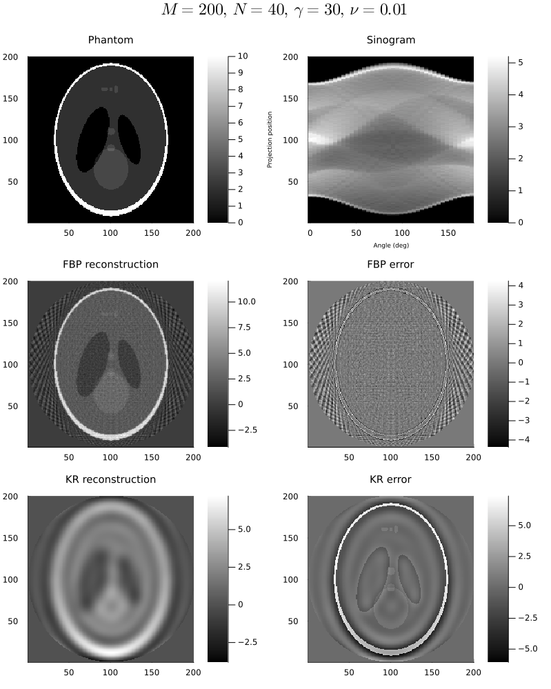
Figure 6: Reconstructions of an ideal sinogram (top right) at $N=40$ equidistant angles over $[-\pi/2,\pi/2)$ (rad), generated by the $M\times M$ ($M=200$) pixelated 2D Shepp-Logan phantom (top left). The Gaussian kernel with $\gamma=30$ and the penalty level $\nu=0.1$ in Theorem 3.9 was used for the kernel reconstruction (bottom left).

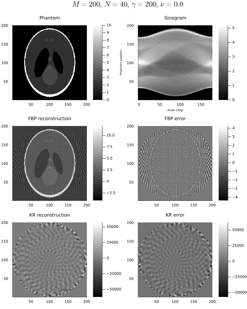
Figure 7: Reconstructions of an ideal sinogram (top right) at $N=40$ equidistant angles over $[-\pi/2,\pi/2)$ (rad), generated by the $M\times M$ ($M=200$) pixelated 2D Shepp-Logan phantom (top left). The Gaussian kernel $\gamma=200$ in Theorem 3.8 was used for the kernel MLE reconstruction (bottom left) without the penalty.

Appendix E Proofs of theorems

E.1 Proof in Section 2

Proof of Proposition 2.5.

For $f\in\mathcal{L}_{2}(\mathbb{R}^{n})$, by the Cauchy-Schwarz inequality,

$$\|\mathscr{P}_{R}f\|^{2}_{\mathcal{L}_{2}}= \int_{\mathbb{B}^{n-1}}\lvert\mathscr{P}_{R}f(\mathbf{x})\rvert^{2}\mathrm{d}\mathbf{x}=\int_{\mathbb{B}^{n-1}}\bigg{\lvert}\int_{I_{\|\mathbf{x}\|}}f(R^{\top}[\mathbf{x}:z])\mathrm{d}z\bigg{\rvert}^{2}\mathrm{d}\mathbf{x}$$

$$\leq \int_{\mathbb{B}^{n-1}}2W(\mathbf{x})\int_{I_{\|\mathbf{x}\|}}\lvert f(R^{\top}[\mathbf{x}:z])\rvert^{2}\mathrm{d}z\mathrm{d}\mathbf{x}$$

$$\leq 2\int_{\mathbb{B}^{n-1}}\int_{I_{\|\mathbf{x}\|}}\lvert f(R^{\top}[\mathbf{x}:z])\rvert^{2}\mathrm{d}z\mathrm{d}\mathbf{x}=2\int_{\mathbb{B}^{n}}\lvert f(\mathbf{z})\rvert^{2}\mathrm{d}\mathbf{z}=2\|f\|^{2}_{\mathcal{L}_{2}},$$

where we have put $\mathbf{z}=R^{\top}[\mathbf{x}:z]$ so that $\mathrm{d}\mathbf{z}=\mathrm{d}\mathbf{x}\mathrm{d}z$. Similarly,

$$\|\mathscr{P}f\|^{2}_{\mathcal{L}_{2}}=\int_{SO(n)}\int_{\mathbb{B}^{n-1}}\lvert\mathscr{P}f(R,\mathbf{x})\rvert^{2}\mathrm{d}\mathbf{x}\mathrm{d}R\leq\int_{SO(n)}2\|f\|^{2}_{\mathcal{L}_{2}}\mathrm{d}R=2\|f\|^{2}_{\mathcal{L}_{2}}.$$

To calculate the adjoint operator, let $f\in\mathcal{L}_{2}(\mathbb{B}^{n})$ and $g\in\mathcal{L}_{2}(\mathbb{B}^{n-1})$. Then

$$\langle f,\mathscr{P}_{R}^{*}g\rangle_{\mathcal{L}_{2}}= \langle\mathscr{P}_{R}f,g\rangle_{\mathcal{L}_{2}}=\int_{\mathbb{B}^{n-1}}\mathscr{P}_{R}f(\mathbf{x})g(\mathbf{x})\mathrm{d}\mathbf{x}$$

$$= \int_{\mathbb{B}^{n-1}}\int_{I_{\|\mathbf{x}\|}}f(R^{\top}[\mathbf{x}:z])g(\mathbf{x})\mathrm{d}z\mathrm{d}\mathbf{x}=\int_{\mathbb{B}^{n}}f(\mathbf{z})g(\mathbf{P}_{R}(\mathbf{z}))\mathrm{d}\mathbf{z},$$

where we have put $\mathbf{z}=R^{\top}[\mathbf{x}:z]$ so that $\mathbf{x}=\mathbf{P}_{R}(\mathbf{z})$. Similarly, for $g\in\mathcal{L}_{2}(SO(n)\times\mathbb{B}^{n-1})$,

$$\langle f,\mathscr{P}^{*}g\rangle_{\mathcal{L}_{2}}=\langle\mathscr{P}_{R}f,g\rangle_{\mathcal{L}_{2}}= \int_{SO(n)}\int_{\mathbb{B}^{n-1}}\mathscr{P}_{R}f(\mathbf{x})g(R,\mathbf{x})\mathrm{d}\mathbf{x}\mathrm{d}R$$

$$= \int_{SO(n)}\int_{\mathbb{B}^{n-1}}\int_{I_{\|\mathbf{x}\|}}f(R^{\top}[\mathbf{x}:z])g(R,\mathbf{x})\mathrm{d}z\mathrm{d}\mathbf{x}\mathrm{d}R$$

$$= \int_{\mathbb{B}^{n}}f(\mathbf{z})\left(\int_{SO(n)}g(R,\mathbf{P}_{R}(\mathbf{z}))\mathrm{d}R\right)\mathrm{d}\mathbf{z}.$$

∎

Proof of Theorem 2.7.

For any $\eta\in\mathbb{R}^{n-1}$,

$$\widehat{\mathscr{P}_{R}f}(\eta)= (2\pi)^{-(n-1)/2}\int_{\mathbb{R}^{n-1}}e^{-\imath\mathbf{x}^{\top}\eta}\mathscr{P}_{R}f(\mathbf{x})\mathrm{d}\mathbf{x}$$

$$= (2\pi)^{-(n-1)/2}\int_{\mathbb{R}^{n-1}}e^{-\imath\mathbf{x}^{\top}\eta}\int_{-\infty}^{+\infty}f(R^{\top}[\mathbf{x}:z])\mathrm{d}z\mathrm{d}\mathbf{x}$$

$$= (2\pi)^{-(n-1)/2}\int_{\mathbb{R}^{n}}e^{-\imath\mathbf{z}^{\top}R^{\top}[\eta:0]}f(\mathbf{z})\mathrm{d}\mathbf{z}=\sqrt{2\pi}\hat{f}(R^{\top}[\eta:0]),$$

where we have put $\mathbf{z}=R^{\top}[\mathbf{x}:z]$. ∎

Proof of Theorem 2.8.

By the Fourier inversion formula and Proposition B.3,

$$\mathscr{I}^{\alpha}f(\mathbf{z})= (2\pi)^{-n/2}\int_{\mathbb{R}^{n}}e^{\imath\mathbf{z}^{\top}\xi}|\xi|^{-\alpha}\hat{f}(\xi)\mathrm{d}\xi$$

$$= (2\pi)^{-n/2}\frac{|\mathbb{S}^{n-1}|}{|\mathbb{S}^{n-2}|}\int_{SO(n)}\int_{\mathbb{R}^{n-1}}e^{\imath\mathbf{z}^{\top}R^{\top}[\eta:0]}|\eta|^{1-\alpha}\hat{f}(R^{\top}[\eta:0])\mathrm{d}\eta\mathrm{d}R.$$

Note that $\mathbf{z}^{\top}R^{\top}[\eta:0]=(R\mathbf{z})^{\top}[\eta:0]=\mathbf{P}_{R}(\mathbf{z})^{\top}\eta$. Thus, by Propositions B.3, 2.7 and 2.5,

$$\mathscr{I}^{\alpha}f(\mathbf{z})= (2\pi)^{-(n+1)/2}\frac{|\mathbb{S}^{n-1}|}{|\mathbb{S}^{n-2}|}\int_{SO(n)}\int_{\mathbb{R}^{n-1}}e^{\imath\mathbf{P}_{R}(\mathbf{z})^{\top}\eta}|\eta|^{1-\alpha}\widehat{\mathscr{P}_{R}f}(\eta)\mathrm{d}\eta\mathrm{d}R$$

$$= \frac{|\mathbb{S}^{n-1}|}{2\pi|\mathbb{S}^{n-2}|}\int_{SO(n)}|\eta|^{1-\alpha}(\widehat{\mathscr{P}_{R}f})\check{}(\mathbf{P}_{R}(\mathbf{z}))\mathrm{d}R$$

$$= \frac{|\mathbb{S}^{n-1}|}{2\pi|\mathbb{S}^{n-2}|}\int_{SO(n)}\mathscr{I}^{\alpha-1}\mathscr{P}f(R,\mathbf{P}_{R}(\mathbf{z}))\mathrm{d}R$$

$$= \frac{|\mathbb{S}^{n-1}|}{2\pi|\mathbb{S}^{n-2}|}\mathscr{P}^{*}\mathscr{I}^{\alpha-1}\mathscr{P}f(\mathbf{z}).$$

∎

E.2 Proofs in Section 3

Proof of Proposition 3.3.

Given distinct points $\mathbf{x}_{i}\in\mathbb{B}^{n-1}$ and given $\alpha_{i}\in\mathbb{C}$ for $1\leq i\leq M$,

$$\sum_{i,j=1}^{M}\overline{\alpha_{i}}\alpha_{j} \tilde{K}^{R}(\mathbf{x}_{i},\mathbf{x}_{j})=\sum_{i,j=1}^{M}\overline{\alpha_{i}}\alpha_{j}\int_{I_{\|\mathbf{x}_{j}\|}}\int_{I_{\|\mathbf{x}_{i}\|}}K(R^{\top}[\mathbf{x}_{i}:z_{1}],R^{\top}[\mathbf{x}_{j}:z_{2}])\mathrm{d}z_{1}\mathrm{d}z_{2}$$

$$= \int_{-1}^{+1}\int_{-1}^{+1}\left(\sum_{i,j=1}^{M}\overline{\alpha_{i}}\alpha_{j}K(R^{\top}[\mathbf{x}_{i}:z_{1}],R^{\top}[\mathbf{x}_{j}:z_{2}])\right)\mathrm{d}z_{1}\mathrm{d}z_{2}\geq 0,$$

since the integrand is always nonnegative, thus $\tilde{K}^{R}$ is also a kernel. Also, equality holds if and only if the integrand is always 0. Thus, if $\mathbf{x}_{1},\mathbf{x}_{2},\dots,\mathbf{x}_{M}\in(\mathbb{B}^{n-1})^{\circ}$ and $\tilde{K}^{R}$ is strictly p.d., then equality holds if and only if $\alpha_{1}=\dots=\alpha_{M}=0$. This entails that the restriction of $\tilde{K}^{R}$ to $(\mathbb{B}^{n-1})^{\circ}$ is strictly p.d, provided that $K$ is strictly p.d.

Let $K:\mathbb{B}^{n}\times\mathbb{B}^{n}\rightarrow\mathbb{R}$ be continuous. Then, it is uniformly continuous due to the compactness of $\mathbb{B}^{n}$, so for any $\varepsilon>0$, there is some $\delta>0$ such that $\|(\mathbf{z}_{1},\mathbf{z}_{2})-(\mathbf{z}_{1}^{{}^{\prime}},\mathbf{z}_{2}^{{}^{\prime}})\|<\delta$ implies $|K(\mathbf{z}_{1},\mathbf{z}_{2})-K(\mathbf{z}_{1}^{{}^{\prime}},\mathbf{z}_{2}^{{}^{\prime}})|<\varepsilon$. Then, whenever $\|(\mathbf{x}_{1},\mathbf{x}_{2})-(\mathbf{x}_{1}^{{}^{\prime}},\mathbf{x}_{2}^{{}^{\prime}})\|<\delta$, we obtain

$$\left|\tilde{K}^{R}(\mathbf{x}_{1},\mathbf{x}_{2})-\tilde{K}^{R}(\mathbf{x}_{1}^{{}^{\prime}},\mathbf{x}_{2}^{{}^{\prime}})\right|$$

$$\leq\int_{-1}^{+1}\int_{-1}^{+1}\left|K(R^{\top}[\mathbf{x}_{1}:z_{1}],R^{\top}[\mathbf{x}_{2}:z_{2}])-K(R^{\top}[\mathbf{x}_{1}^{{}^{\prime}}:z_{1}],R^{\top}[\mathbf{x}_{2}^{{}^{\prime}}:z_{2}])\right|\mathrm{d}z_{1}\mathrm{d}z_{2}$$

$$\leq 4\varepsilon,$$

hence $\tilde{K}^{R}$ is also uniformly continuous. ∎

To prove our central theorem (Theorem 3.4) that constitutes our framework, we use the following lemma, of which the proof can be found in Theorem 3.11 of [22].

Lemma E.1.

Let $\mathbb{H}(K)$ be the RKHS on $E$ with a reproducing kernel $K$. Then $f\in\mathbb{H}(K)$ if and only if there exists a constant $c\geq 0$ such that $c^{2}K(x,y)-f(x)\overline{f(y)}$ is a kernel function. Moreover, if $f\in\mathbb{H}(K)$, then $\|f\|_{\mathbb{H}(K)}$ is the least $c$ that satisfies the statement above.

Theorem E.2.

For any $R\in SO(n)$,

1. $\mathscr{P}_{R}:\mathbb{H}(K)\rightarrow\mathbb{H}(\tilde{K}^{R})$ is a contractive, surjective, linear map.

2. For $g\in\mathbb{H}(\tilde{K}^{R})$, we have $\|g\|_{\mathbb{H}(\tilde{K}^{R})}=\min\left\{\|f\|_{\mathbb{H}(K)}:g=\mathscr{P}_{R}f\right\}$.

Proof.

First, we show that if $f\in\mathbb{H}(K)$, then $\mathscr{P}_{R}f\in\mathbb{H}(\tilde{K}^{R})$. Let $\|f\|_{\mathbb{H}(K)}=c$. By Lemma E.1, $\hat{K}(\mathbf{z}_{1},\mathbf{z}_{2}):=c^{2}K(\mathbf{z}_{1},\mathbf{z}_{2})-f(\mathbf{z}_{1})\overline{f(\mathbf{z}_{2})}$ is a kernel function on $\mathbb{B}^{n}$. Note that for any $\mathbf{x}_{1},\mathbf{x}_{2},\dots,\mathbf{x}_{M}\in\mathbb{B}^{n-1}$ and $\alpha_{1},\alpha_{2},\dots,\alpha_{M}\in\mathbb{C}$,

$$\sum_{i,j=1}^{M}\overline{\alpha_{i}}\alpha_{j}\left(c^{2}\tilde{K}^{R}(\mathbf{x}_{1},\mathbf{x}_{2})-\mathscr{P}_{R}f(\mathbf{x}_{1})\overline{\mathscr{P}_{R}f(\mathbf{x}_{2})}\right)$$

$$= \sum_{i,j=1}^{M}\overline{\alpha_{i}}\alpha_{j}\int_{I_{\|\mathbf{x}_{j}\|}}\int_{I_{\|\mathbf{x}_{i}\|}}\hat{K}(R^{\top}[\mathbf{x}_{i}:z_{1}],R^{\top}[\mathbf{x}_{j}:z_{2}])\mathrm{d}z_{1}\mathrm{d}z_{2}$$

$$= \int_{-1}^{+1}\int_{-1}^{+1}\left(\sum_{i,j=1}^{M}\overline{\alpha_{i}}\alpha_{j}\hat{K}(R^{\top}[\mathbf{x}_{i}:z_{1}],R^{\top}[\mathbf{x}_{j}:z_{2}])\right)\mathrm{d}z_{1}\mathrm{d}z_{2}\geq 0,$$

since the integrand is always non-negative. Hence, $\hat{K}^{R}(\mathbf{x}_{1},\mathbf{x}_{2}):=c^{2}\tilde{K}^{R}(\mathbf{x}_{1},\mathbf{x}_{2})-\mathscr{P}_{R}f(\mathbf{x}_{1})\overline{\mathscr{P}_{R}f(\mathbf{x}_{2})}$ is a kernel on $\mathbb{B}^{n-1}$, and by Lemma E.1 again, we get $\mathscr{P}_{R}f\in\mathbb{H}(\tilde{K}^{R})$ with $\|\mathscr{P}_{R}f\|_{\mathbb{H}(\tilde{K}^{R})}\leq\|f\|_{\mathbb{H}(K)}$, i.e. $\mathscr{P}_{R}:\mathbb{H}(K)\rightarrow\mathbb{H}(\tilde{K}^{R})$ is a contractive linear map.

To establish surjectivity, let $\mathbb{V}(\tilde{K}^{R})$ denote the vector space of functions spanned by $\{\tilde{k}^{R}_{\mathbf{x}}:\mathbf{x}\in\mathbb{B}^{n-1}\}$. For any $\mathbf{x}_{1},\dots,\mathbf{x}_{M}\in\mathbb{B}^{n-1}$ and $\alpha_{1},\dots,\alpha_{M}\in\mathbb{F}$ $(=\mathbb{R}\text{ or }\mathbb{C})$,

$$\left\|\sum_{i=1}^{M}\alpha_{i}\tilde{k}^{R}_{\mathbf{x}_{i}}\right\|^{2}_{\mathbb{H}(\tilde{K}^{R})}= \sum_{i,j=1}^{M}\overline{\alpha_{i}}\alpha_{j}\int_{I_{\|\mathbf{x}_{j}\|}}\int_{I_{\|\mathbf{x}_{i}\|}}K(R^{\top}[\mathbf{x}_{i}:z_{1}],R^{\top}[\mathbf{x}_{j}:z_{2}])\mathrm{d}z_{1}\mathrm{d}z_{2}$$

$$= \int_{-1}^{+1}\int_{-1}^{+1}\sum_{i,j=1}^{M}\overline{\alpha_{i}}\alpha_{j}\langle k_{R^{\top}[\mathbf{x}_{i}:z_{1}]},k_{R^{\top}[\mathbf{x}_{j}:z_{2}]}\rangle_{\mathbb{H}(K)}\mathrm{d}z_{1}\mathrm{d}z_{2}$$

$$= \left\|\sum_{i=1}^{M}\alpha_{i}\int_{I_{\|\mathbf{x}_{i}\|}}k_{R^{\top}[\mathbf{x}_{i}:z]}\mathrm{d}z\right\|^{2}_{\mathbb{H}(K)},$$

in the sense of the Bochner integration. Therefore, there is a well-defined isometry (injective, but not necessarily surjective) $\mathbf{\Gamma}_{R}:\mathbb{V}(\tilde{K}^{R})\rightarrow\mathbb{H}(K)$ given by

$$\mathbf{\Gamma}_{R}\left(\sum_{i=1}^{n}\alpha_{i}\tilde{k}^{R}_{\mathbf{x}_{i}}\right):=\sum_{i=1}^{n}\alpha_{i}\int_{I_{\|\mathbf{x}_{i}\|}}k_{R^{\top}[\mathbf{x}_{i}:z]}\mathrm{d}z,$$

and it induces a unique isometric extension $\mathbf{\Gamma}_{R}:\mathbb{H}(\tilde{K}^{R})\rightarrow\mathbb{H}(K)$ since $\mathbb{V}(\tilde{K}^{R})$ forms a dense subspace of $\mathbb{H}(\tilde{K}^{R})$. Additionally, for any induced generator $\tilde{k}^{R}_{\mathbf{x}_{1}}$ at $\mathbf{x}_{1}\in\mathbb{B}^{n-1}$ and any point $\mathbf{x}_{2}\in\mathbb{B}^{n-1}$,

$$(\mathscr{P}_{R}\circ\mathbf{\Gamma}_{R})(\tilde{k}^{R}_{\mathbf{x}_{1}})(\mathbf{x}_{2})= \int_{I_{\|\mathbf{x}_{2}\|}}\mathbf{\Gamma}_{R}(\tilde{k}^{R}_{\mathbf{x}_{1}})(R^{\top}[\mathbf{x}_{2}:z_{2}])\mathrm{d}z_{2}$$

$$= \int_{I_{\|\mathbf{x}_{2}\|}}\int_{I_{\|\mathbf{x}_{1}\|}}k_{R^{\top}[\mathbf{x}_{1}:z_{1}]}(R^{\top}[\mathbf{x}_{2}:z_{2}])\mathrm{d}z_{1}\mathrm{d}z_{2}$$

$$= \int_{I_{\|\mathbf{x}_{2}\|}}\int_{I_{\|\mathbf{x}_{1}\|}}K(R^{\top}[\mathbf{x}_{2}:z_{2}],R^{\top}[\mathbf{x}_{1}:z_{1}])\mathrm{d}z_{1}\mathrm{d}z_{2}$$

$$= \tilde{K}^{R}(\mathbf{x}_{2},\mathbf{x}_{1})=\tilde{k}^{R}_{\mathbf{x}_{1}}(\mathbf{x}_{2}),$$

because the convergence in RKHS implies pointwise convergence. Since $\mathbb{V}(\tilde{K}^{R})$ is dense in $\mathbb{H}(\tilde{K}^{R})$, the above equation shows that $\mathscr{P}_{R}\circ\mathbf{\Gamma}_{R}$ is the identity map on $\mathbb{H}(\tilde{K}^{R})$. Therefore, for any $g\in\mathbb{H}(\tilde{K}^{R})$, the function $f=\mathbf{\Gamma}_{R}(g)\in\mathbb{H}(K)$ satisfies $g=\mathscr{P}_{R}f$, which shows the surjectivity of $\mathscr{P}_{R}:\mathbb{H}(K)\rightarrow\mathbb{H}(\tilde{K}^{R})$. Finally, we obtain $\|g\|_{\mathbb{H}(\tilde{K}^{R})}=\|\mathbf{\Gamma}_{R}(g)\|_{\mathbb{H}(K)}=\min\left\{\|f\|_{\mathbb{H}(K)}:g=\mathscr{P}_{R}f\right\}$. ∎

As can be seen in Theorem E.2, $\mathscr{P}_{R}:\mathbb{H}(K)\rightarrow\mathbb{H}(\tilde{K}^{R})$ is contractive, meaning its operator norm is at most 1. This naturally prompts the question of its adjoint operator. Interestingly, the isometry $\mathbf{\Gamma}_{R}:\mathbb{H}(\tilde{K}^{R})\rightarrow\mathbb{H}(K)$ serves as the adjoint operator of $\mathscr{P}_{R}$ for any $R\in SO(n)$. Since the adjoint operator $\mathbf{\Gamma}_{R}$ is isometric, its range forms a closed subspace of $\mathbb{H}(K)$, and thus itself becomes a Hilbert space.

Proposition E.3.

Let $R\in SO(n)$ and $\mathbb{H}_{R}(K):=\{\mathbf{\Gamma}_{R}g:g\in\mathbb{H}(\tilde{K}^{R})\}$.

1. Any $f\in\mathbb{H}(K)$ can be uniquely expressed as a direct sum:

   $$f=(\mathbf{\Gamma}_{R}\circ\mathscr{P}_{R})f\oplus(f-(\mathbf{\Gamma}_{R}\circ\mathscr{P}_{R})f)\in\mathbb{H}_{R}(K)\oplus(\mathbb{H}_{R}(K))^{\perp},$$

   thus $f\in\mathbb{H}_{R}(K)$ if and only if $f=(\mathbf{\Gamma}_{R}\circ\mathscr{P}_{R})f$.

2. $(\mathbb{H}_{R}(K))^{\perp}=\mathcal{N}(\mathscr{P}_{R}),\ \mathbb{H}_{R}(K)=(\mathcal{N}(\mathscr{P}_{R}))^{\perp}$.

Proof.

1. It suffices to show that for any $f\in\mathbb{H}(K)$, $g\in\mathbb{H}(\tilde{K}^{R})$, $\langle\mathbf{\Gamma}_{R}g,(f-(\mathbf{\Gamma}_{R}\circ\mathscr{P}_{R})f)\rangle_{\mathbb{H}(K)}=0$. Given $t\in\mathbb{R}$, let $h=\mathbf{\Gamma}_{R}g+t(f-(\mathbf{\Gamma}_{R}\circ\mathscr{P}_{R})f)\in\mathbb{H}(K)$. Note that $\mathscr{P}_{R}h=g$. Since $\mathscr{P}_{R}:\mathbb{H}(K)\rightarrow\mathbb{H}(\tilde{K}^{R})$ is contractive and $\mathbf{\Gamma}_{R}:\mathbb{H}(\tilde{K}^{R})\rightarrow\mathbb{H}(K)$ is isometric, we have for any $t\in\mathbb{R}$,

   $$0 \leq\|h\|^{2}_{\mathbb{H}(K)}-\|\mathscr{P}_{R}h\|^{2}_{\mathbb{H}(\tilde{K}^{R})}$$

   $$=2t\langle\mathbf{\Gamma}_{R}g,(f-(\mathbf{\Gamma}_{R}\circ\mathscr{P}_{R})f)\rangle_{\mathbb{H}(K)}+t^{2}\|(f-(\mathbf{\Gamma}_{R}\circ\mathscr{P}_{R})f)\|^{2}_{\mathbb{H}(K)},$$

   which reveals that $\langle\mathbf{\Gamma}_{R}g,(f-(\mathbf{\Gamma}_{R}\circ\mathscr{P}_{R})f)\rangle_{\mathbb{H}(K)}=0$.

2. By (1) and the fact that $\mathscr{P}_{R}\circ\mathbf{\Gamma}_{R}$ is the identity map on $\mathbb{H}(\tilde{K}^{R})$,

   $$f\in\mathcal{N}(\mathscr{P}_{R})\Longleftrightarrow\mathscr{P}_{R}f=0\Longleftrightarrow(\mathbf{\Gamma}_{R}\circ\mathscr{P}_{R})f=0\Longleftrightarrow f\in(\mathbb{H}_{R}(K))^{\perp}.$$

   Hence, $(\mathbb{H}_{R}(K))^{\perp}=\mathcal{N}(\mathscr{P}_{R})$. Also, we get $\mathbb{H}_{R}(K)=(\mathcal{N}(\mathscr{P}_{R}))^{\perp}$ as $\mathbb{H}_{R}(K)$ is closed.

∎

Corollary E.4.

For any $R\in SO(n)$, $\mathscr{P}_{R}^{*}=\mathbf{\Gamma}_{R}:\mathbb{H}(\tilde{K}^{R})\rightarrow\mathbb{H}(K)$. The adjoint operator is uniquely determined by

$$\mathscr{P}_{R}^{*}(\tilde{k}^{R}_{\mathbf{x}})=\int_{I_{\|\mathbf{x}\|}}k_{R^{\top}[\mathbf{x}:z]}\mathrm{d}z,\quad\mathbf{x}\in\mathbb{B}^{n-1},$$

or equivalently, $\mathscr{P}_{R}^{*}(\tilde{k}^{R}_{\mathbf{x}})(\mathbf{z})=\int_{I_{\|\mathbf{x}\|}}K(\mathbf{z},R^{\top}[\mathbf{x}:z])\mathrm{d}z$ for any $\mathbf{x}\in\mathbb{B}^{n-1},\mathbf{z}\in\mathbb{B}^{n}$.

Proof.

Given $f\in\mathbb{H}(K)$, there are unique $g_{1}\in\mathbb{H}(\tilde{K}^{R})$ and $f_{1}\in(\mathbb{H}_{R}(K))^{\perp}$ such that $f=\mathbf{\Gamma}_{R}g_{1}\oplus f_{1}\in\mathbb{H}_{R}(K)\oplus(\mathbb{H}_{R}(K))^{\perp}$. Then for any $g\in\mathbb{H}(\tilde{K}^{R})$, by the proof of Theorem E.2 and Proposition E.3,

$$\langle f,\mathscr{P}_{R}^{*}g\rangle_{\mathbb{H}(K)}=\langle\mathscr{P}_{R}f,g\rangle_{\mathbb{H}(\tilde{K}^{R})}=\langle g_{1},g\rangle_{\mathbb{H}(\tilde{K}^{R})}=\langle\mathbf{\Gamma}_{R}g_{1},\mathbf{\Gamma}_{R}g\rangle_{\mathbb{H}(K)}=\langle f,\mathbf{\Gamma}_{R}g\rangle_{\mathbb{H}(K)}.$$

Since $f\in\mathbb{H}(K)$ and $g\in\mathbb{H}(\tilde{K}^{R})$ were chosen arbitrarily, we have $\mathscr{P}_{R}^{*}=\mathbf{\Gamma}_{R}:\mathbb{H}(\tilde{K}^{R})\rightarrow\mathbb{H}(K)$. ∎

Theorem E.2, Proposition E.3, and Corollary E.4 collectively prove the Theorem 3.4.

Proof of Proposition 3.5.

1. $\langle\mathscr{P}_{R}f,k^{R}_{\mathbf{x}_{k}}\rangle_{\mathbb{H}(\tilde{K}^{R})}=\mathscr{P}_{R}f(\mathbf{x}_{k})=0$ for all $k=1,\dots,M$ if and only if $\mathscr{P}_{R}f\in(\mathbb{V}_{\mathbf{F}}(\tilde{K}^{R}))^{\perp}$, which is equivalent to $f\in\mathscr{P}^{-1}_{R}((\mathbb{V}_{\mathbf{F}}(\tilde{K}^{R}))^{\perp})$.

2. First, note that $(\mathbb{V}_{\mathbf{F}}(\tilde{K}^{R}))^{\perp}$ is closed, thus so is $\mathscr{P}^{-1}_{R}((\mathbb{V}_{\mathbf{F}}(\tilde{K}^{R}))^{\perp})$. Now, for any $f\in\mathbb{H}(K)$, let $f=\mathscr{P}_{R}^{*}g+f^{{}^{\prime}}\in\mathbb{H}_{R}(K)\oplus\mathcal{N}(\mathscr{P}_{R})$ be its decomposition as in Theorem 3.4. Then, $f\in\mathscr{P}^{-1}_{R}((\mathbb{V}_{\mathbf{F}}(\tilde{K}^{R}))^{\perp})$ if and only if $g=\mathscr{P}_{R}f\in(\mathbb{V}_{\mathbf{F}}(\tilde{K}^{R}))^{\perp}$.

3. From (2) and Theorem 3.4,

   $$(\mathscr{P}^{-1}_{R}((\mathbb{V}_{\mathbf{F}}(\tilde{K}^{R}))^{\perp}))^{\perp}= [\mathscr{P}_{R}^{*}((\mathbb{V}_{\mathbf{F}}(\tilde{K}^{R}))^{\perp})\oplus\mathcal{N}(\mathscr{P}_{R})]^{\perp}$$

   $$= [\mathscr{P}_{R}^{*}((\mathbb{V}_{\mathbf{F}}(\tilde{K}^{R}))^{\perp})]^{\perp}\cap\mathbb{H}_{R}(K)$$

   $$= [\mathscr{P}_{R}^{*}((\mathbb{V}_{\mathbf{F}}(\tilde{K}^{R}))^{\perp})]^{\perp}\cap\mathscr{P}_{R}^{*}(\mathbb{H}(K))=\mathscr{P}_{R}^{*}(\mathbb{V}_{\mathbf{F}}(\tilde{K}^{R})),$$

   where we have used the fact that $\mathscr{P}_{R}^{*}:\mathbb{H}(\tilde{K}^{R})\rightarrow\mathbb{H}(K)$ is an isometry for the last equality. Indeed, $\mathscr{P}_{R}^{*}(\mathbb{V}_{\mathbf{F}}(\tilde{K}^{R}))$ is a closed subspace of $\mathbb{H}(K)$.

∎

Proof of Proposition 3.6.

The first part of the statement and (12) are straightforward from (10). Let us show that if $K:\mathbb{B}^{n}\times\mathbb{B}^{n}\rightarrow\mathbb{R}$ is strictly p.d. and $\mathbf{F}=\{\mathbf{x}_{1},\dots,\mathbf{x}_{M}\}\subset(\mathbb{B}^{n-1})^{\circ}$, then $\mathbf{W}\in\mathbb{R}^{NM\times NM}$ is also strictly p.d.. Suppose $\boldsymbol{\alpha}^{\top}\mathbf{W}\boldsymbol{\alpha}=0$. By (11),

$$0 =\boldsymbol{\alpha}^{\top}\mathbf{W}\boldsymbol{\alpha}=\sum_{i,i^{\prime}=1}^{N}\sum_{j,j^{\prime}=1}^{M}\alpha_{ij}\alpha_{i^{\prime}j^{\prime}}w_{ij,i^{\prime}j^{\prime}}$$

$$=\int_{-1}^{+1}\int_{-1}^{+1}\left(\sum_{i,i^{\prime}=1}^{N}\sum_{j,j^{\prime}=1}^{M}\alpha_{ij}\alpha_{i^{\prime}j^{\prime}}K(R_{i}^{\top}[\mathbf{x}_{j}:z_{1}],R_{i^{\prime}}^{\top}[\mathbf{x}_{j^{\prime}}:z_{2}])\right)\mathrm{d}z_{1}\mathrm{d}z_{2}\geq 0.$$

Because the integrand is always nonnegative, equality holds if and only if the integrand is always 0. Since $K$ is strictly p.d and $\|\mathbf{x}_{j}\|<1$ for all $j=1,\dots,M$, we obtain $\boldsymbol{\alpha}=0$, i.e. $\mathbf{W}$ is strictly p.d.. ∎

Proof of Theorem 3.8.

For (1), note that any solution of (13) belongs to the set $\mathbf{W}^{\dagger}\mathbf{Y}\oplus\mathcal{N}(\mathbf{W})$ since $\mathbf{W}^{\dagger}\mathbf{Y}=\mathbf{W}(\mathbf{W}^{\dagger})^{2}\mathbf{Y}\in\mathcal{R}(\mathbf{W})=(\mathcal{N}(\mathbf{W}))^{\perp}$, thus $\hat{\boldsymbol{\alpha}}^{0}:=\mathbf{W}^{\dagger}\mathbf{Y}\in\mathcal{R}(\mathbf{W})$ is the minimizer with the minimum norm. Also, by (9), $\hat{f}^{0}=(\mathcal{I}^{\mathbf{R}}_{\mathbf{F}})^{-1}(\mathbf{W}\hat{\boldsymbol{\alpha}}^{0})$ is the minimizer with the minimum norm. For (2), repeat the argument with $\mathbf{Y}$ replaced by $\mathbf{W}\boldsymbol{\alpha}^{0}$. For (3), $\hat{\boldsymbol{\alpha}}^{0}=\mathbf{W}^{\dagger}\mathbf{Y}\sim N(\mathbf{W}\mathbf{W}^{\dagger}\boldsymbol{\alpha}^{0},\sigma^{2}(\mathbf{W}^{\dagger})^{2})$ since $\mathbf{Y}\sim N(\mathbf{W}\boldsymbol{\alpha}^{0},\sigma^{2}\mathbf{I})$. Also, by the isometry in (12), for any $f\in\mathbb{H}^{\mathbf{R}}_{\mathbf{F}}$,

$$\text{Cov}(\hat{f}^{0})f =\mathbb{E}[(\hat{f}^{0}-\mathbb{E}[\hat{f}^{0}])\cdot\langle\hat{f}^{0}-\mathbb{E}[\hat{f}^{0}],f\rangle_{\mathbb{H}(K)}]$$

$$=\mathbb{E}[(\mathcal{I}^{\mathbf{R}}_{\mathbf{F}})^{-1}(\mathbf{W}(\hat{\boldsymbol{\alpha}}^{0}-\mathbf{W}\mathbf{W}^{\dagger}\boldsymbol{\alpha}^{0}))\cdot\langle(\mathbf{W}(\hat{\boldsymbol{\alpha}}^{0}-\mathbf{W}\mathbf{W}^{\dagger}\boldsymbol{\alpha}^{0}),\mathcal{I}^{\mathbf{R}}_{\mathbf{F}}f\rangle_{\mathbf{W}}]$$

$$=\mathbb{E}[(\mathcal{I}^{\mathbf{R}}_{\mathbf{F}})^{-1}\mathbf{W}(\hat{\boldsymbol{\alpha}}^{0}-\mathbf{W}\mathbf{W}^{\dagger}\boldsymbol{\alpha}^{0}))\cdot(\hat{\boldsymbol{\alpha}}^{0}-\mathbf{W}\mathbf{W}^{\dagger}\boldsymbol{\alpha}^{0})^{\top}\mathcal{I}^{\mathbf{R}}_{\mathbf{F}}f]$$

$$=\sigma^{2}(\mathcal{I}^{\mathbf{R}}_{\mathbf{F}})^{-1}\circ\mathbf{W}^{\dagger}\circ(\mathcal{I}^{\mathbf{R}}_{\mathbf{F}})f,$$

hence $\hat{f}^{0}\sim N(\mathcal{P}_{\mathbf{F}}^{\mathbf{R}}f^{0},\sigma^{2}(\mathcal{I}^{\mathbf{R}}_{\mathbf{F}})^{-1}\circ\mathbf{W}^{\dagger}\circ(\mathcal{I}^{\mathbf{R}}_{\mathbf{F}}))$. ∎

Proof of Theorem 3.9.

(1) is a direct consequence of (14). (3) can be shown in a similar way as Theorem 3.8. For (4), note that $\lim_{\nu\downarrow 0}(\mathbf{W}+\nu\mathbf{I})^{-1}=\mathbf{W}^{\dagger}$ and use the fact that $\mathcal{I}^{\mathbf{R}}_{\mathbf{F}}:\mathbb{H}^{\mathbf{R}}_{\mathbf{F}}\rightarrow\mathcal{R}(\mathbf{W})$ is an isomorphism by (12). Finally, for (2),

$$\hat{L}^{\nu}(\hat{\boldsymbol{\alpha}}^{\nu}) =\|\mathbf{Y}-\mathbf{W}\hat{\boldsymbol{\alpha}}^{\nu}\|^{2}+\nu(\hat{\boldsymbol{\alpha}}^{\nu})^{\top}\mathbf{W}\hat{\boldsymbol{\alpha}}^{\nu}$$

$$=\mathbf{Y}^{\top}\left[(\mathbf{I}-\mathbf{W}(\mathbf{W}+\nu\mathbf{I})^{-1})^{2}+\nu\mathbf{W}(\mathbf{W}+\nu I)^{-2}\right]\mathbf{Y}$$

$$=\mathbf{Y}^{\top}\left[(\nu\mathbf{I})^{2}+\nu\mathbf{W}\right](\mathbf{W}+\nu\mathbf{I})^{-2}\mathbf{Y}=\nu\mathbf{Y}^{\top}(\mathbf{W}+\nu\mathbf{I})^{-1}\mathbf{Y}.$$

∎

Proof of Proposition 3.10.

The first part is trivial since

$$\mathscr{P}\hat{f}^{\nu}(R,\mathbf{x})=\langle\mathscr{P}_{R}\hat{f}^{\nu},\tilde{k}^{R}_{\mathbf{x}}\rangle_{\mathbb{H}(\tilde{K}^{R})}=\langle\mathscr{P}_{R}^{*}\tilde{k}^{R}_{\mathbf{x}},\hat{f}^{\nu}.\rangle_{\mathbb{H}(K)},$$

For the HLCC, by (4),

$$\int_{\mathbb{B}^{n-1}}(\mathbf{x}^{\top}\mathbf{y})^{l}\mathscr{P}\hat{f}^{\nu}(R,\mathbf{x})\mathrm{d}\mathbf{x} =\int_{\mathbb{B}^{n-1}}(\mathbf{x}^{\top}\mathbf{y})^{l}\langle\mathscr{P}_{R}^{*}\tilde{k}^{R}_{\mathbf{x}},\hat{f}^{\nu}\rangle_{\mathbb{H}(K)}\mathrm{d}\mathbf{x}$$

$$=\int_{\mathbb{B}^{n-1}}\int_{I_{\|\mathbf{x}\|}}(\mathbf{x}^{\top}\mathbf{y})^{l}\langle k_{R^{\top}[\mathbf{x}:z]},\hat{f}^{\nu}\rangle_{\mathbb{H}(K)}\mathrm{d}z\mathrm{d}\mathbf{x}$$

$$=\int_{\mathbb{B}^{n}}(\mathbf{z}^{\top}R^{\top}[\mathbf{y}:0])^{l}\langle k_{\mathbf{z}},\hat{f}^{\nu}\rangle_{\mathbb{H}(K)}\mathrm{d}\mathbf{z}=q_{l}^{\nu}(\mathbf{P}_{R}^{*}(\mathbf{y})),$$

where we have set $\mathbf{z}=R^{\top}[\mathbf{x}:z]$. ∎

Proof of Proposition 3.11.

Since $\hat{f}^{\nu}\in\mathbb{H}^{\mathbf{R}}_{\mathbf{F}}$, by (9) and Proposition 3.6, we get

$$\mathbb{E}[ \|\hat{f}^{\nu}-f^{0}\|^{2}_{\mathbb{H}(K)}]=\mathbb{E}[\|\hat{f}^{\nu}-\mathcal{P}_{\mathbf{F}}^{\mathbf{R}}f^{0}\|^{2}_{\mathbb{H}(K)}]+\|f^{0}-\mathcal{P}_{\mathbf{F}}^{\mathbf{R}}f^{0}\|^{2}_{\mathbb{H}(K)}$$

$$= \mathbb{E}[(\hat{\boldsymbol{\alpha}}^{\nu}-\boldsymbol{\alpha}^{0})^{\top}\mathbf{W}(\hat{\boldsymbol{\alpha}}^{\nu}-\boldsymbol{\alpha}^{0})]+\|f^{0}-\mathcal{P}_{\mathbf{F}}^{\mathbf{R}}f^{0}\|^{2}_{\mathbb{H}(K)}.$$

Note that $(\hat{\boldsymbol{\alpha}}^{\nu}-\boldsymbol{\alpha}^{0})\sim N(-\nu(\mathbf{W}+\nu\mathbf{I})^{-1}\boldsymbol{\alpha}^{0},\sigma^{2}(\mathbf{W}+\nu\mathbf{I})^{-2})$ from Theorem 3.9, thus

$$\mathbb{E}[\|\hat{f}^{\nu}-f^{0}\|^{2}_{\mathbb{H}(K)}]$$

$$= \mathbb{E}[\hat{\boldsymbol{\alpha}}^{\nu}-\boldsymbol{\alpha}^{0}]^{\top}\mathbf{W}\mathbb{E}[\hat{\boldsymbol{\alpha}}^{\nu}-\boldsymbol{\alpha}^{0}]+\text{tr}(\mathbf{W}\text{Cov}[\hat{\boldsymbol{\alpha}}^{\nu}-\boldsymbol{\alpha}^{0}])+\|f^{0}-\mathcal{P}_{\mathbf{F}}^{\mathbf{R}}f^{0}\|^{2}_{\mathbb{H}(K)}$$

$$= \nu^{2}(\boldsymbol{\alpha}^{0})^{\top}\mathbf{W}(\mathbf{W}+\nu\mathbf{I})^{-2}\boldsymbol{\alpha}^{0}+\sigma^{2}\text{tr}(\mathbf{W}(\mathbf{W}+\nu\mathbf{I})^{-2})+\|f^{0}-\mathcal{P}_{\mathbf{F}}^{\mathbf{R}}f^{0}\|^{2}_{\mathbb{H}(K)}.$$

∎

Proof of Theorem 3.12.

By (9) and Proposition 3.6, we get

$$\|\hat{f}^{\nu}-f^{0}\|^{2}_{\mathbb{H}(K)}= \|\hat{f}^{\nu}-\mathcal{P}_{\mathbf{F}}^{\mathbf{R}}f^{0}\|^{2}_{\mathbb{H}(K)}+\|f^{0}-\mathcal{P}_{\mathbf{F}}^{\mathbf{R}}f^{0}\|^{2}_{\mathbb{H}(K)}$$

$$= (\hat{\boldsymbol{\alpha}}^{\nu}-\boldsymbol{\alpha}^{0})^{\top}\mathbf{W}(\hat{\boldsymbol{\alpha}}^{\nu}-\boldsymbol{\alpha}^{0})+\|f^{0}-\mathcal{P}_{\mathbf{F}}^{\mathbf{R}}f^{0}\|^{2}_{\mathbb{H}(K)}.$$

Let $\mathbf{W}=UDU^{\top}$ be the eigendecomposition of the Gram matrix, where $U\in O(NM)$ and $D=\text{diag}[d_{ij}]$. Denote $C(\nu):=(d+2\nu)^{-1}$, $\mathbf{v}:=U^{\top}(\mathbf{Y}-\mathbf{W}\boldsymbol{\alpha}^{0})\in\mathbb{R}^{NM}$ and $\mathbf{w}:=U^{\top}\boldsymbol{\alpha}^{0}\in\mathbb{R}^{NM}$. Due to (14), we obtain

$$(\hat{\boldsymbol{\alpha}}^{\nu}-\boldsymbol{\alpha}^{0})^{\top}\mathbf{W}(\hat{\boldsymbol{\alpha}}^{\nu}-\boldsymbol{\alpha}^{0})$$

$$= [(\mathbf{W}+\nu\mathbf{I})(\hat{\boldsymbol{\alpha}}^{\nu}-\boldsymbol{\alpha}^{0})]^{\top}[\mathbf{W}(\mathbf{W}+\nu\mathbf{I})^{-2}][(\mathbf{W}+\nu\mathbf{I})(\hat{\boldsymbol{\alpha}}^{\nu}-\boldsymbol{\alpha}^{0})]$$

$$= [(\mathbf{Y}-\mathbf{W}\boldsymbol{\alpha}^{0})-\nu\boldsymbol{\alpha}^{0}]^{\top}[\mathbf{W}(\mathbf{W}+\nu\mathbf{I})^{-2}][(\mathbf{Y}-\mathbf{W}\boldsymbol{\alpha}^{0})-\nu\boldsymbol{\alpha}^{0}]$$

$$= [\mathbf{v}-\nu\mathbf{w}]^{\top}[D(D+\nu D)^{-2}][\mathbf{v}-\nu\mathbf{w}]=\sum_{i=1}^{N}\sum_{j=1}^{M}\frac{d_{ij}}{(d_{ij}+\nu)^{2}}(v_{ij}-\nu w_{ij})^{2}$$

$$\leq C(\nu)\sum_{i=1}^{N}\sum_{j=1}^{M}v_{ij}^{2}+\sum_{i=1}^{N}\sum_{j=1}^{M}d_{ij}w_{ij}^{2}$$

$$= C(\nu)\|\mathbf{Y}-\mathbf{W}\boldsymbol{\alpha}^{0}\|^{2}+(\boldsymbol{\alpha}^{0})^{\top}\mathbf{W}\boldsymbol{\alpha}^{0}=C(\nu)\|\mathbf{Y}-\mathbf{W}\boldsymbol{\alpha}^{0}\|^{2}+\|\mathcal{P}_{\mathbf{F}}^{\mathbf{R}}f^{0}\|^{2}_{\mathbb{H}(K)},$$

where we have used the following quadratic equation for the inequality: for any $v,w\in\mathbb{R}$ and $d>0$, it holds that

$$(d+\nu)^{2}\left(\frac{v^{2}}{d+2\nu}+dw^{2}\right)-d(v-\nu w)^{2}$$

$$=\left[\frac{(d+\nu)^{2}}{d+2\nu}-d\right]v^{2}+2d\nu vw+d[(d+\nu)^{2}-\nu^{2}]w^{2}=\frac{[\nu v+d(d+2\nu)w]^{2}}{d+2\nu}\geq 0,$$

with equality if and only if $v=-d(d+2\nu)w/\nu$. Therefore,

$$\|\hat{f}^{\nu}-f^{0}\|^{2}_{\mathbb{H}(K)}\leq C(\nu)\|\mathbf{Y}-\mathbf{W}\boldsymbol{\alpha}^{0}\|^{2}+\|\mathcal{P}_{\mathbf{F}}^{\mathbf{R}}f^{0}\|^{2}_{\mathbb{H}(K)}+\|f^{0}-\mathcal{P}_{\mathbf{F}}^{\mathbf{R}}f^{0}\|^{2}_{\mathbb{H}(K)}$$

$$= \|f^{0}\|^{2}_{\mathbb{H}(K)}+C(\nu)\|\mathbf{Y}-\mathbf{W}\boldsymbol{\alpha}^{0}\|^{2}$$

$$= \|f^{0}\|^{2}_{\mathbb{H}(K)}+C(\nu)\sum_{i=1}^{N}\sum_{j=1}^{M}\varepsilon_{ij}^{2}.$$

Equality is achieved if $\mathbf{v}=-cd(d+2\nu)/\nu\,e_{IJ},\mathbf{w}=c\,e_{IJ}$ for any $c\in\mathbb{R}$ where the index $(I,J)$ is determined by $d_{IJ}=d>0$. In this case, $\|\mathcal{P}_{\mathbf{F}}^{\mathbf{R}}f^{0}\|^{2}_{\mathbb{H}(K)}=(\boldsymbol{\alpha}^{0})^{\top}\mathbf{W}\boldsymbol{\alpha}^{0}=\mathbf{w}^{\top}D\mathbf{w}=dc^{2}$, so we may take $c=\|\mathcal{P}_{\mathbf{F}}^{\mathbf{R}}f^{0}\|_{\mathbb{H}(K)}/\sqrt{d}$. ∎

E.3 Proofs in Section 4

Proof of Theorem 4.2.

Since $O(n)=SO(n)\rtimes\{I,J\}$, it suffices to show that $K(\mathbf{z}_{1},\mathbf{z}_{2})=K(J\mathbf{z}_{1},J\mathbf{z}_{2})$ for fixed $\mathbf{z}_{1},\mathbf{z}_{2}\in\mathbb{B}^{n}$. Let $\mathbf{z}_{i}=r_{i}\theta_{i}$ ($i=1,2$) be the polar decomposition with $r_{i}\in[0,1]$ and $\theta_{i}\in\mathbb{S}^{n-1}$, respectively. We may assume that $\theta_{1}=e_{n}$, since the left action of $SO(n)$ on $\mathbb{S}^{n-1}$ is transitive. Note that $J\mathbf{z}_{1}=-\mathbf{z}_{1}$, thus

$$K(J\mathbf{z}_{1},J\mathbf{z}_{2})=K(E(-e_{n})J\mathbf{z}_{1},E(-e_{n})J\mathbf{z}_{2})=K(\mathbf{z}_{1},\mathbf{z}^{\prime}_{2}),$$

where $\mathbf{z}^{\prime}_{2}:=E(-e_{n})J\mathbf{z}_{2}$. Let $\mathbf{z}^{\prime}_{2}=r_{2}\theta^{\prime}_{2}$ be the polar decomposition with $\theta^{\prime}_{i}\in\mathbb{S}^{n-1}$. We obtain

$$e_{n}^{\top}\mathbf{z}^{\prime}_{2}=e_{n}^{\top}E(-e_{n})J\mathbf{z}_{2}=(E(-e_{n})^{\top}e_{n})^{\top}J\mathbf{z}_{2}=-e_{n}^{\top}J\mathbf{z}_{2}=e_{n}^{\top}\mathbf{z}_{2}=:\cos\phi_{n-1},$$

for some $\phi_{n-1}\in[0,\pi]$, thus $\mathbf{z}_{2},\mathbf{z}^{\prime}_{2}\in\{r_{2}[\sin\phi_{n-1}\tilde{\theta}:\cos\phi_{n-1}]:\tilde{\theta}\in\mathbb{S}^{n-2}\}$. As the left action of $SO(n-1)$ on $\mathbb{S}^{n-2}$ is transitive by Proposition B.1 for $n\geq 3$, there is some $\tilde{R}\in SO(n-1)$ such that $\mathbf{z}_{2}=\tilde{R}_{+}\mathbf{z}^{\prime}_{2}$, where $\tilde{R}_{+}$ is defined as in (23). Because $\tilde{R}_{+}\in G_{e_{n}}$ leaves $\mathbf{z}_{1}$ fixed by Corollary B.2, we have

$$K(J\mathbf{z}_{1},J\mathbf{z}_{2})=K(\mathbf{z}_{1},\mathbf{z}^{\prime}_{2})=K(\tilde{R}_{+}\mathbf{z}_{1},\tilde{R}_{+}\mathbf{z}^{\prime}_{2})=K(\mathbf{z}_{1},\mathbf{z}_{2}).$$

∎

Proof of Proposition 4.3.

For any $\tilde{R}\in SO(n-1)$ and $\mathbf{x}_{1},\mathbf{x}_{2}\in\mathbb{B}^{n-1}$,

$$\tilde{K}(\tilde{R}\mathbf{x}_{1},\tilde{R}\mathbf{x}_{2}) =\tilde{K}^{\tilde{R}_{+}}(\tilde{R}\mathbf{x}_{1},\tilde{R}\mathbf{x}_{2})$$

$$=\int_{I_{\|\mathbf{x}_{2}\|}}\int_{I_{\|\mathbf{x}_{1}\|}}K(\tilde{R}_{+}^{\top}[\tilde{R}\mathbf{x}_{1}:z_{1}],\tilde{R}_{+}^{\top}[\tilde{R}\mathbf{x}_{2}:z_{2}])\mathrm{d}z_{1}\mathrm{d}z_{2}$$

$$=\int_{I_{\|\mathbf{x}_{2}\|}}\int_{I_{\|\mathbf{x}_{1}\|}}K([\mathbf{x}_{1}:z_{1}],[\mathbf{x}_{2}:z_{2}])\mathrm{d}z_{1}\mathrm{d}z_{2}=\tilde{K}(\mathbf{x}_{1},\mathbf{x}_{2}),$$

which shows the rotation-invariance of $\tilde{K}$. To show the reflection-invariance, note that $(\tilde{J}_{+}J)\in SO(n)$. For any $\mathbf{x}_{1},\mathbf{x}_{2}\in\mathbb{B}^{n-1}$,

$$\tilde{K}(\tilde{J}\mathbf{x}_{1},\tilde{J}\mathbf{x}_{2}) =\tilde{K}^{(\tilde{J}_{+}J)}(\tilde{J}\mathbf{x}_{1},\tilde{R}\mathbf{x}_{2})$$

$$=\int_{I_{\|\mathbf{x}_{2}\|}}\int_{I_{\|\mathbf{x}_{1}\|}}K([\mathbf{x}_{1}:-z_{1}],[\mathbf{x}_{2}:-z_{2}])\mathrm{d}z_{1}\mathrm{d}z_{2}$$

$$=\int_{I_{\|\mathbf{x}_{2}\|}}\int_{I_{\|\mathbf{x}_{1}\|}}K([\mathbf{x}_{1}:z_{1}],[\mathbf{x}_{2}:z_{2}])\mathrm{d}z_{1}\mathrm{d}z_{2}=\tilde{K}(\mathbf{x}_{1},\mathbf{x}_{2}).$$

∎

Proof of Corollary 4.4.

We may assume $R_{2}=E(\mathbf{r})$ for some $\mathbf{r}\in\mathbb{S}^{n-1}$.

1. If $\mathbf{r}=R_{1}^{\top}e_{n}$, by (5), we have

   $$\mathscr{P}^{*}_{R_{1}}(\tilde{k}_{\tilde{R_{1}}\mathbf{x}})(\mathbf{z})= \int_{I_{\|\mathbf{x}\|}}K(\mathbf{z},R_{1}^{\top}[\tilde{R_{1}}\mathbf{x}:z])\mathrm{d}z$$

   $$= \int_{I_{\|\mathbf{x}\|}}K(\mathbf{z},E(\mathbf{r})^{\top}[\mathbf{x}:z])\mathrm{d}z=\mathscr{P}^{*}_{E(\mathbf{r})}(\tilde{k}_{\mathbf{x}})(\mathbf{z}),$$

   hence $\mathscr{P}^{*}_{R_{1}}(\tilde{k}_{\tilde{R_{1}}\mathbf{x}})=\mathscr{P}^{*}_{E(\mathbf{r})}(\tilde{k}_{\mathbf{x}})$ and $\mathbb{H}_{R_{1}}=\mathbb{H}_{R_{2}}$ follows.

2. If $\mathbf{r}=-R_{1}^{\top}e_{n}$, by Proposition B.1, there is a unique $\tilde{R}_{1}\in SO(n-1)$ such that

   $$R_{1}=\begin{pmatrix}\tilde{J}\tilde{R}_{1}&\vline&\mathbf{0}\\ \hline\cr\mathbf{0}&\vline&-1\end{pmatrix}\cdot E(\mathbf{r}).$$

   Again, we deduce $\mathbb{H}_{R_{1}}=\mathbb{H}_{R_{2}}$ since

   $$\mathscr{P}^{*}_{R_{1}}(\tilde{k}_{\tilde{J}\tilde{R_{1}}\mathbf{x}})(\mathbf{z})= \int_{I_{\|\mathbf{x}\|}}K(\mathbf{z},R_{1}^{\top}[\tilde{J}\tilde{R_{1}}\mathbf{x}:-z])\mathrm{d}z$$

   $$= \int_{I_{\|\mathbf{x}\|}}K(\mathbf{z},E(\mathbf{r})^{\top}[\mathbf{x}:z])\mathrm{d}z=\mathscr{P}^{*}_{E(\mathbf{r})}(\tilde{k}_{\mathbf{x}})(\mathbf{z}).$$

∎

Proof of Proposition 4.6.

It is trivial that $\rho(I)$ is the identity map and $\rho(R_{1}R_{2})=\rho(R_{1})\rho(R_{2})$ for any $R_{1},R_{2}\in SO(n)$. Also, (16) and $\|k_{R\mathbf{z}}\|_{\mathbb{H}(K)}^{2}=K(R\mathbf{z},R\mathbf{z})=K(\mathbf{z},\mathbf{z})=\|k_{\mathbf{z}}\|_{\mathbb{H}(K)}^{2}$ together imply that $\rho$ is unitary, so it only remains to show that the map $SO(n)\rightarrow\mathbb{H}(K),R\mapsto\rho(R)f=f(R^{\top}\,\cdot)$ is continuous for any $f\in\mathbb{H}(K)$. As $\rho$ is unitary, it suffices to show that this map is continuous at $I\in SO(n)$. We further assume that $f=\sum_{i=1}^{n}\alpha_{i}k_{\mathbf{z}_{i}}$ for some $\alpha_{1},\alpha_{2},\dots,\alpha_{n}\in\mathbb{C}$ and $\mathbf{z}_{1},\mathbf{z}_{2},\dots,\mathbf{z}_{n}\in\mathbb{B}^{n}$, since the linear span of generators is dense in $\mathbb{H}(K)$. By (16) and triangular inequality,

$$\|\rho(R)f-\rho(I)f\|_{\mathbb{H}(K)} \leq\sum_{i=1}^{n}|\alpha_{i}|\|k_{R\mathbf{z}_{i}}-k_{\mathbf{z}_{i}}\|_{\mathbb{H}(K)}$$

$$=\sum_{i=1}^{n}|\alpha_{i}|\sqrt{2(K(\mathbf{z}_{i},\mathbf{z}_{i})-K(R\mathbf{z}_{i},\mathbf{z}_{i}))}\rightarrow 0,$$

as $R\rightarrow I$, due to the continuity of $K:\mathbb{B}^{n}\times\mathbb{B}^{n}\rightarrow\mathbb{R}$. ∎

Proof of Theorem 4.7.

For any $f\in\mathbb{H}$ and $\mathbf{x}\in\mathbb{B}^{n-1}$,

$$\mathscr{P}_{R}f(\mathbf{x})=\int_{I_{\|\mathbf{x}\|}}f(R^{\top}[\mathbf{x}:z])\mathrm{d}z=\int_{I_{\|\mathbf{x}\|}}(\rho(R)f)([\mathbf{x}:z])\mathrm{d}z=\mathscr{P}_{I}\circ\rho(R)f(\mathbf{x}),$$

hence $\mathscr{P}_{R}=\mathscr{P}_{I}\circ\rho(R)$. Then, it follows that $\mathscr{P}_{R}^{*}=(\mathscr{P}_{I}\circ\rho(R))^{*}=\rho(R)^{*}\circ\mathscr{P}_{I}^{*}=\rho(R^{\top})\circ\mathscr{P}_{I}^{*}$ for the back-projection, and by combining two formulas, we get $\mathscr{P}_{R_{1}}\circ\mathscr{P}_{R_{2}}^{*}=\mathscr{P}_{I}\circ\rho(R_{1})\circ\rho(R_{2}^{\top})\circ\mathscr{P}_{I}^{*}=\mathscr{P}_{I}\circ\rho(R_{1}R_{2}^{\top})\circ\mathscr{P}_{I}^{*}$. ∎

Lemma E.5 (Schoenberg, [24]).

A continuous kernel $K:\mathbb{S}^{n-1}\times\mathbb{S}^{n-1}\rightarrow\mathbb{R}$ is rotation-invariant if and only if there exists $c_{l}\geq 0$ for $l=0,1,\dots$ with $\sum_{l=0}^{\infty}c_{l}<\infty$ such that for any $\theta_{1},\theta_{2}\in\mathbb{S}^{n-1}$,

$$K(\theta_{1},\theta_{2})=\sum_{l=0}^{\infty}c_{l}\cdot C_{l}^{n/2-1}(\theta_{1}^{\top}\theta_{2}),$$

where the sum converges absolutely and uniformly.

Proof of Theorem 4.8.

Let $K:\mathbb{B}^{n}\times\mathbb{B}^{n}\rightarrow\mathbb{R}$ be an $O(n)$-invariant continuous kernel. Fix $r_{1},r_{2}\in[0,1]$ and define a new kernel on $\mathbb{S}^{n-1}$ as

$$K_{r_{1},r_{2}}(\theta_{1},\theta_{2}):=K(r_{1}\theta_{1},r_{1}\theta_{2})+K(r_{1}\theta_{1},r_{2}\theta_{2})+K(r_{2}\theta_{1},r_{1}\theta_{2})+K(r_{2}\theta_{1},r_{2}\theta_{2}),$$

which is continuous and $O(n)$-invariant. By Lemma E.5, it follows that there are $d_{l}(r_{1},r_{2})=d_{l}(r_{2},r_{1})\geq 0$ with $\sum_{l=0}^{\infty}d_{l}(r_{1},r_{2})<\infty$ such that for any $\theta_{1},\theta_{2}\in\mathbb{S}^{n-1}$,

$$K_{r_{1},r_{2}}(\theta_{1},\theta_{2})=\sum_{l=0}^{\infty}d_{l}(r_{1},r_{2})C_{l}^{n/2-1}(\theta_{1}^{\top}\theta_{2}),$$

where the sum converges absolutely and uniformly on $\mathbb{S}^{n-1}$. Since $K_{r_{1},r_{2}}=K_{r_{2},r_{1}}$, we get $K(r_{1}\theta_{1},r_{2}\theta_{2})=\left(4K_{r_{1},r_{2}}(\theta_{1},\theta_{2})-K_{r_{1},r_{1}}(\theta_{1},\theta_{2})-K_{r_{2},r_{2}}(\theta_{1},\theta_{2})\right)/8$, which results in

$$K(r_{1}\theta_{1},r_{2}\theta_{2})=\sum_{l=0}^{\infty}c_{l}(r_{1},r_{2})C_{l}^{n/2-1}(\theta_{1}^{\top}\theta_{2}),$$

with $c_{l}(r_{1},r_{2})=(4d_{l}(r_{1},r_{2})-d_{l}(r_{1},r_{1})-c_{l}(r_{2},r_{2}))/8$. The absolute and uniform convergence on $\mathbb{B}^{n}$ follows from the fact that $[0,1]$ is compact. Also, note that $c_{l}(0,0)=0$ for $l\geq 1$ due to continuity, and

$$\sup_{r_{1},r_{2},\theta_{1},\theta_{2}}|K(r_{1}\theta_{1},r_{2}\theta_{2})|=\max_{r\in[0,1]}K(r\theta,r\theta)=\max_{r\in[0,1]}\sum_{l=0}^{\infty}c_{l}(r,r)<\infty.$$

By (31), we obtain

$$c_{l}(r_{1},r_{2}) =c_{l}(r_{1},r_{2})\cdot C_{l}^{n/2-1}(\theta_{1}^{\top}\theta_{1})$$

$$=\frac{c_{l}(r_{1},r_{2})}{p^{n/2-1}_{l}|\mathbb{S}^{n-2}|}\int_{\mathbb{S}^{n-1}}C_{l}^{n/2-1}(\theta_{1}^{\top}\theta_{2})C_{l}^{n/2-1}(\theta_{1}^{\top}\theta_{2})\mathrm{d}\theta_{2}$$

$$=\frac{1}{p^{n/2-1}_{l}|\mathbb{S}^{n-2}|}\int_{\mathbb{S}^{n-1}}K(r_{1}\theta_{1},r_{2}\theta_{2})C_{l}^{n/2-1}(\theta_{1}^{\top}\theta_{2})\mathrm{d}\theta_{2},$$

independent of the choice of $\theta_{1}\in\mathbb{S}^{n-1}$. Hence,

$$c_{l}(r_{1},r_{2}) =\frac{1}{p^{n/2-1}_{l}|\mathbb{S}^{n-2}||\mathbb{S}^{n-1}|}\int_{\mathbb{S}^{n-1}}\int_{\mathbb{S}^{n-1}}K(r_{1}\theta_{1},r_{2}\theta_{2})C_{l}^{n/2-1}(\theta_{1}^{\top}\theta_{2})\mathrm{d}\theta_{2}\mathrm{d}\theta_{1},$$

which demonstrates that $c_{l}$ is a continuous kernel on $[0,1]$.

To show the opposite direction, define a truncated kernel $K_{T}=\sum_{l=0}^{T}c_{l}\otimes C_{l}^{n/2-1}$ for some $T\in\mathbb{N}$, which is $O(n)$-invariant and continuous. The bivariate function $K$ defined in (18) converges absolutely and uniformly since

$$\sup_{r_{1},r_{2},\theta_{1},\theta_{2}}\|K(r_{1}\theta_{1},r_{2}\theta_{2})-K_{T}(r_{1}\theta_{1},r_{2}\theta_{2})\|\leq\max_{r\in[0,1]}\sum_{l=T+1}^{\infty}c_{l}(r,r)\rightarrow 0,$$

as $T\rightarrow\infty$. Hence, $K:\mathbb{B}^{n}\times\mathbb{B}^{n}\rightarrow\mathbb{R}$ is also an $O(n)$-invariant continuous kernel. ∎

Proof of Theorem 4.9.

For $l=0,1,\dots$, let $K_{l}=c_{l}\otimes C_{l}^{n/2-1}$. From (30) in Appendix C, we note that $\mathbb{H}(C_{l}^{n/2-1})$ spans $\mathcal{H}_{l}(\mathbb{S}^{n-1})$ with an ONB

$$\{(p^{n/2-1}_{l}|\mathbb{S}^{n-2}|)^{1/2}Y_{lk}(\theta):k=1,2,\dots,N(n,l)\}.$$

As the kernel $K_{l}$ is the tensor product of $c_{l}$ and $C_{l}^{n/2-1}$, its RKHS becomes $\mathbb{H}(K_{l})=\mathbb{H}(c_{l})\otimes\mathbb{H}(C_{l}^{n/2-1})=\{\sum_{k=1}^{N(n,l)}h_{lk}(r)Y_{lk}(\theta):h_{lk}\in\mathbb{H}(c_{l})\}$. Now, consider the countable direct sum

$$\widehat{\mathbb{H}}:=\bigoplus_{l=0}^{\infty}\mathbb{H}(K_{l})=\left\{\hat{f}=(f_{l})_{l=0}^{\infty}:f_{l}\in\mathbb{H}(K_{l}),\sum_{l=0}^{\infty}\|f_{l}\|^{2}_{\mathbb{H}(K_{l})}<\infty\right\},$$

which is a Hilbert space, equipped with the inner product $\langle\hat{f},\hat{f^{\prime}}\rangle=\sum_{l=0}^{\infty}\langle f_{l},f^{\prime}_{l}\rangle_{\mathbb{H}(K_{l})}$. For any $z\in\mathbb{B}^{n}$, define $\hat{k_{\mathbf{z}}}:=((k_{l})_{\mathbf{z}})_{l=0}^{\infty}$. Note that $\hat{k_{\mathbf{z}}}\in\widehat{\mathbb{H}}$ since

$$\|\hat{k_{\mathbf{z}}}\|^{2}=\sum_{l=0}^{\infty}\|(k_{l})_{\mathbf{z}}\|^{2}_{\mathbb{H}(K_{l})}\leq\max_{r\in[0,1]}\sum_{l=0}^{\infty}c_{l}(r,r)<\infty.$$

Therefore, there is a well-defined summation map $S:\widehat{\mathbb{H}}\rightarrow(\mathcal{C}(\mathbb{B}^{n}),\|\cdot\|_{\infty})$ given by $(S\hat{f})(\mathbf{z}):=\sum_{l=0}^{\infty}f_{l}(\mathbf{z})=\langle\hat{f},\hat{k_{\mathbf{z}}}\rangle,\ \mathbf{z}\in\mathbb{B}^{n}$, which is continuous by the Cauchy-Schwarz inequality. By the Funk-Hecke formula (Theorem C.1), for any $l\geq 0$ and $r\in[0,1]$,

$$\int_{\mathbb{S}^{n-1}}(S\hat{f})(r\theta_{2})C_{l}^{n/2-1}(\theta_{1}^{\top}\theta_{2})\mathrm{d}\theta_{2} =\int_{\mathbb{S}^{n-1}}\left(\sum_{l=0}^{\infty}f_{l}(r\theta_{2})\right)C_{l}^{n/2-1}(\theta_{1}^{\top}\theta_{2})\mathrm{d}\theta_{2}$$

$$=p^{n/2-1}_{l}|\mathbb{S}^{n-2}|f_{l}(r\theta_{1}),$$

so the null space of $S$ is trivial, i.e. $\mathcal{N}(S)=\{0\}$. Define

$$\mathbb{H}: =\mathcal{R}(S)=\left\{\sum_{l=0}^{\infty}f_{l}:f_{l}\in\mathbb{H}(K_{l}),\sum_{l=0}^{\infty}\|f_{l}\|^{2}_{\mathbb{H}(K_{l})}<\infty\right\}$$

$$=\left\{\sum_{l=0}^{\infty}\sum_{k=1}^{N(n,l)}h_{lk}(r)Y_{lk}(\theta):h_{lk}\in\mathbb{H}(c_{l}),\sum_{l=0}^{\infty}\sum_{k=1}^{N(n,l)}\frac{\|h_{lk}\|^{2}_{\mathbb{H}(c_{l})}}{p^{n/2-1}_{l}|\mathbb{S}^{n-2}|}<\infty\right\},$$

then $S:\widehat{\mathbb{H}}\rightarrow\mathbb{H}$ is a vector space isomorphism. Thus, if we endow $\mathbb{H}$ the inner product $\langle S\hat{f},S\hat{f^{\prime}}\rangle_{\mathbb{H}}=\langle\hat{f},\hat{f^{\prime}}\rangle$, $\mathbb{H}$ becomes a Hilbert space. Finally, recall that $S\hat{k_{\mathbf{z}}}=\sum_{l=0}^{\infty}K_{l}(\cdot,\mathbf{z})=K(\cdot,\mathbf{z})=k_{\mathbf{z}}$ for any $\mathbf{z}\in\mathbb{B}^{n}$, hence for any $\hat{f}\in\widehat{\mathbb{H}}$, we get $\langle S\hat{f},k_{\mathbf{z}}\rangle_{\mathbb{H}}=\langle\hat{f},\hat{k_{\mathbf{z}}}\rangle=S\hat{f}(\mathbf{z})$, which demonstrates that $\mathbb{H}=\mathbb{H}(K)$. ∎

E.4 Proofs in Appendix A

Lemma E.6.

For any $c_{1},c_{2}\in\mathbb{R}$,

$$\int_{-c_{2}}^{c_{2}}\int_{-c_{1}}^{c_{1}}\exp(-\gamma(z_{1}-z_{2})^{2})\mathrm{d}z_{1}\mathrm{d}z_{2}=\frac{1}{2\gamma}\sum_{i,j\in\mathbb{Z}_{2}}(-1)^{i+j}\Phi[\sqrt{\gamma}((-1)^{i}c_{1}+(-1)^{j}c_{2})].$$

Proof.

For any $c_{1},c_{2}\in\mathbb{R}$,

$$\int_{-c_{2}}^{c_{2}}\int_{-c_{1}}^{c_{1}}\exp(-\gamma(z_{1}-z_{2})^{2})\mathrm{d}z_{1}\mathrm{d}z_{2}=\frac{1}{\sqrt{\gamma}}\int_{-c_{2}}^{c_{2}}\left(\int_{\sqrt{\gamma}(-c_{1}-z_{2})}^{\sqrt{\gamma}(c_{1}-z_{2})}e^{-t^{2}}\mathrm{d}t\right)\mathrm{d}z_{2}$$

$$=\frac{\sqrt{\pi}}{2\sqrt{\gamma}}\int_{-c_{2}}^{c_{2}}\left[\text{erf}(\sqrt{\gamma}(c_{1}-z_{2}))-\text{erf}(\sqrt{\gamma}(-c_{1}-z_{2}))\right]\mathrm{d}z_{2}$$

$$=\frac{1}{2\gamma}\sum_{i,j\in\mathbb{Z}_{2}}(-1)^{i+j}\Phi[\sqrt{\gamma}((-1)^{i}c_{1}+(-1)^{j}c_{2})].$$

∎

Proof of Proposition A.1.

By Lemma E.6,

$$\tilde{K}(\mathbf{x}_{1},\mathbf{x}_{2})=\int_{I_{\|\mathbf{x}_{2}\|}}\int_{I_{\|\mathbf{x}_{1}\|}}K([\mathbf{x}_{1}:z_{1}],[\mathbf{x}_{2}:z_{2}])\mathrm{d}z_{1}\mathrm{d}z_{2}$$

$$= e^{-\gamma\|\mathbf{x}_{1}-\mathbf{x}_{2}\|^{2}}\int_{-W(\mathbf{x}_{2})}^{W(\mathbf{x}_{2})}\int_{-W(\mathbf{x}_{1})}^{W(\mathbf{x}_{1})}\exp(-\gamma(z_{1}-z_{2})^{2})\mathrm{d}z_{1}\mathrm{d}z_{2}$$

$$= \frac{e^{-\gamma\|\mathbf{x}_{1}-\mathbf{x}_{2}\|^{2}}}{2\gamma}\sum_{i,j\in\mathbb{Z}_{2}}(-1)^{i+j}\Phi[\sqrt{\gamma}((-1)^{i}W(\mathbf{x}_{1})+(-1)^{j}W(\mathbf{x}_{2}))].$$

For the adjoint map of the induced generator, note that we define the Euclidean projection to be $R\mathbf{z}=[\mathbf{P}_{R}(\mathbf{z}):\mathbf{z}^{\top}\mathbf{r}]$, hence by (5),

$$\mathscr{P}_{R}^{*}(\tilde{k}_{\mathbf{x}})(\mathbf{z})= \int_{I_{\|\mathbf{x}\|}}K(R\mathbf{z},[\mathbf{x}:z])\mathrm{d}z=\int_{I_{\|\mathbf{x}\|}}K([\mathbf{P}_{R}(\mathbf{z}):\mathbf{z}^{\top}\mathbf{r}],[\mathbf{x}:z])\mathrm{d}z$$

$$= e^{-\gamma\|\mathbf{x}-\mathbf{P}_{R}(\mathbf{z})\|^{2}}\int_{-W(\mathbf{x})}^{W(\mathbf{x})}\exp(-\gamma(z-\mathbf{z}^{\top}\mathbf{r})^{2})\mathrm{d}z$$

$$= \frac{\sqrt{\pi}e^{-\gamma\|\mathbf{x}-\mathbf{P}_{R}(\mathbf{z})\|^{2}}}{2\sqrt{\gamma}}\sum_{i\in\mathbb{Z}_{2}}(-1)^{i}\text{erf}[\sqrt{\gamma}((-1)^{i}W(\mathbf{x})-\mathbf{P}_{R}(\mathbf{z}))].$$

∎

Proof of Lemma A.2.

To ease confusion, we replace by $\theta=\mathbf{r}$ and $(\tilde{\theta},\phi_{n-1})=(\tilde{\mathbf{r}},\arccos(r))$ in the proof. Note that

$$\|[\mathbf{x}_{1}:z_{1}]-R^{\top}[\mathbf{x}_{2}:z_{2}]\|^{2}= \|[\mathbf{x}_{1}:z_{1}]-E(\theta)^{\top}[\tilde{R}^{\top}\mathbf{x}_{2}:z_{2}]\|^{2}.$$

Since $\cos\phi_{n-1}=r$ and $\sin\phi_{n-1}=w(r)$,

$$E(\theta)^{\top}=\begin{pmatrix}E(\tilde{\theta})^{\top}&\vline&\mathbf{0}\\ \hline\cr\mathbf{0}&\vline&1\end{pmatrix}\cdot R_{\phi_{n-1}}^{n-1}=\begin{pmatrix}E(\tilde{\theta})^{\top}&\vline&\mathbf{0}\\ \hline\cr\mathbf{0}&\vline&1\end{pmatrix}\cdot\begin{pmatrix}\mathbf{I}_{n-2}&\vline&\mathbf{0}\\ \hline\cr\mathbf{0}&\vline&\begin{matrix}r&w(r)\\ -w(r)&r\end{matrix}\end{pmatrix},$$

we get

$$R^{\top}[\mathbf{x}_{2}:z_{2}] =E(\theta)^{\top}[\tilde{R}^{\top}\mathbf{x}_{2}:z_{2}]=\begin{pmatrix}E(\tilde{\theta})^{\top}&\vline&\mathbf{0}\\ \hline\cr\mathbf{0}&\vline&1\end{pmatrix}\cdot\begin{pmatrix}\mathbf{I}_{n-2}&\vline&\mathbf{0}\\ \hline\cr\mathbf{0}&\vline&\begin{matrix}r&w(r)\\ -w(r)&r\end{matrix}\end{pmatrix}\cdot\begin{pmatrix}\tilde{\mathbf{x}}_{2\tilde{R}}\\ x_{2\tilde{R}}\\ z_{2}\end{pmatrix}$$

$$=\begin{pmatrix}E(\tilde{\theta})^{\top}&\vline&\mathbf{0}\\ \hline\cr\mathbf{0}&\vline&1\end{pmatrix}\cdot\begin{pmatrix}\tilde{\mathbf{x}}_{2\tilde{R}}\\ r\cdot x_{2\tilde{R}}+w(r)\cdot z_{2}\\ \hline\cr-w(r)\cdot x_{2\tilde{R}}+r\cdot z_{2}\end{pmatrix}.$$

Therefore,

$$\|[\mathbf{x}_{1}:z_{1}]-R^{\top}[\mathbf{x}_{2}:z_{2}]\|^{2}$$

$$=\left\|\mathbf{x}_{1}-E(\tilde{\theta})^{\top}\begin{pmatrix}\tilde{\mathbf{x}}_{2\tilde{R}}\\ r\cdot x_{2\tilde{R}}+w(r)\cdot z_{2}\end{pmatrix}\right\|^{2}+(z_{1}+w(r)\cdot x_{2\tilde{R}}-r\cdot z_{2})^{2}$$

$$=\left\|E(\tilde{\theta})\mathbf{x}_{1}-\begin{pmatrix}\tilde{\mathbf{x}}_{2\tilde{R}}\\ r\cdot x_{2\tilde{R}}+w(r)\cdot z_{2}\end{pmatrix}\right\|^{2}+(z_{1}+w(r)\cdot x_{2\tilde{R}}-r\cdot z_{2})^{2}$$

$$=\left\|\begin{pmatrix}\tilde{\mathbf{x}}_{1\theta}\\ x_{1\theta}\end{pmatrix}-\begin{pmatrix}\tilde{\mathbf{x}}_{2\tilde{R}}\\ r\cdot x_{2\tilde{R}}+w(r)\cdot z_{2}\end{pmatrix}\right\|^{2}+(z_{1}+w(r)\cdot x_{2\tilde{R}}-r\cdot z_{2})^{2}$$

$$=\|\tilde{\mathbf{x}}_{1\theta}-\tilde{\mathbf{x}}_{2\tilde{R}}\|^{2}+(x_{1\theta}-r\cdot x_{2\tilde{R}}-w(r)\cdot z_{2})^{2}+(z_{1}+w(r)\cdot x_{2\tilde{R}}-r\cdot z_{2})^{2}.$$

If $r=\pm 1$, then $w(r)=0$, thus

$$\|[\mathbf{x}_{1}:z_{1}]-R^{\top}[\mathbf{x}_{2}:z_{2}]\|^{2} =\|\tilde{\mathbf{x}}_{1\theta}-\tilde{\mathbf{x}}_{2\tilde{R}}\|^{2}+(x_{1\theta}-r\cdot x_{2\tilde{R}})^{2}+(z_{1}-r\cdot z_{2})^{2}$$

$$=\|[\tilde{\mathbf{x}}_{1\theta}:r\cdot x_{1\theta}]-[\tilde{\mathbf{x}}_{2\tilde{R}}:x_{2\tilde{R}}]\|^{2}+(z_{1}-r\cdot z_{2})^{2}.$$

If $r\in(-1,+1)$, then $w(r)>0$, and we get

$$\|[\mathbf{x}_{1}:z_{1}]-R^{\top}[\mathbf{x}_{2}:z_{2}]\|^{2}$$

$$=\|\tilde{\mathbf{x}}_{1\theta}-\tilde{\mathbf{x}}_{2\tilde{R}}\|^{2}+(\mu_{2}^{R}-w(r)\cdot z_{2})^{2}+\left\{\left(z_{1}-\frac{\mu_{1}^{R}}{w(r)}\right)-r\left(z_{2}-\frac{\mu_{2}^{R}}{w(r)}\right)\right\}^{2}$$

$$=\|\tilde{\mathbf{x}}_{1\theta}-\tilde{\mathbf{x}}_{2\tilde{R}}\|^{2}+\left[\begin{pmatrix}z_{1}\\ z_{2}\end{pmatrix}-\frac{1}{w(r)}\begin{pmatrix}\mu_{1}^{R}\\ \mu_{2}^{R}\end{pmatrix}\right]^{\top}\begin{pmatrix}1&-r\\ -r&1\end{pmatrix}\left[\begin{pmatrix}z_{1}\\ z_{2}\end{pmatrix}-\frac{1}{w(r)}\begin{pmatrix}\mu_{1}^{R}\\ \mu_{2}^{R}\end{pmatrix}\right],$$

where $\mu_{1}^{R}=r\cdot x_{1\theta}-x_{2\tilde{R}},\ \mu_{2}^{R}=x_{1\theta}-r\cdot x_{2\tilde{R}}$. ∎

Proof of Proposition A.3.

Since the back-then-forward projection only depends on the relative angle $R=R_{2}R_{1}^{\top}\in SO(n)$ by Theorem 4.7, we may assume $R_{1}=R$ and $R_{2}=I$. If $R\sim I$, then by (5) and Lemma A.2,

$$(\mathscr{P}_{R}\circ\mathscr{P}_{I}^{*}\tilde{k}_{\mathbf{x}_{2}})(\mathbf{x}_{1})$$

$$= \int_{I_{\|\mathbf{x}_{2}\|}}\int_{I_{\|\mathbf{x}_{1}\|}}K([\mathbf{x}_{1}:z_{1}],R^{\top}[\mathbf{x}_{2}:z_{2}])\mathrm{d}z_{1}\mathrm{d}z_{2}$$

$$= \int_{I_{\|\mathbf{x}_{2}\|}}\int_{I_{\|\mathbf{x}_{1}\|}}\exp(-\gamma\|[\mathbf{x}_{1}:z_{1}]-R^{\top}[\mathbf{x}_{2}:z_{2}]\|^{2})\mathrm{d}z_{1}\mathrm{d}z_{2}$$

$$= \exp(-\gamma\|[\tilde{\mathbf{x}}_{1\mathbf{r}}:r\cdot x_{1\mathbf{r}}]-\tilde{R}^{\top}\mathbf{x}_{2}\|^{2})\int_{I_{\|\mathbf{x}_{2}\|}}\int_{I_{\|\mathbf{x}_{1}\|}}\exp(-\gamma(z_{1}-r\cdot z_{2})^{2})\mathrm{d}z_{1}\mathrm{d}z_{2}.$$

Applying Lemma E.6 with a change of variables, the above formula becomes

$$(\mathscr{P}_{R}\circ\mathscr{P}_{I}^{*}\tilde{k}_{\mathbf{x}_{2}})(\mathbf{x}_{1})=\frac{\exp(-\gamma\|[\tilde{\mathbf{x}}_{1\mathbf{r}}:rx_{1\mathbf{r}}]-\tilde{R}^{\top}\mathbf{x}_{2}\|^{2})}{2\gamma}\times$$

$$\quad\sum_{i,j\in\mathbb{Z}_{2}}(-1)^{i+j}\Phi[\sqrt{\gamma}((-1)^{i}W(\mathbf{x}_{1})+(-1)^{j}W(\mathbf{x}_{2}))].$$

On the other hand, if $R\nsim I$, i.e. $r\in(-1,+1)$, then by Lemma A.2,

$$(\mathscr{P}_{R}\circ\mathscr{P}_{I}^{*}\tilde{k}_{\mathbf{x}_{2}})(\mathbf{x}_{1})$$

$$= \int_{I_{\|\mathbf{x}_{2}\|}}\int_{I_{\|\mathbf{x}_{1}\|}}K([\mathbf{x}_{1}:z_{1}],R^{\top}[\mathbf{x}_{2}:z_{2}])\mathrm{d}z_{1}\mathrm{d}z_{2}$$

$$= \int_{I_{\|\mathbf{x}_{2}\|}}\int_{I_{\|\mathbf{x}_{1}\|}}\exp(-\gamma\|[\mathbf{x}_{1}:z_{1}]-R^{\top}[\mathbf{x}_{2}:z_{2}]\|^{2})\mathrm{d}z_{1}\mathrm{d}z_{2}$$

$$= \exp(-\gamma\|\tilde{\mathbf{x}}_{1\mathbf{r}}-\tilde{\mathbf{x}}_{2R}\|^{2})\times\int_{I_{\|\mathbf{x}_{2}\|}}\int_{I_{\|\mathbf{x}_{1}\|}}\exp(-\gamma\left[\begin{pmatrix}z_{1}\\ z_{2}\end{pmatrix}-\frac{1}{w(r)}\begin{pmatrix}\mu_{1}^{R}\\ \mu_{2}^{R}\end{pmatrix}\right]^{\top}\begin{pmatrix}1&-r\\ -r&1\end{pmatrix}$$

$$\qquad\left[\begin{pmatrix}z_{1}\\ z_{2}\end{pmatrix}-\frac{1}{w(r)}\begin{pmatrix}\mu_{1}^{R}\\ \mu_{2}^{R}\end{pmatrix}\right])\mathrm{d}z_{1}\mathrm{d}z_{2}.$$

Let $(X_{1},X_{2})$ be the bivariate normal distribution with mean and covariance matrix

$$\mu=\frac{1}{w(r)}(\mu_{1}^{R},\mu_{2}^{R}),\quad\Sigma=\frac{1}{2\gamma}\begin{pmatrix}1&-r\\ -r&1\end{pmatrix}^{-1}=\frac{1}{2\gamma(1-r^{2})}\begin{pmatrix}1&r\\ r&1\end{pmatrix},$$

respectively. Then, we get

$$(\mathscr{P}_{R}\circ\mathscr{P}_{I}^{*}\tilde{k}_{\mathbf{x}_{2}})(\mathbf{x}_{1})$$

$$= 2\pi|\Sigma|^{1/2}\cdot\exp(-\gamma\|\tilde{\mathbf{x}}_{1\mathbf{r}}-\tilde{\mathbf{x}}_{2R}\|^{2})\cdot\mathbb{P}((X_{1},X_{2})\in I_{\|\mathbf{x}_{1}\|}\times I_{\|\mathbf{x}_{2}\|})$$

$$= \frac{\pi\cdot\exp(-\gamma\|\tilde{\mathbf{x}}_{1\mathbf{r}}-\tilde{\mathbf{x}}_{2R}\|^{2})}{\gamma w(r)}\mathbb{P}((X_{1},X_{2})\in I_{\|\mathbf{x}_{1}\|}\times I_{\|\mathbf{x}_{2}\|})$$

$$= \frac{\pi\cdot\exp(-\gamma\|\tilde{\mathbf{x}}_{1\mathbf{r}}-\tilde{\mathbf{x}}_{2R}\|^{2})}{\gamma w(r)}\times$$

$$\sum_{i,j\in\mathbb{Z}_{2}}(-1)^{i+j}\Phi_{2}^{r}\left[\sqrt{2\gamma}((-1)^{i}w(r)W(\mathbf{x}_{1})-\mu_{1}^{R}),\sqrt{2\gamma}((-1)^{j}w(r)W(\mathbf{x}_{2})-\mu_{2}^{R})\right],$$

since $(Z_{1},Z_{2}):=\sqrt{2\gamma}(w(r)(X_{1},X_{2})-(\mu_{1}^{R},\mu_{2}^{R}))$ is the standardized bivariate normal distribution with the correlation $\rho=r$. ∎

[Acknowledgments] We thank Prof. Michaël Unser (EPFL) for several constructive comments.

References

- [1] {barticle}[author] \bauthor\bsnmAdler, \bfnmJonas\binitsJ. and \bauthor\bsnmÖktem, \bfnmOzan\binitsO. (\byear2017). \btitleSolving ill-posed inverse problems using iterative deep neural networks. \bjournalInverse Problems \bvolume33 \bpages124007. \endbibitem
- [2] {barticle}[author] \bauthor\bsnmAndén, \bfnmJoakim\binitsJ. and \bauthor\bsnmSinger, \bfnmAmit\binitsA. (\byear2018). \btitleStructural variability from noisy tomographic projections. \bjournalSIAM Journal on Imaging Sciences \bvolume11 \bpages1441–1492. \endbibitem
- [3] {barticle}[author] \bauthor\bsnmAronszajn, \bfnmNachman\binitsN. (\byear1950). \btitleTheory of reproducing kernels. \bjournalTransactions of the American Mathematical Society \bvolume68 \bpages337–404. \endbibitem
- [4] {barticle}[author] \bauthor\bsnmBasu, \bfnmSamit\binitsS. and \bauthor\bsnmBresler, \bfnmYoram\binitsY. (\byear2000). \btitleUniqueness of tomography with unknown view angles. \bjournalIEEE Transactions on Image Processing \bvolume9 \bpages1094–1106. \endbibitem
- [5] {barticle}[author] \bauthor\bsnmChrist, \bfnmMichael\binitsM. (\byear1984). \btitleEstimates for the k-plane transform. \bjournalIndiana University Mathematics Journal \bvolume33 \bpages891–910. \endbibitem
- [6] {bbook}[author] \bauthor\bsnmDai, \bfnmFeng\binitsF. (\byear2013). \btitleApproximation theory and harmonic analysis on spheres and balls. \bpublisherSpringer. \endbibitem
- [7] {barticle}[author] \bauthor\bsnmDai, \bfnmFeng\binitsF., \bauthor\bsnmXu, \bfnmYuan\binitsY., \bauthor\bsnmDai, \bfnmFeng\binitsF. and \bauthor\bsnmXu, \bfnmYuan\binitsY. (\byear2013). \btitleSpherical harmonics. \bjournalApproximation theory and harmonic analysis on spheres and balls \bpages1–27. \endbibitem
- [8] {bbook}[author] \bauthor\bsnmFrank, \bfnmJoachim\binitsJ. (\byear2006). \btitleThree-dimensional electron microscopy of macromolecular assemblies: visualization of biological molecules in their native state. \bpublisherOxford university press. \endbibitem
- [9] {bbook}[author] \bauthor\bsnmHanke, \bfnmMartin\binitsM. (\byear2017). \btitleA taste of inverse problems: basic theory and examples. \bpublisherSIAM. \endbibitem
- [10] {barticle}[author] \bauthor\bsnmHelgason, \bfnmSigurdur\binitsS. (\byear1965). \btitleThe Radon transform on Euclidean spaces, compact two-point homogeneous spaces and Grassmann manifolds. \bjournalActa Mathematica \bvolume113 \bpages153 – 180. \endbibitem
- [11] {bbook}[author] \bauthor\bsnmHsing, \bfnmTailen\binitsT. and \bauthor\bsnmEubank, \bfnmRandall\binitsR. (\byear2015). \btitleTheoretical foundations of functional data analysis, with an introduction to linear operators \bvolume997. \bpublisherJohn Wiley & Sons. \endbibitem
- [12] {barticle}[author] \bauthor\bsnmHuang, \bfnmYixing\binitsY., \bauthor\bsnmHuang, \bfnmXiaolin\binitsX., \bauthor\bsnmTaubmann, \bfnmOliver\binitsO., \bauthor\bsnmXia, \bfnmYan\binitsY., \bauthor\bsnmHaase, \bfnmViktor\binitsV., \bauthor\bsnmHornegger, \bfnmJoachim\binitsJ., \bauthor\bsnmLauritsch, \bfnmGuenter\binitsG. and \bauthor\bsnmMaier, \bfnmAndreas\binitsA. (\byear2017). \btitleRestoration of missing data in limited angle tomography based on Helgason–Ludwig consistency conditions. \bjournalBiomedical Physics & Engineering Express \bvolume3 \bpages035015. \endbibitem
- [13] {barticle}[author] \bauthor\bsnmIyer, \bfnmRam V\binitsR. V., \bauthor\bsnmNasrin, \bfnmFarzana\binitsF., \bauthor\bsnmSee, \bfnmE\binitsE. and \bauthor\bsnmMathews, \bfnmS\binitsS. (\byear2016). \btitleSmoothing splines on unit ball domains with application to corneal topography. \bjournalIEEE Transactions on Medical Imaging \bvolume36 \bpages518–526. \endbibitem
- [14] {barticle}[author] \bauthor\bsnmIzen, \bfnmSteven H\binitsS. H. (\byear1988). \btitleA series inversion for the x-ray transform in n dimensions. \bjournalInverse Problems \bvolume4 \bpages725. \endbibitem
- [15] {barticle}[author] \bauthor\bsnmJia, \bfnmXun\binitsX., \bauthor\bsnmLou, \bfnmYifei\binitsY., \bauthor\bsnmLewis, \bfnmJohn\binitsJ., \bauthor\bsnmLi, \bfnmRuijiang\binitsR., \bauthor\bsnmGu, \bfnmXuejun\binitsX., \bauthor\bsnmMen, \bfnmChunhua\binitsC., \bauthor\bsnmSong, \bfnmWilliam Y\binitsW. Y. and \bauthor\bsnmJiang, \bfnmSteve B\binitsS. B. (\byear2011). \btitleGPU-based fast low-dose cone beam CT reconstruction via total variation. \bjournalJournal of X-ray science and technology \bvolume19 \bpages139–154. \endbibitem
- [16] {barticle}[author] \bauthor\bsnmJin, \bfnmKyong Hwan\binitsK. H., \bauthor\bsnmMcCann, \bfnmMichael T\binitsM. T., \bauthor\bsnmFroustey, \bfnmEmmanuel\binitsE. and \bauthor\bsnmUnser, \bfnmMichael\binitsM. (\byear2017). \btitleDeep convolutional neural network for inverse problems in imaging. \bjournalIEEE transactions on image processing \bvolume26 \bpages4509–4522. \endbibitem
- [17] {barticle}[author] \bauthor\bsnmLudwig, \bfnmDonald\binitsD. (\byear1966). \btitleThe Radon transform on Euclidean space. \bjournalCommunications on pure and applied mathematics \bvolume19 \bpages49–81. \endbibitem
- [18] {barticle}[author] \bauthor\bsnmMaass, \bfnmP\binitsP. (\byear1987). \btitleThe x-ray transform: singular value decomposition and resolution. \bjournalInverse problems \bvolume3 \bpages729. \endbibitem
- [19] {barticle}[author] \bauthor\bsnmNatterer, \bfnmFrank\binitsF. (\byear1980). \btitleA Sobolev space analysis of picture reconstruction. \bjournalSIAM Journal on Applied Mathematics \bvolume39 \bpages402–411. \endbibitem
- [20] {bbook}[author] \bauthor\bsnmNatterer, \bfnmFrank\binitsF. (\byear2001). \btitleThe mathematics of computerized tomography. \bpublisherSIAM. \endbibitem
- [21] {barticle}[author] \bauthor\bsnmPanaretos, \bfnmVictor M\binitsV. M. (\byear2009). \btitleOn random tomography with unobservable projection angles. \bjournalThe Annals of Statistics \bvolume37 \bpages3272 – 3306. \endbibitem
- [22] {bbook}[author] \bauthor\bsnmPaulsen, \bfnmVern I\binitsV. I. and \bauthor\bsnmRaghupathi, \bfnmMrinal\binitsM. (\byear2016). \btitleAn introduction to the theory of reproducing kernel Hilbert spaces \bvolume152. \bpublisherCambridge university press. \endbibitem
- [23] {barticle}[author] \bauthor\bsnmRullgård, \bfnmHans\binitsH. (\byear2004). \btitleStability of the inverse problem for the attenuated Radon transform with 180 data. \bjournalInverse problems \bvolume20 \bpages781. \endbibitem
- [24] {barticle}[author] \bauthor\bsnmSchoenberg, \bfnmIsaac J\binitsI. J. (\byear1942). \btitlePositive definite functions on spheres. \bjournalDuke Mathematical Journal \bvolume9 \bpages96 – 108. \endbibitem
- [25] {bbook}[author] \bauthor\bsnmSharafutdinov, \bfnmVladimir Altafovich\binitsV. A. (\byear2012). \btitleIntegral geometry of tensor fields \bvolume1. \bpublisherWalter de Gruyter. \endbibitem
- [26] {barticle}[author] \bauthor\bsnmSharafutdinov, \bfnmVladimir A\binitsV. A. (\byear2016). \btitleThe Reshetnyak formula and Natterer stability estimates in tensor tomography. \bjournalInverse Problems \bvolume33 \bpages025002. \endbibitem
- [27] {barticle}[author] \bauthor\bsnmShi, \bfnmHongli\binitsH., \bauthor\bsnmLuo, \bfnmShuqian\binitsS., \bauthor\bsnmYang, \bfnmZhi\binitsZ. and \bauthor\bsnmWu, \bfnmGeming\binitsG. (\byear2015). \btitleA novel iterative CT reconstruction approach based on FBP algorithm. \bjournalPLoS one \bvolume10 \bpagese0138498. \endbibitem
- [28] {binproceedings}[author] \bauthor\bsnmSinger, \bfnmAmit\binitsA. (\byear2018). \btitleMathematics for cryo-electron microscopy. In \bbooktitleProceedings of the International Congress of Mathematicians: Rio de Janeiro 2018 \bpages3995–4014. \bpublisherWorld Scientific. \endbibitem
- [29] {barticle}[author] \bauthor\bsnmSmith, \bfnmKennan T\binitsK. T. and \bauthor\bsnmSolmon, \bfnmDonald C\binitsD. C. (\byear1975). \btitleLower dimensional integrability of L2 functions. \bjournalJournal of Mathematical Analysis and Applications \bvolume51 \bpages539–549. \endbibitem
- [30] {barticle}[author] \bauthor\bsnmSolmon, \bfnmDonald C\binitsD. C. (\byear1976). \btitleThe X-ray transform. \bjournalJournal of Mathematical Analysis and Applications \bvolume56 \bpages61-83. \endbibitem
- [31] {bbook}[author] \bauthor\bsnmSorenson, \bfnmJames A\binitsJ. A., \bauthor\bsnmPhelps, \bfnmMichael E\binitsM. E. \betalet al. (\byear1987). \btitlePhysics in nuclear medicine. \bpublisherGrune & Stratton New York. \endbibitem
- [32] {barticle}[author] \bauthor\bsnmTsay, \bfnmWen-Jen\binitsW.-J. and \bauthor\bsnmKe, \bfnmPeng-Hsuan\binitsP.-H. (\byear2021). \btitleA simple approximation for the bivariate normal integral. \bjournalCommunications in Statistics-Simulation and Computation \bpages1–14. \endbibitem
- [33] {barticle}[author] \bauthor\bsnmVan Heel, \bfnmMarin\binitsM. (\byear1987). \btitleAngular reconstitution: a posteriori assignment of projection directions for 3D reconstruction. \bjournalUltramicroscopy \bvolume21 \bpages111–123. \endbibitem
- [34] {barticle}[author] \bauthor\bsnmWahba, \bfnmGrace\binitsG. (\byear1981). \btitleSpline interpolation and smoothing on the sphere. \bjournalSIAM Journal on Scientific and Statistical Computing \bvolume2 \bpages5–16. \endbibitem
- [35] {barticle}[author] \bauthor\bsnmZhang, \bfnmCheng\binitsC., \bauthor\bsnmZhang, \bfnmTao\binitsT., \bauthor\bsnmLi, \bfnmMing\binitsM., \bauthor\bsnmPeng, \bfnmChengtao\binitsC., \bauthor\bsnmLiu, \bfnmZhaobang\binitsZ. and \bauthor\bsnmZheng, \bfnmJian\binitsJ. (\byear2016). \btitleLow-dose CT reconstruction via L1 dictionary learning regularization using iteratively reweighted least-squares. \bjournalBiomedical engineering online \bvolume15 \bpages1–21. \endbibitem
- [36] {barticle}[author] \bauthor\bsnmZhao, \bfnmZhizhen\binitsZ., \bauthor\bsnmShkolnisky, \bfnmYoel\binitsY. and \bauthor\bsnmSinger, \bfnmAmit\binitsA. (\byear2016). \btitleFast steerable principal component analysis. \bjournalIEEE transactions on computational imaging \bvolume2 \bpages1–12. \endbibitem
- [37] {barticle}[author] \bauthor\bsnmZhao, \bfnmZhizhen\binitsZ. and \bauthor\bsnmSinger, \bfnmAmit\binitsA. (\byear2013). \btitleFourier–Bessel rotational invariant eigenimages. \bjournalJOSA A \bvolume30 \bpages871–877. \endbibitem
- [38] {barticle}[author] \bauthor\bsnmZhou, \bfnmBo\binitsB., \bauthor\bsnmZhou, \bfnmS Kevin\binitsS. K., \bauthor\bsnmDuncan, \bfnmJames S\binitsJ. S. and \bauthor\bsnmLiu, \bfnmChi\binitsC. (\byear2020). \btitleLimited view tomographic reconstruction using a deep recurrent framework with residual dense spatial-channel attention network and sinogram consistency. \bjournalarXiv preprint arXiv:2009.01782. \endbibitem