KnowSafe: Combined Knowledge and
Data Driven Hazard Mitigation in
Artificial Pancreas Systems

Abstract

Significant progress has been made in anomaly detection and run-time monitoring to improve the safety and security of cyber-physical systems (CPS). However, less attention has been paid to hazard mitigation. This paper proposes a combined knowledge and data driven approach, KnowSafe, for the design of safety engines that can predict and mitigate safety hazards resulting from safety-critical malicious attacks or accidental faults targeting a CPS controller. We integrate domain-specific knowledge of safety constraints and context-specific mitigation actions with machine learning (ML) techniques to estimate system trajectories in the far and near future, infer potential hazards, and generate optimal corrective actions to keep the system safe. Experimental evaluation on two realistic closed-loop testbeds for artificial pancreas systems (APS) and a real-world clinical trial dataset for diabetes treatment demonstrates that KnowSafe outperforms the state-of-the-art by achieving higher accuracy in predicting system state trajectories and potential hazards, a low false positive rate, and no false negatives. It also maintains the safe operation of the simulated APS despite faults or attacks without introducing any new hazards, with a hazard mitigation success rate of 92.8%, which is at least 76% higher than solely rule-based (50.9%) and data-driven (52.7%) methods.

1 Introduction

Cyber-physical systems (CPS) are shown to be vulnerable to accidental faults or malicious attacks that target their sensors, controllers, or actuators to cause catastrophic consequences [1, 2, 3]. Artificial Pancreas Systems (APS) for diabetes management are an example of safety-critical medical CPS, which have been the subject of over 14 vulnerability reports [4], 92 U.S. Food and Drug Administration (FDA) recalls, and 2.73 million adverse event reports [5] in the last decade.

The existing works in CPS safety and security primarily focus on anomaly detection or run-time monitoring [6, 7, 8, 9], while less attention has been paid to hazard mitigation or recovery. Previous works on maintaining the safe operations of CPS after anomaly detection rely on redundant hardware or software sensors or components [10, 11]. However, such approaches often increase the system complexity and may still suffer from common vulnerabilities shared across replicas. Several efforts have also been made to respond to anticipated hazards by triggering a fail-safe mode (e.g., freezing insulin pumps in APS) [12, 13] or manual remediation (e.g., generating alerts, handing over control to the human operator [3, 14]). However, these approaches either can not maintain the regular operation of the system or suffer from additional challenges in ensuring the safety of a manual recovery approach given the tight timing constraints and short reaction times.

Recent works mainly focus on the design of run-time monitors [6, 15] and simplex controllers [16] that can act as a backup when the main controller is compromised. Model-based approaches in this area rely on developing linear or non-linear models of system dynamics and their interactions with the environment to detect anomalies [2] and generate recovery actions [17, 18]. However, it is challenging to develop models that can fully capture complex system dynamics and unpredictable human physiology and behavior (e.g., glucose sensitivity to insulin in APS). Further, the approximation error between the actual system states and the model’s predictions accumulates with each operation cycle, limiting the effectiveness of model-based recovery approaches over time.

On the other hand, data-driven approaches using machine learning (ML) have shown improved accuracy and success rate in attack detection and recovery [19, 11, 20]. But they often rely on black-box deep learning models that suffer from lack of transparency and robustness [21]. Further, these approaches often launch the recovery actions after the attacks have already caused a noticeable deviation in the system states or resulted in hazards [7, 8], which may be too late to prevent adverse events.

To fill the gap of hazard mitigation in APS and address the weaknesses of solely model-based and data-driven (ML) solutions, this paper proposes a combined knowledge and data-driven approach, called KnowSafe, for run-time prediction and mitigation of safety hazards caused by faults or attacks. KnowSafe combines expert "Knowledge" on domain-specific "Safety constraints" with data from the closed-loop CPS operation to design a safety engine that can be integrated with a CPS controller’s interface to infer system context, predict impending hazards, and prevent the execution of unsafe control actions through generating preemptive and corrective actions.

The main contributions of the paper are as follows:

• Proposing a novel approach for the integration of domain knowledge with recurrent neural networks (RNN) using customized loss functions to enforce application and context-specific safety constraints during model training. This approach enables more accurate and realistic prediction of system state sequences and hazards and the generation of corrective actions.

• Developing a two-level regression RNN model to predict multi-variate system state sequences in both the far future for preemptive mitigation and the near future to ensure high accuracy. This approach relies on reachability analysis for hazard prediction, different from traditional ML anomaly detection methods that set a fixed threshold on the error between predicted and ground truth states (Section 3.1).

• Proposing a knowledge-guided mitigation path planning algorithm, based on a variant of Rapidly-exploring Random Tree Star (RRT*) algorithm, that can find an optimal path for returning the system to the safe region of operation as soon as possible while satisfying application-specific constraints (Section 3.2).

• Developing a framework for formal specification of context-dependent mitigation requirements and their integration with ML models for the compliant and accurate generation of realistic response control actions (Section 3.3).

• Evaluating the performance of the proposed hazard prediction and mitigation approach compared to state-of-the-art attack recovery methods using an actual clinical dataset [22] and two closed-loop testbeds in APS with real-world control software, physical process (patient glucose) simulators, and a realistic adverse event simulator. Experimental results show that KnowSafe can accurately predict the occurrence of hazards with 28.1% lower root mean square error (RMSE) than baselines while keeping the false positive rate low with no false negatives (Section 4.5). Further, it maintains the regular operation of simulated system despite faults or attacks and without introducing any new hazards, with a mitigation success rate of 92.8%, which is at least 76% higher than solely rule-based (50.9%) and solely data-driven (52.7%) methods (Section 4.8).

2 Background

CPS are closed-loop control systems designed by the tight integration of the inter-connected software and hardware components with sensors and actuators to monitor and control physical processes. A CPS controller adapts to the constantly changing and uncertain physical environment and the operator’s commands.

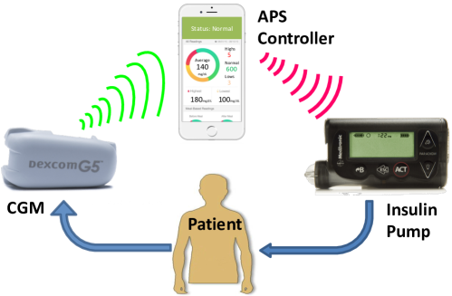
Figure 1: Artificial Pancreas System (APS).

2.1 Artificial Pancreas Systems

Our main case study in this paper is Artificial Pancreas Systems (APS), an autonomous medical CPS used for the treatment of Type I diabetes. The structure of a typical APS is shown in Fig. 1, including a continuous glucose monitor (CGM), an insulin pump, and a controller. At each control cycle, the APS controller estimates the current blood glucose (BG) level and insulin on board (IOB) based on measurements from the CGM sensor and decides on the dose of insulin to be injected through an insulin pump based on the patient’s treatment targets, physical activities, and other parameters. IOB represents the remaining insulin in the patient’s body, which will continue to digest blood glucose and should be considered for more accurate prediction of future BG trajectory as well as for the decision on insulin injections. Attacks or faults targeting any of the APS components, including the CGM, insulin pump, or the controller, can lead to underdose or overdose of insulin and risk of harm to patients [23, 1, 24]. As shown in Fig. 1, the modern APS controllers are implemented as mobile apps that communicate with the CGM and insulin pump wirelessly. Previous recalls and vulnerability reports have shown the possibility of the APS software and wireless link being compromised by attackers to threaten system security and patient safety (see Table I).

TABLE I: Simulated Attack Scenarios and Representative Real-world Vulnerabilities and Adverse Events Reported for APS.

Attack Approach	Attack Target	Attack Examples	FDA Recalls1	Reported Vulnerabilities 2
Stop the insulin delivery	Availability [25]	[1, 26, 27]	Z-1890-2017, Z-2471-2018	Insecure wireless communication [1, 24, 28], CVE[29] Lack of encryption or authorization [30, 31], CVE[32] Open source software [33, 34] Mobile/App based control [35, 36]
Stop refreshing state variables		[37, 38, 39, 40, 41]	Z-0929-2020
Change insulin delivery amount	Integrity [42]	[1, 43, 44, 45]	Z-1583-2020, Z-1105-05
Change controller input values		[46, 23, 47, 48]	Z-0043-06, Z-1034-2015

• Recall IDs are assigned by the U.S. FDA and can be searched for on https://www.accessdata.fda.gov/scripts/cdrh/cfdocs/cfres/res.cfm.

• Vulnerabilities are identified from the related works and by searching the national vulnerability database using relevant keywords (e.g., insulin pump) [49].

2.2 Control System Model

At each control cycle $t$, a CPS controller estimates the system’s current state $x_{t}=(x^{1}_{t},x^{2}_{t},...,x^{p}_{t})$ based on sensor measurements, decides a control action $u_{t}$ to change the state of the physical system based on the current state and control targets, and sends $u_{t}$ as a control command to the actuators. Upon execution of the $u_{t}$ by the actuators, the physical system will transition to a new state $x_{t+1}$.

We consider three typical regions of operation in the state space of a CPS controller. The unsafe/hazardous region ${\mathcal{X}}_{h}$ is defined as the set of states that lead to adverse events (e.g., the set of BG and IOB values corresponding to hyperglycemia and hypoglycemia events). The safe/target region ${\mathcal{X}}_{*}$ is defined based on the goals and guidelines of the specific application (e.g., keeping BG in the target range of 120-150 mg/dL). The set of states not included by either of these regions is referred to as the possibly hazardous region ${\mathcal{X}}_{*<h}$.

For modeling the multi-dimensional context in CPS (including physical processes and environment that affect the cyber processes) and the human-interpretable specification of their interactions in both temporal and spatial domains, we define $\mu(x_{t})=(\mu_{1}(x_{t}),\dots,\mu_{m}(x_{t}))\in\mathbb{R}^{m}$, where $\mu_{i}(x_{t})$ are transformations of $x_{t}$, (e.g., derivative, polynomial combinations, or other functions) modeling more complex combinations of state variables and their rates of change. The set of all possible values of $\mu(x_{t})$ is denoted by $\mathcal{M}$. We describe the system context $\rho(\mu(x_{t}))$ as subsets of $\mathcal{M}$, defined by ranges of variables in $\mu(x_{t})$, that can be mapped to the regions $\{{\mathcal{X}}_{*},{\mathcal{X}}_{*<h},{\mathcal{X}}_{h}\}$. To identify the nature of a control action $u_{t}$ within a context $\rho(\mu(x_{t}))$, we need to determine the possibility that by issuing $u_{t}$ the system eventually transitions into a new context $\rho(\mu(x_{t^{\prime}}))$ within the hazardous region ${\mathcal{X}}_{h}$. Fig. 2 shows example regions of operation for APS and a state trajectory where an attack on controller state variables causes the system’s transition into the unsafe region.

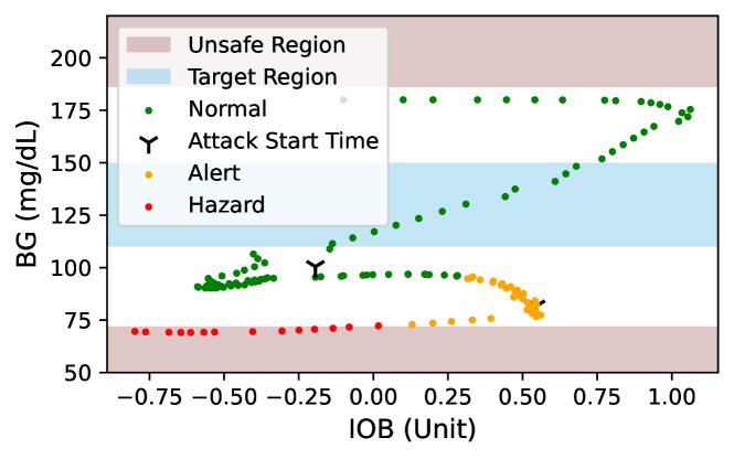
Figure 2: Example Regions of Operation and an APS System State Trajectory under Attack.

2.3 Threat Model

We focus on accidental faults or malicious attacks targeting the CPS controller that, if activated under certain triggering conditions, can manifest as errors in the inputs, outputs, or internal state variables of the control software and cause unsafe control actions and hazardous system states, which, together with a worst-case set of environmental conditions, could lead to adverse events [50], such as those reported in the literature or public datasets, e.g., severe complications from hypoglycemia or hypoglycemia [51, 52]. We assume such errors are transient and only occur once for a particular duration. We aim to mitigate these faults/attacks by predicting hazardous system states and correcting unsafe control actions.

The attackers can change the controller state through external or insider threats. For example, they can modify the values of the controller state variables by exploiting the known vulnerabilities in the communication channels of devices [53, 26, 32], underlying operating system (e.g., malicious wrappers for system libraries) [53], or control-semantic bugs (e.g., input validation bugs) [9]. The increasing popularity of open-source [54] and mobile app-based [35, 55] controllers and wireless/radio communications [56] further raises the possibility of such attacks. The attackers can also obtain unauthorized remote access to the control software by exploiting weaknesses such as stolen credentials [57], vulnerable services [58], and unencrypted communication [3]. Even for a control system that does not connect to a network, the attacker can still exploit USB ports or Bluetooth to get one-time access and deploy malware. Table I presents the simulated attack scenarios in this paper and representative real-world vulnerabilities and recalls reported to the U.S. Food and Drug Administration (FDA) for APS.

We assume that the attacks conceal their malicious behavior until the control software has received the sensor data and thus evade the anomaly detection on sensor measurements and threaten the controller’s safety. We also assume that the sensor measurements received by the safety engine and mitigation modules are not compromised since existing sensor anomaly detection approaches [11, 7, 8, 2, 20] can easily detect such sensor attacks and prevent their propagation into the safety engine. We assume that the safety engine is made tamper-proof (e.g., using protective memories or hardware isolation [59]) and is integrated with the CPS controller as a wrapper with only access to the input and output data without any changes to the original system architecture.

2.4 Design Challenges

As mentioned in the introduction, the existing works on enhancing APS security mainly focus on encryption [60], intrusion detection [61], safety specification [62], and model-based [63] or data-driven [6] run-time monitoring with less attention paid to hazard mitigation. The only work we found that attempts to avoid hazards in APS includes a fail-safe approach that shuts down the pump or stops insulin delivery under attack [12, 13]. However, this approach fails to maintain the regular operation of APS.

The major challenges impeding the effectiveness of existing mitigation and recovery methods include (C1) strict timing constraints for taking corrective actions and preventing adverse events, (C2) cyber-physical state explosion in reachability analysis and the generation of corrective control action sequences, and (C3) lack of realistic closed-loop testbeds for simulation of safety-critical fault/attack scenarios and testing the mitigation strategies without the risk of adverse consequences.

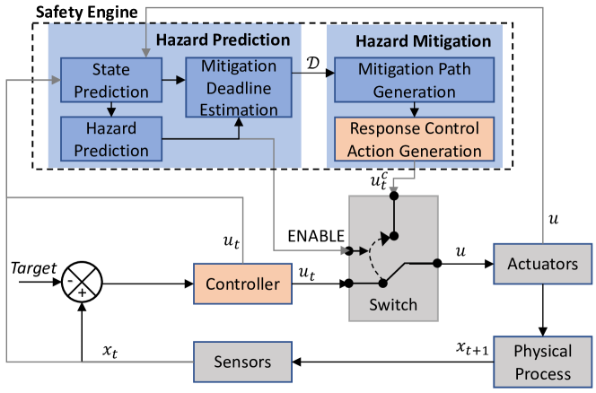
Figure 3: Combined Knowledge and Data Driven Safety Engine for Hazard Prediction and Mitigation.

3 Combined Knowledge and Data Driven Hazard Mitigation Approach

To overcome the aforementioned challenges, this paper proposes a combined knowledge and data driven approach for designing a safety engine that can predict and mitigate potential hazards at run-time. Fig. 3 shows the overall design of the safety engine, consisting of a hazard prediction module (Section 3.1) and a hazard mitigation module, with mitigation path planning (Section 3.2) and corrective control action generation (Section 3.3).

At each control cycle, the hazard prediction module takes as input a sequence of system states or their transformations as inferred from sensor data and precisely estimates their future trend and trajectory for hazard prediction (C1). The time between the current time and when the inferred hazard will happen is defined as the mitigation deadline or the budget to launch corrective or response control actions and mitigate hazards. If any potential hazards are inferred, the hazard mitigation module generates an optimal path and a corresponding control action sequence to keep the system away from the unsafe region and return it to the target region under the constraint of mitigation deadline and other domain-specific safety requirements (C2).

3.1 Reachability Analysis and Hazard Prediction

Anomaly detection is a critical step in hazard mitigation and recovery. Previous works on anomaly detection and recovery mainly focus on comparing the predicted states with actual states based on sensor data and waiting until a large deviation over a detection window to raise an alarm [11, 7]. However, relying on predefined thresholds for detecting deviations may lead to delayed detection and high false positive rates, resulting in mitigation failures. In this work, we propose a hazard prediction method that estimates the possible sequence of future system states and whether they will fall within any unsafe regions of operation.

Problem Statement: We specifically define the following binary classification problem:

$$y_{t}=\begin{cases}1,&\text{ if }\exists t^{\prime}\in[t,t+N]:\{\hat{x}_{t^{\prime}}\in g(X_{t},U_{t})\}\subset{\mathcal{X}}_{h}\\ 0,&\mathrm{otherwise}\end{cases}$$ (1)

where $g(\cdot)$ is a prediction model that given an input state sequence $X_{t}=\{x_{t-k},...,x_{t}\}$ and the control action sequence $U_{t}=\{u_{t-k},...,u_{t}\}$, predicts the system state trajectory $\hat{X}_{t+N}=\{\hat{x}_{t+1},...,\hat{x}_{t+N}\}$ within a prediction window of $N$ control cycles. A hazard is predicted to occur if any predicted state $\hat{x}_{t+i}$ is located within the unsafe region $\mathcal{X}_{h}$. The mitigation deadline, $\mathcal{D}$, is further estimated by calculating the difference between current time $t$ and the minimum $t^{\prime}$ within the prediction window such that the system state $\hat{x}_{t^{\prime}}$ is unsafe.

$$\mathcal{D}=min\{t^{\prime}\in[t,t+N]\}-t:\hat{x}_{t^{\prime}}\in\mathcal{X}_{h}$$ (2)

Domain Knowledge Specification: To ensure that the predicted system state sequences are accurate and realistic, we need to check a set of application-specific constraints, e.g., whether the change from the start state to the predicted states is within a reasonable range. These properties are often described in human-interpretable format over a transformed state space representing the derivatives, polynomial combinations, or other functions of state variables (e.g., the first derivative of blood glucose to represent the rate of change). So we project the current state $x_{t+i}$ and its prediction in the next step $\hat{x}_{t+i+1}$ to the transformed state space of $\mu(x)=(\mu_{1}(x),\mu_{2}(x),...,\mu_{m}(x))$. Then, we define the $\delta$ reachable state of $\mu(x_{t})$ as a set or region $\mathcal{S}(\mu(x_{t}),\delta)$, such that the difference between any states within this region $\mathcal{S}$ and the state $\mu(x_{t})$ is constrained by the parameter set $\delta$ as shown in Eq. 3:

$$\mathcal{S}(\mu(x_{t}),\delta):=\{\forall s_{t}\in\mathcal{S},|s_{t}-\mu(x_{t})|\leq\delta\}$$ (3)

where $\delta=(\delta_{1},\delta_{2},...,\delta_{m})$ is a set of parameters for each variable in $\mu(x)$ and could be derived based on domain-specific guidelines, design requirements, practical experience, or statistical analysis of the past data.

Data and Knowledge Integration: In this paper, we develop a novel multivariate regression neural network model (referred to as PredNet) to predict the sequence of system states using either the data collected from closed-loop CPS simulations or real system operation (e.g., from clinical trials as described in Section 4.5). As shown in Fig. 4, our prediction network is based on an encoder-decoder model that predicts the future system states $x_{[t+1:t+N]}$ for $N=n$ steps based on a sequence of $k+1$ past system states.

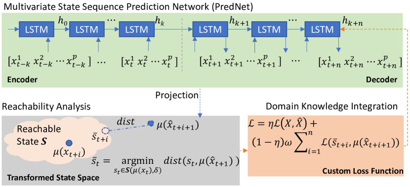
Figure 4: Multivariate Regression Neural Net for Sequential States Prediction (PredNet) with Domain Knowledge Integration.

The domain-specific properties are integrated with PredNet by adding a customized loss function as the regularization term to the original loss function $\mathcal{L}(X,\hat{X})$ (e.g., mean squared error), as shown below:

$$\mathcal{L}=\eta\mathcal{L}(X,\hat{X})+(1-\eta)\omega\sum_{i=1}^{n}\mathcal{L}(\bar{s}_{t+i},\mu(\hat{x}_{t+i+1}))$$ (4)

$$\bar{s}_{t}=\underset{s_{t}\in\mathcal{S}(\mu(x_{t}),\delta)}{\mathrm{argmin}}dist(s_{t},\mu(\hat{x}_{t+1}))$$ (5)

where, $\bar{s}_{t+i}$ is the state within the $\delta$ reachable state of $\mu({x}_{t+i})$ that has the minimum distance (e.g., Euclidean distance) to the predicted state transformation $\mu(\hat{x}_{t+i+1})$, and $\omega$ is a weight parameter that takes a zero value when $\mu(\hat{x}_{t+i+1})$ is within the reachable state $S$ and a unit value otherwise. $\eta\in[0,1]$ represents the weight of original loss contributing to the total loss. In this paper, we select the value of $\eta$ by manual hyper-parameter tuning. The custom loss function enforces realistic trajectories by penalizing PredNet during training whenever a predicted state is outside the reachable set of the current state.

We also design a two-level hazard prediction pipeline consisting of (i) a long-term prediction model (PredNet-l) that can predict a far-future state sequence with the benefit of ensuring enough time to foresee and mitigate potential hazards, and (ii) a short-term prediction model (PredNet-s) that has higher accuracy than the long-term model, ensuring we do not miss any hazards.

3.2 Mitigation Path Generation

The next major step in hazard mitigation is the selection of response actions that the system should take to complete its mission (i.e., end up or stay within the target region for the controller) safely. A simple algorithm to execute the proposed mitigation might involve control action compensation based on fixed rules or medical guidelines (e.g., increase insulin injection to prevent hyperglycemia in APS). However, such a generic mitigation mechanism does not consider the current context of the system or its interactions with the environment and might lead to over-/under-mitigation or potential harm to system users [6]. It is challenging to design a mitigation mechanism with a high recovery rate that introduces as few new hazards as possible.

Our goal is to learn a sequence of control actions that can mitigate hazards and keep the system away from unsafe regions. Simply, we could feed all the possible actions to the prediction model introduced above and select the optimal one that results in a future system state sequence closest to the safe region. However, this approach would be time- and resource-consuming as we must traverse the whole action space and may not converge to an optimal solution within the required mitigation deadline. Therefore, instead of generating the recovery control actions directly, we first find the desired sequence of recovery states (using a fast path planning algorithm) and then use a control algorithm (ML-based or model-based) to generate a corresponding sequence of control actions.

Problem Statement: We model the mitigation path generation as an optimization problem with the goal of returning the system to the safe region as fast as possible and before the occurrence of hazards while avoiding the unsafe region. Specifically, we minimize the time to mitigate the hazard under the constraints shown in the following equations:

min $$\{TimetoMitigation\};\ \text{s.t.}\$$ (6)

$${\Delta x_{i}}/{T}<{\alpha}_{i}^{1};\forall i\in[1,p]$$ (7)

$${\Delta(\Delta x_{i})}/{T^{2}}<{\alpha}_{i}^{2};\forall i\in[1,p]$$ (8)

$$\{x\}\cap\mathcal{X}_{h}=\varnothing$$ (9)

$$PathLength<\mathcal{D}\vspace{-2em}$$ (10)

where, $x$ is the system state, $T$ is the duration of a control cycle, and $\alpha_{i}^{j}$ is an application-specific constraint. $\mathcal{D}$ is the maximum mitigation budget to mitigate hazards and the maximum length of mitigation path ($PathLength$), estimated using the hazard prediction module (see Fig. 3).

Domain Knowledge Specification: The constraints ${\alpha^{j}_{i}}$ ensure satisfying the safety proprieties and keeping the smoothness between state transitions and are specified based on domain knowledge or practical experience. For example, the change of BG in APS should not exceed [-5,3] $mg/dL$ per 5 minutes [6].

Data and Knowledge Integration: We develop a mitigation path planning algorithm with the knowledge of safety constraints (referred to as SC-RRT*) based on a variant of a path planning algorithm called Rapidly-exploring Random Tree Star (RRT*) [64], which can easily handle problems with obstacles and differential constraints with a wide search range, fast search speed, and high computational efficiency and has been widely used in robotic motion planning. SC-RRT* is a lightweight algorithm with more transparency than neural networks and more suitable for implementation on devices with limited memory and computation resources.

Algorithm 1 shows the overall mitigation path generation process. At each exploration cycle, the algorithm randomly samples a point in the state space (line 17) and configures a new vertex in the random tree $G$ in the direction from the nearest vertex not exceeding the incremental distance $\Delta x$ (lines 18-19). We encode the domain knowledge as safety constraints to filter out the invalid vertices in the random sampling step. Specifically, a random-sampled vertex is only added to the tree if its connection to the nearest node satisfies the safety requirements defined in Eq. 7-10. The edges between the new node and its neighbor nodes within a radius $\gamma$ are further updated if any lower-cost connects are found (lines 22-27). A mitigation path is found if the destination locates inside the target region $\mathcal{X}_{*}$ (lines 28-29). Finally, an optimal destination vertex and mitigation path are selected (line 31) with the shortest path from the current state to the target state while optimizing other application-specific requirements (e.g., maximizing the smoothness or minimum distance to $\mathcal{X}_{h}$).

1

Input: Initial config $x_{init}$, Number of vertices $K$, Incremental distance $\Delta$x, Near Radius $\gamma$, Recovery Budget $D$

2

Output: RRT graph G, Optimal Goal Vertex $x_{optimal}$ , Minimum recovery path $path_{min}$

3 G.init($x_{init}$) $\triangleright$ Init Optimal RRT

4 $X_{dest}$ $\leftarrow$ $\emptyset$ $\triangleright$ Vertices in Target Region

5

6 Function UpdateCost($X_{near}$, $x_{new}$):

7       for $x_{near}\in X_{near}$ do

8             if ValidConnection($x_{near},x_{new}$) then

9                   if Cost($x_{near}$)+Dist($x_{nearest},x_{new}$) < $cost_{min}$ then

10                         $x_{min}\leftarrow x_{near},cost_{min}$ $\leftarrow$

11                         Cost$(x_{near})$+Dist($x_{nearest},x_{new}$)

12                        

13                  

14            

15       end for

16      

17

18return

19 Function RewriteTree($X_{near}$, $x_{new}$):

20       for $x_{near}\in X_{near}$ do

21            

22            G.update($G,x_{near},x_{new}$) $\triangleright$ update shorter path with $x_{new}$

23       end for

24      

25

26return

27for k = 1 to K do

28       $x_{rand}$ $\leftarrow$ RandomSampling()

29       $x_{nearest}$ $\leftarrow$ FindNearestNode(G,$x_{rand}$)

30       $x_{new}$ $\leftarrow$ NewConf($x_{nearest}$, $x_{rand}$, $\Delta$ x)

31      

32      if ValidConnection($x_{nearest}$,$x_{new}$) then

33             $G.add\_node(x_{new})$

34             $X_{near}\leftarrow$ FindNearNodes(G,$x_{new}$,$\gamma$)

35             $x_{min}\leftarrow x_{nearest}$

36             $cost_{min}\leftarrow$ Cost($x_{nearest}$)+Dist($x_{nearest},x_{new}$)

37            

38            UpdateCost($X_{near}$, $x_{new}$)

39            

40            G.add_edge($x_{min},x_{new}$) $\triangleright$ Shortest path to $x_{new}$

41             RewriteTree($X_{near}$, $x_{new}$)

42      

43      if $x_{new}$ $\in$ Goal then

44             $X_{dest}\leftarrow X_{dest}\cup x_{new}$

45      

46 end for

47$x_{optimal},path_{min}\leftarrow$ FindOptimalNode($G,\mathcal{X}_{*}$)

return G, $x_{optimal}$, $path_{min}$

Algorithm 1 Mitigation Path Planing Algorithm

3.3 Response Control Action Generation

Once the target state trajectory is generated, it can be fed to a control algorithm (either ML-based or model-based) to generate the final sequence of corrective/recovery control actions that realize the desired state trajectory.

Problem Statement: We model the task of generating a sequence of control actions as a context-specific multivariate sequence-to-sequence regression problem, as shown below:

$$y_{t}=f(\bar{X}_{t+n})=\hat{U}_{t+n-1},\text{s.t.}$$ (11)

$$\forall t^{\prime}\in[t,t+n-1]:x_{t^{\prime}}\overset{u_{t^{\prime}}}{\rightarrow}x_{t^{\prime}+1}$$

Given the expected system state sequence ${\bar{X}}_{t+n}=\{\bar{x}_{t+1},...,\bar{x}_{t+n}\}$, the controller outputs a control action sequence $\hat{U}_{t+n-1}$ = $\{\hat{u}_{t}$, $...$, $\hat{u}_{t+n-1}\}$ that if executed sequentially by the actuators should transition the system to the expected states.

Domain Knowledge Specification: The goal of mitigation is that given the current system context and prediction of a potential hazard, a new corrective control action $u^{c}_{t}$ from a set of control actions $\boldsymbol{u}^{\rho}$ is sent to the actuators to force the system transition into the target or safe region. The context-specific corrective control actions could be specified based on domain knowledge. Here, we use a formal framework based on Signal Temporal Logic (STL) for the human-interpretable description of the mitigation actions. STL is a formal specification and machine-checkable language often used for rigorous specification and run-time verification of requirements with time constraints in CPS [65]. For the system context $(\rho(\mu(x_{t}))$, we describe the Hazard Mitigation Specification (HMS) $(\rho(\mu(x_{t})),u^{c}_{t})\mapsto{\mathcal{X}}_{*}$ as follows:

where $F$ is the eventually operator requiring that $u^{c}_{t}\in\boldsymbol{u}^{\rho}$ should be taken within period $t_{s}$ since (denoted by the $S$ operator) the system enters context $\rho(\mu(x_{t}))$ measured by $(\varphi_{1}(\mu_{1}(x_{t}))\land\ldots\land\varphi_{m}(\mu_{m}(x_{t})))$. Each $\varphi_{i}(\mu_{i}(x_{t}))$ is an atomic predicate that represents an inequality on $\mu_{i}(x_{t})$ in the form of $\mu_{i}(x_{t})\{<,\leq,>,\geq\}{\beta}_{i}$ or its combinations, where the inequality thresholds ${\beta}_{i}$ define the boundary of the subset in that dimension $\rho(\mu_{i}(x_{t}))$. This should hold globally (denoted by the $G$ operator) between the start time $t_{0}$ and the end time $t_{e}$ of the system operation. The time parameter $t_{s}$ specifies the requirement for the latest possible time a mitigation action should be initiated after a potential unsafe control action is detected to prevent hazards. The estimated time between the activation of a fault/attack on the system and the occurrence of a hazard can provide an upper bound for specifying this time requirement.

The formal safety specifications are usually generated by safety analysts in cooperation with domain experts using hazard analysis approaches [6, 66]. In this paper, we adopt a control-theoretic hazard analysis method (called STPA [50]) to generate HMS by following these steps:

1. Define the hazards and adverse events of interest.

2. Identify the observable set of variables $x_{t}$ of interest related to the hazards and decide on the possible transformations $\mu(x_{t})$ and the sets $\rho(\mu(x_{t}))$ as completely as possible.

3. List all the combinations of $\rho(\mu(x_{t}))$ and control action $u_{t}$ and identify the combinations that might result in transitions to a hazardous region ${\mathcal{X}}_{h}$. The unknown boundaries $\beta_{i}$ can be learned from a population dataset using off-the-shelf optimizers (e.g., Newton’s method) [6, 66].

4. For each unsafe context in step 3, find all control actions $u^{c}_{t}\in U$ such that $(\rho(\mu(x_{t})),u^{c}_{t})\mapsto{\mathcal{X}}_{*}$ and add these tuples $(\rho(\mu(x_{t})),u^{c}_{t})$ to HMS for that context.

5. Formalize the generated HMS into STL format.

An example of generated STL hazard mitigation specification for APS is shown in Table II, where a set of STL rules are specified to mitigate potential hazards that may result in hyperglycemia or hypoglycemia events. For example, the first rule states that since the system context that BG is larger than the target and keeps increasing and IOB is less than a threshold $\beta_{1}$ and keeps decreasing, an increase_insulin action $u_{2}$ should be issued by the controller within time $t_{s}$ to avoid hyperglycemia event. This safety property should be held true during the whole operation period.

TABLE II: STL Hazard Mitigation Specifications for APS.

Rule	Mitigation Action	STL Description of Safety Context
1	${G_{[t_{0},t_{e}]}((F_{[0,t_{s}]}(u_{2}))}$	$\mathcal{S}((BG>BGT\wedge BG^{\prime}>0)\wedge(IOB^{\prime}<0\wedge IOB<\beta_{1})))$
2	${G_{[t_{0},t_{e}]}((F_{[0,t_{s}]}(u_{2}||u_{4}))}$	$\mathcal{S}((BG>BGT\wedge BG^{\prime}>0)\wedge(IOB^{\prime}=0\wedge IOB<\beta_{2})))$
3	${G_{[t_{0},t_{e}]}((F_{[0,t_{s}]}(u_{2}||u_{4}))}$	$\mathcal{S}((BG>BGT\wedge BG^{\prime}<0)\wedge(IOB^{\prime}>0\wedge IOB<\beta_{3})))$
4	${G_{[t_{0},t_{e}]}((F_{[0,t_{s}]}(u_{2}||u_{4}))}$	$\mathcal{S}((BG>BGT\wedge BG^{\prime}<0)\wedge(IOB^{\prime}<0\wedge IOB<\beta_{4})))$
5	${G_{[t_{0},t_{e}]}((F_{[0,t_{s}]}(u_{2}||u_{4}))}$	$\mathcal{S}((BG>BGT\wedge BG^{\prime}<0)\wedge(IOB^{\prime}=0\wedge IOB<\beta_{5})))$
6	${G_{[t_{0},t_{e}]}((F_{[0,t_{s}]}(u_{3}))}$	$\mathcal{S}((BG<BGT\wedge BG^{\prime}<0)\wedge(IOB^{\prime}>0\wedge IOB>\beta_{6})))$
7	${G_{[t_{0},t_{e}]}((F_{[0,t_{s}]}(u_{1}||u_{3}))}$	$\mathcal{S}((BG<BGT\wedge BG^{\prime}<0)\wedge(IOB^{\prime}<0\wedge IOB>\beta_{7})))$
8	${G_{[t_{0},t_{e}]}((F_{[0,t_{s}]}(u_{1}||u_{3}))}$	$\mathcal{S}((BG<BGT\wedge BG^{\prime}<0)\wedge(IOB^{\prime}=0\wedge IOB>\beta_{8})))$
9	${G_{[t_{0},t_{e}]}((F_{[0,t_{s}]}(\neg u_{3}))}$	$\mathcal{S}((BG>BGT\wedge IOB<\beta_{9})))$
10	${G_{[t_{0},t_{e}]}((F_{[0,t_{s}]}(u_{3}))}$	$\mathcal{S}((BG<\beta_{10})))$

• BGT: BG target value, IOB: Insulin on board; $BG^{\prime}=dBG/dt$, $IOB^{\prime}=dIOB/dt$;

• $u_{1,2,3,4}:$decrease_insulin, increase_insulin, stop_insulin, keep_insulin;

It should be noted that there is a semantic gap between the high-level human-interpretable state variables $\mu(x)$ in the HMS (e.g., rate of BG change) and the sensor measurements (e.g., BG values from CGM) as well as the high-level control actions $u_{t}^{c}$ (e.g., increase insulin) and the low-level control commands sent to the actuator (e.g., the amount of insulin dose). To close this gap during actual implementation, an additional step is needed to infer the values of state variables in the transformed state space based on the sensor measurements (e.g., by taking the derivative of BG values to calculate the rate of BG change) and the high-level control commands based on the ML predictions, using the transformation function $h(\cdot)$ (see Eq. 13). These transformations enable matching of the estimated states and control actions with the logic formulas specified in HMS to check the satisfaction of any of the safety properties (e.g., Rules 1-5 in Table II will be checked for control action $u_{2}$).

Data and Knowledge Integration: In this paper, we integrate the domain-specific knowledge on context-dependent mitigation actions with state variable and control output data traces collected from closed-loop CPS simulation or real operation to train an RNN for control action generation (referred to as ActNet). We encode the logic formulas generated for HMS as a custom loss function that penalizes the RNN model during the training process if the ML prediction does not match the specified mitigation action properties:

$$\vspace{-0.25em}\mathcal{L}=\eta\mathcal{L}(U,\hat{U})+(1-\eta)k(2\sigma(\sum_{h(y_{t})\notin u_{t}^{c}}\omega_{i})-1)$$ (13)

where, $h(\cdot)$ is a transformation function (e.g., derivation) that transfers the predicted control command $y_{t}$ to a discrete high-level control action as described above, and $w$ is a weight parameter that defines the impact of each logic rule on the training process. $\sigma(\cdot)$ is a sigmoid function that maps the degree of satisfaction of the ML outputs with the STL formulas to the range of [0,1], and $k$ is a scaling factor that scales the sigmoid function to a similar range with the original loss $\mathcal{L}(U,\hat{U})$ (e.g., mean squared error).

3.4 Safety Engine Implementation

1

2 Function Mitigation():

3       if $MitEnable$  then

4             if $x_{t}\in\mathcal{X}_{*}$ or $kMit\geq\mathcal{D}$ then

5                   $MitEnable\leftarrow False$ $\triangleright$ Stop

6                   $kMit\leftarrow 0$

7                   if $x_{t}\notin\mathcal{X}_{*}$ then

8                         RaiseAlert("Mit. Failure!")

9                        

10                  

11            else

12                   if $kMit>0$ and $err({\bar{X}}_{[kMit-1]},x_{t})>\theta$ then

13                        

14                        ${\bar{X}}\leftarrow SC\_RRT^{*}(x_{t},\mathcal{D}-kMit,QuickMit)$

15                         $U^{c}\leftarrow ActNet({\bar{X}})$ $\triangleright$ Update

16                         $kMit\leftarrow 0$

17                         $\mathcal{D}\leftarrow\mathcal{D}-kMit$

18                        

19                  

20                  $u\leftarrow GetAction(U^{c},kMit)$ $\triangleright$ Replace

21                  

22                  $kMit\leftarrow kMit+1$

23                  

24             end if

25            

26      else

27             $u\leftarrow u_{t}$

28            

29       end if

30      Actuate($u$)

31

32return

33$x\leftarrow$ System State

34 $u\leftarrow$ Control Action to the Actuator

35 $Hazard\leftarrow False$ $\triangleright$ Hazard Prediction Flag

36for each control cycle t do

37       $X_{t}\leftarrow UpdateState(x_{t})$

38       $U_{t}\leftarrow UpdateAction(u_{t})$ $\triangleright$ Original Control Action

39      

40      if MitEnable==False then

41             $kMit\leftarrow 0$

42             $\hat{x}_{[t+1:s]}\leftarrow PredNet\textit{-}s(X_{t},U_{t},s)$ $\triangleright$ Short-term

43             if $\{\hat{x}_{[t+1:s]}\}\cap\mathcal{X}_{h}$ then

44                   $MitEnable\leftarrow True$

45                   $\mathcal{D}\leftarrow Deadline(\hat{x}_{[t+1:s]})$

46                   $QuickMit\leftarrow True$

47                  

48             else

49                   $\hat{x}_{[t+1:l]}\leftarrow PredNet\textit{-}l(X_{t},U_{t},l)$ $\triangleright$ Long-term

50                  

51                  if $\{(\hat{x}_{[t+1:l]}\}\cap\mathcal{X}_{h}$ then

52                         $MitEnable\leftarrow True$

53                         $\mathcal{D}\leftarrow Deadline(\hat{x}_{[t+1:l]})$

54                        

55                        $QuickMit\leftarrow False$

56                        

57                  

58             end if

59            if MitEnable  then

60                   ${\bar{X}}\leftarrow SC\_RRT^{*}(x_{t},\mathcal{D},QuickMit)$

61                   if $\bar{X}==\emptyset$ then

62                         RaiseAlert("Mit. Path Not Found!")

63                         break

64                   $U^{c}\leftarrow ActNet({\bar{X}})$ $\triangleright$ Corrective Action Seq.

65                  

66            

67       end if

68      

69      Mitigation()

70 end for

Algorithm 2 Hazard Prediction and Mitigation

The overall hazard prediction and mitigation procedure is shown in Algorithm 2. Our two-level hazard prediction framework consists of (i) a long-term prediction model (PredNet-l) that can predict a far-future state sequence with the benefit of ensuring enough time to foresee and mitigate potential hazards (line 36), and (ii) a short-term prediction model (PredNet-s) with higher accuracy than the long-term model, ensuring we do not miss any hazards (line 30). The control system will raise an alert and switch to the Mitigation mode when any predicted system state sequence overlaps the unsafe region $\mathcal{X}_{h}$ (lines 31-32 and lines 37-38). To reduce computation time (see Section 4.10), PredNet-l is executed only when PredNet-s does not infer a hazard in a near future.

An optimal mitigation path is generated based on the remaining mitigation budget (line 43). Strict constraints are used to generate the mitigation path if the potential hazards are captured by the long-term hazard prediction model (with a larger mitigation budget), which satisfies the smoothness and safety constraints during the mitigation process (lines 36-40). In contrast, if a hazard is not predicted by the long-term model but by the short-term model, loose constraints (e.g., wider ranges of $\alpha^{j}_{i}$ in Eq. 8) will be applied to ensure fast mitigation within the short mitigation deadline (lines 31-34). These prediction models and mitigation path generation strategies compensate for each other to improve the mitigation performance. Then a sequence of corrective control actions $U^{c}$ is derived by feeding the mitigation path to the mitigation action generation model (ActNet) (line 47).

When running in the Mitigation mode (line 2), the $GetAction$ function sequentially selects a mitigation action $u^{c}_{kMit}$ from the set $U^{c}$ (line 14), which will be then sent to be executed by the actuators (line 20). To make a trade-off between accuracy and computation overhead, the mitigation path and control action sequences are only updated when the error between the actual state $x_{t}$ and the expected state in the mitigation path $\bar{X}$ exceeds a preset threshold $\theta$ (line 9). The Mitigation mode remains active until the system returns to the target region $\mathcal{X}_{*}$ or the mitigation budget $\mathcal{D}$ has been used up (lines 3-5). The user (patient) or physician will be warned of any mitigation failures (e.g., no safe path is found (line 45), or the budget is used up without reaching a safe state (line 7)).

4 Experimental Evaluation

To overcome the last design challenge (C3) mentioned in Section 2.4, we develop an open-source simulation environment (see Fig. 5) that integrates the closed-loop simulation of two example APS controllers with an adverse event simulator to evaluate different safety engines. We run the experiments with both APS controllers and simulators on an x86_64 PC with an Intel Core i9 CPU @ 3.50GHz and 32GB RAM running Linux Ubuntu 20.04 LTS. We use TensorFlow v.2.5.0 to train our ML models and Scikit-learn v.1.1.1 for data pre-processing and experimental evaluation.

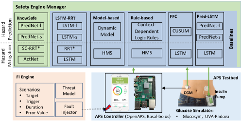
Figure 5: Experimental Platform with different Safety Engines, integrated with an APS controller running on a PC/cellphone or an embedded device (e.g., Raspberry Pi 4), a Glucose Simulator, and a Software Fault Injection Engine

4.1 Experimental Platform

As shown in Fig. 5, the APS testbed integrates two widely-used APS controllers (OpenAPS [34] and Basal-Bolus [67]) with two different patient glucose simulators, including Glucosym [68] and UVA-Padova Type 1 Diabetes Simulator [69]. The Glucosym simulator contains models of 10 actual Type I diabetes patients aged 42.5 $\pm$ 11.5 years [70]. The state-of-the-art UVA-Padova Type 1 Diabetes Simulator contains 30 virtual patients, which were demonstrated to be representative of the Type 1 diabetes mellitus (T1DM) population observed in a clinical trial [71], and has been approved by the FDA for pre-clinical testing of APS [69]. This closed-loop testbed was also validated using actual data from a clinical trial, and the simulated data was shown to satisfy the requirements of relevance, completeness, accuracy, and balance [72] for developing ML models [5].

In each experiment, the patient simulator interacts with the APS controller for 150 iterations (about 12.5 actual hours), with each step/iteration in the simulation representing 5 minutes in the real APS control system. Simulations begin with the patient at different initial glucose values within the normal range of 70 to 180 $mg/dL$ without additional meals or exercise during the simulation period, mimicking a scenario of the patient at nighttime after eating dinner. To account for inter-patient variability, each system version (without a safety engine and with each different safety engine) is evaluated using ten patient profiles in each glucose simulator.

4.2 Adverse Event Simulation

We run the closed-loop simulation of a glucose simulator and an APS controller with a source-level fault injection (FI) engine that directly perturbs the values of the controller’s state variables within their acceptable ranges over a random period to simulate the effect of accidental faults or attack scenarios introduced in Section 2.3 (Table I). We simulate two categories of attacks:

• Availability attacks set the control output to zero (Min scenario for the Rate variable in Table III) or keep the same sensor measurements after the ${k}_{th}$ control cycle for m steps $x_{k:k+m}=x_{k}$ (Hold scenario in Table III).

• Integrity attacks add a bias $b$ to the sensor readings $x_{k}=x_{k}+b$ (Add, Subtract, Max, and Min scenarios in Table III).

TABLE III: Adverse Event Simulation Experiments Per Patient.

Target State Variables	Scenario	Attack Value		No. Simulations
		BG	Rate
Blood Glucose (BG)/ Insulin Output (Rate)	Hold	Repeat		63
	Add	[32,64]	[0.5,1]	126
	Subtract	[32,64]	[0.5,1]	126
	Max	175	2	63
	Min	80	0	63

For each FI scenario, the FI engine determines (i) the target state variable, (ii) the trigger condition for activating the fault, (iii) the duration of the fault, and (iv) the error values to be injected. In this paper, we utilize a random strategy that randomly chooses from several different start times and durations uniformly distributed within the entire simulation period to inject the faults, resulting in 882 FI simulations for each patient (3 start times $\times$ 3 durations $\times$ 7 initial BG values $\times$ 14 attack values, see the last column of Table III) and 17,640 simulations for all 20 patients in both simulators. This translates into 25.52 years of simulation data (17,640 $\times$ 12.5 hours) used for training and testing different safety engines. The details of each FI scenario are shown in Table III.

4.3 Adversarial Training

We use both normal and hazardous data for training hazard prediction models to improve robustness. For evaluation of the trained state and hazard prediction models, we consider the whole simulation trace as a sample and label it as hazardous if any state sequence in that simulation trace overlaps the unsafe region (e.g., BG value higher than 180 mg/dL or less than 70 mg/dL). For the training and testing of response control action generation models, we use a sequence of collected control actions $u_{t:t+n}$ as the ground truth values. The input to the models is the sequence of expected or target system states $x_{t+1:t+n}$ upon sequential execution of the control actions.

Our FI engine results in a total number of 3,230 (38.3%) simulations with hazards in the Glucosym simulator and 3,315 (37.6%) simulations with hazards in the UVA-Padova simulator, which are used for training and testing each ML model for hazard prediction and mitigation. We use a 4-fold cross-validation setup for training and testing each patient-specific ML model. Specifically, for each patient, we train separate ML models for state prediction and mitigation action generation using data from 75% of the simulation traces and test the models on the remaining 25% simulation traces.

To reduce the model complexity and computational resources, we minimize the number of layers of the neural network. We explored different model architectures, and the best model we obtained was a two-layer (128-64 units) stacked LSTM.

4.4 Metrics

We introduce the following metrics to evaluate the performance of the proposed methodology.

• Prediction Accuracy is measured using the root mean squared error (RMSE) between the predicted/generated trajectories and the ground truth trajectories. We also utilize the standard binary metrics of false positive rate (FPR), false negative rate (FNR), and F1 score to evaluate the accuracy of hazard prediction and mitigation action activation. We consider the whole trajectory of each simulation as a sample for evaluating performance.

• Reaction Time measures the timeliness of hazard prediction and indicates the maximum time budget to mitigate and prevent potential hazards. It is the time difference between when the prediction network detects the hazard and when the system enters a hazardous state.

• Mitigation Path Planning Efficiency is measured by evaluating the performance of each algorithm in finding an optimal mitigation path using the following two metrics:

  • Convergence Rate is the percentage of simulations in which a mitigation path ends up in a final state in the safe region.

  • Satisfaction Rate is the percentage of simulations with a valid mitigation path that satisfies safety constraints.

• Mitigation Outcome metrics evaluate the overall performance of the safety engine (the hazard prediction and mitigation pipeline):

  • Mitigation Success Rate (MSR) is calculated as the percentage of hazardous simulations in which the system transitions into the unsafe region without mitigation but after implementing the mitigation actions returns to the target region.

  • Out-of-Safe-Range Rate is the percentage of simulations with state variable values falling outside of the safe range (e.g., higher than 180 mg/dL or less than 70 mg/dL in APS). This metric measures the remaining hazard rate even with the mitigation algorithm, the summation of which is the complementary set of the Mitigation Success Rate.

  • Max Deviation measures the maximum distance from the safe region boundaries. This metric evaluates the risk of transitioning to an unsafe state with or without safety engine.

  • New Hazard Rate represents the percentage of non-hazardous simulations in which new hazards are introduced due to false alarms and performing unnecessary mitigation.

The final results are reported by calculating the average value of each metric over all cross-validation folds across all patients.

4.5 Prediction Accuracy

Table IV presents the performance of the proposed prediction models (PredNet) for system state and hazard prediction as well as mitigation deadline estimation in both glucose simulators compared to the baseline long short-term memory (LSTM) models that share the same architecture with the PredNet. We use "l" and "s" to differentiate the ML models with long-term and short-term prediction windows (e.g., 24 and 6 control cycles in this paper), respectively. The final results are reported by calculating the average value of each metric over all cross-validation folds across all patients.

With simulation data from Glucosym, we see that ML models trained under the guidance of domain knowledge achieve the best prediction accuracy with up to 37.7% lower root mean squared error (RMSE) (0.38 vs. 0.61) in state prediction and 28.1% lower RMSE (0.64 vs. 0.89) in deadline estimation. Although the PredNets only has slightly better F1 scores in hazard prediction (1.5%-3.8% improvement), they achieve zero false negative rates (FNR), which is important for hazard prediction and mitigation, while keeping false positive rate (FPR) up to 82.3% (0.003 vs. 0.017) lower. (The above binary metrics are evaluated by considering the whole trajectory of each simulation as a sample.)

TABLE IV: Performance of Each ML Model in Predicting System States and Estimating Deadlines of Mitigation Averaged over 8,820 Simulations in Glucosym and UVA-Padova Simulators, respectively. RMSE is measured in $mg/dL$ for state estimation and Iteration (representing 5 minutes in actual APS) for deadline estimation.

Simulator	Model	State	Hazard Prediction			Deadline
		RMSE	FNR	FPR	F1	RMSE
Glucosym	LSTM-l	2.34	0.037	0.091	0.909	0.89
	LSTM-s	0.61	0.008	0.017	0.982	0.17
	PredNet-l	1.46	0.014	0.061	0.943	0.64
	PredNet-s	0.38	0	0.003	0.997	0.13
UVA-Padova	LSTM-l	7.66	0.213	0.091	0.899	2.24
	LSTM-s	3.14	0.045	0.082	0.951	0.21
	PredNet-l	7.20	0.015	0.039	0.961	2.07
	PredNet-s	2.85	0	0.012	0.993	0.20

For tests in the UVA-Padova simulator, we observe similar performance improvements of combined knowledge and data driven ML models in hazard prediction (4.4%-6.9%) and system state prediction and deadline estimation, indicating the advantage of combining knowledge with data-driven approaches in predicting hazards and stable performance across different simulators and patients. However, the overall prediction error is higher in the UVA-Padova simulator than in the Glucosym simulator for all the models. This might be because the UVA-Padova simulator also includes a noise model for sensor measurement [73].

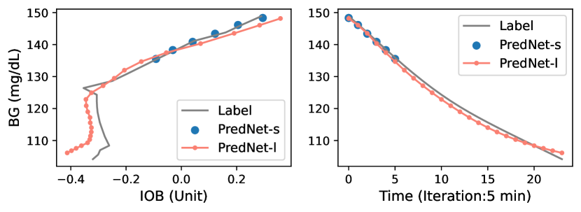
Figure 6: Example State Trajectories Predicted by Both Long-term and Short-term Hazard Prediction Models.

In Table IV, we also observe PredNet-s achieve up to 74.0% (0.38 vs. 1.46) and 90.3% (0.20 vs. 2.07) reduction of RMSE in state and deadline prediction, respectively, compared to PredNet-l, with at least 69.2% lower FPR (0.012 vs. 0.039) in predicting the occurrence of hazards while keeping a zero negative rate. This further attests to the benefit of employing two-level hazard prediction models, leveraging both the high accuracy of PredNet-s models to not miss any positive cases and the extended prediction window of PredNet-l models to preemptively mitigate potential hazards effectively. An example of the state trajectory and the predictions of PredNets is also shown in Fig. 6. As we can see, the PredNet-s predictions almost overlap with the ground-truth state trajectory, and the long-term predictions by PredNet-l also approximate the ground truth well.

To further evaluate the performance of the PredNet in actual APS and reduce the sim-to-real gap, we also train and evaluate the combined knowledge and data driven ML models for system state sequence prediction on a publicly available clinical trial dataset, PSO3 [22]. Experimental results show that our PredNet can achieve a slightly smaller RMSE than the ML models developed in a previous work (6.349 vs. 7.187 $mg/dL$ on average across the same patient data) [74]. We do not evaluate the hazard mitigation approach on actual APS as it requires run-time execution in a closed-loop system which would be safety-critical with actual patients.

4.6 Evaluation of Mitigation Path Generation

Table V presents the results of the mitigation path generation algorithm, SC-RRT*, in comparison with a baseline RRT* algorithm that does not consider application-based constraints (shown in Eq. 7-8 and the example in Table VI).

TABLE V: Performance of Each Mitigation Path Generation Algorithm (Averaged over All the Simulations). A unit of prediction length or path length represents 5 minutes in actual APS. Conv. Trials represents the number of trials each RRT algorithm takes to converge to a valid path.

Simulator	Prediction Model	Algorithm	Conv. Trials	Path Len	Satisfaction Rate
Glucosym	PredNet-s	SC-RRT*	174	15	89.4%
		RRT*	32	10	6.4%
	PredNet-l	SC-RRT*	194	25	85.8%
		RRT*	41	14	3.4%
UVA-Padova	PredNet-s	SC-RRT*	245	10	93.5%
		RRT*	78	8	31.9%
	PredNet-l	SC-RRT*	167	22	94.7%
		RRT*	50	17	32.0%

TABLE VI: Domain-Specific Constraints for APS. (BG is in mg/dL and IOB is in unit).

No.	Description	Constraint	No.	Description	Constraint
1	$dBG/dt$	[-5, 3]	3	$dIOB/dt$	[-0.1, 0.1]
2	$d^{2}BG/dt^{2}$	[-2.5, 2.5]	4	$d^{2}IOB/dt^{2}$	[-0.05, 0.05]

Both algorithms converge to a solution for all the experiments in our test. However, the baseline algorithm achieves a much lower satisfaction rate (the last column of Table V, calculated by the percentage of simulations with a valid mitigation path that satisfies the safety constraints), as it does not check the physical constraints or safety requirements during the path generation process.

An example of the mitigation path generated by both algorithms is shown in Fig. 7. We observe that the baseline RRT* (marked by orange dots) generates a sharp turn at the early mitigation stage, which is either impossible to achieve due to the considerable lag in the biological BG process, or may cause patient discomfort due to the sharp changes in the BG level. On the other hand, the proposed SC-RRT* algorithm (marked by blue dots) generates a smoother trajectory for hazard mitigation by considering the rate and trends of changes as well as physiological constraints. Although the proposed SC-RRT* algorithm takes more trials to converge to an optimal path, the average time is much smaller than the length of a control cycle and, thus, will not affect the system operation. We further assess the time overhead of each model in Section 4.10.

In Table V, we also see that the mitigation paths generated based on hazards inferred by the PredNet-s model have shorter path lengths (averaged over all the patients in each simulator) than those generated based on the PredNet-l predictions. This observation attests to the efficiency of the proposed PredNet-s in ensuring a valid mitigation path within a short mitigation deadline as complementary to the PredNet-l that mainly ensures smoothness in state transitions and user experience.

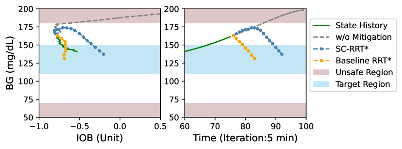
Figure 7: Example Mitigation Paths by SC-RRT* and Baseline RRT* Algorithms in the State Space (Left) and Time Space (Right).

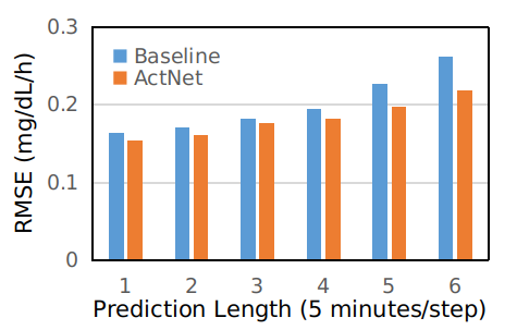
Figure 8: Performance of Control Action Generation (ActNet).

4.7 Evaluation of Response Action Generation

Fig. 8 presents the performance of the response action generation models with and without the integration of HMS knowledge in accurately reconstructing the control action sequence and replicating the controller dynamics. We see that the ML model trained using the proposed custom loss function (Eq. 13) (ActNet) maintains a lower RMSE than the baseline LSTM model for all the prediction lengths, indicating the advantage of combining knowledge and data in accurately generating mitigation/recovery actions.

TABLE VII: Mitigation Performance and Time Overhead of KnowSafe vs. Baselines. The severity of hypoglycemia (BG<70 $mg/dL$) increases with decreasing BG value, including mild (54 $mg/dL$<BG<70 $mg/dL$) and more severe (BG<54 $mg/dL$) categories.

Method	No. Sim.	Out-of-Safe-Range Rate			MSR (Mitigation Success Rate)	Time Overhead (ms)
		BG>180 $mg/dL$	BG<70 $mg/dL$	BG<54 $mg/dL$		Normal Mode	Mit. Mode
KnowSafe	6,545	428 (6.5%)	44 (0.7%)	0	92.8%	46.5	54 or 0
LSTM-RRT	6,545	2492 (38.1%)	603 (9.2%)	66 (1%)	52.7%	46.2	81.5 or 0
Rule-based	6,545	1421 (21.7%)	1792 (27.4%)	370 (5.7%)	50.9%	0.1 (106.5 $\mu$s)	0.1 (121.5 $\mu$s)
Model-based	6,545	1481 (22.6%)	3685 (56.3%)	716 (10.9%)	21.1%	87.9	87.9
FFC	6,545	499 (7.6%)	459 (7.0%)	39 (0.6%)	85.4%	28.8	28.8
Pred-LSTM	6,545	467 (7.1%)	285 (4.4%)	0	88.5%	46.5	28.7

We also observe that the RMSE of the ActNet is slightly lower than that of the baseline for the one-step prediction. However, with the increase in the prediction length, the difference between the ActNet and baseline increases as well. This is because the integrated domain knowledge is independent of the data and prediction length. This observation demonstrates more obvious benefit of integrating domain knowledge on context-specific mitigation actions with ML models for improving sequential prediction accuracy than single value regression, maintaining a stable and low RMSE, and reducing the performance degradation.

Furthermore, the integrated domain knowledge (HMS) helps improve the explainability of black-box ML models in safety-critical CPS, as it offers a reason for selecting a corrective control action under a given context and can be used for run-time verification of the ML model outputs.

4.8 End-to-End Safety Engine Evaluation

We integrate the proposed safety engine (the pipeline of PredNet, SC-RRT*, ActNet models) as well as several state-of-the-art baselines with the controllers in our closed-loop testbed and compare their performances.

4.8.1 Baselines

We compare our combined knowledge and data-driven approach, KnowSafe, to solely knowledge-driven and data-driven approaches by designing different baselines, including a rule-based approach that uses the same domain knowledge on constraints and mitigation actions as KnowSafe, a model-based approach, and ML-based approaches that share the same architecture.

The rule-based baseline includes (i) an anomaly detection algorithm designed based on the context-dependent specification of unsafe control actions and (ii) a mitigation algorithm developed based on the generated HMS in Table II. The detection rules specify whether a control action issued by the controller under a given context might result in transition into the unsafe region. The mitigation rules specify the corrective actions to be taken in each context to stay within the safe region.

We re-implement state-of-the-art defense solutions (e.g., CI [8] or SAVIOR [7]) as a model-based baseline using a dynamic model of the physical system (patient physiology), called the Bergman & Sherwin model [70], to estimate the possible BG value ($BG_{t+1}$) after executing the pump’s command ($u_{t}$) on the patient’s current state ($BG_{t}$). If the predicted BG value goes beyond the patient’s normal range ([70,180] mg/dL, as defined by the medical guidelines), a mitigation algorithm similar to the rule-based mitigation will issue a corrective action that replaces the control action by the controller until the system state returns to the target range.

We also design two solely data-driven baseline models. The first baseline is developed by integrating LSTM models and RRT* with the same architecture as KnowSafe but without the integration of domain-specific knowledge (referred to as LSTM-RRT). For the LSTM models, this is equivalent to setting $\eta$ to be 1 in Eq. 4 and Eq. 13. The second data-driven model directly maps the sensor measurement to the control output $y_{ML}$ with a single regression model, created based on a feed-forward control (FFC) method proposed by [19] for unmanned vehicles. In this approach, when the accumulated error between the ML output and the controller output exceeds a preset threshold, the mitigation mode is activated, and the controller output is replaced by the ML output to be delivered to the actuator. (Note that since these previous works are not directly transferable to APS, we re-implement their high-level pipeline but customize their models and parameters.)

To evaluate the effectiveness of the proposed hazard mitigation module, we design another baseline, Pred-LSTM, that has the same prediction module (PredNet) as KnowSafe but utilizes a single LSTM model (with HMS integration) to generate corrective control actions (without path planning part). The details of each baseline are shown in Fig. 5.

4.8.2 Mitigation Outcome

We rerun all the hazardous simulations (6,545 in both simulators) with different safety engines (KnowSafe vs. baselines) and present their performance in mitigating hazards and maintaining the system inside the safe region in Table VII.

We see that the rule-based baseline mitigates 50.9% of the hazards, but fails to keep the remaining half of the simulations within the safe region. Similarly, the LSTM-RRT baseline successfully prevents 52.7% of the hazards but has 3,095 simulations outside the safe region. This is because while the rule-based strategy knows about the context, the generated high-level mitigation action does not infer specific quantitative values for mitigating potential hazards. In contrast, the ML baseline outputs more specific mitigation actions but relies on a black-box data-driven model that may violate HMS rules under a given context. Therefore, by combining the knowledge with data, KnowSafe overcomes the shortage of either approach and utilizes the advantages of both methods, achieving at least 41.9% higher success rate than solely rule-based and ML-based (LSTM-RRT) baselines and keeping the number of out-of-safe-range simulations low.

We also observe that KnowSafe outperforms the model-based and FFC baselines by achieving the highest MSR and the fewest simulations with BG outside the target range. In addition, BG goes below 54 $mg/dL$ in 39 and 716 simulations with FFC and model-based mitigation, respectively, which may result in severe hypoglycemia and serious complications (e.g., seizure, coma, or even death). In contrast, KnowSafe keeps the BG above 54 $mg/dL$ for all the simulations. Although BG goes below 70 $mg/dL$ in 44 simulations with KnowSafe, the percentage is much lower than the baselines and is much less concerning than the cases with BG below 54 $mg/dL$.

The better performance of the proposed mitigation approach over these baselines might be because our approach aims to be early in hazard prediction and mitigation by estimating the possibility of the system state entering the unsafe region. In contrast, approaches like the FFC and model-based baselines detect the hazards after they occur or wait until the error between the ML predictions and the actual system states or outputs exceeds a noticeable threshold, which wastes the limited mitigation time budget on hazard detection and may lead to mitigation/recovery failure.

Although Pred-LSTM has the same prediction module with KnowSafe and shares the same benefit of early hazard prediction, its overall MSR is 4.3% lower. This result demonstrates the advantage of our hazard mitigation pipeline (SC-RRT* and ActNet) over a single ML model that directly outputs a control action based on current system states since SC-RRT* can find an optimal mitigation path while Pred-LSTM can only generate a single-step mitigation action at each control cycle. Since Pred-LSTM has the same prediction module as KnowSafe, we don’t compare its performance in the following sections.

TABLE VIII: Average BG Value and Max Deviations in the Adverse Event Simulations with No Mitigation or with KnowSafe.

Metric	Max Deviation ($mg/dL$)		Average BG ($mg/dL$)
	Above 180	Below 70
Simulations w/o Mitigation	175.3	49.6	97.3
Simulations with KnowSafe	21.6	4.3	128.9

Table VIII also shows the maximum deviations of BG from the safe region boundaries in each simulation with or without the proposed safety engine. The maximum deviation from the lower bound of the safe region is reduced from 49.6 $mg/dL$ to 4.3 $mg/dL$ (91.3% lower). Similarly, the maximum deviation from the upper bound of the safe region is reduced from 175.3 $mg/dL$ to 21.6 $mg/dL$ (87.6% lower). Therefore, KnowSafe maintains a BG level between the range of [65.7, 201.6] with an average value of 128.9 $mg/dL$ inside the target range, successfully preventing all the hypoglycemia and hyperglycemia hazards.

4.8.3 Timeliness

Fig. 9 presents the timeliness of each mitigation strategy in predicting potential hazards measured by the average reaction time. We have the following observations:

• The model-based baseline keeps the lowest reaction time and MSR (see Table VII), indicating that sufficient reaction time is necessary for effective mitigation/recovery.

• The LSTM-RRT baseline achieves a similar reaction time as KnowSafe and 1.4 times higher MSR than the model-based approach, further attesting to the benefit of early hazard prediction. However, the LSTM-RRT baseline still needs to be revised to mitigate the remaining 49.1% hazards, indicating that solely being early is not enough to guarantee mitigation success.

• The rule-based baseline has a smaller reaction time than the LSTM-RRT approach but achieves a similar MSR, indicating that being context-aware improves mitigation performance.

• The FFC baseline achieves the largest reaction time by generating alerts across the entire simulation period, which would bother the users and may result in unnecessary mitigation. We will further analyze such false positive rates in the following subsection.

• KnowSafe maintains a stable and sufficient reaction time and achieves the highest MSR, demonstrating the advantage of combining domain-specific knowledge with data in being both context-aware and early in the prediction of hazards for successful mitigation/recovery.

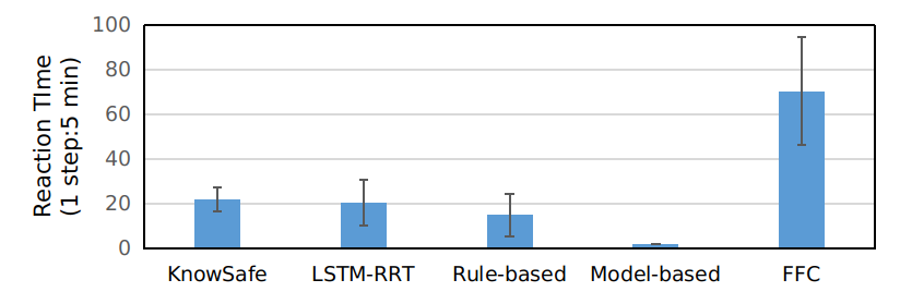
Figure 9: Reaction Time of Each Mitigation Strategy.

4.8.4 False Positives

We also evaluate the consequences of the unwanted mitigation actions activated by false alarms of each mitigation strategy by running it with all the non-hazardous simulations (11,095 in both simulators). We see in Fig. 10 that the FFC baseline is falsely activated for 96.9% simulations and results in 21.3% new hazards, which indicates the drawbacks of such a single ML model in accurately detecting and mitigating hazards. The LSTM-RRT baseline achieves a lower FPR and new hazard rate than the model-based and FFC baselines, indicating the benefit of the proposed hazard prediction and mitigation pipeline. The rule-based safety engine gets two times of false positives than the LSTM-RRT one but keeps the new hazard rate much lower, demonstrating the low risk of the generated HMS even with false activation. KnowSafe maintains the lowest FPR (5.4%) without introducing any new hazards, attesting to the advantage of combining domain knowledge with data-driven techniques in reducing the FPR and the risk of introducing new hazards in the hazard prediction and mitigation process.

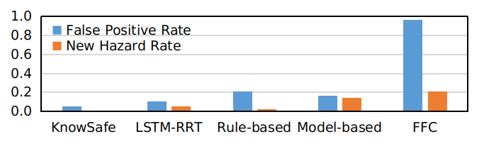
Figure 10: Performance of Different Safety Engines in 11,095 Non-Hazardous Simulations.

4.9 Mitigation of Stealthy Attacks

To evaluate the performance of the proposed mitigation strategy against stealthy attacks, we assume a powerful attacker who knows the mitigation mechanism, including the ML architecture and parameters. We rerun the experiments shown in Table III, in which the attacker stops the attack action (or injection of faults) to stay stealthy when such action will trigger the mitigation alarms if launched. We compare the performance with a model-based baseline (similar to existing solutions CI and SAVIOR) and an ML-based baseline (e.g., LSTM-RRT introduced in Section 4.8.1). We do not test the FFC baseline due to its high false positive rates.

TABLE IX: Performance of Each Mitigation Strategy against Stealthy Attacks.

Method	No. Simulation Out of Safe Range [70,180] mg/dL	Max Deviation (mg/dL)
		Above 180	Below 70
KnowSafe	0	0	0
LSTM-RRT	2,958	45.3	15.9
Model-based	5,026	74.6	26.5

In Table IX, we see that the success rate of KnowSafe under stealthy attacks is 100%, and BG values are kept within the safe range [70,180] $mg/dL$ in all the simulations with both the Glucosym simulator and the UVA-Padova simulator. In comparison, the model-based approach fails to mitigate the stealthy attack in 5,026 simulations (76.8% of 6,545 hazardous cases in Table VII) with a max deviation of 74.6 $mg/dL$ above 180 $mg/dL$ and 26.5 $mg/dL$ below 70 $mg/dL$. This is because the model-based approach can only predict the system state in the next time step, which is not sufficient to prevent or mitigate hazards under stealthy attacks. On the other hand, the ML-based approach LSTM-RRT reduces max deviations to 45.3 $mg/dL$ above 180 $mg/dL$ and 15.9 $mg/dL$ below 70 $mg/dL$ but still fails to mitigate 2,958 (45.2%) stealthy attacks due to unconstrained predictions.

In contrast, the proposed KnowSafe overcomes these problems by combining knowledge and data that can accurately predict system states in the following two hours, which thus ensures enough reaction time and a high success rate in mitigating stealthy attacks.

4.10 Resource Utilization

We evaluate the resource utilization of the proposed approaches in the closed-loop simulation. We run the simulations with different safety engines or without any mitigation/recovery 1,000 times and calculate the average time overhead. Results in Table VII show that KnowSafe introduces an average overhead of 46.5 ms (PredNet) during normal operation and before entering mitigation mode and 54 ms (SC-RRT* 25.3 ms, ActNet 28.7 ms) when in the mitigation mode. These overheads are much smaller than the control cycle period in APS (5 minutes), and thus will not severely affect the system operation at run-time. Note that KnowSafe does not introduce any time overhead after entering the mitigation mode when no updates to the corrective actions are made (see lines 9-13 in Algorithm 2). The LSTM-RRT baseline has a similar time overhead for hazard prediction and mitigation but a slightly larger overhead for the baseline RRT* algorithm (52.8 ms) as more nodes are found and processed due to looser constraints. In contrast, the overall time overhead of rule-based, model-based, and FFC baselines are 121.5 $\mu$s, 87.9 ms, and 28.8 ms, respectively. This shows that the overhead of KnowSafe is comparable to single models used in model-based and FFC baselines.

We also evaluate the resource utilization of KnowSafe on an actual typical MCU used in APS (Raspberry Pi 4 with 8GB RAM as shown in Fig. 5) with optimized ML implementation [75]. We observe a time overhead of 18 $\mu$s ($4.12\times 10^{-7}$% of the normal execution time of 4.36s) and 25.3 ms ($5.8\times 10^{-5}$%) before and after entering the mitigation mode, respectively, and the peak memory usage increase is 38MB (0.48% of the available 8GB RAM).

5 Discussion

Sensor Perturbations: This paper mainly focuses on accidental faults or malicious attacks targeting the CPS controller. Any perturbations in the sensor data will potentially affect the safety engine’s performance. However, benefiting from the knowledge of data and model properties, the proposed PredNet can construct a sequence of system states with a low RMSE (e.g., 0.38 $mg/dL$ in APS), which can be used to detect sensor compromise (similar to [11, 7]) and generate mitigation/recovery actions for a considerable period. Previous work has also shown that integrating domain knowledge with ML anomaly detection can improve the robustness against small perturbations on ML inputs without sacrificing accuracy and transparency [21].

Sim-to-Real Gap: The differences between the simulation and the actual implementation in the real world might also threaten the validity of the proposed method. We try to reduce the sim-to-real gap by using real control software (used with actual diabetic patients [76, 77]), real patient simulators that are either approved by the FDA for clinical testing or use actual patient profiles [69, 70], and a realistic adverse event simulator. Furthermore, a publicly-available dataset collected from a clinical trial [22] and an actual implementation on a typical APS MCU are used to further attest to the effectiveness/validity of the proposed approach.

Generalization and Limitation: We demonstrate the effectiveness of the proposed approach in two closed-loop APS testbeds and a real clinical dataset, but several limitations narrow the generalization of our approach. Specifically, our approach is limited to the CPS in which the system state can be represented by a subset of state variables, based on which the safety properties can be formally specified. Also, our approach is limited to CPS, where the control cycle and device memory are larger than this approach’s requirement reported in Section 4.10.

The primary task of adapting our method to a new type of CPS involves creating safety specifications, which may not be easy for more complex systems and might require domain-specific technical expertise. This paper adopts a formal framework that can generate formal safety specifications using a control-theoretic hazard analysis method [6, 66] in cooperation with domain experts. An example of safety specification for Adaptive Cruise Control systems (ACC) for autonomous driving was explored in previous work [66]. Further study of the knowledge specification and hazard mitigation in different systems and scenarios is beyond the scope of the paper.

Real-World Deployment: The proposed approach can be implemented on a smartphone (similar to some commercial APS as shown in Fig. 5) or be integrated with the pump microcontroller, but running ML models on resource-scarce embedded systems might be challenging. However, significant progress has been made in implementing ML models on embedded systems, such as using low-power embedded GPUs [78]), ML accelerators [79], or optimized ML implementations [80, 75]. Further, some high-end MCUs have large memory and powerful computation capabilities [81]. In this paper, we also implemented the proposed method on a typical MCU used in APS (Raspberry Pi 4 with 8GB RAM as shown in Fig. 5) with improved inference time (see Section 4.10). In addition, the integration of domain knowledge with the ML models is done offline during training without adding computational costs at run-time.

Our models are trained on patient/configuration-specific data. Changes in configuration, patient’s physiological, or environmental context necessitate recalibration/retraining.

6 Related work

Anomaly Detection and Attack Recovery: In previous sections, we introduced existing works on anomaly detection and recovery using model-based, rule-based, or ML-based approaches. Our work distinguishes itself from these previous works in combining knowledge with data-driven techniques for preemptive hazard prediction and mitigation with better accuracy and a higher mitigation success rate. Further, this paper focuses on mitigating or recovering the CPS from accidental faults or malicious attacks that directly compromise the controller software or hardware functionality in addition to detecting sensor attacks.

Security of APS: We have discussed the existing APS security work in Section 2.4. To the best of our knowledge, this paper is the first on run-time hazard or attack mitigation in APS.

Knowledge Integration: Integrating expert knowledge into ML has been an active area of research [82]. Previous works have focused on enforcing ML to follow logic rules during the training process through applying soft constraints [83], designing specific logistic circuits [84] and network structures [85], generating graph models [86], or utilizing knowledge distillation [87]. In this paper, we integrate domain-specific knowledge of safety constraints and properties as soft constraints with the multivariate sequential prediction models for anomaly detection and hazard mitigation.

7 Conclusion

This paper proposes a combined knowledge and data driven approach for the design of safety engines that can predict and mitigate hazards in APS. We integrate expert domain knowledge with machine learning through the design of novel custom loss functions that enforce the satisfaction of domain-specific safety constraints during the training process. Experimental results for two closed-loop APS testbeds and a diabetic dataset show that the proposed safety engines achieve increased accuracy in predicting hazards and a higher success rate in mitigating them. Future work will focus on studying the generalization of the proposed approach to other CPS.

Xugui Zhou obtained his B.E. in Automation and M.E. in Control Science and Engineering from Shandong University, China. He is currently a Ph.D. candidate in the Department of Electrical and Computer Engineering at the University of Virginia. Before joining Dependable Systems and Analytics Lab at UVa in January 2019, he was an Project Manager and Engineer at NR Research Institute, State Grid of China. His research interests are at the intersection of computer systems dependability and control system theory and engineering. He is particularly interested in engineering safer autonomous systems through resilience assessment, security validation, and artificial intelligence techniques.

Maxfield Kouzel is an undergraduate student in Computer Science at the University of Virginia. He joined the Dependable Systems and Computing Lab in October 2021, and his research interests center around building more effective and robust autonomous systems with control theory and artificial intelligence.

Chloe Smith received her B.Sc. and M.Sc. in Computer Science from the University of Virginia. Her research interests center around improving the safety and user experience of artificial pancreas systems.

Homa Alemzadeh received her B.Sc. and M.Sc. in Computer Engineering from the University of Tehran and her Ph.D. in Electrical and Computer Engineering from the University of Illinois Urbana-Champaign. She is currently an assistant professor in the department of Electrical and Computer Engineering, with a courtesy appointment in the department of Computer Science at the University of Virginia. She is also affiliated with the LinkLab, a multi-disciplinary center for research and education in Cyber-Physical Systems (CPS). Before joining UVA, she was a research staff member at the IBM T. J. Watson Research Center. Her research interests are at the intersection of computer systems dependability and data science. She is particularly interested in data-driven resilience assessment and design of embedded and cyber-physical systems, with a focus on safety and security validation and monitoring in medical devices and systems, surgical robots, and autonomous systems. She is the recipient of the 2022 NSF CAREER Award and the 2017 William C. Carter Ph.D. Dissertation Award in Dependability from the IEEE TC and IFIP Working Group 10.4 on Dependable Computing and Fault Tolerance.

References

- [1] C. Li, A. Raghunathan, and N. K. Jha, “Hijacking an insulin pump: Security attacks and defenses for a diabetes therapy system,” in 2011 IEEE 13th International Conference on e-Health Networking, Applications and Services. IEEE, 2011, pp. 150–156.
- [2] A. A. Cárdenas, S. Amin, and Z.-S. Lin et al., “Attacks against process control systems: Risk assessment, detection, and response,” in ASIACCS, 2011, p. 12.
- [3] X. Zhou, A. Schmedding, H. Ren, L. Yang, P. Schowitz, E. Smirni, and H. Alemzadeh, “Strategic safety-critical attacks against an advanced driver assistance system,” in 2022 52nd Annual IEEE/IFIP International Conference on Dependable Systems and Networks (DSN). IEEE, 2022, pp. 79–87.
- [4] CVE, “CVE-Insulin-Pump.” 2020. [Online]. Available: https://cve.mitre.org/cgi-bin/cvekey.cgi?keyword=insulin+pump
- [5] X. Zhou, M. Kouzel, H. Ren, and H. Alemzadeh, “Design and validation of an open-source closed-loop testbed for artificial pancreas systems,” in 2022 IEEE/ACM Conference on Connected Health: Applications, Systems and Engineering Technologies (CHASE). IEEE, 2022, pp. 1–12.
- [6] X. Zhou, B. Ahmed, J. H. Aylor, P. Asare, and H. Alemzadeh, “Data-driven design of context-aware monitors for hazard prediction in artificial pancreas systems,” in 2021 51st Annual IEEE/IFIP International Conference on Dependable Systems and Networks (DSN), 2021, pp. 484–496.
- [7] R. Quinonez, J. Giraldo, L. Salazar, E. Bauman, A. Cardenas, and Z. Lin, “SAVIOR: Securing autonomous vehicles with robust physical invariants,” in 29th USENIX Security Symposium (USENIX Security 20). USENIX Association, Aug. 2020, pp. 895–912.
- [8] H. Choi, W.-C. Lee, Y. Aafer, F. Fei, Z. Tu, X. Zhang, D. Xu, and X. Deng, “Detecting attacks against robotic vehicles: A control invariant approach,” in Proceedings of the 2018 ACM SIGSAC Conference on Computer and Communications Security, 2018, pp. 801–816.
- [9] A. Ding, P. Murthy, L. Garcia, P. Sun, M. Chan, and S. Zonouz, “Mini-me, you complete me! data-driven drone security via dnn-based approximate computing,” in 24th International Symposium on Research in Attacks, Intrusions and Defenses, 2021, pp. 428–441.
- [10] R. E. Lyons and W. Vanderkulk, “The use of triple-modular redundancy to improve computer reliability,” IBM journal of research and development, vol. 6, no. 2, pp. 200–209, 1962.
- [11] H. Choi, S. Kate, Y. Aafer, X. Zhang, and D. Xu, “Software-based realtime recovery from sensor attacks on robotic vehicles,” in 23rd International Symposium on Research in Attacks, Intrusions and Defenses (RAID 2020). USENIX Association, Oct. 2020, pp. 349–364.
- [12] Y. Zhang, R. Jetley, P. L. Jones, and A. Ray, “Generic safety requirements for developing safe insulin pump software,” Journal of diabetes science and technology, vol. 5, no. 6, pp. 1403–1419, 2011.
- [13] N. Paul, T. Kohno, and D. C. Klonoff, “A review of the security of insulin pump infusion systems,” Journal of diabetes science and technology, vol. 5, no. 6, pp. 1557–1562, 2011.
- [14] L. Meneghetti, G. A. Susto, and S. Del Favero, “Detection of insulin pump malfunctioning to improve safety in artificial pancreas using unsupervised algorithms,” Journal of diabetes science and technology, vol. 13, no. 6, pp. 1065–1076, 2019.
- [15] A. Desai, S. Ghosh, S. A. Seshia, N. Shankar, and A. Tiwari, “SOTER: a runtime assurance framework for programming safe robotics systems,” in 2019 49th Annual IEEE/IFIP International Conference on Dependable Systems and Networks (DSN). IEEE, 2019, pp. 138–150.
- [16] D. Phan, J. Yang, M. Clark, R. Grosu, J. Schierman, S. Smolka, and S. Stoller, “A component-based simplex architecture for high-assurance cyber-physical systems,” in 2017 17th International Conference on Application of Concurrency to System Design (ACSD), 2017, pp. 49–58.
- [17] L. Zhang, X. Chen, F. Kong, and A. A. Cardenas, “Real-time attack-recovery for cyber-physical systems using linear approximations,” in 2020 IEEE Real-Time Systems Symposium (RTSS), 2020, pp. 205–217.
- [18] L. Zhang, K. Sridhar, M. Liu, P. Lu, X. Chen, F. Kong, O. Sokolsky, and I. Lee, “Real-time data-predictive attack-recovery for complex cyber-physical systems,” in 2023 IEEE 29th Real-Time and Embedded Technology and Applications Symposium (RTAS). IEEE, 2023, pp. 209–222.
- [19] D. Pritam, L. Guanpeng, C. Zitao, K. Mehdi, and P. Karthik, “Pid-piper: Recovering robotic vehicles from physical attacks,” in 2021 51st Annual IEEE/IFIP International Conference on Dependable Systems and Networks (DSN), 2021.
- [20] Y. Luo, Y. Xiao, L. Cheng, G. Peng, and D. D. Yao, “Deep Learning-based Anomaly Detection in Cyber-physical Systems: Progress and Opportunities,” ACM Computing Surveys, vol. 54, no. 5, pp. 106:1–106:36, May 2021.
- [21] X. Zhou, M. Kouzel, and H. Alemzadeh, “Robustness testing of data and knowledge driven anomaly detection in cyber-physical systems,” 5th Annual IEEE/IFIP International Conference on Dependable Systems and Networks Workshop on Dependable and Secure Machine Learning (DSN-DSML), 2022.
- [22] JDRF/NIDDK Artificial Pancreas Project Consortium, “Reduction of Nocturnal Hypoglycemia by Using Predictive Algorithms and Pump Suspension: An Outpatient Pilot Feasibility and Efficacy Study (PSO3),” https://public.jaeb.org/jdrfapp2/stdy/458.
- [23] C. Li, M. Zhang, A. Raghunathan, and N. K. Jha, “Attacking and defending a diabetes therapy system,” Security and Privacy for Implantable Medical Devices, pp. 175–193, 2014.
- [24] D. Goodin. (2011) Insulin pump hack delivers fatal dosage over the air. [Online]. Available: https://www.theregister.com/2011/10/27/fatal_insulin_pump_attack/
- [25] R. Heartfield, G. Loukas, S. Budimir, A. Bezemskij, J. R. Fontaine, A. Filippoupolitis, and E. Roesch, “A taxonomy of cyber-physical threats and impact in the smart home,” Computers & Security, vol. 78, pp. 398–428, 2018.
- [26] C. M. Ramkissoon, B. Aufderheide, B. W. Bequette, and J. Vehí, “A review of safety and hazards associated with the artificial pancreas,” IEEE reviews in biomedical engineering, vol. 10, pp. 44–62, 2017.
- [27] M. Zhang, A. Raghunathan, and N. K. Jha, “Trustworthiness of medical devices and body area networks,” Proceedings of the IEEE, vol. 102, no. 8, pp. 1174–1188, 2014.
- [28] Stilgherrian (CSO Online). (2011) Lethal medical device hack taken to next level: Attacker sniffs insulin pump id, delivers fatal dose. [Online]. Available: http://www2.cso.com.au/article/404909/lethal_medical_device_hack_taken_next_level/
- [29] CVE, “CVE-2018-14781.” 2018. [Online]. Available: https://cve.mitre.org/cgi-bin/cvename.cgi?name=CVE-2018-14781
- [30] D. C. Klonoff, “Cybersecurity for connected diabetes devices,” J Diabetes Sci Technol, vol. 9, no. 5, pp. 1143–1147, 2015.
- [31] D. T. O’Keeffe, S. Maraka, A. Basu, P. Keith-Hynes, and Y. C. Kudva, “Cybersecurity in artificial pancreas experiments,” Diabetes technology & therapeutics, vol. 17, no. 9, pp. 664–666, 2015.
- [32] CVE, “CVE-2019-10964.” 2019. [Online]. Available: https://cve.mitre.org/cgi-bin/cvename.cgi?name=CVE-2019-10964
- [33] N. Asarani, A. Reynolds, M. Elbalshy, M. Burnside, M. De Bock, D. Lewis, and B. Wheeler, “Efficacy, safety, and user experience of diy or open-source artificial pancreas systems: a systematic review,” Acta Diabetologica, vol. 58, pp. 539–547, 2021.
- [34] “Principles of an open artificial pancreas system (openaps),” https://openaps.org/reference-design, 2021.
- [35] D. S. Eng and J. M. Lee, “The promise and peril of mobile health applications for diabetes and endocrinology,” Pediatric diabetes, vol. 14, no. 4, pp. 231–238, 2013.
- [36] K. Knorr and D. Aspinall, “Security testing for android mhealth apps,” in 2015 IEEE Eighth International Conference on Software Testing, Verification and Validation Workshops (ICSTW). IEEE, 2015, pp. 1–8.
- [37] W. B. Glisson, T. Andel, T. McDonald, M. Jacobs, M. Campbell, and J. Mayr, “Compromising a medical mannequin,” arXiv preprint arXiv:1509.00065, 2015.
- [38] A. Chacko and T. Hayajneh, “Security and privacy issues with iot in healthcare,” EAI Endorsed Transactions on Pervasive Health and Technology, vol. 4, no. 14, 2018.
- [39] D. Giansanti and L. Monoscalco, “The cyber-risk in cardiology: Towards an investigation on the self-perception among the cardiologists,” Mhealth, vol. 7, 2021.
- [40] A. Sari and J. Sopuru, “E-health threat intelligence within cyber-defence framework for e-health organizations,” Smart Systems for E-Health: WBAN Technologies, Security and Applications, pp. 161–179, 2021.
- [41] T. Flynn, G. Grispos, W. Glisson, and W. Mahoney, “Knock! knock! who is there? investigating data leakage from a medical internet of things hijacking attack,” 2020.
- [42] Y. Mo and B. Sinopoli, “Integrity attacks on cyber-physical systems,” in Proceedings of the 1st international conference on High Confidence Networked Systems, 2012, pp. 47–54.
- [43] X. Hei, X. Du, S. Lin, and I. Lee, “Pipac: Patient infusion pattern based access control scheme for wireless insulin pump system,” in 2013 Proceedings IEEE INFOCOM. IEEE, 2013, pp. 3030–3038.
- [44] E. Marin, D. Singelée, B. Yang, I. Verbauwhede, and B. Preneel, “On the feasibility of cryptography for a wireless insulin pump system,” in Proceedings of the Sixth ACM Conference on Data and Application Security and Privacy, 2016, pp. 113–120.
- [45] D. C. Klonoff, “Cybersecurity for connected diabetes devices,” Journal of diabetes science and technology, vol. 9, no. 5, pp. 1143–1147, 2015.
- [46] K. Malasri and L. Wang, “Securing wireless implantable devices for healthcare: Ideas and challenges,” IEEE Communications Magazine, vol. 47, no. 7, pp. 74–80, 2009.
- [47] M. M. Kermani, M. Zhang, A. Raghunathan, and N. K. Jha, “Emerging frontiers in embedded security,” in 2013 26th international conference on VLSI design and 2013 12th international conference on embedded systems. IEEE, 2013, pp. 203–208.
- [48] J. A. Tamada, M. Lesho, and M. J. Tierney, “Keeping watch on glucose,” Ieee Spectrum, vol. 39, no. 4, pp. 52–57, 2002.
- [49] “Common Vulnerabilities and Exposures Database.” [Online]. Available: https://cve.mitre.org/
- [50] N. Leveson and J. Thomas, “An STPA primer,” Cambridge, MA, 2013.
- [51] S. A. Brown, B. P. Kovatchev, D. Raghinaru, J. W. Lum, B. A. Buckingham, Y. C. Kudva, L. M. Laffel, C. J. Levy, J. E. Pinsker, R. P. Wadwa et al., “Six-month randomized, multicenter trial of closed-loop control in type 1 diabetes,” vol. 381, no. 18. Mass Medical Soc, 2019, pp. 1707–1717.
- [52] U. Pedersen-Bjergaard and B. Thorsteinsson, “Reporting severe hypoglycemia in type 1 diabetes: facts and pitfalls,” Current Diabetes Reports, vol. 17, pp. 1–11, 2017.
- [53] H. Alemzadeh, D. Chen, and X. Li et al., “Targeted attacks on teleoperated surgical robots: Dynamic model-based detection and mitigation,” in 2016 46th Annual IEEE/IFIP International Conference on DSN). IEEE, 2016, pp. 395–406.
- [54] N. Oliver, M. Reddy, C. Marriott, T. Walker, and L. Heinemann, “Open source automated insulin delivery: addressing the challenge.” npj Digit. Med., vol. 2, no. 124, 2019.
- [55] T. Dehling, F. Gao, S. Schneider, A. Sunyaev et al., “Exploring the far side of mobile health: information security and privacy of mobile health apps on ios and android,” JMIR mHealth and uHealth, vol. 3, no. 1, p. e3672, 2015.
- [56] U.S. Food and Drug Administration, “Class 2 device recall medtronic minimed paradigm model mmt723k insulin pump,” https://www.accessdata.fda.gov/scripts/cdrh/cfdocs/cfRES/res.cfm?id=175210, March 16, 2021.
- [57] E. Chien, L. OMurchu, and N. Falliere, “W32.duqu: The precursor to the next stuxnet,” in 5th USENIX Workshop on Large-Scale Exploits and Emergent Threats (LEET 12), San Jose, CA, 2012.
- [58] K. Zetter, “It’s insanely easy to hack hospital equipment,” Wired Magazine, vol. 16, no. 1, pp. 303–336, 2014.
- [59] “Arm trustzone technology,” https://developer.arm.com/ip-products/security-ip/trustzone.
- [60] H. Weng, C. Hettiarachchi, C. Nolan, H. Suominen, and A. Lenskiy, “Ensuring security of artificial pancreas device system using homomorphic encryption,” Biomedical Signal Processing and Control, vol. 79, p. 104044, 2023.
- [61] M. R. Aliabadi, M. Seltzer, M. V. Asl, and R. Ghavamizadeh, “Artinali#: An efficient intrusion detection technique for resource-constrained cyber-physical systems,” International Journal of Critical Infrastructure Protection, vol. 33, p. 100430, 2021.
- [62] P. V. Astillo, J. Jeong, W.-C. Chien, B. Kim, J. Jang, and I. You, “Smdaps: A specification-based misbehavior detection system for implantable devices in artificial pancreas system,” Journal of Internet Technology, vol. 22, no. 1, pp. 1–11, 2021.
- [63] O. Vega-Hernandez, F. Campos-Cornejo, D. Campos-Delgado, and D. Espinoza-Trejo, “Increasing security in an artificial pancreas: diagnosis of actuator faults,” in 2009 Pan American Health Care Exchanges. IEEE, 2009, pp. 137–142.
- [64] S. Karaman and E. Frazzoli, “Sampling-based algorithms for optimal motion planning,” The international journal of robotics research, vol. 30, no. 7, pp. 846–894, 2011.
- [65] E. Bartocci, “Monitoring, learning and control of cyber-physical systems with stl (tutorial),” in Runtime Verification: 18th International Conference, RV 2018, Limassol, Cyprus, November 10-13, 2018, Proceedings 18. Springer, 2018, pp. 35–42.
- [66] X. Zhou, B. Ahmed, J. H. Aylor, P. Asare, and H. Alemzadeh, “Hybrid knowledge and data driven synthesis of runtime monitors for cyber-physical systems,” IEEE Transactions on Dependable and Secure Computing, 2023.
- [67] E. Chertok Shacham, H. Kfir, N. Schwartz, and A. Ishay, “Glycemic control with a basal-bolus insulin protocol in hospitalized diabetic patients treated with glucocorticoids: a retrospective cohort,” BMC Endocr Disord, vol. 18(75), pp. 1472–6823, 2018.
- [68] “Glucosym,” https://github.com/Perceptus/GlucoSym.
- [69] C. D. Man, F. Micheletto, D. Lv, M. Breton, B. Kovatchev, and C. Cobelli, “The UVA/PADOVA type 1 diabetes simulator: new features,” Journal of diabetes science and technology, vol. 8, no. 1, pp. 26–34, 2014.
- [70] S. Kanderian, S. Weinzimer, and G. Voskanyan et al, “Identification of intraday metabolic profiles during closed-loop glucose control in individuals with type 1 diabetes.” Journal of diabetes science and technology, vol. 3, no. 5, pp. 1047–1057, 2009.
- [71] R. Visentin, C. Dalla Man, B. Kovatchev, and C. Cobelli, “The university of Virginia/Padova type 1 diabetes simulator matches the glucose traces of a clinical trial,” Diabetes technology & therapeutics, vol. 16, no. 7, pp. 428–434, 2014.
- [72] R. Hawkins, C. Paterson, C. Picardi, Y. Jia, R. Calinescu, and I. Habli, “Guidance on the assurance of machine learning in autonomous systems (amlas),” arXiv preprint arXiv:2102.01564, 2021.
- [73] J. Xie. (2018) Simglucose v0.2.1. [Online]. Available: https://github.com/jxx123/simglucose
- [74] S. Dutta, T. Kushner, and S. Sankaranarayanan, “Robust data-driven control of artificial pancreas systems using neural networks,” Computational Methods in Systems Biology, vol. 11095, 2018.
- [75] Google Brain team, “TensorFlow Lite for Microcontrollers.” 2019. [Online]. Available: https://www.tensorflow.org/lite/microcontrollers
- [76] D. M. Lewis, “Do-it-yourself artificial pancreas system and the openaps movement,” Endocrinology and Metabolism Clinics, vol. 49, no. 1, pp. 203–213, 2020.
- [77] D. Lewis, S. Leibrand, and O. Community, “Real-world use of open source artificial pancreas systems,” Journal of diabetes science and technology, vol. 10, no. 6, pp. 1411–1411, 2016.
- [78] Neha Rastogi, “Microchip unveils industry’s first MCU with integrated 2d gpu and ddr2 memory.” 2019. [Online]. Available: https://www.engineersgarage.com/microchip-unveils-industrys-first-mcu-with-integrated-2d-gpu-and-ddr2-memory/
- [79] STMicroelectronics, “ISM330DHCX: machine learning core.” 2019. [Online]. Available: https://www.st.com/content/ccc/resource/technical/document/application_note/group1/60/c8/a2/6b/35/ab/49/6a/DM00651838/files/DM00651838.pdf/jcr:content/translations/en.DM00651838.pdf
- [80] C. Gupta, A. S. Suggala, A. Goyal, H. V. Simhadri, B. Paranjape, A. Kumar, S. Goyal, R. Udupa, M. Varma, and P. Jain, “Protonn: Compressed and accurate knn for resource-scarce devices,” in International conference on machine learning. PMLR, 2017, pp. 1331–1340.
- [81] Rhonda Dirvin, “Next-generation armv8.1-m architecture: Delivering enhanced machine learning and signal processing for the smallest embedded devices.” 2019. [Online]. Available: https://www.arm.com/company/news/2019/02/next-generation-armv8-1-m-architecture
- [82] L. Von Rueden, S. Mayer, K. Beckh, B. Georgiev, S. Giesselbach, R. Heese, B. Kirsch, J. Pfrommer, A. Pick, R. Ramamurthy et al., “Informed machine learning-a taxonomy and survey of integrating knowledge into learning systems,” arXiv preprint arXiv:1903.12394, 2019.
- [83] J. Xu, Z. Zhang, T. Friedman, Y. Liang, and G. V. den Broeck, “A semantic loss function for deep learning with symbolic knowledge,” 2018.
- [84] Y. Liang and G. Van den Broeck, “Learning logistic circuits,” in Proceedings of the AAAI Conference on Artificial Intelligence, vol. 33, no. 01, 2019, pp. 4277–4286.
- [85] B. Chen, Z. Hao, X. Cai, R. Cai, W. Wen, J. Zhu, and G. Xie, “Embedding logic rules into recurrent neural networks,” IEEE Access, vol. 7, pp. 14 938–14 946, 2019.
- [86] S. Guo, Q. Wang, L. Wang, B. Wang, and L. Guo, “Jointly embedding knowledge graphs and logical rules,” in Proceedings of the 2016 conference on empirical methods in natural language processing, 2016, pp. 192–202.
- [87] J. Gou, B. Yu, S. J. Maybank, and D. Tao, “Knowledge distillation: A survey,” International Journal of Computer Vision, vol. 129, no. 6, pp. 1789–1819, 2021.