NRTidalv3: A New and Robust Gravitational-Waveform Model for High-Mass-Ratio Binary Neutron Star Systems with Dynamical Tidal Effects

Abstract

For the analysis of gravitational-wave signals, fast and accurate gravitational-waveform models are required. These enable us to obtain information on the system properties from compact binary mergers. In this article, we introduce the NRTidalv3 model, which contains a closed-form expression that describes tidal effects, focusing on the description of binary neutron star systems. The model improves upon previous versions by employing a larger set of numerical-relativity data for its calibration, by including high-mass ratio systems covering also a wider range of equations of state. It also takes into account dynamical tidal effects and the known post-Newtonian mass-ratio dependence of individual calibration parameters. We implemented the model in the publicly available LALSuite software library by augmenting different binary black hole waveform models (IMRPhenomD, IMRPhenomX, and SEOBNRv5_ROM). We test the validity of NRTidalv3  by comparing it with numerical-relativity waveforms, as well as other tidal models. Finally, we perform parameter estimation for GW170817 and GW190425 with the new tidal approximant and find overall consistent results with respect to previous studies.

I Introduction

Two years after the discovery of a binary black hole (BBH) merger [1], which initiated the era of gravitational-wave (GW) astronomy, the discovery of the binary neutron star (BNS) merger GW170817 inaugurated a new era in multi-messenger astronomy [2, 3, 4], in which GWs and electromagnetic signals are combined to unravel these highly energetic events. Indeed, the GW detection of GW170817 came along with electromagnetic signatures covering the whole frequency range from radio to gamma-rays [3, 4]. However, GW170817 was just the beginning. Two years later, the LIGO-Virgo-Kagra collaboration detected the BNS GW190425 [5] and with the increasing sensitivity of current GW detectors as well as planned new-generation detectors, it is expected that the number of BNS events observed will increase in the future [6, 7, 8, 9].

One of the key scientific achievements of GW170817 was the improved knowledge of neutron star (NS) interior [2, 10]. The structure of the NS is primarily described by an equation of state (EoS) of neutron-rich supranuclear-dense matter [11, 12]. In fact, matter in the core of NSs is thought to be at least a few times denser than the nuclear saturation density $\rho\sim 10^{14}\,{\rm g/cm^{3}}$, and there are various (competing) theoretical and phenomenological models in nuclear physics (e.g., [13, 14, 15, 16, 11, 17, 18, 19]) describing this state of matter.

Given that the EoS describing the NS interior influences the tidal deformability, which is a measure of the star’s deformation in response to an external tidal field (e.g., during the gravitational interaction with another compact object [20, 21]), BNS merger observations will shed light on the behavior of matter at extreme densities [20, 22, 2, 23, 5].

Physical parameters of the system, such as mass, spin, and tidal deformabilities, can be extracted from GW signals by comparing the observed data with theoretical predictions obtained by solving the Einstein field equations (EFEs), usually through Bayesian analysis [24, 25]. In principle, ab-initio, numerical-relativity (NR) simulations which solve the EFEs on supercomputers would be the method of choice for the description of a BNS waveform. However, such simulations come with high computational costs and typically only cover the late stage of the inspiral and merger [26, 27, 28, 29, 30, 31, 32, 33]. Furthermore, these simulations are also characterized by an intrinsic uncertainty due to the numerical discretization that is employed to solve the EFEs.

Over the years, the community has developed different waveform models for BNS systems. One class of models is based on post-Newtonian (PN) theory, which expands the EFEs in powers of $v/c$, where $v$ is the binary characteristic velocity and $c$ is the speed of light. These approximants include tidal interactions that start at the 5th PN order [34] ($\propto({{v}/{c}})^{10}$) up to 7.5PN order [35, 36, 37], which is the highest PN order that is currently known for tidal effects. However, even high-PN approximants are still not accurate enough in describing the full GW signal, particularly in the late inspiral shortly before the merger, when the velocities of the objects are larger, and the distance between the stars is smaller. One approach for improving the accuracy of PN predictions is made by using the effective-one-body (EOB) formalism [38, 39, 40, 41, 42]. Over the years, two different ‘families’ of tidal EOB models have emerged: SEOBNRv4T [43, 44] and TEOBResumS [45, 46, 47]. Generally, tidal EOB models are more accurate than PN predictions and allow, in most cases, a reliable description (within the uncertainty of NR simulations) of the GW signal up to the merger of the stars. To avoid the increase in computational costs, which comes naturally when using EOB (as these models solve ordinary differential equations) instead of PN approximations, people have introduced reduced-order models (ROM) [48, 49], post-adiabatic approximations [50, 51], machine learning techniques [52], or a combination of the stationary phase and post-adiabatic approximations [53].

Finally, phenomenological GW models [54, 55] also exist, which incorporate EOB and/or NR data with the aim to model the tidal phase contribution during the coalescence as accurately as possible while still being fast and efficient (e.g. through the use of closed-form analytical expressions for the tidal contribution itself) [56, 28]. One such model is called NRTidal [56], which extracts information from NR, EOB, and PN and constructs an analytical tidal contribution that augments a given BBH waveform baseline, either from EOB models or phenomenological models (such as PhenomD and PhenomX). Two NRTidal versions (NRTidal [56] and NRTidalv2 [57]) have been implemented in the LIGO Algorithm Library (LAL) [58]. The second iteration, NRTidalv2, builds upon NRTidal by using improved NR data, adding amplitude corrections to the GW signal, as well as incorporating spin effects [57]. Though computationally efficient, both NRTidal models come with certain caveats. First, both versions only include equal-mass systems in the calibration of their fitting parameters. Second, the models consider the tidal bulge $Q_{ij}$ of the star to be directly related to the tidal field $\mathcal{E}_{ij}$ generated by its companion via a parameter $\lambda$ known as the tidal deformability, i.e., $Q_{ij}=\lambda\mathcal{E}_{ij}$. In this case, the former NRTidal models considered only adiabatic tides ($\lambda={\rm const.}$) throughout the duration of the inspiral [56, 57]. However, it has been shown that dynamical tides (implying a non-constant, frequency-dependent $\lambda$) can arise from these systems due to the quadrupolar fundamental oscillation mode of the stars [59, 20, 43, 44], see also Refs. [60, 61, 62, 63, 64, 65, 66, 67, 68].

Given these limitations, the aim of this work is to extend the existing NRTidal model. In particular, this new model, called NRTidalv3, includes the following improvements:

1. a larger set of NR BNS waveforms; in total, we utilize 55 waveforms from BAM [31, 33, 32] and SACRA [69, 28] including various total masses, EoSs, mass ratios;

2. inclusion of mass-ratio dependence of the fitting parameters in the calibrated model; and

3. dynamical tides [20, 43, 44, 60].

The paper is organized as follows. In Sec. II, we discuss the employed NR data and the hybridization of the NR data with SEOBNRv4T to construct the hybrid waveforms that are used for the calibration. Sec. III introduces the time-domain NRTidalv3 phase, while Sec. IV discusses the frequency-domain phase. We discuss the implementation and tests for the validation of the model in LAL in Sec. V. We then conduct a parameter estimation analysis of the model with existing GW observations in Sec. VI. Finally, our main conclusion and recommendations are discussed in Sec. VII. Throughout the paper, we use geometric units, where $G=c=1$, unless otherwise stated. For the individual components of the BNS, we define $M_{A}$ to be the primary mass (mass of the heavier companion), $M_{B}$ to be the mass of the secondary companion, each with tidal deformability $\Lambda_{A}$ and $\Lambda_{B}$, respectively. The total mass is given by $M=M_{A}+M_{B}$ and the mass ratio is defined as $q=M_{A}/M_{B}\geq 1$. The aligned spin components are denoted by $\chi_{A}$ and $\chi_{B}$.

II Numerical Relativity Data and Extraction of Tidal Phase Contributions

The NRTidal model is a closed-form GW model that describes the tidal effects in the inspiral part of BNS coalescences [56, 70, 57]. We start from the GW strain

$$h(t)=A(t)e^{-i\phi(t)},$$ (1)

where $A(t)$ is the amplitude, and time-domain $\phi(t)$ is the phase. We assume that we can decompose the phase as

$$\phi(\hat{\omega})=\phi_{0}(\hat{\omega})+\phi_{\rm SO}(\hat{\omega})+\phi_{\rm SS}(\hat{\omega})+\phi_{\rm S^{3}}(\hat{\omega})+\phi_{T}(\hat{\omega})+...,$$ (2)

where $\hat{\omega}=M\omega=Md\phi/dt=M(2\pi f)$ is the rescaled GW frequency, $\phi_{0}$ denotes the non-spinning point-particle contribution to the total phase, $\phi_{\rm SO}$ denotes the spin-orbit (SO) coupling, $\phi_{\rm SS}$ denotes the spin-spin (SS) interactions (both self-spin and spin interactions), $\phi_{\rm{S}^{3}}$ denotes contributions cubic in spin (S³), and $\phi_{T}$ is the tidal phase contribution [20]. We are neglecting all other (higher-order) spin terms in Eq. (2). Similarly to the time domain, we can also write the frequency-domain strain as

$$\tilde{h}(f)=\tilde{A}(f)e^{-i\psi(f)},$$ (3)

with

$$\psi(f)=\psi_{0}(f)+\psi_{\text{SO}}(f)+\psi_{\text{SS}}(f)+\psi_{\text{S}^{3}}(f)+\psi_{T}(f)+...\ .$$ (4)

The NRTidal model aims at modeling the tidal contributions $\phi_{T}$ and $\psi_{T}$, since, unlike the BBH case, tidal deformabilities are present in BNS and BHNS systems and provide valuable information about the internal composition of the individual stars.

II.1 Numerical relativity data set

Previous versions of the NRTidal model start with the tidal part of the GW constructed by combining EOB and NR waveforms [56, 57]. For the calibration of NRTidalv3, 46 NR waveforms simulated by the SACRA code [69, 28, 29], and 9 waveforms simulated with the BAM code [31, 32, 33] were employed. We provide more detailed information in Appendix A. Overall, the NR dataset covers ten different EoSs with $q\in[1.0,2.0]$ (see Fig. 1).

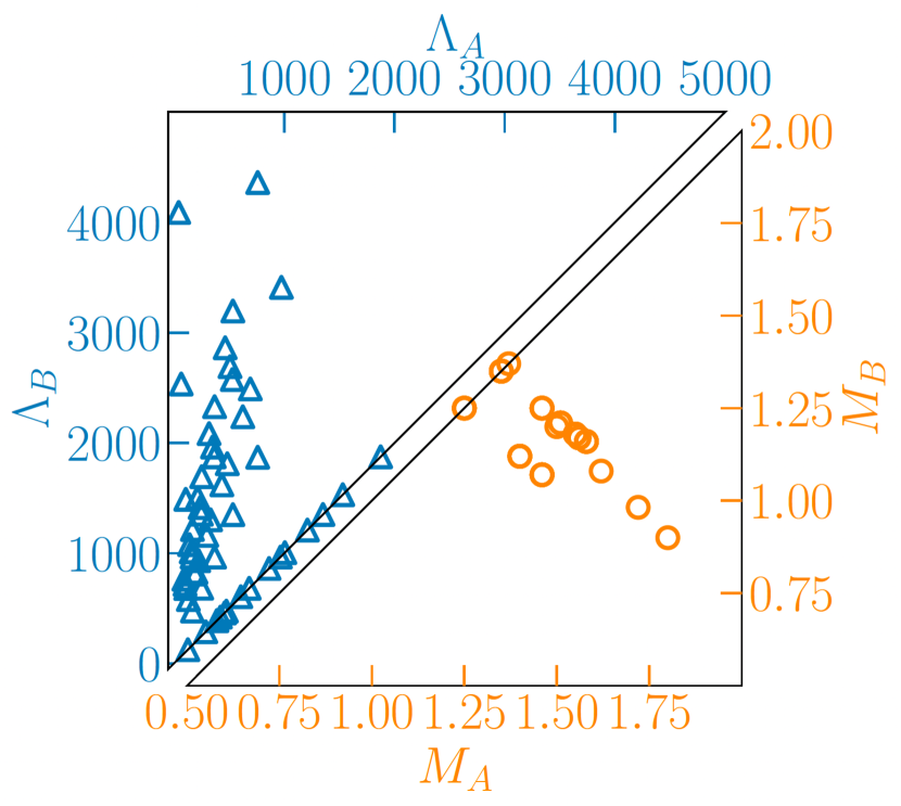
Figure 1: Distribution of the masses (where we set $M_{A}>M_{B}$) and corresponding tidal deformabilities $\Lambda_{A,B}$ of the neutron stars used in the NR simulations (see Table 7). The plot shows overlapping data points for systems with the same masses, but can have different tidal deformabilities due to the various EoSs that were employed.

II.2 Construction of hybrid waveforms

For each of the NR simulations that we employ for calibration, we compute corresponding configurations employing SEOBNRv4T [49] from the LALSuite [58] library. This means that we compute SEOBNRv4T  waveforms including tidal contributions (which we refer to as EOB-BNS later) and without tidal effects, which we call EOB-BBH later. The EOB-BNS waveforms are used in the extraction of the tidal phase contributions, from the early inspiral up to the merger [57]. These tidal phase contributions will then be used in the calibration of NRTidalv3.

For the construction of hybrid waveforms, we first determine the convergence order of the NR data set. If we find a clear convergence order, we construct a higher-order Richardson-extrapolated waveform assuming this convergence order [71, 72]. In our set of waveforms, this is the case for the BAM waveforms from Ref. [57, 32]. For all other data, we are simply employing the highest resolution for the hybrid construction.

In the next step, we align and hybridize the EOB-BNS with the NR waveforms. This is required since our NR data only cover the last few orbits before the merger, but we are planning to construct a closed-form approximant that is valid for the entire frequency range.

For the alignment, we minimize the following integral [26, 27, 73]:

$$\mathcal{I}(\delta t,\delta\phi)=\int_{t_{1}}^{t_{2}}dt|\phi_{\rm NR}(t)-\phi_{\rm EOB}(t+\delta t)+\delta\phi|,$$ (5)

over the chosen frequency interval (or hybridization window, typically near the beginning of the NR waveform) $[\hat{\omega}_{1},\hat{\omega}_{2}]$ corresponding to times $[t_{1},t_{2}]$.

Once the EOB-BNS and the NR waveforms are aligned, we create the hybridized waveform through [26, 27, 73]:

$$h_{\text{EOB-NR}}=\begin{cases}h_{\text{EOB-BNS}},&t\leq t_{1}\\ h_{\text{NR}}H(t)+h_{\text{EOB-BNS}}[1-H(t)],&t_{1}\leq t\leq t_{2}\\ h_{\text{NR}},&t\geq t_{2},\end{cases}$$ (6)

where

$$H(t)\equiv\frac{1}{2}\left[1-\cos\left(\pi\frac{t-t_{1}}{t_{2}-t_{1}}\right)\right],$$ (7)

is the Hann window function. This ensures a smooth transition between the EOB and NR waveforms. The result of this hybridization is shown in Fig. 2 for one example. As indicated above, the final waveforms are labeled EOB-NR.

From the expression of the hybrid waveform above in Eq. (6), we expect the tidal phase contributions of the hybrid to be identical to the one of the EOB-BNS waveform right up to the start of the hybridization window. After the window, the tidal contribution would then be identical to that of the NR waveform. For the purposes of constructing NRTidalv3, we only consider the EOB-NR tidal phase contributions up to merger. The post-merger parts of the EOB-NR phase are not included.

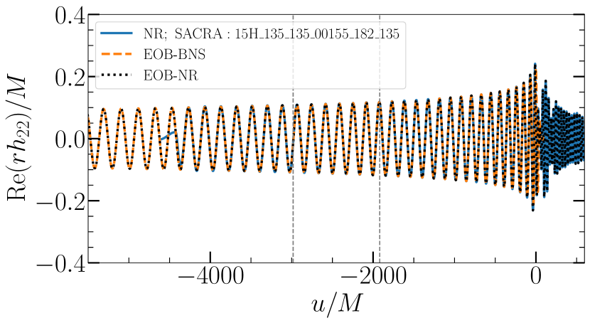
Figure 2: An example of a hybrid Waveform (SACRA:15H_135_135_00155_182_135). Here, we plot the real part of the (2,2) mode $rh_{22}$ of the GW strain (where $r$ is the extraction radius) as a function of the retarded time $u$. The blue curve is the NR waveform, the orange dashed curve is the EOB-BNS waveform from SEOBNRv4T, and the black, dotted curve is the hybridized waveform EOB-NR. The gray, dashed, vertical lines denote the boundaries of the hybridization window, $[t_{1},t_{2}]$ corresponding to $\hat{\omega}\in[0.035,0.04]$. The peak amplitude of the NR and EOB-NR hybrid, indicating merger, is set at $u/M=0$.

II.3 Extracting the tidal phase

In the next step, we extract the tidal phase contribution $\phi_{T}$ up to merger by subtracting the EOB-BBH phase from the EOB-NR phase, which (schematically) means:

$$\phi_{T}=\Delta\phi=\phi_{\text{EOB-NR}}-\phi_{\text{EOB-BBH}}.$$ (8)

Fig. 3 shows the different tidal phase contributions. We find that the resulting $\phi_{T}$ calculated from Eq. (8) has considerable noise, e.g., due to residual eccentricity or remaining density oscillations during the NR simulations. To avoid this, the noise is filtered using a Savitzsky-Golay filter [74, 32] to smoothen the hybrid waveform. This leads to the final tidal phase that we will use as an input for the construction of our NRTidalv3 model.

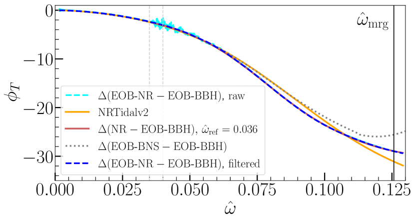
Figure 3: Hybrid tidal phases (EOB -NR) for the configuration SACRA:15H_135_135_00155_182_135. The cyan curve represents the EOB-NR data without applying the smoothening operation indicated in the text, the blue dashed line is EOB-NR after filtering. We also show the phase difference between the pure EOB and NR data, as well as for comparison the NRTidalv2 description. The reference frequency $\hat{\omega}_{\rm ref}$ is used to subtract the EOB-BBH phase from the pure NR phase. Only the hybrid tidal phase up to the merger frequency $\hat{\omega}_{\rm mrg}$ (indicated by a black vertical line) is used in the construction of NRTidalv3.

III Dynamical Tides and the Time Domain NRTidalv3 Phase

III.1 Employed tidal PN knowledge

Our construction of the NRTidalv3 approximant begins with the analytical expression of the time-domain tidal phase contribution through 7.5PN order [36, 37]:

$$\begin{split}\phi_{T}^{\rm PN}=&-\kappa_{A}c_{\text{Newt}}^{A}x^{5/2}\Big{(}1+c_{1}^{A}x+c_{3/2}^{A}x^{3/2}\\ &+c_{2}^{A}x^{2}+c_{5/2}^{A}x^{5/2}\Big{)}+[A\leftrightarrow B],\end{split}$$ (9)

where $x=(\hat{\omega}/2)^{2/3}$, and the $c_{i}$’s are

$$\begin{split}c_{\text{Newt}}^{A}=&\frac{(12-11X_{A})(X_{A}+X_{B})^{2}}{8X_{A}X_{B}^{2}},\\ c_{1}^{A}=&-5\frac{260X_{A}^{3}-2286X_{A}^{2}-919X_{A}+3179}{336(11X_{A}-12)},\\ c_{3/2}^{A}=&-\frac{5}{2}\pi,\\ c_{2}^{A}=&\Big{[}5\big{(}4572288X_{A}^{5}-20427120X_{A}^{4}+158378220X_{A}^{3}+\\ &174965616X_{A}^{2}+43246839X_{A}-387973870\big{)}\Big{]}\\ &/[9144576(11X_{A}-12)],\\ c_{5/2}^{A}=&-\pi\frac{10520X_{A}^{3}-7598X_{A}^{2}+22415X_{A}-27719}{192(11X_{A}-12)},\end{split}$$ (10)

where we also have $A\leftrightarrow B$ and $X_{A,B}=M_{A,B}/M$. Note that the coefficients are different from Ref. [57] in NRTidalv2, which employed the PN expression derived in Ref. [35]. The expression employed for NRTidalv3 uses the updated PN expression introduced in Ref [36, 37]. We also note that the tidal parameters are given by

$$\kappa_{A}=3X_{B}X_{A}^{4}\Lambda_{A},\quad\Lambda_{A}=\frac{k_{2}^{A}}{C_{A}^{5}},$$ (11)

where $C_{A}=M_{A}/R_{A}$ is the compactness of star $A$ in isolation, $R_{A}$ is the radius, and $k_{2}^{A}$ is the tidal Love number of the star [21].

For NRTidalv3, we will incorporate dynamical tides, i.e., $\Lambda_{A,B}$ will be a function of the orbital frequency $\omega_{\text{orb}}=\omega/2$ of the system [44, 63]. This stems from the quadrupolar oscillations of the star due to f-mode excitations, which can be represented by a dynamical quadrupole moment obeying the equation of motion of a tidally driven harmonic oscillator plus relativistic corrections such as redshift, frame-dragging, and spin [44, 62, 63]. The dynamical Love number for nonspinning systems can be approximately expressed in terms of an enhancement factor $k_{\ell}^{\rm eff}$ as $k_{2}\rightarrow k_{2}({\omega})=k_{2}k_{2}^{\rm eff}({\omega})$ (for $\ell=2$), where

$$\begin{split}k_{2}^{\text{eff}}=&u_{2}+v_{2}\Bigg{[}\frac{\omega_{02}^{2}}{\omega_{02}^{2}+(2\omega_{\text{orb}})^{2}}+\frac{\omega_{02}^{2}}{2\sqrt{\epsilon_{2}}\hat{t}|\tilde{\Omega}^{\prime}|(2\omega_{\text{orb}})^{2}}\\ +&\frac{\omega_{02}^{2}}{\sqrt{\epsilon_{2}}(2\omega_{\text{orb}})^{2}}Q_{22}(\hat{t})\Bigg{]},\end{split}$$ (12)

where $\omega_{0\ell}$ is the fundamental mode frequency, $\tilde{\Omega}^{\prime}$ is the derivative (with respect to the gravitational radiation reaction) of the ratio of the mode and tidal forcing frequencies (which in the nonspinning case is $\tilde{\Omega}^{\prime}=-3/8$),

$$\begin{split}Q_{22}(\hat{t})=&\cos(|\tilde{\Omega}^{\prime}|\hat{t}^{2})\int_{-\infty}^{\hat{t}}\sin(|\tilde{\Omega}^{\prime}|s^{2})ds\\ &-\sin(|\tilde{\Omega}^{\prime}|\hat{t}^{2})\int_{-\infty}^{\hat{t}}\cos(|\tilde{\Omega}^{\prime}|s^{2})ds,\end{split}$$ (13)

and

$$\hat{t}=\frac{8}{5\sqrt{\epsilon_{2}}}\left[1-\left(\frac{\omega_{02}}{2\omega_{\text{orb}}}\right)^{5/3}\right],\quad\epsilon_{2}=\frac{256\mu M^{2/3}\omega_{02}^{5/3}}{5\cdot 2^{5/3}},$$ (14)

where $\mu=M_{A}M_{B}/M$ and the quadrupole coefficients are $u_{2}=1/4$ and $v_{2}=3/4$. The enhancement factor Eq. (12) results from a two-timescale approximation for the dynamical tidal quadrupole with a Newtonian estimate for the orbital evolution [44, 63], which should be extended to higher PN orders in future work.

Since $k_{2}^{\text{eff}}$ is a tidal enhancement factor, $k_{2}^{\text{eff}}\rightarrow 1.0$ at $\omega_{\text{orb}}\rightarrow 0$, which means that the tidal deformability of the NS is at its adiabatic value at large distances (i.e., $r\rightarrow\infty)$ from its partner. The fundamental frequency (in kHz) $M_{1.4}f_{02}=(M/1.4M_{\odot})\omega_{02}/(2\pi)$ rescaled to a $1.4M_{\odot}$ NS can be obtained using the quasi-universal relation found in [75]

$$M_{1.4}f_{02}\,[{\rm kHz}]=\sum_{i=0}^{5}g_{i}(\log_{10}\Lambda_{2})^{i},$$ (15)

where

$$\begin{split}g_{i}\in&[4.2590,-0.47874,-0.45353,\\ &0.14439,-0.016194,0.00064163].\end{split}$$ (16)

This relation is shown in Fig. 4 for various values of $\Lambda$, for stars A and B.

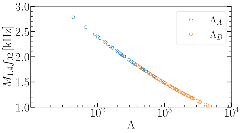
Figure 4: The universal relation between the $f$-mode frequency (in kHz) and $\Lambda$ used for stars A and B.

Then, for $\ell=2$, our tidal parameters for NRTidalv3 contains the modification

$$\kappa_{A,B}\rightarrow\kappa_{A,B}(\hat{\omega})=\kappa_{A,B}k_{2,A,B}^{\text{eff}}(\hat{\omega}).$$ (17)

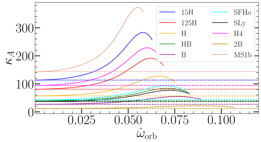
Figure 5: Dynamical tidal parameter in the time-domain as a function of orbital frequency ($\hat{\omega}_{\text{orb}}=\hat{\omega}/2$) for different EoSs, given $q=1.0$. Note that each curve starts at the given constant value of the tidal parameter, which is provided by the dashed lines. The curves terminate at the merger frequency $\hat{\omega}_{\rm mrg}=2\hat{\omega}_{\rm orb}^{\rm mrg}$.

Note that, as constructed, $\kappa$ recovers at large distances (very small frequency) the original (constant) adiabatic value (see Fig. 5).

III.2 Calibrating the time-domain, tidal phase

We then write the effective representation of the time-domain tidal phase in NRTidalv3 as:

$$\phi_{T}^{\text{NRT3}}=-\kappa_{A}(\hat{\omega})c_{\text{Newt}}^{A}x^{5/2}P_{\text{NRT3}}^{A}(x)+[A\leftrightarrow B],$$ (18)

where we use the following functional form

$$\begin{split}&P_{\text{NRT3}}^{A}(x)\\ &=\frac{1+n_{1}^{A}x+n_{3/2}^{A}x^{3/2}+n_{2}^{A}x^{2}+n_{5/2}^{A}x^{5/2}+n_{3}^{A}x^{3}}{1+d_{1}^{A}x+d_{3/2}^{A}x^{3/2}},\end{split}$$ (19)

and the same with $A\leftrightarrow B$. The exact functional form employed in this work is based on numerous tests for various different fitting functions and provided overall the best performance. However, it is clearly an assumption, and also other forms could have been used. We also note that a polynomial form of the fitting function could describe the 55 EOB-NR tidal phase hybrids well, but it is not guaranteed to work for extreme cases, i.e., large masses and/or tidal deformabilities. For some of these configurations, the polynomial can become very large for some mass- and tidal-deformability-dependent combination of coefficients at low frequencies.

Taking the Taylor series expansion of Eq. (18) and comparing it with Eq. (9) allows us to enforce the following constraints to ensure consistency with the PN expression:

$$\begin{split}n_{1}^{A}=&c_{1}^{A}+d_{1}^{A},\\ n_{3/2}^{A}=&\frac{c_{1}^{A}c_{3/2}^{A}-c_{5/2}^{A}-c_{3/2}^{A}d_{1}^{A}+n_{5/2}^{A}}{c_{1}^{A}},\\ n_{2}^{A}=&c_{2}^{A}+c_{1}^{A}d_{1}^{A},\\ d_{3/2}^{A}=&-\frac{c_{5/2}^{A}+c_{3/2}^{A}d_{1}^{A}-n_{5/2}^{A}}{c_{1}^{A}},\end{split}$$ (20)

and similar constraints for $A\rightarrow B$. This means that we are left with six unknown parameters, $(n_{5/2}^{A,B},n_{3}^{A,B},d_{1}^{A,B})$, which can be fitted to the data. However, to make sure that the parameters remain symmetric with respect to stars $A$ and $B$, we can impose additional constraints on these parameters. We find the following functional form to be sufficient for our model:

$$\begin{split}p_{i}^{A,B}(\hat{\omega})=&a_{i,0}+a_{i,1}X_{A,B}\\ &+a_{i,2}(\kappa_{A,B}+1)^{\alpha}\\ &+a_{i,3}X_{A,B}^{\beta},\,\text{for}\,p_{i}\in[n_{5/2},n_{3}],\\ d_{1}^{A,B}=&d_{1,0}+d_{1,1}X_{A,B}+d_{1,2}X_{A,B}^{\beta}.\end{split}$$ (21)

Table 1: Parameters for the NRTidalv3 timed-domain approximant. The table lists the fitting parameters for the Padé approximant, given in Eqs. (19) and (21).

Tides	$k_{2}^{\text{eff}}(\hat{\omega})$ (Eq. (12))
$\alpha$	0.762130731
$\beta$	-0.577611983
	$a_{0}$	$a_{1}$	$a_{2}$	$a_{3}$
$n_{5/2}$	10973.4227	-7775.85588	-0.113688274	-4483.08830
$n_{3}$	-11424.2843	8026.17700	-0.379126345	4665.72647
	$d_{1,0}$	$d_{1,1}$	$d_{1,2}$	-
$d_{1}$	-546.799216	379.280986	223.018238	-

This leaves us with the 13 parameters $a_{i}$’s, $d_{1,i}$’s, $\alpha$, and $\beta$ that we now determine by fitting the function to the EOB-NR hybrid tidal phase data. We note that this parametrization, Eq. (21), should ensure that the coefficients of the Padé approximants themselves are functions of the mass-ratio and tidal deformability, thus making itself applicable to a wide range of EoSs. This is unlike the attempt that was made in Ref. [76] where each set of coefficients ($n$’s and $d$’s) of the Padé approximant in Eq. (19) was specifically determined for two equations of state describing two SpEC waveforms. The parameters for the time-domain NRtidal phase are shown in Table 1.

We show in Fig. 6 the comparison between $\phi_{T}^{\text{NRT3}}$ and the previous versions of the NRTidal model, as well as the 7.5PN approximation of the tidal phase, for the SACRA:15H_125_146_00155_182_135 configuration.

Figure 6: Time-domain tidal phase contributions calculated from different Models for the configuration of the NR waveform SACRA:15H_125_146_00155_182_135. We also show the EOB-NR phase for comparison. The vertical dashed line marks the merger frequency.

The results of the fitting in the time-domain are shown in Fig. 7, together with the fractional differences from the hybridized data. We note the “curving up” of the fits near the merger part of the waveforms; this is primarily due to the dynamical nature of the tides that were incorporated here. For the fits, significant fractional differences $\Delta\phi_{T}/\phi_{T}^{\rm Data}=(\phi_{T}^{\rm NRT3}-\phi_{T}^{\rm Data})/\phi_{T}^{\rm Data}$ are found within the earlier frequencies (where very small phase magnitudes can correspond to large fractional differences) and in the vicinity of the hybridization window, where most of the noise from the NR data can persist even after filtering.

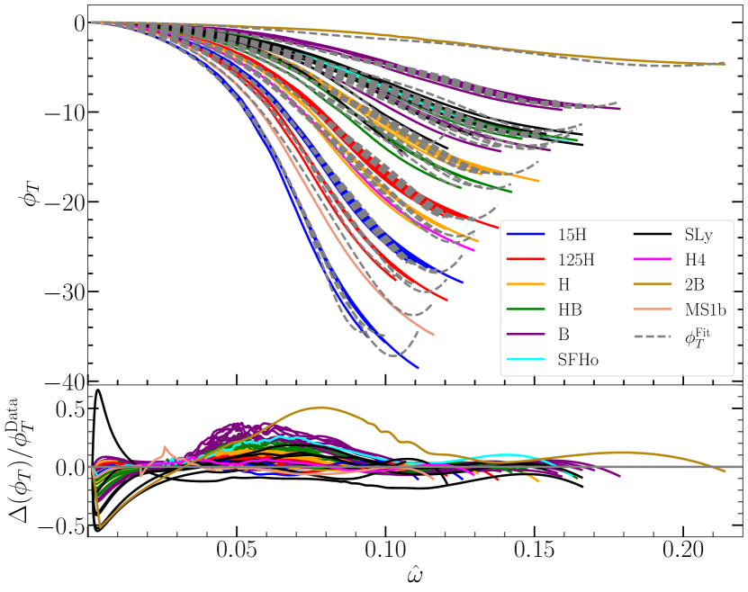
Figure 7: Top: The fits (dashed lines) plotted on top of the time-domain hybridized tidal phase data (solid lines). Bottom: Fractional differences between the fits and the data. The EOB-NR hybrid tidal phases are color-indicated by their EoS.

IV Frequency Domain Representation

IV.1 PN knowledge and SPA

We now construct the frequency-domain phase using Eq. (9) in the stationary phase approximation (SPA) [77, 35]

$$\frac{d^{2}\psi_{T}(\omega)}{d\omega^{2}}=\frac{1}{\omega}\frac{d\phi_{T}(\omega)}{d\omega}.$$ (22)

The 7.5PN order analytical expression [36, 37] of the frequency-domain tidal phase with constant tidal deformability is then

$$\begin{split}\psi_{T}^{\rm PN}=&-\kappa_{A}\bar{c}_{\text{Newt}}^{A}x^{5/2}\Big{(}1+\bar{c}_{1}^{A}x+\bar{c}_{3/2}^{A}x^{3/2}\\ &+\bar{c}_{2}^{A}x^{2}+\bar{c}_{5/2}^{A}x^{5/2}\Big{)}+[A\leftrightarrow B],\end{split}$$ (23)

with

$$\begin{split}\bar{c}_{\text{Newt}}^{A}=&\frac{3(12-11X_{A})(X_{A}+X_{B})^{2}}{16X_{A}X_{B}^{2}},\\ \bar{c}_{1}^{A}=&-5\frac{260X_{A}^{3}-2286X_{A}^{2}-919X_{A}+3179}{672(11X_{A}-12)},\\ \bar{c}_{3/2}^{A}=&-\pi,\\ \bar{c}_{2}^{A}=&\Big{[}5\big{(}4572288X_{A}^{5}-20427120X_{A}^{4}+158378220X_{A}^{3}\\ &+174965616X_{A}^{2}+43246839X_{A}-387973870\big{)}\Big{]}\\ &/[27433728(11X_{A}-12)],\\ \bar{c}_{5/2}^{A}=&-\pi\frac{10520X_{A}^{3}-7598X_{A}^{2}+22415X_{A}-27719}{672(11X_{A}-12)},\end{split}$$ (24)

and similarly for $A\leftrightarrow B$. We use Eq. (23) in constraining the frequency-domain phase for NRTidalv3.

IV.2 Dynamical tides in the frequency domain

One of the main differences between NRTidalv2 and NRTidalv3 is the inclusion of dynamical tides in the latter. Therefore, it is not straightforward to define a constant effective $\kappa_{\text{eff}}$ (as was done in NRTidal [56] and NRTidalv2 [57]) that can be used in both the time- and frequency-domain tidal phases, see also Ref. [60]. We model the entire frequency-domain dynamical tidal deformability (or Love number) in the same manner as in Eq. (12), serving as a frequency-dependent correction/enhancement factor to the adiabatic Love number. This is unlike in Ref. [60], where the frequency-domain dynamical $f$-mode tidal effects were rewritten as an additive correction to the adiabatic component. Hence, we write the PN expression Eq. (23), with $\kappa\rightarrow\kappa(\omega)$ as (for $\ell=2$)

$$\psi_{T,\text{dyn}}^{\rm PN}=\bar{k}_{2}^{\text{eff}}(\hat{\omega})\psi_{T}^{\rm PN}(\hat{\omega}),$$ (25)

where $\bar{k}_{2}^{\text{eff}}(\hat{\omega})$ is the frequency-domain effective tidal enhancement factor. Note that in this case, the same $\bar{k}_{2}^{\rm eff}$ applies to both stars, which makes the calculation of the frequency-domain tidal phase more convenient. We can then solve for $\bar{k}_{2}^{\text{eff}}$ by substituting Eq. (25) into the SPA in Eq. (22), yielding the following differential equation:

$$\frac{d^{2}\bar{k}_{2}^{\text{eff}}}{d\hat{\omega}^{2}}\psi_{T}^{\rm PN}+2\frac{d\bar{k}_{2}^{\text{eff}}}{d\hat{\omega}}\frac{d\psi_{T}^{\rm PN}}{d\hat{\omega}}+\bar{k}_{2}^{\text{eff}}\frac{d^{2}\psi_{T}^{\rm PN}}{d\hat{\omega}^{2}}=\frac{1}{\hat{\omega}}\frac{d\phi_{T,\text{dyn}}^{\rm PN}}{d\hat{\omega}}.$$ (26)

We can then solve for $\bar{k}_{2}^{\text{eff}}$ by imposing the following initial conditions:

$$\bar{k}_{2}^{\text{eff}}(0)=1,\quad\frac{d\bar{k}_{2}^{\text{eff}}(0)}{d\hat{\omega}}=0,$$ (27)

for it to behave similarly to the enhancement factor in the time-domain. Solving for $\bar{k}_{2}^{\text{eff}}$, however, for different values of the tidal parameter and mass can be computationally inefficient, especially when implemented in lalsuite. For this reason, we introduce a phenomenological representation of the enhancement factor of the frequency-domain Love number $\bar{k}_{2,\text{rep}}^{\text{eff}}$ as follows:

$$\begin{split}\bar{k}_{2,\text{rep}}^{\text{eff}}=&1+\frac{s_{1}-1}{\exp[-s_{2}(\hat{\omega}-s_{3})]+1}-\frac{s_{1}-1}{\exp(s_{2}s_{3})+1}\\ &-\frac{s_{2}(s_{1}-1)\exp(s_{2}s_{3})}{[\exp(s_{2}s_{3})+1]^{2}}\hat{\omega},\end{split}$$ (28)

where the parameters $s_{i},\,\,(i=1,2,3)$ are constrained using $s_{i,j},\,\,(j=0,1,2)$:

$$s_{i}=s_{i,0}+s_{i,1}\kappa_{\text{eff}}+s_{i,2}q\kappa_{\text{eff}},$$ (29)

and $\kappa_{\text{eff}}$ is the effective tidal parameter

$$\kappa_{\text{eff}}=\frac{2}{13}\left\{\left[1+\frac{12X_{B}}{X_{A}}\left(\frac{X_{A}}{X_{B}}\right)^{5}k_{2}^{A}\right]+[A\leftrightarrow B]\right\}.$$ (30)

The fitting parameters $s_{i,j}$ for $s_{i}$ are given in Table 2. The fitting formula was chosen to ensure the monotonicity of the enhancement factor $\bar{k}_{2}^{\rm eff}$ up to some maximum at least near (or beyond) the merger frequency, and that it follows the initial conditions laid out in Eq. (27). The fitting formula satisfies the numerically calculated frequency-domain effective enhancement factor, with a maximum (deviation) error of $1.8\%$ and mean error of $0.2\%$.

Table 2: Fitting parameters $s_{i,j}$ for $s_{i}$ that comprise the representation of the frequency-domain Love number enhancement factor, given in Eq. (28).

	0	1	2
$1$	0.273000423	0.00364169971	0.00176144380
$2$	26.8793291	0.0118175396	-0.00539996790
$3$	0.142449682	$-1.70505852\times 10^{-5}$	$3.38040594\times 10^{-5}$

IV.3 NRTidalv3 in the frequency domain

The previously derived representation $\bar{k}_{2,\text{rep}}^{\text{eff}}$ in Eq. (28), which we write from this point onward for convenience as just $\bar{k}_{2}^{\text{eff}}$, can finally be used for building the frequency-domain NRTidalv3 phase:

$$\psi_{T}^{\text{NRT3}}=-\bar{\kappa}_{A}(\hat{\omega})\bar{c}_{\text{Newt}}^{A}x^{5/2}\bar{P}_{\text{NRT3}}^{A}(x)+[A\leftrightarrow B],$$ (31)

where

$$\bar{\kappa}_{A,B}(\hat{\omega})=\kappa_{A,B}\bar{k}_{2}^{\text{eff}}(\hat{\omega}),$$ (32)

$$\begin{split}&\bar{P}_{\text{NRT3}}^{A}(x)\\ &=\frac{1+\bar{n}_{1}^{A}x+\bar{n}_{3/2}^{A}x^{3/2}+\bar{n}_{2}^{A}x^{2}+\bar{n}_{5/2}^{A}x^{5/2}+\bar{n}_{3}^{A}x^{3}}{1+\bar{d}_{1}^{A}x+\bar{d}_{3/2}^{A}x^{3/2}},\end{split}$$ (33)

with

$$\begin{split}\bar{n}_{1}^{A}=&\bar{c}_{1}^{A}+d_{1}^{A},\\ \bar{n}_{3/2}^{A}=&\frac{\bar{c}_{1}^{A}\bar{c}_{3/2}^{A}-\bar{c}_{5/2}^{A}-\bar{c}_{3/2}^{A}\bar{d}_{1}^{A}+\bar{n}_{5/2}^{A}}{\bar{c}_{1}^{A}},\\ \bar{n}_{2}^{A}=&\bar{c}_{2}^{A}+\bar{c}_{1}^{A}\bar{d}_{1}^{A}+\bar{d}_{2}^{A},\\ \bar{d}_{3/2}^{A}=&-\frac{\bar{c}_{5/2}^{A}+\bar{c}_{3/2}^{A}\bar{d}_{1}^{A}-\bar{n}_{5/2}^{A}}{\bar{c}_{1}^{A}}.\end{split}$$ (34)

The remaining parameters are given by

$$\begin{split}\bar{p}_{i}^{A,B}(\hat{\omega})=&\bar{a}_{i,0}+\bar{a}_{i,1}X_{A,B}\\ &+\bar{a}_{i,2}(\kappa_{A,B}+1)^{\bar{\alpha}}\\ &+\bar{a}_{i,3}X_{A,B}^{\bar{\beta}},\,\text{for}\,\bar{p}_{i}\in[\bar{n}_{5/2},\bar{n}_{3}]\\ \bar{d}_{1}^{A,B}=&\bar{d}_{1,0}+\bar{d}_{1,1}X_{A,B}+\bar{d}_{1,2}X_{A,B}^{\bar{\beta}}.\end{split}$$ (35)

The values of the fitting parameters are found in Table 3. For comparison, recently, a phenomenological tidal approximant (with the Padé function up to the $x^{2}$ term in the denominator) was also developed in Ref. [42], where some coefficients of the Padé were constrained to the PN expressions for the tidal and self-spin contributions, while the free coefficients were fitted to the TEOBResumS waveform model; here, two sets of these free coefficents were obtained for $q=1$ and $q>1$. However, for NRTidalv3, we consider the tides to be dynamical, and the free coefficients are themselves explicit functions of the individual masses and/or tidal deformabilities of the system (as indicated in Eq. (35)).

Table 3: Parameters for the NRTidalv3 frequency-domain approximant. The table include the fitting parameters for the dynamical love number enhancement, as well as the respective fitting parameters for the Padé approximant given in Eq. (33).

Tides	$\bar{k}_{2,\text{rep}}^{\text{eff}}$ (Eq. (28))
$\bar{\alpha}$	-0.00808155404
$\bar{\beta}$	-1.13695919
	$\bar{a}_{0}$	$\bar{a}_{1}$	$\bar{a}_{2}$	$\bar{a}_{3}$
$\bar{n}_{5/2}$	-940.654388	626.517157	553.629706	88.4823087
$\bar{n}_{3}$	405.483848	-425.525054	-192.004957	-51.0967553
	$\bar{d}_{1,0}$	$\bar{d}_{1,1}$	$\bar{d}_{1,2}$	-
$d_{1}$	3.80343306	-25.2026996	-3.08054443	-

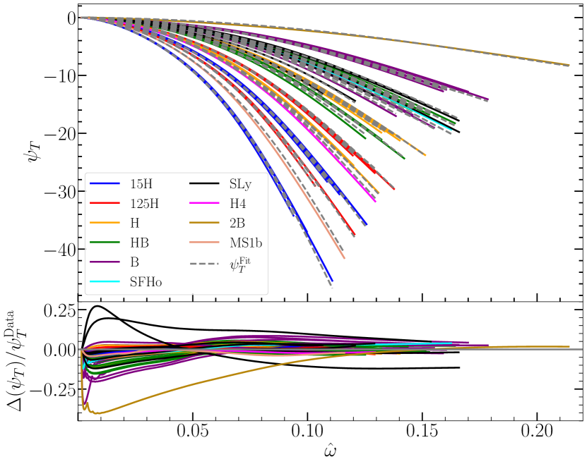
Figure 8: Top: The fits plotted on top of the frequency-domain hybridized tidal phase data. Bottom: Fractional differences between the fits and the data, where $\Delta\psi_{T}=\psi_{T}^{\rm Fit}-\psi_{T}^{\rm Data}$.

We show the results of the fitting in Fig. 8. In this case, the significant fractional differences with respect to the EOB-NR hybrid data $\Delta\psi_{T}^{\rm NRT3}=\Delta\psi_{T}/\psi_{T}^{\rm Data}=(\psi_{T}^{\rm NRT3}-\psi_{T}^{\rm Data})/\psi_{T}^{\rm Data}$ are found again early in the frequencies and around the hybridization window. Furthering the investigation of the performance of NRTidalv3, we plot the difference between the absolute fractional differences of NRTidalv2 and NRTidalv3 with respect to the data, that is, $|\Delta\psi_{T}^{\rm NRT2}|-|\Delta\psi_{T}^{\rm NRT3}|$, against $\hat{\omega}$, and show the results in Fig. 9. We also indicate in the figure $|\Delta\psi_{T}^{\rm NRT2}|-|\Delta\psi_{T}^{\rm NRT3}|=0$, denoted by a black dotted horizontal line. Above this line, NRTidalv2 has greater error with respect to the data than NRTidalv3  and below this line, NRTidalv3 has a greater error. We observe that NRTidalv3 performs overall better than NRTidalv2 for most of the configurations, both for $q=1.0$ (yellow curves) and $q>1.0$ (blue curves).

In addition, we plot the frequency-domain tidal phases of the different NRTidal models for four waveform hybrids in Fig. 10, representing $q=[1.0,1.33,1.75,2.0]$. We note that NRTidalv3 describes the EOB-NR tidal phase contributions better than NRTidalv2 and 7.5PN approximant. We also indicate the merger frequency fit $f_{\rm est}$ from the fitting function shown in Sec. IV.7.

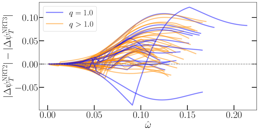
Figure 9: The difference between the absolute fractional differences of NRTidalv3 and NRTidalv2 with respect to the hybrid data. The curves for $q=1.0$ and $q>1.0$ are indicated. We observe NRTidalv3 to perform better (i.e., most curves are above the zero line) than NRTidalv2 for both equal and unequal mass ratios.

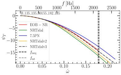
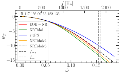
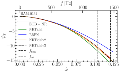
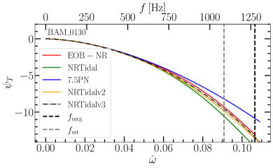
Figure 10: Frequency-domain, EOB-NR hybrid tidal phase contributions of SACRA:B_135_135_00155_182_135, SACRA:B_117_156_00155_182_135, BAM_0131, and BAM_0130, representing mass ratios [1.0, 1.33, 1.75, 2.0]. The tidal phase contributions for NRTidal, NRTidalv2, NRTidalv3, and 7.5PN approximants are also shown. We also indicate the estimated merger frequency $f_{\rm est}$ from the fitting function in Sec. IV.7, and the merger frequency of the NR simulations $f_{\rm mrg}$. The tidal contributions using other tidal models are also shown for comparison.

IV.4 Spin effects

Spinning NS and BH have an infinite series of nonzero multipole moments [78, 79] which will depend on the type of object and its internal structure. Hence, aside from the corrections in the tidal phase contributions that we discussed above, we now include spin effects in NRTidalv3. Here, we follow the same approach as NRTidalv2  where EoS-dependent spin-squared terms up to 3.5PN were included, as well as leading order spin-cubed terms that enter at 3.5PN order [80, 57]. But note that the dynamical-tidal enhancement factor Eq. (12) is specialized to the nonspinning case in this work.

In terms of the spin-induced quadrupolar $C_{\rm Q}^{A,B}$ and octupolar deformabilities $C_{\rm Oc}^{A,B}$ for stars $A$ and $B$, the self-spin terms in the phase that are added to the BBH baseline are given by (for aligned spins)

$$\begin{split}\psi_{\rm SS}=&\frac{3x^{-5/2}}{128\nu}\Bigg{(}\hat{\psi}_{\rm SS,2PN}^{(A)}x^{2}+\hat{\psi}_{\rm SS,3PN}^{(A)}x^{3}+\hat{\psi}_{\rm SS,3.5PN}^{(A)}x^{7/2}\Bigg{)}\\ &+[A\leftrightarrow B],\end{split}$$ (36)

with

$$\begin{split}\hat{\psi}_{\rm SS,2PN}^{(A)}=&-50\hat{C}_{\rm Q}^{A}X_{A}^{2}\chi_{A}^{2},\\ \hat{\psi}_{\rm SS,3PN}^{(A)}=&\frac{5}{84}\left(9407+8218X_{A}-2016X_{A}^{2}\right)\\ &\times\hat{C}_{\rm Q}^{A}X_{A}^{2}\chi_{A}^{2},\\ \hat{\psi}_{\rm SS,3.5PN}^{(A)}=&-400\pi\hat{C}_{\rm Q}^{A}X_{A}^{2}\chi_{A}^{2},\end{split}$$ (37)

where $\hat{C}_{\rm Q}^{A}=C_{\rm Q}^{A}-1$ and $\hat{C}_{\rm Oc}^{A}=C_{\rm Oc}^{A}-1$. We subtract one to remove the BH multipole contribution that is already present in the baseline BBH phase. Meanwhile, the spin-cubed term is given by

$$\begin{split}\psi_{\rm S^{3},3.5PN}^{(A)}=&\frac{3x^{-5/2}}{128\nu}\Bigg{\{}10\Bigg{[}\left(X_{A}^{2}+\frac{308}{3}X_{A}\right)\chi_{A}\\ &+\left(X_{B}^{2}-\frac{89}{3}X_{B}\right)\chi_{B}\Bigg{]}\hat{C}_{\rm Q}^{A}X_{A}^{2}\\ &-440\hat{C}_{\rm Oc}^{A}X_{A}^{3}\chi_{A}^{3}\Bigg{\}}x^{7/2}+[A\leftrightarrow B].\end{split}$$ (38)

To reduce the number of free parameters, we link $C_{\rm Q}^{A}$ to $\Lambda_{A}$, and $C_{\rm Oc}^{A}$ to $C_{\rm Q}^{A}$ via the following EoS-independent relations [81]

$$\begin{split}\log_{10}C_{\rm Q}^{A}=&0.1940+0.09163\log_{10}\Lambda_{A}\\ &+0.04812\log_{10}^{2}\Lambda_{A}-0.004286\log_{10}^{3}\Lambda_{A}\\ &-0.00012450\log_{10}^{4}\Lambda_{A},\end{split}$$ (39)

and

$$\begin{split}\log_{10}C_{\rm Oc}^{A}=&0.003131+2.071\log_{10}C_{\rm Q}^{A}\\ &-0.7152\log_{10}^{2}C_{\rm Q}^{A}+0.2458\log_{10}^{3}C_{\rm Q}^{A}\\ &-0.03309\log_{10}^{4}C_{\rm Q}^{A}.\end{split}$$ (40)

IV.5 Tidal amplitude corrections

We also include amplitude corrections in the NRTidalv3 frequency-domain model following NRTidalv2 [57]. We incorporate these corrections as an ansatz whose form was taken from the frequency-domain representation of TEOBResumS-NR hybrids, as discussed in Ref. [57]:

$$\tilde{A}_{T}^{\rm NRT2}=-\sqrt{\frac{5\pi\nu}{24}}\frac{9M^{2}}{D}\kappa_{\rm eff}x^{13/4}\frac{1+\frac{449}{108}x+\frac{22672}{9}x^{2.89}}{1+13477.8x^{4}},$$ (41)

where $D$ is the luminosity distance to the source.

IV.6 Spin Precession Effects

As with NRTidalv2, we also consider BNS systems whose individual spins have an intrinsic rotation and where this rotation is not necessarily aligned with the orbital angular momentum, causing the orbital plane to precess.

We augment NRTidalv3 onto the BBH baseline IMRPhenomXP, as was done for IMRPhenomXP_NRTidalv2 [82], already available in LALSuite. The IMRPhenomXP baseline improves on IMRPhenomPv2 by incorporating double-spin effects in the twisting-up construction instead of a single-spin approximation. Moreover, the Euler angles are calculated via a precession-averaged treatment of the PN precession dynamics, and there is also an option offered to the user for a more accurate twisting-up prescription based on the solutions of the orbit-averaged SpinTaylorT4 equations implemented in LALSuite. Note that here, the spin-induced multipole corrections introduced in Section IV.4 are applied in the co-precessing frame and then twisted up.

IV.7 Merger Frequency

As a final ingredient for the construction of the full model, we have to define the stopping criterion or the final frequency until which our model is applicable. For this purpose, we use the estimated merger frequency (peak in the GW amplitude) $Mf_{\text{est}}/\nu$ (with $\nu=X_{A}X_{B}=M_{A}M_{B}/M^{2}$) from Ref. [33]. The expression is then given by

$$\frac{Mf_{\text{est}}}{\nu}=w_{0}V^{M}(X),V^{S}(\hat{S},X)V^{T}(\kappa_{2}^{T},X),$$ (42)

where the factor $V^{M}$ depends on the mass ratio, $V^{S}$ depends on the spin contributions (specifically the aligned-spin components of the binary), and $V^{T}$ contains the tidal contributions [33]. The factors are

$$\begin{split}V^{M}=&1+a_{1}^{M}Z,\\ V^{S}=&1+p_{1}^{S}\hat{S},\\ V^{T}=&\frac{1+p_{1}^{T}\kappa_{2}^{T}+p_{2}^{T}(\kappa_{2}^{T})^{2}}{1+p_{3}^{T}\kappa_{2}^{T}+p_{4}^{T}(\kappa_{2}^{T})^{2}},\\ \end{split}$$ (43)

where

$$\begin{split}Z=&1-4\nu,\\ \kappa_{2}^{T}=&3\nu\left[\left(\frac{M_{A}}{M}\right)^{3}\Lambda_{A}+(A\leftrightarrow B)\right],\\ \hat{S}=&\left(\frac{M_{A}}{M}\right)^{2}\chi_{A}+(A\leftrightarrow B),\\ p_{1}^{S}=&a_{1}^{S}(1+b_{1}^{S}Z),\\ p_{i}^{T}=&a_{i}^{T}(1+b_{i}^{T}Z),\end{split}$$ (44)

with coefficients

$$\begin{split}w_{0}=&0.22,\\ a_{1}^{M}=&0.80,\\ a_{1}^{S}=&0.25,\\ a_{i}^{T}\in&[0.0485,5.86\times 10^{-6},0.1,1.86\times 10^{-4}],\\ b_{i}^{T}\in&[1.80,599.99,7.80,84.76].\end{split}$$ (45)

Since the Padé approximant is a rational function, asymptotes (corresponding to a zero denominator in the approximant) can appear depending on the specific source parameters. For this reason, we have performed careful checks to verify that no unphysical behavior occurs, i.e., that the estimated merger frequency of the system (as calculated in Eq. (42)) is less than the frequencies at which the asymptotes occur ($f_{\text{est}}<f_{\text{asymp}}$). Practically speaking, we generated 30,000 random non-spinning configurations with masses $M_{A},\,M_{B}\in[0.5,3.0]$, (corresponding to $X_{A},\,X_{B}\in[0.14,0.86]$) and $\Lambda_{A},\,\Lambda_{B}\in[0,20000]$. We then performed another 30,000 random spinning configurations with aligned-spin components $\chi_{A,B}=[-0.5,0.5]$. For all configurations, we verify that $f_{\text{est}}<f_{\text{asymp}}$ if $f_{\text{asymp}}$ exists. Since NRTidalv3 only models the inspiral part up to the merger of the binary, the condition $f_{\text{est}}<f_{\text{asymp}}$ suffices for the purposes of the model.

However, to ensure that the phase contribution remains smooth even after the merger, i.e., during the time interval when we taper the waveform, and to remove any asymptote, we make the tidal contribution constant if it reaches a local minimum, then connect the tidal phase from inspiral to merger given by $\psi_{T}^{\text{NRT3}}$ and the post-merger with the PN tidal contribution $\psi_{T}^{\rm PN}$(which is polynomial in nature and is therefore smooth) to obtain the tidal function as a function of the frequency:

$$\psi_{T}^{\rm NRT3a}(\hat{\omega})=(1-\sigma(\hat{\omega}))\psi_{T}^{\text{NRT3}}(\hat{\omega})+\sigma(\hat{\omega})\psi_{T}^{\rm PN}(\hat{\omega}),$$ (46)

where $\psi_{T}^{\rm NRT3a}$ includes the post-merger information from PN, and $\sigma(\hat{\omega})$ is the Planck taper:

$$\sigma(\hat{\omega})=\begin{cases}0,\quad&\hat{\omega}\leq\hat{\omega}_{1}\\ \left[1+\exp\left(\frac{\hat{\omega}_{2}-\hat{\omega}_{1}}{\hat{\omega}-\hat{\omega}_{1}}+\frac{\hat{\omega}_{2}-\hat{\omega}_{1}}{\hat{\omega}-\hat{\omega}_{2}}\right)\right]^{-1},\quad&\hat{\omega}_{1}\leq\hat{\omega}\leq\hat{\omega}_{2}\\ 1,\quad&\hat{\omega}\geq\hat{\omega}_{2},\end{cases}$$ (47)

for a frequency window after the estimated merger frequency $[\hat{\omega}_{1},\hat{\omega}_{2}]=[1.15\hat{\omega}_{\text{est}},1.35\hat{\omega}_{\text{est}}]>\hat{\omega}_{\text{est}}=M(2\pi f_{\rm est})$. The same Planck taper is used to taper the entire waveform abruptly up to $1.2\hat{\omega}_{\rm est}$, to minimize the presence of any postmerger signal (since this is not part of the description of NRTidalv3). Then, for the rest of the discussion, we will just refer to the $\psi_{T}^{\rm NRT3a}$ as $\psi_{T}^{\rm NRT3}$, knowing that this implicitly includes the tapered phase beyond merger (in its LALSuite implementation).

V Implementation and Validation

Table 4: Available NRTidal approximants in LAL. The first column contains the BBH baseline model and the second column contains the versions of NRTidal that were added to the BBH model. Full approximant names are given by joining the BBH baseline name with the NRTidal version. We also include information about the corrections in the approximants (i.e., spin-spin, cubic-in-spin, tidal amplitude, and precession), as well as the computational time $\Delta T_{f_{\rm min}}$ of the models at different lower frequencies $f_{\rm min}$. The computational time was obtained using the configuration $M_{A,B}=1.35M_{\odot}$, $\Lambda_{A,B}=400$, with no spins, and were simulated using an Apple M1 Pro processor.

BBH baseline	$\psi_{T}$	Implemented	spin-spin	cubic-in-spin	tidal amp.	precession	$\Delta T_{f_{\rm min}}\,[{\rm s}]$
		by this work?					10 Hz	20 Hz	30 Hz	40 Hz
IMRPhenomD_	NRTidal	No	up to 3PN (BBH)	✗	✗	✗	0.610	0.153	0.038	0.019
	NRTidalv2	No	up to 3PN	✗	✗	✗	1.020	0.253	0.063	0.031
	NRTidalv3	Yes	up to 3PN	✗	✗	✗	2.349	0.591	0.147	0.072
IMRPhenomPv2_	NRTidal	No	up to 3PN	✗	✗	✓	0.745	0.184	0.047	0.023
	NRTidalv2	No	up to 3.5PN	up to 3.5PN	✓	✓	0.969	0.243	0.060	0.030
IMRPhenomXAS_	NRTidalv2	No	up to 3.5PN	up to 3.5PN	✓	✗	0.084	0.022	0.006	0.004
	NRTidalv3	Yes	up to 3.5PN	up to 3.5PN	✓	✗	0.089	0.026	0.008	0.005
IMRPhenomXP_	NRTidalv2	No	up to 3.5PN	up to 3.5PN	✓	✓	0.353	0.091	0.024	0.013
	NRTidalv3	Yes	up to 3.5PN	up to 3.5PN	✓	✓	0.358	0.093	0.025	0.014
SEOBNRv4_ROM_	NRTidal	No	up to 3PN	✗	✗	✗	0.423	0.110	0.029	0.016
	NRTidalv2	No	up to 3.5PN	up to 3.5PN	✓	✗	0.630	0.163	0.043	0.022
SEOBNRv5_ROM_	NRTidal	Yes	up to 3PN	✗	✗	✗	0.418	0.102	0.030	0.017
	NRTidalv2	Yes	up to 3.5PN	up to 3.5PN	✓	✗	0.639	0.168	0.045	0.024
	NRTidalv3	Yes	up to 3.5PN	up to 3.5PN	✓	✗	1.193	0.306	0.080	0.041

To make use of the newly developed NRTidalv3 model, we implement it into LALSuite [58] by adding the outlined corrections to several different BBH baseline models: the spinning, non-precessing models IMRPhenomD [83], IMRPhenomXAS [84], SEOBNRv5_ROM [85], and the spinning, precessing model IMRPhenomXP [86]. We list all the new approximants in Table 4. The full approximant name is given by combining the BBH baseline name with the NRTidal version (e.g., IMRPhenomXAS_NRTidalv3). Versions of NRTidal which are currently present in LALSuite are shown in Table 4, both previously existing models and the ones newly implemented in this work. We also show in Table 4 their computation times employing different values of starting frequencies and using a sampling rate of $2^{15}=32768$ Hz, for a system $M_{A}=M_{B}=1.35M_{\odot}$ and $\Lambda_{A}=\Lambda_{B}=400$. Overall, we find that NRTidalv3 has retained both speed and efficiency (particularly for starting frequencies $f_{\rm min}\geq 20\,{\rm Hz}$) despite having a more accurate (and mathematically more complicated) description of the GW signal than NRTidalv2.

Table 5: BNS configurations for the time-domain dephasing comparisons. We show the configurations of NR simulations using BAM, SACRA, and SpEC that are used in the comparison of waveforms in the time domain. The SACRA waveforms, as well as BAM:0001, BAM:0037 and BAM:0064, are also used in the calibration in NRTidalv3. For each NR simulation listed here, we indicated the EOS used, the individual masses $M_{A,B}$, spins $\chi_{A,B}$, tidal deformabilities $\Lambda_{A,B}$, effective tidal deformability $\tilde{\Lambda}$ of the system, resolution $h_{\rm fine}$, eccentricity $e$, and whether or not a Richardson extrapolated waveform was constructed from the simulations.

Name	EOS	$M_{A}$ [$M_{\odot}$]	$M_{B}$ [$M_{\odot}$]	$\chi_{A}$	$\chi_{B}$	$\Lambda_{A}$	$\Lambda_{B}$	$\tilde{\Lambda}$	$h_{\text{fine}}$[$M_{\odot}$]	$e\ [10^{-3}]$	Richardson
CoRe:BAM:0001	2B	1.35	1.35	0	0	126.7	126.7	126.7	0.093	7.1	✗
CoRe:BAM:0011	ALF2	1.5	1.5	0	0	382.8	382.8	382.8	0.125	3.1	✗
CoRe:BAM:0037	H4	1.37	1.37	0	0	1006.2	1006.2	1006.2	0.0833	0.9	✓
CoRe:BAM:0039	H4	1.37	1.37	0.141	0.141	1001.8	1001.8	1001.8	0.0833	0.5	✓
CoRe:BAM:0062	MS1b	1.35	1.35	-0.099	-0.099	1531.5	1531.5	1531.5	0.097	1.8	✓
CoRe:BAM:0068	MS1b	1.35	1.35	0.149	0.149	1525.2	1525.2	1525.2	0.097	2.2	✓
CoRe:BAM:0081	MS1b	1.5	1.00	0	0	863.8	7022.4	2425.5	0.125	15.5	✗
CoRe:BAM:0094	MS1b	1.94	0.944	0	0	182.9	9279.9	1308.2	0.125	3.3	✗
SACRA:15H_135_135	15H	1.35	1.35	0	0	1211	1211	1211	0.0508	$\lesssim 1$	✗
_00155_182_135
SACRA:HB_121_151	HB	1.21	1.51	0	0	200	827	422	0.0555	$\lesssim 1$	✗
_00155_182_135
SXS:NSNS:001	$\Gamma 2$	1.40	1.40	0	0	791	791	791	0.133	$\sim 2$	✗
SXS:NSNS:002	MS1b	1.35	1.35	0	0	1540	1540	1540	0.159	$\sim 2$	✗

V.1 Time Domain Comparisons

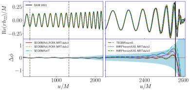
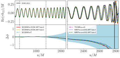
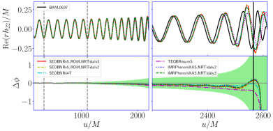
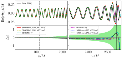
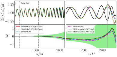
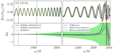
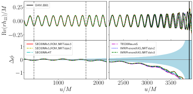
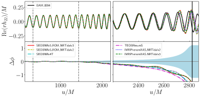
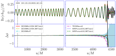
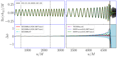
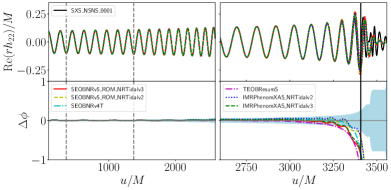
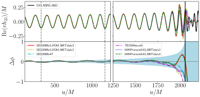
Figure 11: Time-domain dephasing comparisons for the BAM, SACRA, and SpEC waveforms. For each NR waveform, the upper panel shows the real part of the gravitational wave strain as a function of the retarded time, while the bottom panel shows the phase difference between the waveform model and the NR waveform. We note that BAM:0001, BAM:0037, and both SACRA waveforms (indicated by blue frames in their plots) were also used in the calibration of NRTidalv3.

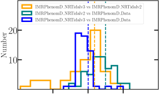
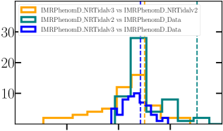
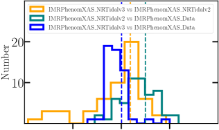
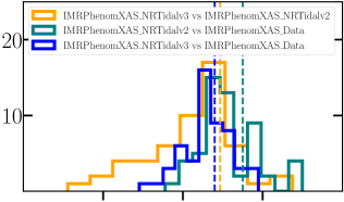
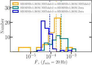
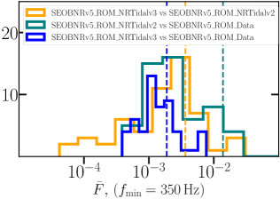
Figure 12: Mismatch histograms for different BBH baselines augmented with the NRTidalv3 model, versus the BBH baseline model added with the EOB-NR hybrid tidal phase. Vertical lines denote the mean of the histograms with the same color. The mismatches with NRTidalv2 are also shown for comparison. For each BBH baseline + NRTidalv3 model, mismatches are computed starting from $f_{\rm min}=20\,{\rm Hz}$ in the left panel, indicating the mismatch for the full waveform where EOB contribution is present in the early inspiral. Mismatches are also computed for $f_{\rm min}=350\,{\rm Hz}$ in the right panel, where typically the hybridization starts and where the NR contribution becomes dominant up to merger.

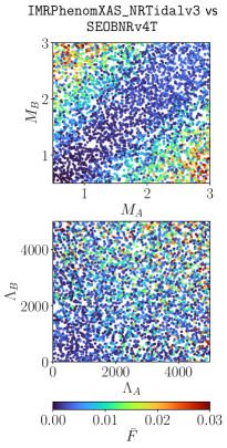
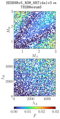
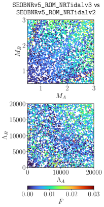
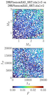
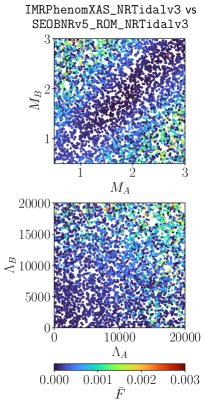
Figure 13: Mismatch Comparisons of NRTidalv3 with other tidal waveform models for non-spinning configurations. Each comparison with either TEOBResumS or SEOBNRv4T  contains 4000 random configurations of mass $M_{A,B}=[0.5,3.0]$ and tidal deformability $\Lambda_{A,B}=[0,5000]$. The rest of the comparisons are done with $\Lambda_{A,B}=20000$. For each subfigure we include a color bar indicating the values of the mismatches. Note that the maximum value in the color bar for IMRPhenomXAS_NRTidalv3 vs SEOBNRv5_ROM_NRTidalv3 is different from the rest of the subfigures due to the NRTidalv3 models yielding very small mismatches with respect to each other.

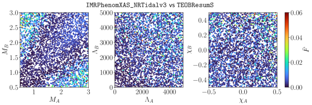
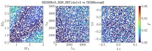
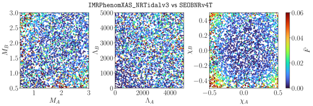
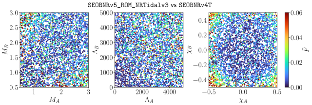
Figure 14: Mismatch Comparisons of NRTidalv3 with other tidal waveform models for aligned-spin configurations. Each subfigure has 4000 random configurations of mass $M_{A,B}=[1.0,3.0]$, tidal deformability $\Lambda_{A,B}=[0,5000]$ and spin $\chi_{A,B}=[-0.5,0.5]$. We also put the mismatches with NRTidalv2 for comparison. For each subfigure we include a color bar indicating the values of the mismatches.

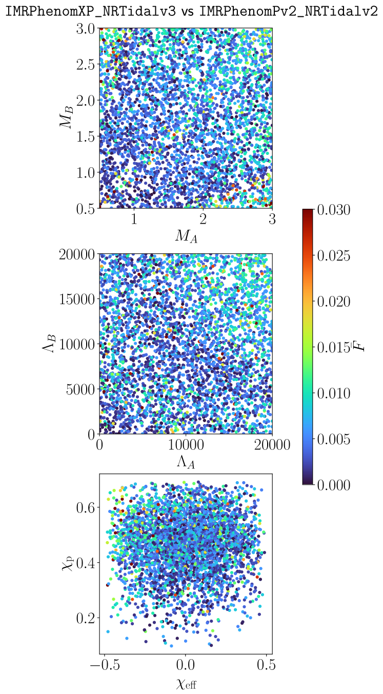
Figure 15: Mismatches for IMRPhenomXP_NRTidalv3 vs IMRPhenomPv2_NRTidalv2 for precessing configurations. For this comparison, we generate 4000 random samples with mass $M_{A,B}=[0.5,3.0]$, tidal deformabilities $\Lambda_{A,B}=[0,20000]$, and spins $\chi_{A,B,C}^{x,y,z}=[-0.5,0.5]$. For the spins, we plot the effective spin precession $\chi_{p}$ against the effective aligned spin $\chi_{\rm eff}$. We include a colorbar indicating the values of the mismatches.

In this section, we compare the waveform models utilizing NRTidalv3 with other waveforms, particularly their corresponding NRTidalv2 versions, as well as the SEOBNRv4T model using NR waveforms from BAM [31, 33], SACRA [69, 28, 29], and SpEC [30]. The configurations of the NR waveforms used for comparison are found in Table 5. We note that the waveforms named BAM:0001, BAM:0037, SACRA:15H_135_135_00155_182_135, and SACRA:HB_121_151_00155_182_135 are also used in the calibration of NRTidalv3 (see Table 7 in Appendix A). For NRTidalv3 we employ IMRPhenomXAS_NRTidalv3  and SEOBNRv5_ROM_NRTidalv3, and the other tidal waveforms for the comparison are TEOBResumS [87, 88, 46, 89, 90, 91], SEOBNRv4T [49], SEOBNRv5_ROM_NRTidalv2 (also implemented by this work), and IMRPhenomXAS_NRTidalv2.

For the time-domain comparison, we are first aligning the waveforms using the same procedure as for the construction of the EOB-NR hybrids described in Sec. II. Fig. 11 shows our comparison for the BAM waveforms, where we also indicate the numerical uncertainty as shaded bands. In particular, we use a blue band for setups for which we just calculate the phase difference between the two highest resolutions . For NR simulations where we find a clear convergence order and employ the Richardson-extrapolated waveform, we are using a green band as an error measure given by the phase difference between the Richardson-extrapolated waveform and the highest resolution.

We observe from Fig. 11 that for the BAM NR data, both NRTidalv3 models perform well in terms of the dephasing with respect to the NR waveforms, and the NRTidalv3 models are consistent with the other models such that they generally fall within the estimated numerical uncertainties. The exception to this would be for BAM:0081 and BAM:0094 (the same can be said for the other waveform models), which are characterized by large mass ratios, and large tidal deformabilities which are far outside the space of calibration for NRTidalv3, though we still observe NRTidalv3 to perform a bit better than NRTidalv2. We also note that the employed EoS for these setups (MS1b) is already disfavored by the observation of GW170817 [2, 3, 4], i.e., this could be considered as a reasonable upper bound for a realistic BNS setup. We also present the comparison between the models and the SACRA and SpEC waveforms. Generally, due to the higher resolution, the computed uncertainties are generally smaller than for the BAM waveforms, however, we do not see a clear convergence order, which means that we cannot estimate the error based on Richardson extrapolation. For SACRA waveforms, we see that the NRTidalv3 models perform better than the other waveform models. However, we note that this might also simply be due to the fact that the same waveforms were also used in the calibration of NRTidalv3. Meanwhile, no model was able to capture the merger part of SXS:NSNS:0001, while NRTidalv3 performed better than the others in terms of the dephasing for SXS:NSNS:002.

V.2 Mismatch against EOB-NR hybrid data

We further test the accuracy of our fits by comparing mismatches of the NRTidalv2 and NRTidalv3 models with the hybrid EOB-NR waveforms. The mismatch (or unfaithfulness) between two frequency-domain complex waveforms $\tilde{h}_{1}$ and $\tilde{h}_{2}$ is given by

$$\bar{F}=1-\text{max}_{\phi_{c},t_{c}}\frac{(h_{1}(\phi_{c},t_{c})|h_{2})}{\sqrt{(h_{1}|h_{1})(h_{2}|h_{2})}},$$ (48)

where the overlap is

$$(h_{1}|h_{2})=4{\rm Re}\int_{f_{\text{min}}}^{f_{\text{max}}}\frac{\tilde{h}_{1}^{*}(f)\tilde{h}_{2}(f)}{S_{n}(f)}df,$$ (49)

and the maximization of the overlap for some arbitrary phase $\phi_{c}$ and time shift $t_{c}$ (in the time domain, corresponding to a phase and frequency shift in the frequency domain) ensures the alignment between the two waveforms. Here, we assume the spectral density of the detector as $S_{n}(f)=1.0$ so that the computation is detector-agnostic. We set $f_{\text{max}}=f_{\text{mrg}}$. For the waveforms, we choose a sampling rate of $2^{13}=8192$ Hz. For a full comparison, we construct full waveforms with corresponding BBH baselines (from the model we want to compare with) and add to its phase the EOB-NR hybrid tidal phase, i.e., we have IMRPhenomD_Data, IMRPhenomXAS_Data, and SEOBNRv5_ROM_Data. The minimum frequency $f_{\text{min}}$ is chosen to be either 20 Hz or 350 Hz. The former takes into account almost the entire hybrid waveform, which is dominated in the very early inspiral by the EOB model used for constructing the EOB-NR hybrid (SEOBNRv4T), while the latter value considers mainly the NR contribution (typically where the hybridization starts).

We show results as mismatch histograms for IMRPhenomD_NRTidalv3, IMRPhenomXAS_NRTidalv3, and SEOBNRv5_ROM_NRTidalv3 in Fig. 12. Taking a look, for example, at the histograms for IMRPhenomD_NRTidalv3 with $f_{\rm min}=20\,{\rm Hz}$ (the uppermost left panel), we compute the mismatches between IMRPhenomD_NRTidalv3 and IMRPhenomD_Data, between IMRPhenomD_NRTidalv3 and IMRPhenomD_NRTidalv2, and between IMRPhenomD_NRTidalv2 and IMRPhenomD_Data. For each histogram, the mean mismatch $\mu_{\bar{F}}$ is indicated by a vertical dashed line. The mismatches are larger with larger $f_{\rm min}$. We note the improvement in the accuracy of the NRTidalv3 waveforms with respect to NRTidalv2, as indicated by their lower mismatches with respect to the hybrid data. In general, NRTidalv3 has a mismatch of about half of an order of magnitude smaller than that of NRTidalv2. We also note that for $f_{\rm min}=350\,{\rm Hz}$, NRTidalv2 has a tail in its distribution for $\bar{F}\gtrsim\mathcal{O}(10^{-2})$, while this is not present for NRTidalv3. While the reduction of the mismatch is to some extent also caused by the fact that all of the employed waveforms have been used in the calibration of NRTidalv3, it still shows the overall robustness and performance of the model.

Table 6: The mean mismatch $\mu_{\bar{F}}$ and maximum mismatch ${\rm max}(\bar{F})$ for various waveform model comparisons for the non-spinning, aligned-spin, and precessing configurations. A ‘$-$’ symbol indicates that the mismatches were not calculated between the two waveform models.

Non-Spinning Case
		IMRPhenomXAS_NRTidalv3	SEOBNRv5_ROM_NRTidalv3
IMRPhenomXAS_NRTidalv3	$\mu_{\bar{F}}$	$-$	$3.608\times 10^{-4}$
	${\rm max}(\bar{F})$	$-$	0.005032
SEOBNRv5_ROM_NRTidalv3	$\mu_{\bar{F}}$	$3.608\times 10^{-4}$	$-$
	${\rm max}(\bar{F})$	0.005032	$-$
TEOBResumS	$\mu_{\bar{F}}$	0.004238	0.004736
	${\rm max}(\bar{F})$	0.02527	0.02648
IMRPhenomXAS_NRTidalv2	$\mu_{\bar{F}}$	0.004279	$-$
	${\rm max}(\bar{F})$	0.02804	$-$
SEOBNRv5_ROM_NRTidalv2	$\mu_{\bar{F}}$	$-$	0.006038
	${\rm max}(\bar{F})$	$-$	0.03243
SEOBNRv4T	$\mu_{\bar{F}}$	0.005874	0.006729
	${\rm max}(\bar{F})$	0.03282	0.03415
Aligned Spin Case
		TEOBResumS	SEOBNRv4T
IMRPhenomXAS_NRTidalv3	$\mu_{\bar{F}}$	0.005577	0.01456
	${\rm max}(\bar{F})$	0.06703	0.1713
SEOBNRv5_ROM_NRTidalv3	$\mu_{\bar{F}}$	0.006278	0.01454
	${\rm max}(\bar{F})$	0.06221	0.1708
Precessing Case
		IMRPhenomXP_NRTidalv3	$-$
IMRPhenomPv2_NRTidalv2	$\mu_{\bar{F}}$	0.0056560	$-$
	${\rm max}(\bar{F})$	0.08585	$-$

V.3 Mismatches against other tidal waveform models

Finally, we want to compare our model with other tidal models in three cases: (a) non-spinning configurations, (b) aligned spins, and (c) precessing systems. For the non-spinning configurations, we compute the mismatch between NRTidalv3 (specifically, IMRPhenomXAS_NRTidalv3 and SEOBNRv5_ROM_NRTidalv3) and TEOBResumS, SEOBNRv4T, and NRTidalv2. The mismatches computed in this section assume $f_{\rm min}=40\,{\rm Hz}$, $f_{\rm max}=2048\,{\rm Hz}$ and a waveform sampling rate of $2^{13}=8192\,{\rm Hz}$, except for when comparisons are done with SEOBNRv4T, where a sampling rate of $2^{13}=4096\,{\rm Hz}$ was used for the sake of efficiency.

Non-spinning setups:

In the non-spinning case, the mismatches are computed for 4000 random configurations of masses $M_{A,B}=[0.5,3.0]M_{\odot}$ and tidal deformabilities $\Lambda_{A,B}=[0,5000]$, for comparisons done with TEOBResumS and SEOBNRv4T. For $\Lambda_{A,B}\geq 5000$, and especially when combined with a high-mass-ratio or high-spin configuration, we find both TEOBResumS and SEOBNRv4T to fail to produce a waveform. For comparisons which do not involve these two waveform models, we use $\Lambda_{A,B}=[0,20000]$. These mismatches are then plotted in a 2D scatter plot (in the x-y plane) with the masses and tidal deformabilites (Fig. 13). In addition, we also directly compare the mismatches between the NRTidalv3 models. We note the very small mismatches, with $\mu_{\tilde{F}}=3.608\times 10^{-4}$, indicating that the waveforms behave very similarly to each other. In general, we find very small mismatches for relatively low masses and low-mass ratios, with the largest mismatches occurring at higher masses ($M_{A,B}\gtrsim 2.0M_{\odot}$) and high mass-ratios ($q\gtrsim 1.5$). Large mismatches also occur for large tidal deformabilities ($\Lambda_{A,B}\gtrsim\mathcal{O}(10^{3})$). For all comparisons in the non-spinning case (except IMRPhenomXAS_NRTidalv3 vs SEOBNRv5_ROM_NRTidalv3) $\mu_{\bar{F}}=\mathcal{O}(10^{-3})$ and ${\rm max}(\bar{F})=\mathcal{O}(10^{-2})$ (see Table 6 ).

Aligned-spin setups:

For the aligned-spin configurations, we compute the mismatches between two NRTidalv3 variants, IMRPhenomXAS_NRTidalv3 and SEOBNRv5_ROM_NRTidalv3  and these NRTidalv3 variants against TEOBResumS and SEOBNRv4T. In addition to the 4000 random configurations of the masses and tidal deformabilities used in the non-spinning case, that we generated for the non-spinning case, we also generate 4000 random aligned spins $\chi_{A,B}=[-0.5,0.5]$. In the mismatch scatter plots, we plot the masses, the tidal deformabilities, and the aligned-spin components in the $x-y$ plane, and the mismatches in the color bar (see Fig. 14). When the NRTidalv3 variants are compared against TEOBResumS, large tidal deformabilities ($\Lambda=\mathcal{O}(10^{3})$), mass-ratios ($q\gtrsim 1.5$), and masses ($M_{A,B}\gtrsim 2.0$) result to large mismatches. In general, comparisons with SEOBNRv4T yield on average larger mismatches than that with TEOBResumS (see Table 6). The mismatches are largest ($\mathcal{O}(10^{-1})$) for the configurations with very high spin magnitudes $|\chi_{A,B}|\gtrsim 0.4$.

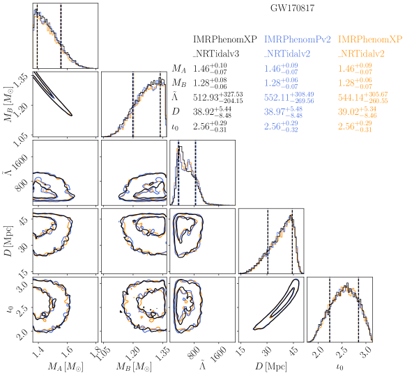
Figure 16: The marginalized 1D and 2D posterior probability distributions for selected parameters of GW170817, obtained with IMRPhenomXP_NRTidalv3 (black), IMRPhenomPv2_NRTidalv2 (blue), and IMRPhenomXP_NRTidalv2 (orange). The parameters shown here are the individual star masses $M_{A,B}$, binary tidal deformability $\tilde{\Lambda}$, luminosity distance $D$, and inclination angle $\iota_{0}$. The 68% and 90% confidence intervals are indicated by contours for the 2D posterior plots, while vertical lines in the 1D plots indicate 90% confidence interval. We note a narrow constraint on the tidal deformability for IMRPhenomXP_NRTidalv3 compared to the other models, due to the updated tidal information that was used.

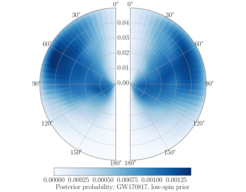
Figure 17: Inferred spin parameters for GW170817 from a low-spin prior ($\chi\leq 0.05$) using IMRPhenomXP_NRTidalv3. Plotted here are the probability densities for the dimensionless spin components $\chi_{1}$ (left hemisphere) and $\chi_{2}$ (right hemisphere) relative to the orbital angular momentum $\mathbf{L}$ and tilt angles (a tilt angle $0^{\circ}$ means that the spin is aligned with the $\mathbf{L}$). The plot was done using a reference frequency of 20 Hz.

Precessing setups:

For the precessing configurations, we compare IMRPhenomXP_NRTidalv3 and IMRPhenomPv2_NRTidalv2 [92, 57]. Aside from the randomly generated masses and tidal deformabilities used in the non-spinning and aligned-spin cases, we also generate 4000 random values of the $x,y,z$ components of the spin, $\chi_{A,B}^{x,y,z}=[-0.5,0.5]$. Here, for the spins, we plot in Fig. 15 on the $x-y$ plane the effective spin precession $\chi_{p}$ against the effective aligned spin $\chi_{\rm eff}$, where

$$\chi_{p}=\frac{S_{p}}{K_{A}M_{A}^{2}},$$ (50)

where $S_{p}$ is the average magnitude of the spins:

$$S_{p}={\rm max}(K_{A}S_{A,\perp},K_{B}S_{B,\perp}),$$ (51)

with $K_{A}=2+3/(2q)$ (with $M_{A}>M_{B}$), and $S_{A,\perp}$ is the magnitude of the in-plane spin for body $A$ [93]. Meanwhile, the effective aligned spin is given by

$$\chi_{\rm eff}=\mathbf{m}_{A}\chi_{A}+\mathbf{m}_{B}\chi_{B},$$ (52)

where $\mathbf{m}_{A,B}=(1/2)(1\pm\sqrt{1-4\nu})$. From Fig. 15, we observe large mismatches ($\mathcal{O}(10^{-2})$) for configurations with large masses ($M_{A,B}\gtrsim 2.5M_{\odot}$), large tidal deformabilities ($\Lambda_{A,B}\gtrsim\mathcal{O}(10^{3})$), or large $\chi_{p}$ and $|\chi_{\rm eff}|$ ($\gtrsim 0.4$).

For all the configurations discussed above, we calculate the mean mismatch $\mu_{\bar{F}}$ and maximum mismatch ${\rm max}(\bar{F}$) for all waveform comparisons done. The results are shown in Table 6.

VI Parameter Estimation

Finally, to test the applicability of the developed NRTidalv3 models, we will reanalyze the two BNS detections GW170817 [2] and GW190425 [5]. For this purpose, we utilize parallel bilby [94, 95], which performs GW parameter estimation using a parallelized nested sampler named dynesty [96]. Parallel bilby uses Bayes’ theorem:

$$P(\theta|d,\mathcal{H})=\frac{\mathcal{L}(d|\theta,\mathcal{H})p(\theta|\mathcal{H})}{E(d|\mathcal{H})},$$ (53)

where $P(\theta|d,\mathcal{H})$ is the posterior probability distribution of the parameters $\theta$ given some data $d$ (which consists the waveform) and hypothesis $\mathcal{H}$, $p(\theta|\mathcal{H})$ is the prior probability distribution, and $E(d|\mathcal{H})$ is the evidence, serving as normalization constant to $P(\theta|d,\mathcal{H})$. Meanwhile, $\mathcal{L}(d|\theta,\mathcal{H})$ is the likelihood of obtaining the data $d$ given that the parameters $\theta$ are under the hypothesis $\mathcal{H}$. For further details, we refer to Refs. [94, 97, 98]. In our study, we use GW170817 and GW190425 as our GW events, and we use the following waveform models: IMRPhenomXP_NRTidalv3, IMRPhenomPv2_NRTidalv2, and IMRPhenomXP_NRTidalv2, and also compare their results with each other. We also use low-spin and high-spin priors for both GW events following the standard LIGO Scientific-, Virgo, KAGRA Collaboration (LVK) analyses [23, 2, 97, 10, 5, 98].

VI.1 GW170817

We show the results of the inferred marginalized 1D and 2D posterior probability distribution of a selection of source parameters for GW170817 in Fig. 16, for a low-spin prior with $\chi\leq 0.05$. In this figure, we show the individual masses of the stars $M_{A,B}$, the luminosity distance $D$ in Mpc, and the inclination angle $\iota_{0}$. We also include here dimensionless tidal deformability defined in terms of the individual masses and tidal deformabilities of the stars [10]:

$$\tilde{\Lambda}=\frac{16}{13}\frac{(M_{A}+12M_{B})M_{A}^{4}\Lambda_{A}+(M_{B}+12M_{A})M_{B}^{4}\Lambda_{B}}{(M_{A}+M_{B})^{5}}.$$ (54)

From Fig. 16, we note that the performance of IMRPhenomXP_NRTidalv3 in terms of the inferred parameters is consistent with the results of IMRPhenomPv2_NRTidalv2 [23]. The main difference is the slightly tighter constraint of IMRPhenomXP_NRTidalv3 for $\tilde{\Lambda}$ compared to the other models (which are based on NRTidalv2). This is due to the reduction of the secondary peak that NRTidalv2 models show at higher $\tilde{\Lambda}$.

Finally, we investigate the spin constraints of IMRPhenomXP_NRTidalv3 on GW170817 by plotting the inferred spin component magnitudes and orientation (in terms of tilt angles). A tilt angle of $0^{\circ}$ means that the spin components are aligned with the orbital angular momentum $\mathbf{L}$. The results are shown in Fig. 17, where the left hemisphere is for $\chi_{1}$ and the right hemisphere corresponds to $\chi_{2}$. We note that large negative components and anti-aligned spins are ruled out, which is consistent with previous studies using IMRPhenomPv2_NRTidalv2 [23].

For the corresponding parameter estimation for the high-spin prior ($\chi\leq 0.5$), we refer to Appendix B.

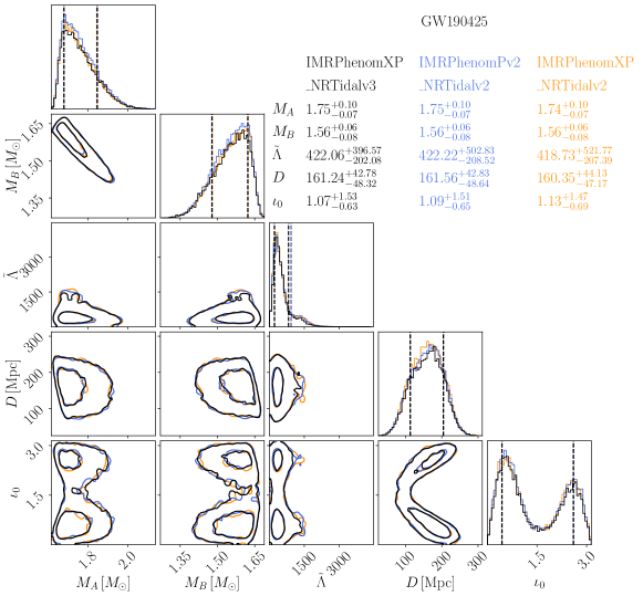
Figure 18: The marginalized 1D and 2D posterior probability distributions for selected parameters of GW190425, obtained with IMRPhenomXP_NRTidalv3 (black), IMRPhenomPv2_NRTidalv2 (blue), and IMRPhenomXP_NRTidalv2 (orange). The parameters shown here are the individual star masses $M_{A,B}$, binary tidal deformability $\tilde{\Lambda}$, luminosity distance $D$, and inclination angle $\iota_{0}$. The 68% and 90% confidence intervals are indicated by contours for the 2D posterior plots, while vertical lines in the 1D plots indicate 90% confidence interval. As with GW170817, note a narrow constraint on the tidal deformability for IMRPhenomXP_NRTidalv3 compared to the other models, due to the updated tidal information that was used.

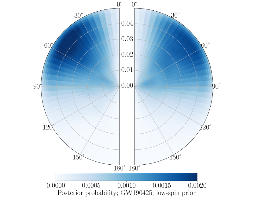
Figure 19: Inferred spin parameters for GW190425 from a low-spin prior ($\chi\leq 0.05$) using IMRPhenomXP_NRTidalv3. Plotted here are the probability densities for the dimensionless spin components $\chi_{1}$ (left hemisphere) and $\chi_{2}$ (right hemisphere) relative to the orbital angular momentum $\mathbf{L}$ and tilt angles (i.e. a tilt angle $0^{\circ}$ means that the spin is aligned with the $\mathbf{L}$). The plot was done at a reference frequency of 20 Hz.

VI.2 GW190425

The results for the marginalized posterior distributions for GW190425 can be found in Fig. 18, where (as in the case for GW170817), we see a slightly tighter constraint on the tidal deformability $\tilde{\Lambda}$ from IMRPhenomXP_NRTidalv3, than the other waveform models. However, all results are consistent between the different GW models.

Finally, the spin magnitudes and orientation inferred for GW190425 using IMRPhenomXP_NRTidalv3 in Fig. 19 shows that negative values of the spin component magnitudes are heavily disfavored, as well as orientation greater than $90^{\circ}$. The corresponding parameter estimation for the high-spin prior ($\chi\leq 0.5$) is found in Appendix B.

VI.3 Performance of NRTidalv3

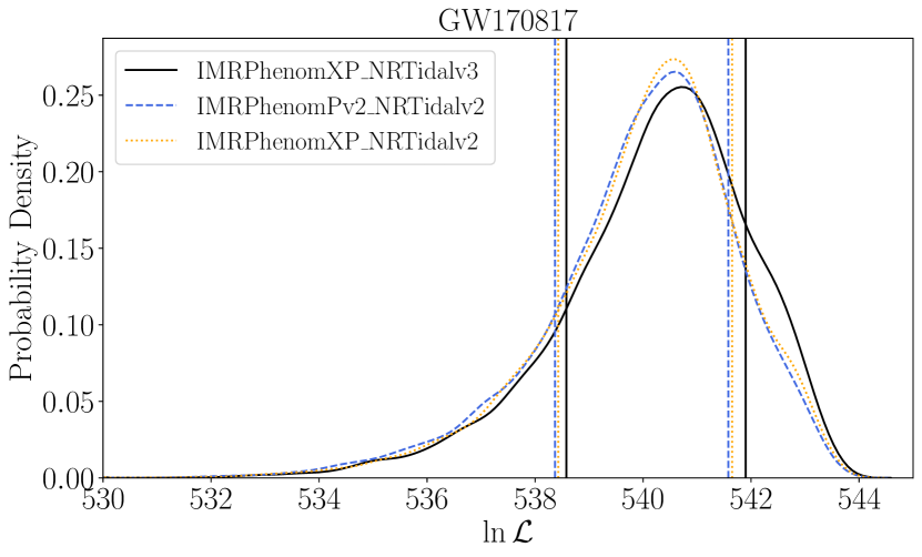
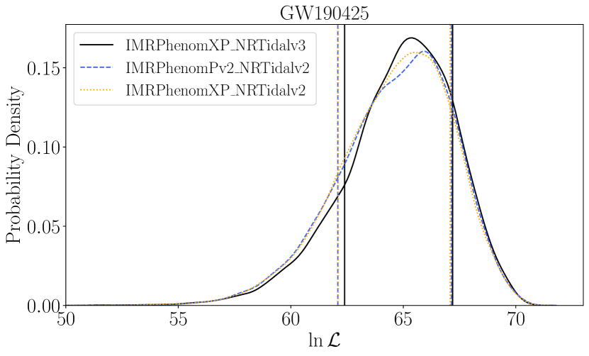
Figure 20: The distribution of the log-likelihood $\ln\mathcal{L}$ for GW170817 (top) and GW190425 (bottom). The vertical lines indicate 90% confidence intervals for the models. We note the shifting of the distribution using IMRPhenomXP_NRTidalv3 towards larger $\ln\mathcal{L}$.

To further investigate the performance of IMRPhenomXP_NRTidalv3  we plot the posterior probability distribution of the natural logarithm of its likelihood (also known as the log-likelihood), $\ln\mathcal{L}$, and compare it with the other two waveform models, as shown in the top panel of Fig. 20. We note that for GW170817, the $\ln\mathcal{L}$ of IMRPhenomXP_NRTidalv3 is generally shifted towards slightly larger values when compared to that of IMRPhenomPv2_NRTidalv2 and IMRPhenomXP_NRTidalv2. In addition, we compute the Bayes factors (which is the ratio of the evidences or posterior probabilities) with respect to the null hypothesis of a non-detection and find IMRPhenomXP_NRTidalv3 has $\ln\mathcal{B}=526.726\pm 0.085$ which is larger than that of IMRPhenomPv2_NRTidalv2 ($\ln\mathcal{B}=526.647\pm 0.084$) and IMRPhenomXP_NRTidalv2 ($\ln\mathcal{B}=526.668\pm 0.079$). Although these numbers might indicate a slight preference for IMRPhenomXP_NRTidalv3, they are not statistically significant.

Similar to GW170817, we also present the log-likelihood for GW190425 in the bottom panel of Fig. 20. As before, we find slightly larger $\ln\mathcal{L}$ for IMRPhenomXP_NRTidalv3, and at the same time Bayes Factors of IMRPhenomXP_NRTidalv3  $\ln\mathcal{B}=53.849\pm 0.079$, which is larger than that of IMRPhenomPv2_NRTidalv2 ($\ln\mathcal{B}=53.756\pm 0.079$) and IMRPhenomXP_NRTidalv2 ($\ln\mathcal{B}=53.766\pm 0.079$), though with overlapping uncertainties and not being statistically significant.

VII Conclusions and Outlook

Summary:

In this work, we introduced NRTidalv3 as a new description of the tidal phase contribution to the total GW phase of BNS systems. This model improves upon the previous version (NRTidalv2) by employing a larger set of NR waveforms across a wide range of tidal deformabilities with mass ratios up to $q=2.0$. To construct the model, we employed a representation of the frequency-domain, dynamical enhancement factor for the Love number, as well as a Padé approximant, which imposes additional constraints pertaining to the masses and tidal deformabilities of the component stars.

The model was then augmented onto existing BBH baseline models in LALSuite (IMRPhenomD, IMRPhenomXAS, IMRPhenomXP, and SEOBNRv5_ROM). To test the performance of NRTidalv3  we calculated its dephasing relative to existing NR waveforms and found overall consistency between NRTidalv3 with respect to the uncertainties in the NR waveforms and with respect to other waveform models. The computed mismatches between NRTidalv3 and NR waveforms, as well as NR hybrids, were smaller than for the previously constructed model NRTidalv2 [57]. With respect to other tidal waveform models, we observe the largest mismatches for high masses, mass ratios, tidal deformabilities, and spin magnitudes. However, we find that overall NRTidalv3 can be employed for masses $M_{A,B}\in[0.5,3.0]M_{\odot}$, dimensionless spins with magnitude below $|\chi_{A,B}|\leq 0.5$, and for dimensionless tidal deformalities $\Lambda_{A,B}\in[0.,20000]$.

To finalize our investigations, we performed parameter estimation analyses for the GW events GW170817 and GW190425 using IMRPhenomXP_NRTidalv3, IMRPhenomPv2_NRTidalv2, and IMRPhenomXP_NRTidalv2. We find a slightly tighter constraint on the tidal deformability $\tilde{\Lambda}$ for NRTidalv3 than NRTidalv2. For both events, the NRTidalv3 model displays a slightly higher log Bayes factor, but the difference is too small to be of statistical significance. In general, the performance of NRTidalv3 is consistent with previous analyses done by LVK on these GW events [23, 98].

Outlook:

A suitable extension to NRTidalv3 would be the inclusion of higher-order modes since NRTidalv3 only includes the (2,2)-mode in its tidal phase description. It has recently been shown that the higher-order modes for BNS can be rescaled with respect to the (2,2)-mode, in the same manner as found on the BBH waveform phase contributions of higher-modes [32]. Moreover, the inclusion of higher-order spin contributions to the BBH baseline phase can also be investigated. Aligned with the inclusion of higher modes in NRTidalv3 models would be the extension of existing BHNS models such as IMRPhenomNSBH [99] or SEOBNRv4_ROM_NRTidalv2_NSBH [100] with NRTidalv3 phase contributions.

Finally, other NR waveforms may also be added in a future version of the model, such as BNS and/or NSBH waveforms with [101] and without [102] sub-solar-mass components, as well as waveforms whose NS have more exotic EoS. This will allow the model to accommodate an even wider range of neutron star properties and to constrain these EoSs with GW observations.

Appendix A Configurations of the NR waveforms used in NRTidalv3

We present in Table 7 the configurations of all the 55 NR waveforms from SACRA [69, 28, 29] and CoRe (using the BAM code) [31, 32, 33] that were used in the calibration of NRTidalv3. We include in the table the individual masses of the stars $M_{A,B}(M_{\odot})$, the total mass $M(M_{\odot})$, mass ratio $q$, dimensionless tidal deformabilities $\Lambda_{A,B}$, and radii $R_{A,B}$ in km. The radii data for the SACRA waveforms were adapted from Ref. [69, 28, 29], while the radii for the CORE (BAM) waveforms were computed using the adiabatic Love number and tidal deformability, i.e. from $\Lambda=(2/3)k_{2}R^{5}/M^{5}$.

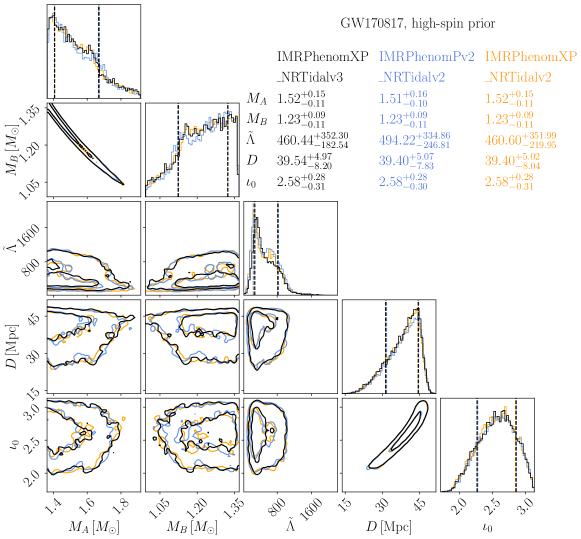
Figure 21: The marginalized 1D and 2D posterior probability distributions for selected parameters of GW170817, with a high-spin prior ($\chi\leq 0.5)$ obtained with IMRPhenomXP_NRTidalv3 (black), IMRPhenomPv2_NRTidalv2 (blue), and IMRPhenomXP_NRTidalv2 (orange). The parameters shown here are the individual star masses $M_{A,B}$, binary tidal deformability $\tilde{\Lambda}$, luminosity distance $D$, and inclination angle $\iota_{0}$. The 68% and 90% confidence intervals are indicated by contours for the 2D posterior plots, while vertical lines in the 1D plots indicate 90% confidence interval. We note a narrow constraint on the tidal deformability for IMRPhenomXP_NRTidalv3 compared to the other models, due to the updated tidal information that was used.

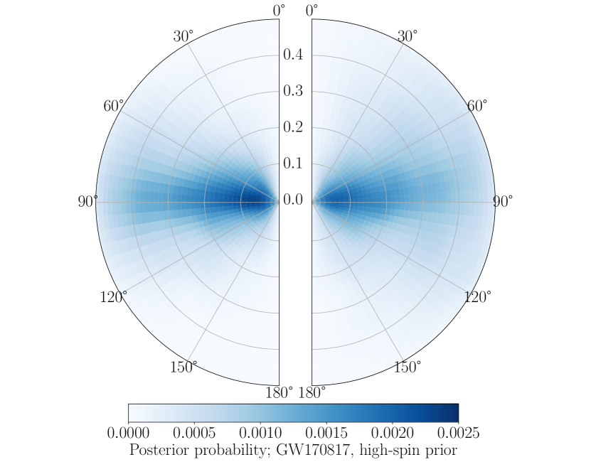
Figure 22: Inferred spin parameters for GW170817 from a high-spin prior ($\chi\leq 0.5$) using IMRPhenomXP_NRTidalv3. Plotted here are the probability densities for the dimensionless spin components $\chi_{1}$ (left hemisphere) and $\chi_{2}$ (right hemisphere) relative to the orbital angular momentum $\mathbf{L}$ and tilt angles (i.e. a tilt angle $0^{\circ}$ means that the spin is aligned with the $\mathbf{L}$). The plot was done at a reference frequency of 20 Hz.

Appendix B Parameter Estimation for high-spin priors

We present here the results for the parameter estimation runs for GW170817 and GW190425, as was done in Sec. VI, but this time, using high-spin priors. For both events, we use a spin prior of up to $\chi\leq 0.50$. We do not employ spins up to 0.89 as done in some LVK studies, given that this spin is well above the breakup spin of neutron stars and is unrealistically large for BNS systems.

GW170817.

The inferred properties of GW170817 with a high-spin prior, together with the marginalized 1D and 2D posterior distributions are shown in Fig. 21. As with the low-spin prior case, the result is consistent with the other waveform models and with previous results [23], and we observe a slightly narrow constraint for IMRPhenomXP_NRTidalv3 in the tidal deformability $\tilde{\Lambda}$. As for the inferred spin parameters, Fig. 22 shows that relatively large components of the spin which are aligned or anti-aligned with the orbital angular momentum $\mathbf{L}$ are heavily disfavored, and constraints are placed on the in-plane spin components.

GW190425.

We show inferred properties of GW190425 with a high-spin prior, together with the marginalized 1D and 2D posterior distributions in Fig. 23. As with the low-spin prior case, the result is consistent with the other waveform models, and we observe a narrower constraint for IMRPhenomXP_NRTidalv3 in the tidal deformability $\tilde{\Lambda}$. Fig. 24 shows similar behavior as in Fig. 22 such that relatively large components of the spin which are aligned or anti-aligned with the orbital angular momentum $\mathbf{L}$ are heavily disfavored, and constraints are placed on the in-plane spin components [5].

Figure 23: The marginalized 1D and 2D posterior probability distributions for selected parameters of GW190425, obtained with IMRPhenomXP_NRTidalv3 (black), IMRPhenomPv2_NRTidalv2 (blue), and IMRPhenomXP_NRTidalv2 (orange), for a high-spin prior ($\chi\leq 0.50$). The parameters shown here are the individual star masses $M_{A,B}$, binary tidal deformability $\tilde{\Lambda}$, luminosity distance $D$, and inclination angle $\iota_{0}$. The 68% and 90% confidence intervals are indicated by contours for the 2D posterior plots, while vertical lines in the 1D plots indicate 90% confidence interval. We note a narrow constraint on the tidal deformability for IMRPhenomXP_NRTidalv3 compared to the other models, due to the updated tidal information that was used.

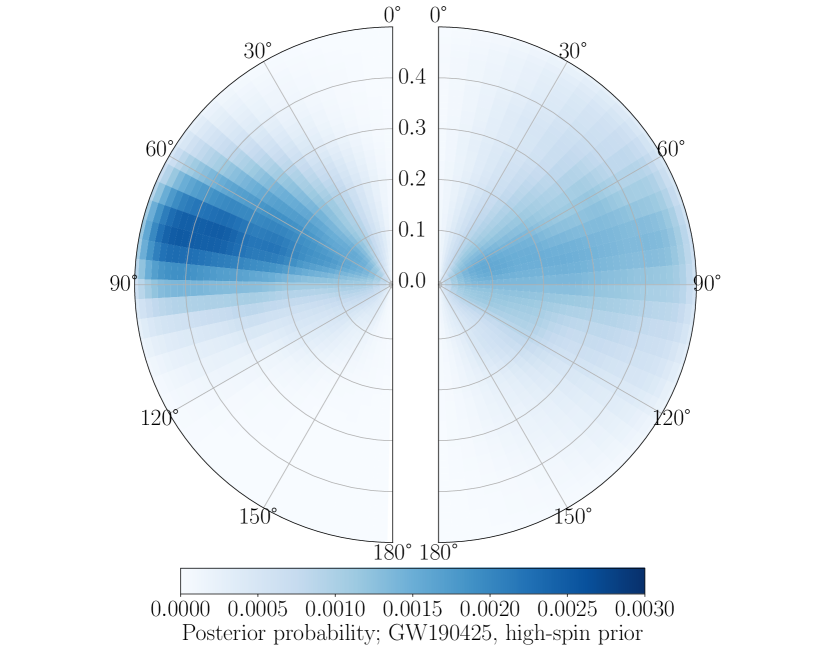
Figure 24: Inferred spin parameters for GW190425 from a high-spin prior ($\chi\leq 0.50$) using IMRPhenomXP_NRTidalv3. Plotted here are the probability densities for the dimensionless spin components $\chi_{1}$ (left hemisphere) and $\chi_{2}$ (right hemisphere) relative to the orbital angular momentum $\mathbf{L}$ and tilt angles (i.e. a tilt angle $0^{\circ}$ means that the spin is aligned with the $\mathbf{L}$). The plot was done at a reference frequency of 20 Hz.

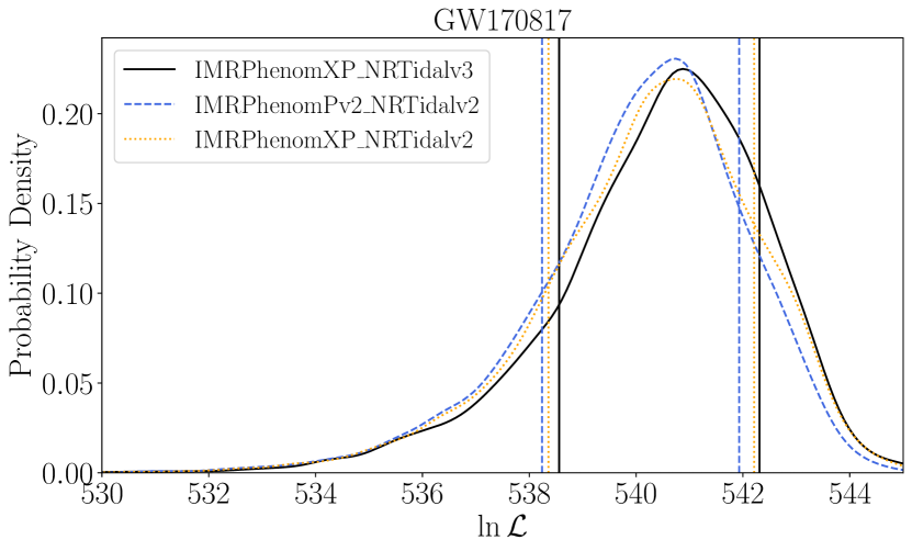
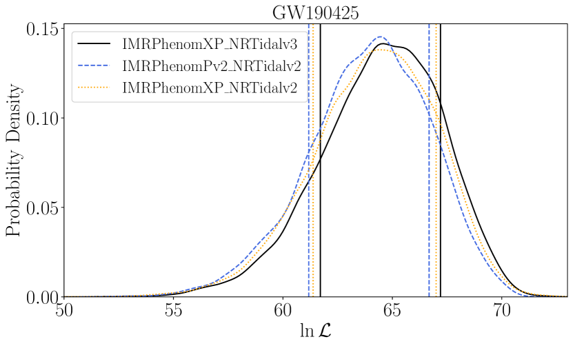
Figure 25: The distribution of the log-likelihood $\ln\mathcal{L}$ for GW170817 (top) and GW190425 (bottom) with high-spin priors ($\chi\leq 0.5$). The vertical lines indicate 90% confidence intervals for the models. We note the shifting of the distribution using IMRPhenomXP_NRTidalv3 towards larger $\ln\mathcal{L}$.

Performance.

Finally, the posterior probability distribution of the log likelihood $\ln\mathcal{L}$ of the three models used with GW170817 and GW190425 and shown in Fig. 25. We note that for both GW events, the $\ln\mathcal{L}$ values for IMRPhenomXP_NRTidalv3 are shifted towards larger values relative to the other two models. For GW170817, we find $\ln\mathcal{B}=525.114\pm 0.091$ with IMRPhenomXP_NRTidalv3, $\ln\mathcal{B}=524.926\pm 0.090$ with IMRPhenomPv2_NRTidalv2, and $\ln\mathcal{B}=525.131\pm 0.090$ with IMRPhenomXP_NRTidalv2. Meanwhile, for GW190425, we obtain $\ln\mathcal{B}=53.831\pm 0.078$ with IMRPhenomXP_NRTidalv3, $\ln\mathcal{B}=53.630\pm 0.077$ with IMRPhenomPv2_NRTidalv2, and $\ln\mathcal{B}=53.632\pm 0.077$ with IMRPhenomXP_NRTidalv2.

References

- Abbott et al. [2016] B. P. Abbott et al. (LIGO Scientific, Virgo), Observation of Gravitational Waves from a Binary Black Hole Merger, Phys. Rev. Lett. 116, 061102 (2016), arXiv:1602.03837 [gr-qc] .
- Abbott et al. [2017a] B. P. Abbott et al. (LIGO Scientific, Virgo), GW170817: Observation of Gravitational Waves from a Binary Neutron Star Inspiral, Phys. Rev. Lett. 119, 161101 (2017a), arXiv:1710.05832 [gr-qc] .
- Abbott et al. [2017b] B. P. Abbott et al. (LIGO Scientific, Virgo, Fermi-GBM, INTEGRAL), Gravitational Waves and Gamma-rays from a Binary Neutron Star Merger: GW170817 and GRB 170817A, Astrophys. J. Lett. 848, L13 (2017b), arXiv:1710.05834 [astro-ph.HE] .
- Abbott et al. [2017c] B. P. Abbott et al. (LIGO Scientific, Virgo, Fermi GBM, INTEGRAL, IceCube, AstroSat Cadmium Zinc Telluride Imager Team, IPN, Insight-Hxmt, ANTARES, Swift, AGILE Team, 1M2H Team, Dark Energy Camera GW-EM, DES, DLT40, GRAWITA, Fermi-LAT, ATCA, ASKAP, Las Cumbres Observatory Group, OzGrav, DWF (Deeper Wider Faster Program), AST3, CAASTRO, VINROUGE, MASTER, J-GEM, GROWTH, JAGWAR, CaltechNRAO, TTU-NRAO, NuSTAR, Pan-STARRS, MAXI Team, TZAC Consortium, KU, Nordic Optical Telescope, ePESSTO, GROND, Texas Tech University, SALT Group, TOROS, BOOTES, MWA, CALET, IKI-GW Follow-up, H.E.S.S., LOFAR, LWA, HAWC, Pierre Auger, ALMA, Euro VLBI Team, Pi of Sky, Chandra Team at McGill University, DFN, ATLAS Telescopes, High Time Resolution Universe Survey, RIMAS, RATIR, SKA South Africa/MeerKAT), Multi-messenger Observations of a Binary Neutron Star Merger, Astrophys. J. Lett. 848, L12 (2017c), arXiv:1710.05833 [astro-ph.HE] .
- Abbott et al. [2020] B. P. Abbott et al. (LIGO Scientific, Virgo), GW190425: Observation of a Compact Binary Coalescence with Total Mass , Astrophys. J. Lett. 892, L3 (2020), arXiv:2001.01761 [astro-ph.HE] .
- Abbott et al. [2018] B. P. Abbott et al. (KAGRA, LIGO Scientific, Virgo, VIRGO), Prospects for observing and localizing gravitational-wave transients with Advanced LIGO, Advanced Virgo and KAGRA, Living Rev. Rel. 21, 3 (2018), arXiv:1304.0670 [gr-qc] .
- Chan et al. [2018] M. L. Chan, C. Messenger, I. S. Heng, and M. Hendry, Binary Neutron Star Mergers and Third Generation Detectors: Localization and Early Warning, Phys. Rev. D 97, 123014 (2018), arXiv:1803.09680 [astro-ph.HE] .
- Lenon et al. [2021] A. K. Lenon, D. A. Brown, and A. H. Nitz, Eccentric binary neutron star search prospects for Cosmic Explorer, Phys. Rev. D 104, 063011 (2021), arXiv:2103.14088 [astro-ph.HE] .
- Branchesi et al. [2023] M. Branchesi et al., Science with the Einstein Telescope: a comparison of different designs, JCAP 07, 068, arXiv:2303.15923 [gr-qc] .
- Dietrich et al. [2020] T. Dietrich, M. W. Coughlin, P. T. H. Pang, M. Bulla, J. Heinzel, L. Issa, I. Tews, and S. Antier, Multimessenger constraints on the neutron-star equation of state and the Hubble constant, Science 370, 1450 (2020), arXiv:2002.11355 [astro-ph.HE] .
- Lattimer [2012] J. M. Lattimer, The nuclear equation of state and neutron star masses, Ann. Rev. Nucl. Part. Sci. 62, 485 (2012), arXiv:1305.3510 [nucl-th] .
- Özel and Freire [2016] F. Özel and P. Freire, Masses, Radii, and the Equation of State of Neutron Stars, Ann. Rev. Astron. Astrophys. 54, 401 (2016), arXiv:1603.02698 [astro-ph.HE] .
- Chin and Walecka [1974] S. A. Chin and J. D. Walecka, An Equation of State for Nuclear and Higher-Density Matter Based on a Relativistic Mean-Field Theory, Phys. Lett. B 52, 24 (1974).
- Serot and Walecka [1997] B. D. Serot and J. D. Walecka, Recent progress in quantum hadrodynamics, Int. J. Mod. Phys. E 6, 515 (1997), arXiv:nucl-th/9701058 .
- Huth et al. [2022] S. Huth et al., Constraining Neutron-Star Matter with Microscopic and Macroscopic Collisions, Nature 606, 276 (2022), arXiv:2107.06229 [nucl-th] .
- Alford et al. [2022] M. G. Alford, L. Brodie, A. Haber, and I. Tews, Relativistic mean-field theories for neutron-star physics based on chiral effective field theory, Phys. Rev. C 106, 055804 (2022), arXiv:2205.10283 [nucl-th] .
- Lattimer [2021] J. M. Lattimer, Neutron Stars and the Nuclear Matter Equation of State, Ann. Rev. Nucl. Part. Sci. 71, 433 (2021).
- Burgio et al. [2021] G. F. Burgio, H. J. Schulze, I. Vidana, and J. B. Wei, Neutron stars and the nuclear equation of state, Prog. Part. Nucl. Phys. 120, 103879 (2021), arXiv:2105.03747 [nucl-th] .
- Zhu et al. [2023] Z. Zhu, A. Li, J. Hu, and H. Shen, Equation of state of nuclear matter and neutron stars: Quark mean-field model versus relativistic mean-field model, (2023), arXiv:2305.16058 [nucl-th] .
- Flanagan and Hinderer [2008] E. E. Flanagan and T. Hinderer, Constraining neutron star tidal Love numbers with gravitational wave detectors, Phys. Rev. D 77, 021502 (2008), arXiv:0709.1915 [astro-ph] .
- Hinderer [2008] T. Hinderer, Tidal Love numbers of neutron stars, Astrophys. J. 677, 1216 (2008), arXiv:0711.2420 [astro-ph] .
- Hinderer et al. [2010] T. Hinderer, B. D. Lackey, R. N. Lang, and J. S. Read, Tidal deformability of neutron stars with realistic equations of state and their gravitational wave signatures in binary inspiral, Phys. Rev. D 81, 123016 (2010), arXiv:0911.3535 [astro-ph.HE] .
- Abbott et al. [2019] B. P. Abbott et al. (LIGO Scientific, Virgo), Properties of the binary neutron star merger GW170817, Phys. Rev. X 9, 011001 (2019), arXiv:1805.11579 [gr-qc] .
- Veitch et al. [2015] J. Veitch et al., Parameter estimation for compact binaries with ground-based gravitational-wave observations using the LALInference software library, Phys. Rev. D 91, 042003 (2015), arXiv:1409.7215 [gr-qc] .
- Thrane and Talbot [2019] E. Thrane and C. Talbot, An introduction to Bayesian inference in gravitational-wave astronomy: parameter estimation, model selection, and hierarchical models, Publ. Astron. Soc. Austral. 36, e010 (2019), [Erratum: Publ.Astron.Soc.Austral. 37, e036 (2020)], arXiv:1809.02293 [astro-ph.IM] .
- Hotokezaka et al. [2015] K. Hotokezaka, K. Kyutoku, H. Okawa, and M. Shibata, Exploring tidal effects of coalescing binary neutron stars in numerical relativity. II. Long-term simulations, Phys. Rev. D 91, 064060 (2015), arXiv:1502.03457 [gr-qc] .
- Hotokezaka et al. [2016] K. Hotokezaka, K. Kyutoku, Y.-i. Sekiguchi, and M. Shibata, Measurability of the tidal deformability by gravitational waves from coalescing binary neutron stars, Phys. Rev. D 93, 064082 (2016), arXiv:1603.01286 [gr-qc] .
- Kawaguchi et al. [2018] K. Kawaguchi, K. Kiuchi, K. Kyutoku, Y. Sekiguchi, M. Shibata, and K. Taniguchi, Frequency-domain gravitational waveform models for inspiraling binary neutron stars, Phys. Rev. D 97, 044044 (2018), arXiv:1802.06518 [gr-qc] .
- Kiuchi et al. [2020] K. Kiuchi, K. Kawaguchi, K. Kyutoku, Y. Sekiguchi, and M. Shibata, Sub-radian-accuracy gravitational waves from coalescing binary neutron stars in numerical relativity. II. Systematic study on the equation of state, binary mass, and mass ratio, Phys. Rev. D 101, 084006 (2020), arXiv:1907.03790 [astro-ph.HE] .
- Foucart et al. [2019] F. Foucart et al., Gravitational waveforms from spectral Einstein code simulations: Neutron star-neutron star and low-mass black hole-neutron star binaries, Phys. Rev. D 99, 044008 (2019), arXiv:1812.06988 [gr-qc] .
- Dietrich et al. [2018a] T. Dietrich, D. Radice, S. Bernuzzi, F. Zappa, A. Perego, B. Brügmann, S. V. Chaurasia, R. Dudi, W. Tichy, and M. Ujevic, CoRe database of binary neutron star merger waveforms, Class. Quant. Grav. 35, 24LT01 (2018a), arXiv:1806.01625 [gr-qc] .
- Ujevic et al. [2022] M. Ujevic, A. Rashti, H. Gieg, W. Tichy, and T. Dietrich, High-accuracy high-mass-ratio simulations for binary neutron stars and their comparison to existing waveform models, Phys. Rev. D 106, 023029 (2022), arXiv:2202.09343 [gr-qc] .
- Gonzalez et al. [2023] A. Gonzalez et al., Second release of the CoRe database of binary neutron star merger waveforms, Class. Quant. Grav. 40, 085011 (2023), arXiv:2210.16366 [gr-qc] .
- Vines et al. [2011] J. Vines, E. E. Flanagan, and T. Hinderer, Post-1-Newtonian tidal effects in the gravitational waveform from binary inspirals, Phys. Rev. D 83, 084051 (2011), arXiv:1101.1673 [gr-qc] .
- Damour et al. [2012] T. Damour, A. Nagar, and L. Villain, Measurability of the tidal polarizability of neutron stars in late-inspiral gravitational-wave signals, Phys. Rev. D 85, 123007 (2012), arXiv:1203.4352 [gr-qc] .
- Henry et al. [2020] Q. Henry, G. Faye, and L. Blanchet, Tidal effects in the gravitational-wave phase evolution of compact binary systems to next-to-next-to-leading post-Newtonian order, Phys. Rev. D 102, 044033 (2020), arXiv:2005.13367 [gr-qc] .
- Narikawa [2023] T. Narikawa, Multipole tidal effects in the gravitational-wave phases of compact binary coalescences, 2307.02033 (2023).
- Buonanno and Damour [1999] A. Buonanno and T. Damour, Effective one-body approach to general relativistic two-body dynamics, Phys. Rev. D 59, 084006 (1999), arXiv:gr-qc/9811091 .
- Buonanno and Damour [2000] A. Buonanno and T. Damour, Transition from inspiral to plunge in binary black hole coalescences, Phys. Rev. D 62, 064015 (2000), arXiv:gr-qc/0001013 .
- Damour and Nagar [2011] T. Damour and A. Nagar, The Effective One Body description of the Two-Body problem, Fundam. Theor. Phys. 162, 211 (2011), arXiv:0906.1769 [gr-qc] .
- Gamba and Bernuzzi [2023] R. Gamba and S. Bernuzzi, Resonant tides in binary neutron star mergers: Analytical-numerical relativity study, Phys. Rev. D 107, 044014 (2023), arXiv:2207.13106 [gr-qc] .
- Gamba et al. [2023] R. Gamba et al., Analytically improved and numerical-relativity informed effective-one-body model for coalescing binary neutron stars, (2023), arXiv:2307.15125 [gr-qc] .
- Hinderer et al. [2016] T. Hinderer et al., Effects of neutron-star dynamic tides on gravitational waveforms within the effective-one-body approach, Phys. Rev. Lett. 116, 181101 (2016), arXiv:1602.00599 [gr-qc] .
- Steinhoff et al. [2016] J. Steinhoff, T. Hinderer, A. Buonanno, and A. Taracchini, Dynamical Tides in General Relativity: Effective Action and Effective-One-Body Hamiltonian, Phys. Rev. D 94, 104028 (2016), arXiv:1608.01907 [gr-qc] .
- Bernuzzi et al. [2015] S. Bernuzzi, A. Nagar, T. Dietrich, and T. Damour, Modeling the Dynamics of Tidally Interacting Binary Neutron Stars up to the Merger, Phys. Rev. Lett. 114, 161103 (2015), arXiv:1412.4553 [gr-qc] .
- Nagar et al. [2018] A. Nagar et al., Time-domain effective-one-body gravitational waveforms for coalescing compact binaries with nonprecessing spins, tides and self-spin effects, Phys. Rev. D 98, 104052 (2018), arXiv:1806.01772 [gr-qc] .
- Akcay et al. [2019] S. Akcay, S. Bernuzzi, F. Messina, A. Nagar, N. Ortiz, and P. Rettegno, Effective-one-body multipolar waveform for tidally interacting binary neutron stars up to merger, Phys. Rev. D 99, 044051 (2019), arXiv:1812.02744 [gr-qc] .
- Lackey et al. [2017] B. D. Lackey, S. Bernuzzi, C. R. Galley, J. Meidam, and C. Van Den Broeck, Effective-one-body waveforms for binary neutron stars using surrogate models, Phys. Rev. D 95, 104036 (2017), arXiv:1610.04742 [gr-qc] .
- Lackey et al. [2019] B. D. Lackey, M. Pürrer, A. Taracchini, and S. Marsat, Surrogate model for an aligned-spin effective one body waveform model of binary neutron star inspirals using Gaussian process regression, Phys. Rev. D 100, 024002 (2019), arXiv:1812.08643 [gr-qc] .
- Nagar and Rettegno [2019] A. Nagar and P. Rettegno, Efficient effective one body time-domain gravitational waveforms, Phys. Rev. D 99, 021501 (2019), arXiv:1805.03891 [gr-qc] .
- Mihaylov et al. [2021] D. P. Mihaylov, S. Ossokine, A. Buonanno, and A. Ghosh, Fast post-adiabatic waveforms in the time domain: Applications to compact binary coalescences in LIGO and Virgo, Phys. Rev. D 104, 124087 (2021), arXiv:2105.06983 [gr-qc] .
- Tissino et al. [2023] J. Tissino, G. Carullo, M. Breschi, R. Gamba, S. Schmidt, and S. Bernuzzi, Combining effective-one-body accuracy and reduced-order-quadrature speed for binary neutron star merger parameter estimation with machine learning, Phys. Rev. D 107, 084037 (2023), arXiv:2210.15684 [gr-qc] .
- Gamba et al. [2021] R. Gamba, S. Bernuzzi, and A. Nagar, Fast, faithful, frequency-domain effective-one-body waveforms for compact binary coalescences, Phys. Rev. D 104, 084058 (2021), arXiv:2012.00027 [gr-qc] .
- Ajith et al. [2011] P. Ajith et al., Inspiral-merger-ringdown waveforms for black-hole binaries with non-precessing spins, Phys. Rev. Lett. 106, 241101 (2011), arXiv:0909.2867 [gr-qc] .
- Santamaria et al. [2010] L. Santamaria et al., Matching post-Newtonian and numerical relativity waveforms: systematic errors and a new phenomenological model for non-precessing black hole binaries, Phys. Rev. D 82, 064016 (2010), arXiv:1005.3306 [gr-qc] .
- Dietrich et al. [2017] T. Dietrich, S. Bernuzzi, and W. Tichy, Closed-form tidal approximants for binary neutron star gravitational waveforms constructed from high-resolution numerical relativity simulations, Phys. Rev. D 96, 121501 (2017), arXiv:1706.02969 [gr-qc] .
- Dietrich et al. [2019a] T. Dietrich, A. Samajdar, S. Khan, N. K. Johnson-McDaniel, R. Dudi, and W. Tichy, Improving the NRTidal model for binary neutron star systems, Phys. Rev. D 100, 044003 (2019a), arXiv:1905.06011 [gr-qc] .
- LIGO Scientific Collaboration [2018] LIGO Scientific Collaboration, LIGO Algorithm Library - LALSuite, free software (GPL) (2018).
- Shibata [1994] M. Shibata, Effects of Tidal Resonances in Coalescing Compact Binary Systems, Progress of Theoretical Physics 91, 871 (1994).
- Schmidt and Hinderer [2019] P. Schmidt and T. Hinderer, Frequency domain model of -mode dynamic tides in gravitational waveforms from compact binary inspirals, Phys. Rev. D 100, 021501 (2019), arXiv:1905.00818 [gr-qc] .
- Andersson and Pnigouras [2021] N. Andersson and P. Pnigouras, The phenomenology of dynamical neutron star tides, Mon. Not. Roy. Astron. Soc. 503, 533 (2021), arXiv:1905.00012 [gr-qc] .
- Gupta et al. [2021] P. K. Gupta, J. Steinhoff, and T. Hinderer, Relativistic effective action of dynamical gravitomagnetic tides for slowly rotating neutron stars, Phys. Rev. Res. 3, 013147 (2021), arXiv:2011.03508 [gr-qc] .
- Steinhoff et al. [2021] J. Steinhoff, T. Hinderer, T. Dietrich, and F. Foucart, Spin effects on neutron star fundamental-mode dynamical tides: Phenomenology and comparison to numerical simulations, Phys. Rev. Res. 3, 033129 (2021), arXiv:2103.06100 [gr-qc] .
- Pratten et al. [2022] G. Pratten, P. Schmidt, and N. Williams, Impact of Dynamical Tides on the Reconstruction of the Neutron Star Equation of State, Phys. Rev. Lett. 129, 081102 (2022), arXiv:2109.07566 [astro-ph.HE] .
- Kuan and Kokkotas [2022] H.-J. Kuan and K. D. Kokkotas, f-mode imprints on gravitational waves from coalescing binaries involving aligned spinning neutron stars, Phys. Rev. D 106, 064052 (2022), arXiv:2205.01705 [gr-qc] .
- Pnigouras et al. [2022] P. Pnigouras, F. Gittins, A. Nanda, N. Andersson, and D. I. Jones, Rotating Love: The dynamical tides of spinning Newtonian stars, (2022), arXiv:2205.07577 [gr-qc] .
- Mandal et al. [2023a] M. K. Mandal, P. Mastrolia, H. O. Silva, R. Patil, and J. Steinhoff, Gravitoelectric dynamical tides at second post-Newtonian order, (2023a), arXiv:2304.02030 [hep-th] .
- Mandal et al. [2023b] M. K. Mandal, P. Mastrolia, H. O. Silva, R. Patil, and J. Steinhoff, Renormalizing Love: tidal effects at the third post-Newtonian order, (2023b), arXiv:2308.01865 [hep-th] .
- Kiuchi et al. [2017] K. Kiuchi, K. Kawaguchi, K. Kyutoku, Y. Sekiguchi, M. Shibata, and K. Taniguchi, Sub-radian-accuracy gravitational waveforms of coalescing binary neutron stars in numerical relativity, Phys. Rev. D 96, 084060 (2017), arXiv:1708.08926 [astro-ph.HE] .
- Dietrich et al. [2019b] T. Dietrich et al., Matter imprints in waveform models for neutron star binaries: Tidal and self-spin effects, Phys. Rev. D 99, 024029 (2019b), arXiv:1804.02235 [gr-qc] .
- Bernuzzi and Dietrich [2016] S. Bernuzzi and T. Dietrich, Gravitational waveforms from binary neutron star mergers with high-order weighted-essentially-nonoscillatory schemes in numerical relativity, Phys. Rev. D 94, 064062 (2016), arXiv:1604.07999 [gr-qc] .
- Dietrich et al. [2018b] T. Dietrich, S. Bernuzzi, B. Bruegmann, and W. Tichy, High-resolution numerical relativity simulations of spinning binary neutron star mergers, in 26th Euromicro International Conference on Parallel, Distributed and Network-based Processing (2018) pp. 682–689, arXiv:1803.07965 [gr-qc] .
- Lackey et al. [2014] B. D. Lackey, K. Kyutoku, M. Shibata, P. R. Brady, and J. L. Friedman, Extracting equation of state parameters from black hole-neutron star mergers: aligned-spin black holes and a preliminary waveform model, Phys. Rev. D 89, 043009 (2014), arXiv:1303.6298 [gr-qc] .
- Savitzky and Golay [1964] A. Savitzky and M. J. E. Golay, Smoothing and differentiation of data by simplified least squares procedures., Analytical Chemistry 36, 1627 (1964), https://doi.org/10.1021/ac60214a047 .
- Sotani and Kumar [2021] H. Sotani and B. Kumar, Universal relations between the quasinormal modes of neutron star and tidal deformability, Phys. Rev. D 104, 123002 (2021), arXiv:2109.08145 [gr-qc] .
- O’Dell and Hamilton [2023] A. O’Dell and M. C. B. Hamilton, Rising Tides: Analytic Modeling of Tidal Effects in Binary Neutron Star Mergers, (2023), arXiv:2307.16022 [astro-ph.HE] .
- Droz et al. [1999] S. Droz, D. J. Knapp, E. Poisson, and B. J. Owen, Gravitational waves from inspiraling compact binaries: Validity of the stationary phase approximation to the Fourier transform, Phys. Rev. D 59, 124016 (1999), arXiv:gr-qc/9901076 .
- Pappas and Apostolatos [2014] G. Pappas and T. A. Apostolatos, Effectively universal behavior of rotating neutron stars in general relativity makes them even simpler than their Newtonian counterparts, Phys. Rev. Lett. 112, 121101 (2014), arXiv:1311.5508 [gr-qc] .
- Yagi et al. [2014] K. Yagi, K. Kyutoku, G. Pappas, N. Yunes, and T. A. Apostolatos, Effective No-Hair Relations for Neutron Stars and Quark Stars: Relativistic Results, Phys. Rev. D 89, 124013 (2014), arXiv:1403.6243 [gr-qc] .
- Nagar et al. [2019] A. Nagar, F. Messina, P. Rettegno, D. Bini, T. Damour, A. Geralico, S. Akcay, and S. Bernuzzi, Nonlinear-in-spin effects in effective-one-body waveform models of spin-aligned, inspiralling, neutron star binaries, Phys. Rev. D 99, 044007 (2019), arXiv:1812.07923 [gr-qc] .
- Yagi and Yunes [2017] K. Yagi and N. Yunes, Approximate Universal Relations for Neutron Stars and Quark Stars, Phys. Rept. 681, 1 (2017), arXiv:1608.02582 [gr-qc] .
- [82] M. Colleoni, F. Ramis, N. Johnson-McDaniel, G. Pratten, C. Garcia-Quiros, T. Dietrich, et al., article in preparation .
- Khan et al. [2016] S. Khan, S. Husa, M. Hannam, F. Ohme, M. Pürrer, X. Jiménez Forteza, and A. Bohé, Frequency-domain gravitational waves from nonprecessing black-hole binaries. II. A phenomenological model for the advanced detector era, Phys. Rev. D 93, 044007 (2016), arXiv:1508.07253 [gr-qc] .
- Pratten et al. [2020] G. Pratten, S. Husa, C. Garcia-Quiros, M. Colleoni, A. Ramos-Buades, H. Estelles, and R. Jaume, Setting the cornerstone for a family of models for gravitational waves from compact binaries: The dominant harmonic for nonprecessing quasicircular black holes, Phys. Rev. D 102, 064001 (2020), arXiv:2001.11412 [gr-qc] .
- Pompili et al. [2023] L. Pompili et al., Laying the foundation of the effective-one-body waveform models SEOBNRv5: improved accuracy and efficiency for spinning non-precessing binary black holes, 2303.18039 (2023).
- Pratten et al. [2021] G. Pratten et al., Computationally efficient models for the dominant and subdominant harmonic modes of precessing binary black holes, Phys. Rev. D 103, 104056 (2021), arXiv:2004.06503 [gr-qc] .
- Damour and Nagar [2014] T. Damour and A. Nagar, New effective-one-body description of coalescing nonprecessing spinning black-hole binaries, Phys. Rev. D 90, 044018 (2014), arXiv:1406.6913 [gr-qc] .
- Nagar et al. [2016] A. Nagar, T. Damour, C. Reisswig, and D. Pollney, Energetics and phasing of nonprecessing spinning coalescing black hole binaries, Phys. Rev. D 93, 044046 (2016), arXiv:1506.08457 [gr-qc] .
- Nagar et al. [2020a] A. Nagar, G. Pratten, G. Riemenschneider, and R. Gamba, Multipolar effective one body model for nonspinning black hole binaries, Phys. Rev. D 101, 024041 (2020a), arXiv:1904.09550 [gr-qc] .
- Nagar et al. [2020b] A. Nagar, G. Riemenschneider, G. Pratten, P. Rettegno, and F. Messina, Multipolar effective one body waveform model for spin-aligned black hole binaries, Phys. Rev. D 102, 024077 (2020b), arXiv:2001.09082 [gr-qc] .
- Riemenschneider et al. [2021] G. Riemenschneider, P. Rettegno, M. Breschi, A. Albertini, R. Gamba, S. Bernuzzi, and A. Nagar, Assessment of consistent next-to-quasicircular corrections and postadiabatic approximation in effective-one-body multipolar waveforms for binary black hole coalescences, Phys. Rev. D 104, 104045 (2021), arXiv:2104.07533 [gr-qc] .
- Husa et al. [2016] S. Husa, S. Khan, M. Hannam, M. Pürrer, F. Ohme, X. Jiménez Forteza, and A. Bohé, Frequency-domain gravitational waves from nonprecessing black-hole binaries. I. New numerical waveforms and anatomy of the signal, Phys. Rev. D 93, 044006 (2016), arXiv:1508.07250 [gr-qc] .
- Schmidt et al. [2015] P. Schmidt, F. Ohme, and M. Hannam, Towards models of gravitational waveforms from generic binaries II: Modelling precession effects with a single effective precession parameter, Phys. Rev. D 91, 024043 (2015), arXiv:1408.1810 [gr-qc] .
- Ashton et al. [2019] G. Ashton et al., BILBY: A user-friendly Bayesian inference library for gravitational-wave astronomy, Astrophys. J. Suppl. 241, 27 (2019), arXiv:1811.02042 [astro-ph.IM] .
- Smith et al. [2020] R. J. E. Smith, G. Ashton, A. Vajpeyi, and C. Talbot, Massively parallel Bayesian inference for transient gravitational-wave astronomy, Mon. Not. Roy. Astron. Soc. 498, 4492 (2020), arXiv:1909.11873 [gr-qc] .
- Speagle [2020] J. S. Speagle, dynesty: a dynamic nested sampling package for estimating Bayesian posteriors and evidences, Mon. Not. Roy. Astron. Soc. 493, 3132 (2020), arXiv:1904.02180 [astro-ph.IM] .
- Romero-Shaw et al. [2020] I. M. Romero-Shaw et al., Bayesian inference for compact binary coalescences with bilby: validation and application to the first LIGO–Virgo gravitational-wave transient catalogue, Mon. Not. Roy. Astron. Soc. 499, 3295 (2020), arXiv:2006.00714 [astro-ph.IM] .
- Ashton and Dietrich [2022] G. Ashton and T. Dietrich, The use of hypermodels to understand binary neutron star collisions, Nature Astron. 6, 961 (2022), arXiv:2111.09214 [gr-qc] .
- Thompson et al. [2020] J. E. Thompson, E. Fauchon-Jones, S. Khan, E. Nitoglia, F. Pannarale, T. Dietrich, and M. Hannam, Modeling the gravitational wave signature of neutron star black hole coalescences, Phys. Rev. D 101, 124059 (2020), arXiv:2002.08383 [gr-qc] .
- Matas et al. [2020] A. Matas et al., Aligned-spin neutron-star–black-hole waveform model based on the effective-one-body approach and numerical-relativity simulations, Phys. Rev. D 102, 043023 (2020), arXiv:2004.10001 [gr-qc] .
- Markin et al. [2023] I. Markin, A. Neuweiler, A. Abac, S. V. Chaurasia, M. Ujevic, M. Bulla, and T. Dietrich, General-Relativistic Hydrodynamics Simulation of a Neutron Star - Sub-Solar-Mass Black Hole Merger, (2023), arXiv:2304.11642 [gr-qc] .
- Abbott et al. [2021] R. Abbott et al. (LIGO Scientific, KAGRA, VIRGO), Observation of Gravitational Waves from Two Neutron Star–Black Hole Coalescences, Astrophys. J. Lett. 915, L5 (2021), arXiv:2106.15163 [astro-ph.HE] .
- Bohé et al. [2017] A. Bohé et al., Improved effective-one-body model of spinning, nonprecessing binary black holes for the era of gravitational-wave astrophysics with advanced detectors, Phys. Rev. D 95, 044028 (2017), arXiv:1611.03703 [gr-qc] .
- Pürrer [2014] M. Pürrer, Frequency domain reduced order models for gravitational waves from aligned-spin compact binaries, Class. Quant. Grav. 31, 195010 (2014), arXiv:1402.4146 [gr-qc] .
- Pürrer [2016] M. Pürrer, Frequency domain reduced order model of aligned-spin effective-one-body waveforms with generic mass-ratios and spins, Phys. Rev. D 93, 064041 (2016), arXiv:1512.02248 [gr-qc] .