Discrete Nonparametric Causal Discovery Under Latent Class Confounding

Abstract

Directed acyclic graphs are used to model the causal structure of a system. “Causal discovery” describes the problem of learning this structure from data. When data is an aggregate from multiple sources (populations or environments), global confounding obscures conditional independence properties that drive many causal discovery algorithms. This setting is sometimes known as a mixture model or a latent class. While some modern methods for causal discovery are able to work around unobserved confounding in specific cases, the only known ways to deal with a global confounder involve parametric assumptions. that are unsuitable for discrete distributions.Focusing on discrete and non-parametric observed variables, we demonstrate that causal discovery can still be identifiable under bounded latent classes. The feasibility of this problem is governed by a trade-off between the cardinality of the global confounder, the cardinalities of the observed variables, and the sparsity of the causal structure.

1 Introduction

The recent success of of ML and AI has largely been attributed to the emergence of large and comprehensive datasets [25]. Data on natural language and images exist in abundance thanks to the internet. However, the scale of scientific data tends to pale in comparison due to the amount of time needed to generate usable data. Recent efforts, particularly in the biological sciences, have aimed to improve the scope, reach, and scale of existing datasets by combining data from many sources. Examples include The Cancer Genome Atlas (TCGA) [34], the 1000 Genome Project [7], and the upcoming Regeneron Genetics Center Million Exome (RGC-ME) [32].

Whenever data spans multiple populations, environments, or laboratories, the relationships within are subject to “latent class confounding” or “global confounding” [15]. In biology, these effects are often referred to as “batch effects.” In these settings, it is impossible to determine whether signals are true causal relationships or spurious indicators of population (or lab source, etc.) membership.

One approach to the removal of latent class confounding has been to identify the joint probability distribution between the latent class and the observed variable. Such a task is equivalent to that of learning a mixture model by uncovering the “mixture weights” and “source distributions.”

Mixture Models

Most work on learning mixture models deals with parametric distributions; mixtures of Gaussians being the prevalent example. The computational complexity of learning such mixtures has been the subject of numerous works published in the past 25 years, starting with the ground-breaking work of [9].

To learn a mixture model, assumptions about the source-level distribution must be made. A popular choice involves parametric assumptions, such as Gaussian noise. A separate line of work has involved the study of mixtures on discrete distributions, for which no parametric assumptions can be made. Almost all of the research in this setting assumes that the observed variables are mutually independent within the source distributions [8, 13, 5, 12, 23, 6, 14, 16]; see also the earlier seminal work of [17].

A separate line of work pioneered by [11] has viewed this problem as a decomposition into rank-1 tensors. This approach often only seeks identifiability within a measure-1 subset of mixture models, yielding slightly different necessary conditions.

Structural Causal Models

Many modern approaches to studying causal systems use structural causal models (SCMs) to graphically model causal relationships in a directed acyclic graph (DAG) [22]. In an SCM, $A\rightarrow B$ indicates “$A$ causes $B$.” These graphical models provide a systematic way of determining adjustments to indentify the effects of interventions [22].

Graphical Assumptions for Mixtures

Assuming independence within source distributions amounts to a graphical assumption, i.e. that the causal model within each source is an empty graph. Early work by [3] and [15] has sought to broaden this class of independence assumptions for mixture identifiability, exploring Markov random fields and Bayesian networks respectively. While [3] provides an algorithm for learning the Markov random field, [15] instead assumes a known Bayesian DAG structure in order to recover the mixture. To date there is no result showing if and when the within-source DAG structure can be identified from the observed data of a mixture model.

Contributions

The goal of this paper will be provide the first identifiability result on learning causal structures within the discrete mixture setting. We will do this by building on the notion of “rank tests,” introduced by [3]. We also seek to extend the relevance of these tests to binary observable variables, which are usually limited by the maximum rank of a $2\times 2$ matrix. To solve this problem, we develop the notion of “coarsening” to understand the relationship between graph sparsity, visible variable cardinality, and latent class cardinality, when determining identifiability.

Related Work

The question of recovering a causal structure falls within the general umbrella of “causal discovery” [31]. The simplest algorithms for causal discovery make use of a many-to-one mapping of causal SCMs to their implied conditional independence properties, the most famous of which is the PC algorithm [26]. By testing for conditional independence, these approaches isolate an equivalence class, known as a CP-DAG, which gives both a correct skeleton of the causal structure and a partial orientation of its edges.

Latent confounding can link non-causally adjacent variables, obscuring their true relationships and structures and rendering independence-based algorithms inadequate. While a large body of work has studied causal discovery under latent confounding with limited scope [30, 29, 27], the problem of global latent confounding has only been tackled using parametric assumptions such as linear structural equations with non-Gaussian additive noise [4] and non-linear structural equations with Gaussian noise [2]. Other work has investigated a different setting in which different DAG structures are mixed [24]. This work relies on the preservation of some local conditional independence properties to learn a “union graph.”

2 THE PROBLEM

Figure 1: An example. The goal is to learn the graph structure $\mathcal{G}$ without observing $U$.

$\mathcal{G}^{\prime}=(\bm{V}\cup\{U\},\bm{E}^{\prime})$ will refer to the entire graph structure, including the global confounder $U$ which points to all of the “visible” or “observed” variables $\bm{V}$. We will refer to $\mathcal{G}=(\bm{V},\bm{E})$ as the “observed subgraph.” Throughout the paper, we will use $\Delta:=\max_{V\in\bm{V}}\deg^{\mathcal{G}}(V)$ as the maximum degree in the observed subgraph.

The goal will be to uncover the graph structure $\mathcal{G}$ up to Markov equivalence classes (i.e. a CP-DAG) using statistics gained from the “observed probability distribution,” i.e. $\Pr(\bm{V})$ marginalized over $U$. To accomplish this, we will assume (1) that the distribution is faithful with respect to $\mathcal{G}^{\prime}$, and (2) that $U$ is discrete with a bounded number of latent classes $\mathopen{|}\mathcal{U}\mathclose{|}\leq k$. To illustrate how low-dimensional visible variables can still recover high dimensional confounders we will restrict our focus to binary $\bm{V}$. We stress that larger cardinalities in $\bm{V}$ make this problem significantly easier (as will be later explained) – much of our contribution centers around creating larger cardinality variables through graph coarsenings.

Theorem 1.

Consider $\mathcal{G}=(\bm{V},\bm{E})$ with mixture source $U\in\{1,\ldots,k\}$ and degree bound $\Delta$. The CP-DAG associated with $\mathcal{G}$ is generically identifiable with $\Omega(\log(k)\Delta^{3})$ vertices. Using an oracle that can solve $k$-MixProd in time $\tau$ and an oracle that can solve for non-negative rank in time $\rho$ we give an algorithm that runs in time $\mathopen{|}\bm{V}\mathclose{|}^{\mathcal{O}(\Delta^{2}\log(k))}\rho+\mathcal{O}(k\mathopen{|}\bm{E}\mathclose{|}2^{\Delta^{2}})\tau$.

The non-negative rank of a $k+1\times k+1$ matrix (as used for our algorithm) can be solved in time $k^{\mathcal{O}(k^{2})}$ [20]. In the absence of non-negative rank tests, [3] demonstrated that regular rank tests generally work well in place of non-negative rank tests in practice. We will provide additional experimentation to support this claim, as well as an empirical investigation into how these rank tests fail.

Our solution also requires solving $k$-MixProd on 3 variables of cardinality $\mathcal{O}(k)$, which corresponds to decomposing a $\mathcal{O}(k)\times\mathcal{O}(k)\times\mathcal{O}(k)$ tensor into rank $1$ components. When the rank of such a tensor is known to be linear in $k$, this decomposition can be solved in $O(k^{6.05})$ [10], though [14] showed that the problem generally suffers from instability, with sample complexity exponential in $k$. This step may be considered optional, as it is used to refine a small number of “false-positive” adjacencies confined to a provably small subset of the DAG. This paper will center around the development of this algorithm.

3 PRELIMINARIES

3.1 Notation

We will use the capital Latin alphabet to denote random variables, which are vertices on our DAG. When referring to sets of these variables, we will use bolded font, e.g. $\bm{X}=\{X_{1},X_{2},\ldots\}$. To refer to components of a graph, we will use the following operators: $\operatorname{\mathbf{PA}}(V),\operatorname{\mathbf{CH}}(V)$ will refer to the parents and children of $V$. $\operatorname{\mathbf{AN}}(V),\operatorname{\mathbf{DE}}(V)$ will refer to the ancestors and descendants of $V$. $\operatorname{\mathbf{AN}}(V)\cup\{V\}$ and $\operatorname{\mathbf{DE}}(V)\cup\{V\}$ are denoted using $\operatorname{\mathbf{AN^{+}}}(V),\operatorname{\mathbf{DE^{+}}}(V)$ respectively. $\operatorname{\mathbf{MB}}(V)=\operatorname{\mathbf{PA}}(V)\cup\operatorname{\mathbf{CH}}(V)\cup\operatorname{\mathbf{PA}}(\operatorname{\mathbf{CH}}(V))$ will refer to the Markov boundary (i.e. the unique minimal Markov blanket) of $V$ [22]. $\operatorname{\mathbf{NB}}_{\ell}(V)$ refers to the distance $\ell$ neighborhood of $V$.

As these operators act on graphs, they can specify the graph structure being used in the superscript, e.g. $\operatorname{\mathbf{PA}}^{\mathcal{G}}(V)$. We will also occasionally write tuples to indicate the intersection of the sets for two vetices, e.g. $\operatorname{\mathbf{CH}}(V,W)=\operatorname{\mathbf{CH}}(V)\cap\operatorname{\mathbf{CH}}(W)$. Finally, these operators can also act on sets to indicate the union of the operation, e.g.

$$\operatorname{\mathbf{PA}}(\bm{X})=\bigcup_{X\in\bm{X}}\operatorname{\mathbf{PA}}(X)\setminus\bm{X}.$$ (1)

We make use of lowercase letters to denote assignments, for example $x$ will denote the assignment $X=x$. This can also be applied to operators, e.g. $\operatorname{\mathbf{mb}}(V)$ denotes an assignment to $\operatorname{\mathbf{MB}}(V)$. Assignments for these operators can also be obtained from a larger set of assignments using a subscript, e.g. $\operatorname{\mathbf{mb}}_{\bm{c}}(V)$ obtains assignments for $\operatorname{\mathbf{MB}}(V)\subseteq\bm{C}$ from the assignments of $\bm{c}$ to $\bm{C}$. ${\operatorname{rk}_{+}}(\bm{\mathcal{M}})$ will denote the nonnegative rank of matrix $\bm{\mathcal{M}}$.

3.2 Identifying Mixture of Discrete Products

The main tool used in [15] is a solution to identifying discrete $k$-mixtures of product distributions ($k$-MixProd) - i.e. $\bm{X}=X_{1},\ldots,X_{n}$ and latent global confounder or “source” $U$ such that $X_{i}\perp\!\!\!\perp X_{j}\mid U$ for all $i,j$. The key complexity parameter for identifiability is $k$, the cardinality of the support of $U$.

At its core, $k$-MixProd shows how coincidences of multiple independent events reveal information about their confoundedness. Of course, it is possible for $U$ with sufficiently large $k$ to completely control the distribution on $\bm{X}$. For example, for binary $X_{i}\in\{0,1\}$, a cardinality of $k=2^{n}$ would be sufficient to assign each binary sequence in $\bm{X}$ to a latent class in $U$. Such a powerful $U$ could generate any desired probability distribution on $\bm{X}$ by simply controlling the probability distribution on $U$. Limiting $k$, however, limits the space of marginal probability distributions on $\bm{X}$, eventually giving rise to identifiability.

Under a cardinality bound $k$ on the support of $U$, [11] showed that $n\geq\Omega(\log(k))$ is sufficient for the generic identification of $k$-MixProd. In other words, other than a Lebesgue measue $0$ set of exceptions, most instances of $k$-MixProd have a one-to-one correspondence with their observed statistics (the probability distribution on $\bm{X}$ marginalized over $U$) and generating model (up to a set of $k!$ models with permuted labels of $U$).

For guaranteed identifiability, [33] demonstrated that a linear lower bound ($n\geq 2k-1$), in conjunction with a separation condition in the distributions of $X_{i}\mid U$, is sufficient to guarantee identifiability. The best known algorithm for identification is given in [16], which nearly matches the known lower bounds for sample complexity. This paper will use the result from [11], but our methods easily extend to stronger identifiability conditions with modifications in the sparsity requirements.

3.3 D-separation

We will rely on the concepts of d-separation, active paths, and separating sets. Active paths are defined relative to sets of variables to be conditioned on (“conditioning sets”).

A key concept in active paths is that of a collider, $C$, which takes the form $V_{1}\rightarrow C\leftarrow V_{2}$ along an undirected path. Undirected paths through unconditioned variables with no colliders are considered active because they can “carry dependence” from one end of the path to the other. If a non-collider along one of these non-collider paths is conditioned on, then the path is inactive.

Collider steps of paths behave in the opposite fashion: paths with an unconditioned collider are inactive, whereas conditioning on a collider or any descendant of that collider “opens" the active path.

When two variables have an active path between them, we say that they are d-connected. If there are no active paths between the variables, we say they are d-separated. A separating set between two variables is a set of variables which, when conditioned on, break all active paths between those variables. While only loosely described here, a full precise definition of d-separation can be found in [21] and [22] (for a more extensive study).

[21] uses structural causal models to justify the local Markov condition, which means that d-separation always implies independence and allows DAG structures to be factorized. It is possible that two d-connected variables by chance exhibit some unexpected statistical independence. This complication is often assumed away using “faithfulness” [28], which ensures that d-connectedness implies statistical dependence. Together, the local Markov condition and faithfulness give a correspondence statistical dependence and the graphical conditions of the causal DAG which can be leveraged for causal structure learning.

The following fact will be useful when building separating sets.

Lemma 1 ([22]).

If vertices $V_{i},V_{j}$ are nonadjacent in $\mathcal{G}$, either $\operatorname{\mathbf{PA}}^{\mathcal{G}}(V_{i})$ or $\operatorname{\mathbf{PA}}^{\mathcal{G}}(V_{j})$ are a valid separating set for $V_{i},V_{j}$.

We will often want to bound the cardinality of separating sets relative to the degree bound of the graph ($\Delta$). When dealing with a separating set between two vertices $V_{i},V_{j}$, Lemma 1 implies a simple upper bound of $\Delta$. Separating sets for sets (or coarsenings) of vertices are significantly more complicated because conditioning may d-separate some pairs of vertices while d-connecting others.

To unify the treatment of separating sets, we will make use of moral graphs, which can be thought of as undirected equivalents of DAGs [19]. We will denote the moral graph of $\mathcal{G}$ as $\mathcal{G}^{(m)}$. To transform $\mathcal{G}$ into $\mathcal{G}^{(m)}$, we add edges between all immoralities, i.e. nonadjacent vertices with a common child, sometimes called an unsheilded collider. After this, we change all directed edges to undirected edges.

A very useful fact from [19] (also Eq. 1 in [1]) is that all separating sets $\bm{C}\subseteq\bm{V}$ for $\bm{S},\bm{S}^{\prime}\subseteq\bm{V}$ in $\mathcal{G}$ are also separating sets in $(\mathcal{G}[\operatorname{\mathbf{AN^{+}}}(\bm{S}\cup\bm{S}^{\prime}\cup\bm{C})])^{(m)}$. This transforms complicated active path analysis into simple connectedness arguments on undirected moral graphs (of special subgraphs of $\mathcal{G}$). A convenient consequence of this transformation, which we will use throughout the paper, is Lemma 2.

Lemma 2.

If $\mathcal{G}=(\bm{V},\bm{E})$ has degree bound $\Delta$, then the size of a separating set between $\bm{S},\bm{S}^{\prime}\subseteq\bm{V}$ is no larger than $\min(\mathopen{|}\bm{S}\mathclose{|},\mathopen{|}\bm{S}^{\prime}\mathclose{|})\Delta^{2}$.

Lemma 2 is a consequence of the maximum increase in the degree of the moral graph. The full proof is given in Appendix A.

Another helpful result from moral graphs is Lemma 3, which will help us when we prove the existence of separating sets.

Lemma 3 (Corollary of Theorem 1 in [1]).

For DAG $\mathcal{G}=(\bm{V},\bm{E})$, and $\bm{S},\bm{S}^{\prime}\subseteq\bm{V}$, separating sets $\bm{S},\bm{S}$ in $(\mathcal{G}[\operatorname{\mathbf{AN^{+}}}(\bm{S_{i}}\cup\bm{S_{j}})])^{(m)}$ are also separating sets in $\mathcal{G}$.

3.4 Outline of Algorithm

The PC-algorithm works in two phases. The first phase begins with a complete graph (i.e. all possible edges) and uses conditional independence tests to find non-adjacencies and “separating sets” that d-separate them. When a non-adjacency is found, the corresponding edge is removed from the graph and its separating set is stored. The second phase uses the separating sets from the first phase to orient immoralities (as well as further propagation of edge orientation via Meek rules).

The use of independence tests in the PC algorithm (and its variations) relies on a correspondence between independence (a property of probability distributions) and d-separation (a property of DAGs). For example, $V_{i}\perp\!\!\!\perp V_{j}\mid\bm{C}\Leftrightarrow V_{i}\perp\!\!\!\perp^{\mathcal{G}}_{d}V_{j}\mid\bm{C}$ generally holds in unconfounded scenarios (under the “faithfulness” assumption with respect to $\mathcal{G}$).

This property fails in our setting because $U$ confounds all pairs of variables in $\bm{V}$. Hence $V_{i}\not\perp\!\!\!\perp V_{j}\mid\bm{C}$ for any $\bm{C}\subseteq\bm{V}$ because $U$ is in every separating set. To discover non-adjacency between variables in $\bm{V}$, we will need to develop a test that determines when $V_{i}\perp\!\!\!\perp_{d}V_{j}\mid\bm{C}\cup\{U\}$ without access to probability distributions that are conditional on $U$.

We develop this test by digging further into the properties of the probability distribution on $V_{i},V_{j}$. Our test will rely on the categorical nature of $U$, which allows us to interpret the setting as a mixture on $k$ sources. We observe that the joint probability distribution of two discrete independent variables of cardinality $\ell$ forms an $\ell\times\ell$ matrix that can be written as a rank 1 outer-product. Hence, marginalizing over a $k$-mixture in which two variables are independent within each source gives us a linear combination of these rank 1 matrices, which will generically be rank $k$. This intuition is the basis on which we will develop rank tests for coarsenings of the visible variables.

Our algorithm will mirror the PC Algorithm, but will split the first phase into two parts, yielding three total phases. Phase I will again begin with a complete graph and remove edges between variables when the we find evidence of non-adjacency (this time using rank tests instead of conditional independence).

Phase I will only test independence on groupings of variables, so its termination will not guarantee that we have discovered all possible non-adjacencies. Instead, a provably small subset of the graph will have false positive edges. In Phase II, we will make use of the structure we have uncovered so far to induce instances of $k$-MixProd within conditional probability distributions. A $k$-MixProd solver will then identify the joint probability distribution between subsets of $\bm{V}$ and the latent class $U$. Access to this joint probability distirbution enables us to search for separating sets that include previously unobservable $U$, meaning the rest of the structure can be resolved using traditional conditional independence tests (following the standard steps of the PC algorithm).

Phase III mirrors the last phase of the PC algorithm: identifying immoralities using non-adjacencies and separating sets, then propagating orientations according to Meek rules. This phase is no different from the PC algorithm, so we will not discuss this phase in detail.

4 PHASE I: RANK TESTS

This section will develop “rank tests” which will serve as a replacement for conditional independence tests as a test for d-separation or d-connectedness.

4.1 Checking for $k$-Mixture Independence

To determine non-adjacency, we will take advantage of a signature $U$ leaves on the marginal probability distributions of variables which are independent conditional on $U$. First, we interpret the marginal probability distribution as a matrix.

Definition 1.

Given two discrete variables $X,Y\in\bm{V}$ each with $\mathopen{|}X\mathclose{|}=\mathopen{|}Y\mathclose{|}=m$, define the “probability matrix” $\bm{\mathcal{M}}[X,Y]\in[0,1]^{m\times m}$ to be

$$\bm{\mathcal{M}}[X,Y]_{x,y}:=\Pr(x,y),$$ (2)

where $X,Y$ ranges from $1,\ldots,m$. Similarly, for $\bm{C}\subseteq\bm{V}$, define

$$\bm{\mathcal{M}}[X,Y\mid\bm{c}]_{x,y}:=\Pr(x,y\mid\bm{c}).$$ (3)

We now notice that we can decompose the probability matrix into a linear combination of conditional probability matrices for each source, for which Lemma 4 gives an upper bound on rank.

Lemma 4.

Given a mixture of Bayesian network distributions that are Markovian in $\mathcal{G}$, if $X\perp\!\!\!\perp^{\mathcal{G}}_{d}Y\mid\bm{C}$, then for all $\bm{c}$, ${\operatorname{rk}_{+}}(\bm{\mathcal{M}}[X,Y\mid\bm{c}])\leq k$.

Proof.

We can decompose $\bm{\mathcal{M}}[X,Y\mid\bm{c}]$ as follows,

$$\bm{\mathcal{M}}[X,Y\mid\bm{c}]=\sum_{u}\Pr(u)\bm{\mathcal{M}}[X,Y\mid\bm{c},u].$$ (4)

${\operatorname{rk}_{+}}(\bm{\mathcal{M}}[X,Y\mid\bm{c},u])=1$ because it can be written as the outer product of two vectors describing the probabilities of each independent variable. If $\mathopen{|}U\mathclose{|}=k$, then ${\operatorname{rk}_{+}}(\bm{\mathcal{M}}[X,Y])\leq k$. ∎

Having shown that d-separation in $\mathcal{G}$ upper bounds the rank of probability matrices, the missing component is a lower bound on the rank in the case of d-connectedness. Like the case of conditional independence test, this will require a “faithfulness-like” assumption that the dependence exerts some noticeable effect between the two variables. Lemma 5 shows that such a condition holds generically.

Lemma 5.

Given a mixture of Bayesian network distributions, each of which is faithful to $\mathcal{G}$. If $X\not\perp\!\!\!\perp^{\mathcal{G}}_{d}Y\mid\bm{C}$ and $\mathopen{|}X\mathclose{|}=n$, $\mathopen{|}Y\mathclose{|}=m$ with $n,m>k$, then for all $\bm{c}$, ${\operatorname{rk}_{+}}(\bm{\mathcal{M}}[X,Y\mid\bm{c}])>k$ with Lebesgue measure $1$.

The proof of Lemma 5 (see Appendix A) involves applying faithfulness to each component of the decomposition in Equation 4. Lemma 4 and Lemma 5 provide a generically necessary and sufficient condition for detecting $V_{i}\perp\!\!\!\perp_{d}^{\mathcal{G}}V_{j}$.

Lemma 6 (Rank Test).

For $V_{i},V_{j}$ with cardinality $>k$, $V_{i}\perp\!\!\!\perp^{\mathcal{G}}_{d}V_{j}\mid\bm{C}$ if and only if (generically) ${\operatorname{rk}_{+}}(\bm{\mathcal{M}}[V_{i},V_{j}\mid\bm{C}])<k$.

4.2 Independence Preserving Augmentations

Lemma 6 allows for a simple generalization of classical structure-learning algorithms (such as the PC algorithm) provided that our probability matrix $\bm{\mathcal{M}}[X,Y]$ is large enough. Unfortunately, categorical variables ranging over smaller alphabets (such as the binary alphabets addressed by this paper) do not contain sufficient information to detect conditional independence on $U$ – clearly a $2\times 2$ matrix cannot be rank $>k=4$. We resolve this problem by coarsening sets of small-alphabet variables into supervariables of larger cardinality.

Definition 2.

Consider DAG $\mathcal{G}=(\bm{V},\bm{E})$, $V_{i},V_{j}\in\bm{V}$, and sets $\bm{S}_{i},\bm{S}_{j}\subseteq\bm{V}\setminus\{V_{i},V_{j}\}$. We call the ordered pair $(\bm{S}^{+}_{i},\bm{S}^{+}_{j})=(\bm{S}_{i}\cup\{V_{i}\},\bm{S}_{j}\cup\{V_{j}\})$ an independence preserving augmentation (IPA) of $(V_{i},V_{j})$ if, for some IPA conditioning set $\bm{C}\subset\bm{V}$,

$$\bm{S}^{+}_{i}\perp\!\!\!\perp^{\mathcal{G}}_{d}\bm{S}^{+}_{j}\mid\bm{C}.$$

The creation of supervariables allows us to use conditional rank tests in the place of conditional independence tests. This leads to a modified version of the PC algorithm that searches over pairs of supervariable coarsenings instead of pairs of vertices, given in Algorithm 1.

Input: The marginal probability distribution $\Pr(\bm{V})$, marginalized over $U$.

Output: An undirected graph $\mathcal{G}_{1}=(\bm{V},\bm{E}_{1})$ and a separating set $\bm{C}_{ij}$ for each detected non-adjacency.

Begin with a complete undirected graph $\mathcal{G}_{1}=(\bm{V},\bm{V}\times\bm{V})$ and $d_{\max}\leftarrow\mathopen{|}\bm{V}\mathclose{|}-1$.

for $\ell=0$ to $\ell=d_{\max}$ do

       for $\bm{C}\subset\bm{V}$ and $\mathopen{|}\bm{C}\mathclose{|}=\ell$ do

             for  $\bm{S},\bm{S}^{\prime}\subseteq\bm{V}\setminus\bm{C}$, with $\mathopen{|}\bm{S}\mathclose{|}=\mathopen{|}\bm{S}^{\prime}\mathclose{|}=\lceil\lg(k)\rceil+1$ do

                   if arbitrary assignment $\bm{c}$ has ${\operatorname{rk}_{+}}(\bm{\mathcal{M}}[\bm{S},\bm{S}^{\prime}\mid\bm{c}])\leq k$ then

                         Remove all edges between $\bm{S}$ and $\bm{S}^{\prime}$ in $\mathcal{G}_{1}$.

                        $\bm{C}_{i,j}\leftarrow\bm{C}$ for each $V_{i}\in\bm{S},V_{j}\in\bm{S}^{\prime}$

                        Update $d_{\text{max}}$ to the maximum degree of $\mathcal{G}_{1}$.

                   end if

                  

             end for

            

       end for

      

end for

Algorithm 1 Phase I

We first give the runtime of Algorithm 1 in Lemma 7.

Lemma 7.

Algorithm 1 utilizes $\mathopen{|}\bm{V}\mathclose{|}^{\mathcal{O}(\Delta^{2}\log(k))}$ non-negative rank tests.

Proof.

Lemma 2 tells us that the maximum size of a separating set, is $\alpha:=(\lceil\lg(k)\rceil+1)\Delta^{2}$, so we need to check $\binom{\mathopen{|}\bm{V}\mathclose{|}}{\alpha}+\binom{\mathopen{|}\bm{V}\mathclose{|}}{\alpha-1}+\ldots+\binom{\mathopen{|}\bm{V}\mathclose{|}}{1}$ possible separating sets, which is $\mathopen{|}\bm{V}\mathclose{|}^{\mathcal{O}(\Delta^{2}\log(k))}$. We must iterate over all possible supervariables for each separating sets, which is upper bounded by $\binom{\mathopen{|}\bm{V}\mathclose{|}}{2(\lceil\lg(k)\rceil+1)}$, which is $\mathopen{|}\bm{V}\mathclose{|}^{\mathcal{O}(\log(k))}$. ∎

4.3 FP Edges

At the end of Phase I, we will have discovered all non-adjacencies between vertices with a valid IPA. Not all non-adjacencies will contain an IPA, so the adjacency graph $\mathcal{G}_{1}$ contains a superset of the true adjacencies.

Definition 3.

$\bm{E}_{1}\setminus\bm{E}$ are false positive (FP) edges.

The following section will be dedicated to showing these FP edges only occur in a concentrated sub-region of the graph. This will guarantee that Phase I will recovery the majority of $\mathcal{G}$’s sparsity, which will then be used to deconfound using a $k$-MixProd oracle. The FP edges can then be detected on the deconfounded distribution.

5 RECOVERED SPARSITY

Phase I of our algorithm detects the non-adjacency of two variables through a rank test so long as there exists an IPA for the non-adjacency. Our procedure iterates over all possible coarsenings, so we only need to show that there exists an IPA to know that there is no FP edge for a pair of vertices. We will prove that most edges have an IPA, with the exceptions contained in a small subset of vertices. This structure of FP edges forms the crucial insight needed for their eventual correction.

5.1 Immoral Descendants

IPAs do not exist for all pairs of non-adjacent vertices. To see why, we will introduce a set of vertices that can never be in a separating set between $V_{i}$ and $V_{j}$.

Definition 4 (Immoral Descendants).

For non-adjacent $V_{i},V_{j}$ the immoral descendants of $V_{i}$ and $V_{j}$ are their co-children (often called immoralities [22]) and those children’s descendants.

$$\operatorname{\mathbf{IMD}}(V_{i},V_{j}):=\operatorname{\mathbf{CH}}(V_{i},V_{j})\cup\operatorname{\mathbf{DE}}(\operatorname{\mathbf{CH}}(V_{i},V_{j}))$$ (5)

Observation 1.

Any set $\bm{C}$ such that $V_{i}\perp\!\!\!\perp_{d}V_{j}\mid\bm{C}$ must be disjoint from $\operatorname{\mathbf{IMD}}(V_{i},V_{j})$.

To prove the existence of an IPA, we will construct one by building up a separating set $\bm{C}$ for the variables and their augmentations. Clearly, this $\bm{C}$ will need to avoid the immoral descendants. Lemma 8 will show that the separating sets themselves must also avoid $\operatorname{\mathbf{IMD}}(V_{i},V_{j})$. This will illustrate how FP edges can occur, as pairs of vertices with too many immoral descendants will have no vertices to form IPAs (shown in Figure 2).

Figure 2: An illustration of an FP edge after Phase I due to a large set of immoral descendants. The population variable $U$ is omitted to avoid clutter. While $V_{i}$ and $V_{j}$ are d-separated by $\mathcal{C}=\emptyset$ no IPA can be made because all of the leftover vertices are immoral descendants.

Lemma 8.

All IPAs for $V_{i},V_{j}$ are disjoint from the $\operatorname{\mathbf{IMD}}(V_{i},V_{j})$. That is, $\operatorname{\mathbf{IMD}}(V_{i},V_{j})\cap\bm{S}^{+}_{i}=\emptyset$ and $\operatorname{\mathbf{IMD}}(V_{i},V_{j})\cap\bm{S}^{+}_{j}=\emptyset$ for all IPAs $(\bm{S}^{+}_{i},\bm{S}^{+}_{j})$ of $(V_{i},V_{j})$.

5.2 Using Non-descendants to Form IPAs

Notice that the immoral descendants of a pair of vertices are always descendants of both $V_{i}$ and $V_{j}$. To simplify our analysis, we will restrict our focus to proving existence of IPAs that do not require conditioning on a superset of the immoral descendants, the entire set of descendants $\bm{D}_{ij}\supseteq\operatorname{\mathbf{IMD}}(V_{i},V_{j})$.

Definition 5.

Let the set $\bm{D}_{ij}:=\operatorname{\mathbf{DE}}(V_{i},V_{j})$ be the descendants of both vertices and $\bm{A}_{ij}:=\bm{V}\setminus\bm{D}_{ij}$.

Recall that a separating set for any two sets of variables exists as a separating set in the moral graph of their ancestors (Lemma 3). By restricting our focus to $\bm{S}_{i},\bm{S}_{j}\subseteq\bm{A}_{ij}$ will also have $\operatorname{\mathbf{AN^{+}}}(\bm{S}^{+}_{i},\bm{S}^{+}_{j})\subseteq\bm{A}_{ij}$ which guarantees that our separating sets will not overlap with $\operatorname{\mathbf{IMD}}(V_{i},V_{j})$. Lemma 9 will tell us how large we need $\bm{A}_{ij}$ to be in order to be guaranteed an IPA.

Lemma 9.

An IPA $\bm{S}_{i}^{+},\bm{S}_{j}^{+}$ for $V_{i},V_{j}\in\bm{V}$ exists so long as $\mathopen{|}\bm{A}_{ij}\mathclose{|}\geq(2+\Delta^{2})(\lceil\lg(k)\rceil+1)$.

A convenient consequence of Lemma 9 is that it guarantees the existance of IPAs everywhere except within a small subset of vertices. Let $\overline{\operatorname{\mathbf{DE}}}(V):=\bm{V}\setminus\operatorname{\mathbf{DE}}(V)$ be the “non-descendants” of $V$. Note that $\bm{A}_{ij}=\overline{\operatorname{\mathbf{DE}}}(V_{i})\cup\overline{\operatorname{\mathbf{DE}}}(V_{j})$. This implies that

$$\mathopen{|}\bm{A}_{ij}\mathclose{|}\geq\max(\mathopen{|}\overline{\operatorname{\mathbf{DE}}}(V_{i})\mathclose{|},\mathopen{|}\overline{\operatorname{\mathbf{DE}}}(V_{j})\mathclose{|}).$$ (6)

Hence, so long as at least one vertex has enough non-descendants, $\bm{A}_{ij}$ will be large enough to form an IPA.

Definition 6.

We define the “early vertices,”

$$\bm{H}:=\{V\in\bm{V}\text{ s.t. }\mathopen{|}\overline{\operatorname{\mathbf{DE}}}(V)\mathclose{|}<(2+\Delta^{2})(\lceil\lg(k)\rceil+1)\}.$$

The bound in Equation 6 gives us Lemma 10:

Lemma 10.

After Phase I (Algorithm 1), all of the false positive edges lie within the early vertices. More formally, $\bm{E}_{1}\setminus\bm{E}\subseteq\bm{H}\times\bm{H}$.

Observation 2.

$\mathopen{|}\bm{H}\mathclose{|}\leq(2+\Delta^{2})\lceil\lg(k)\rceil$ and the maximum degree of $\mathcal{G}_{1}$ is bounded by $\mathopen{|}\bm{H}\mathclose{|}$.

6 PHASE II: HANDLE FP EDGES

Recall that the marginal probability distribution cannot use independence tests to discover non-adjacency because latent variable $U$ confounds all of the independence properties. An important observation is that the within-source distribution $\Pr(\bm{V}\mid u)$ would not suffer from this limitation because it would allow us to condition on separating sets that include unobserved $U$.

Our approach will involve selecting subsets of variables $\bm{T}\subseteq\bm{V}$ on which to obtain $\Pr(\bm{T}\mid u)$ using techniques from discrete mixture models, then useing this recovered within-source probability distribution to detect any false positive edges. We will use a separate $\bm{T}_{ij}$ coarsening to verify each edge $(V_{i},V_{j})\in\bm{E}_{1}$, though this process can likely be optimized further.

The primary result on mixture model identifiability is given by [11] as a direct consequence of a result by Kruskal in [18].

Lemma 11 ([11]).

Consider the discrete mixture source $U\in\{1,\ldots,k\}$ and discrete variables $X_{1},X_{2},X_{3}$ with cardinality $\kappa_{1},\kappa_{2},\kappa_{3}$ respectively and $X_{1}\perp\!\!\!\perp X_{2}\perp\!\!\!\perp X_{3}\mid U$. The mixture is generically identifiable (with Lebesgue measure 1 on the parameter space) if

$$\min(\kappa_{1},k)+\min(\kappa_{2},k)+\min(\kappa_{3},k)\geq 2k+2.$$

As observed in [11], we can again use coarsening to form $X_{i}$ with large enough $\kappa_{i}$. The conditions for identifiability are therefore quite mild - we only need to uncover enough sparsity to d-separate three sufficiently large independent coarsenings, one of which will be $\bm{T}_{ij}$.

6.1 Supervariables for FP-edge Detection

$\bm{T}_{ij}$ must be designed to include enough information to discover a nonadjaceny between $V_{i},V_{j}$. In other words, we need to ensure that $\bm{T}_{ij}$ contains a separating set $\bm{C}\subset\bm{T}_{ij}$ such that $V_{i}\perp\!\!\!\perp^{\mathcal{G}}_{d}V_{j}\mid\bm{C}$. So long as this is the case, a search for conditional independence (such as the PC algorithm) will be able to detect the non-adjacency.

Definition 7.

Given vertices $V_{i}$, $V_{j}$, let $\bm{T}_{ij}$ be the set containing $V_{i},V_{j}$ and all vertices that are distance $1$ in $\mathcal{G}_{1}$ from $V_{i}$ or $V_{j}$.

Lemma 12.

If vertices $V_{i},V_{j}$ are nonadjacent, the set $\bm{T}_{ij}$ contains a valid separating set $\bm{C}\subseteq\bm{T}_{ij}$ such that $V_{i}\perp\!\!\!\perp_{d}V_{j}\mid\bm{C}$.

Lemma 12 guarantees that the conditional probability distribution $\Pr(\bm{T}_{ij}\mid u)$ has sufficient information to verify or falsify the adjacency of $(V_{i},V_{j})$.

6.2 Utilizing $\mathcal{G}_{1}$ to set up $k$-MixProd

The first step to recovering $\Pr(\bm{T}_{ij}\mid u)$ will be to select some $\bm{D}_{ij}$ and recover $\Pr(\bm{T}_{ij}\mid u,\bm{d}_{ij})$ using instances of $k$-MixProd induced on the conditional probability distribution $\Pr(\bm{V}\mid\bm{d}_{ij})$. Recall that $k$-MixProd requires three independent variables of sufficient cardinality. Hence, we must find $\bm{X}_{1},\bm{X}_{2},\bm{T}_{ij}$ which are sufficiently large, and d-separated from each other by $\bm{D}_{ij}$ in $\mathcal{G}$. See Figure 3 for an example.

Figure 3: The given graph has an FP edge between $V_{3}$ and $V_{4}$, indicated by a dashed line, caused by a large set of immoral descendants (shown in red). Conditioning on $V_{7},V_{11},V_{12}$ creates an instance of $k$-MixProd on $\bm{T}_{ij},\bm{X}_{1},\bm{X}_{2}$. Notice that $V_{7},V_{11},V_{12}$ are all in $\operatorname{\mathbf{IMD}}(V_{3},V_{4})$, which means that the $\Pr(\bm{T}_{ij}\mid V_{7},V_{11},V_{12},u^{\prime})$ recovered by $k$-MixProd will not be sufficient for detecting the FP edge. This obstacle will be solved in Subsection 6.4.

Of course we have access to $\mathcal{G}_{1}$, not $\mathcal{G}$. $\mathcal{G}_{1}$ contains no orientations and may contain extra false-positive edges. We will need to build a conditioning set $\bm{D}_{ij}$ that achieves a guaranteed instance of $k$-MixProd nonetheless. While Markov boundaries cannot be computed without $\mathcal{G}$, we can easily use $\mathcal{G}_{1}$ to find a superset that contains the Markov bounary of a given vertex.

Lemma 13.

The $2$-neighborhood of $\bm{X}\subseteq\bm{V}$ in $\mathcal{G}_{1}$ contains $\operatorname{\mathbf{MB}}^{\mathcal{G}}(\bm{X})$.

The sparsity of $\mathcal{G}_{1}$ will dictate the number of necessary vertices to successfully set up $k$-MixProd. We will want to limit the size of $\bm{D}_{ij}$ as much as possible. Fortunately, the bounds on the size of $\bm{H}$ mean that most of $\mathcal{G}_{1}$ is degree bounded by $\Delta$. We will avoid large degree vertices in $\bm{H}$ by strategically selecting $\bm{X}_{1},\bm{X}_{2}$ with the smalled $2$-neighborhoods. $\bm{D}_{ij}=\operatorname{\mathbf{MB}}(\bm{X}_{1})\cup\operatorname{\mathbf{MB}}(\bm{X}_{2})$ will be sufficient to d-separate all three vertices, so we need not worry about potentially large degree in $\bm{T}_{ij}$. This process is described by Algorithm 2.

Input: Two vertices $V_{i},V_{j}\in\bm{V}$ and $\mathcal{G}_{1}=(\bm{V},\bm{E}_{1})$ from the output of Algorithm 1.

Output: $\bm{T}_{ij},\bm{X}_{1},\bm{X}_{2}$ and $\bm{D}_{ij}$ such that $\bm{T}_{ij}\perp\!\!\!\perp_{d}\bm{X}_{1}\perp\!\!\!\perp_{d}\bm{X}_{2}\mid\bm{D}_{ij}$.

Let $\bm{T}_{ij}=\{V_{i},V_{j}\}\cup\operatorname{\mathbf{NB}}^{\mathcal{G}_{1}}_{1}(V_{i})\cup\operatorname{\mathbf{NB}}^{\mathcal{G}_{1}}_{1}(V_{j})$.

$\bm{V}^{\prime}\leftarrow\bm{V}\setminus(\bm{T}_{ij}\cup\operatorname{\mathbf{NB}}_{2}(\bm{T}_{ij}))$

$\bm{X}_{1},\bm{X}_{2}$ all begin as empty sets.

while $2^{\mathopen{|}\bm{X}_{1}\mathclose{|}}+2^{\mathopen{|}\bm{X}_{2}\mathclose{|}}<2k+2-\min(k,2^{\mathopen{|}\bm{T}_{ij}\mathclose{|}})$ do

      

      Add $V\in\bm{V}^{\prime}\setminus(\operatorname{\mathbf{NB}}_{2}(\bm{X}_{2})\cup\bm{X}_{2})$ to $\bm{X}_{1}$.

      Add $V\in\bm{V}^{\prime}\setminus(\operatorname{\mathbf{NB}}_{2}(\bm{X}_{1})\cup\bm{X}_{1})$ to $\bm{X}_{2}$.

end while

$\bm{D}_{ij}\leftarrow\operatorname{\mathbf{NB}}_{2}(\bm{X}_{1})\cup\operatorname{\mathbf{NB}}_{2}(\bm{X}_{2})$.

Algorithm 2 Formation of $k$-MixProd Instances

Lemma 14.

Algorithm 2 terminates successfully (without running out of vertices in $\bm{V^{\prime}}$) with $\Omega(\Delta^{3}\log(k))$ vertices.

6.3 Aligning multiple $k$-MixProd runs

$k$-MixProd distributions are symmetric with respect to the $k!$ permutations on the label of their source. For this reason, there is no guarantee that multiple calls to a $k$-MixProd solver will return the same permutation of source labels.

To solve this, [15] noticed that any two solutions to $k$-MixProd problems that share the same conditional probability distribution for at least one “alignment variable” can be “aligned” by permuting the source labels until the distributions on that variable match up. We will only need alignment along runs for different assignments to each $\bm{D}_{ij}$, used in the next section. Explicitly, two assignments $\bm{d}_{ij}$ and $\bm{d}^{\prime}_{ij}$, need least one $\bm{X}^{*}\in\{\bm{T}_{ij},\bm{X}_{1},\bm{X}_{2}\}$ such that $\operatorname{\mathbf{mb}}_{\bm{d}_{ij}}(\bm{X}^{*})$ and $\operatorname{\mathbf{mb}}_{\bm{d}^{\prime}_{ij}}(\bm{X}^{*})$ are the same, in order for alignability to be satisfied.

To align sets of $k$-MixProd results which are not all pairwise alignable, [15] introduced the concept of an “alignable set of runs” for which chains of alignable pairs create allow alignability.

Lemma 15.

The set of $k$-MixProd instances on the same $\bm{T}_{ij},\bm{X}_{1},\bm{X}_{2}$ with all possible assignments $\bm{d}_{ij}$ to $\bm{D}_{ij}$ is alignable.

6.4 Recovering the unconditioned within-source distribution

After all our calls to the $k$-MixProd oracle, we have access to $\Pr(\bm{T}_{ij}\mid u,\bm{d}_{ij})$ and $\Pr(u\mid\bm{d}_{ij})$ for every assignment $\bm{d}_{ij}$ and $u$. $\Pr(\bm{T}_{ij}\mid u,\bm{d}_{ij})$ is insufficient to determine the adjacency of $V_{i},V_{j}$ because $\bm{D}_{ij}$ may contain vertices in the immoral descendants of $V_{i},V_{j}$, prohibiting the discovery of a separating set within $\bm{T}_{ij}$.

Instead, we must recover $\Pr(\bm{T}_{ij}\mid u)$. To do this, we can apply the law of total probability over all possible assignments to $\bm{D}_{ij}$.

$$\Pr(\bm{T}_{ij}\mid u)=\sum_{\bm{d}_{ij}}\Pr(\bm{d}_{ij}\mid u)\Pr(\bm{T}_{ij}\mid\bm{d}_{ij},u)$$ (7)

We can obtain $\Pr(\bm{d}_{ij}\mid u)$ by using Bayes rule on the $k$-MixProd output, $\Pr(u\mid\bm{d}_{ij})$.

$$\Pr(\bm{d}_{ij}\mid u)=\frac{\Pr(u\mid\bm{d}_{ij})\Pr(\bm{d}_{ij})}{\Pr(u)}.$$ (8)

$\Pr(\bm{d}_{ij})$ can be obtained by counting the frequency of $\bm{d}_{ij}$ in the data. In addition, $\Pr(u)=\sum_{\bm{d}_{ij}}\Pr(\bm{d}_{ij})\Pr(u\mid\bm{d}_{ij})$ is computable by the law of total probability after the runs for each assignment $\bm{d}_{ij}$, have been aligned. Equivalently, we can normalize such that $\sum_{\bm{d}_{ij}}\Pr(\bm{d}_{ij}\mid u)=1$.

Lemma 16.

We can compute $\Pr(\bm{T}_{ij}\mid u)$ using known quantities,

$$\Pr(\bm{T}_{ij}\mid u)=\frac{\sum_{\bm{d}_{ij}}\Pr(u\mid\bm{d}_{ij})\Pr(\bm{d}_{ij})\Pr(\bm{T}_{ij}\mid\bm{d}_{ij},u)}{\sum_{\bm{d}_{ij}}\Pr(\bm{d}_{ij})\Pr(u\mid\bm{d}_{ij})}.$$

The result of Lemma 16 is a completely deconfounded, within-source, distribution of $\bm{T}_{ij}$, on which we can run the PC-algorithm. The full procedure is given in Algorithm 3, in which we use Algorithm 2 followed by alignment and Lemma 16 in order to remove all of the false-positive edges from $\mathcal{G}_{1}$.

Input: $\Pr(\bm{V})$ marginalized over $U$, a black box solver for $k$-MixProd, and $\mathcal{G}_{1}=(\bm{V},\bm{E}_{1})$ from the output of Algorithm 1.

Output: $\mathcal{G}_{2}=(\bm{V},\bm{E}_{2})$, an undirected skeleton of $\mathcal{G}$ and separating sets for nonadjacenceis (vertices not in $\bm{E}_{2}$) .

Start with $\bm{E}_{2}\leftarrow\bm{E}_{1}$.

for each $\{V_{i},V_{j}\}\in\bm{E}_{1}$ do

      

      Retrieve $\bm{T}_{ij},\bm{X}_{1},\bm{X}_{2},\bm{D}_{ij}$ from Algorithm 2.

      for each assignment $\bm{d}_{ij}$ do

            

            Run the $k$-MixProd solver on $\bm{T}_{ij},\bm{X}_{1},\bm{X}_{2}$ on $\Pr(\bm{V}\mid\bm{d}_{ij})$.

       end for

      

      Perform alignment of the $2^{\bm{d}_{ij}}$ runs to retrieve $\Pr(\bm{T}_{ij}\mid\bm{D}_{ij},U)$.

      Calculate $\Pr(\bm{T}_{ij}\mid u)$ for every $u$ using Lemma 16.

      Run PC or any other structure learning algorithm on $\Pr(\bm{T}_{ij}\mid u)$ to find a separating set $\bm{C}_{ij}$ (or verify adjacency) for $V_{i},V_{j}$. If $V_{i}\perp\!\!\!\perp V_{j}\mid\bm{C}_{ij},u$ for all $u$, remove $\{V_{i},V_{j}\}$ from $\bm{E}_{2}$ and store $\bm{C}_{ij}$.

end for

Algorithm 3 Phase II: Detection and correction of FP edges.

Lemma 17.

Algorithm 3 requires solving $k$-MixProd $\mathcal{O}(k\mathopen{|}\bm{E}\mathclose{|}2^{\Delta^{2}})$ times.

Proof.

This algorithm requires running $k$-MixProd for every possible assignment to the conditioning set $\bm{D}_{ij}$, for which we have $\mathopen{|}\bm{D}_{ij}\mathclose{|}\leq(\lg(k)+2)\Delta^{2}$ total binary variables. This gives an upper bound of $2k2^{\Delta^{2}}$ runs of $k$-MixProd for each edge. ∎

7 EMPIRICAL RESULTS

The algorithm is successful when enough data is gathered, as proved by our theoretical results. We now employ two empirical tests of our Phase 1 to provide insight into the stability and usefulness of rank tests.

7.1 Experimental Setup

SCMs are made up of a graphical structure and accompanying structural equations. We decided to focus our tests primarily on varying the graphical structure, using a standard set of structural equations on these graphs.

To create generic graphs, the unobserved latent class was generated using a fair coin ($k=2$), and all other vertices are Bernoulli random variables with bias $p_{V}$ determined by $V$’s parents:

$$p_{V}=\frac{1+\sum_{W\in\operatorname{\mathbf{PA}}(V)}W}{\mathopen{|}\operatorname{\mathbf{PA}}(V)\mathclose{|}+2}.$$ (9)

Structural equations of this form are guaranteed to have a reasonable gap between the two $U=0,1$ distributions for all variables. Furthermore, this setup guarantees that the existence of an edge between two vertices gives a sufficient dependence between those vertices.

Rank Test Modification

We must make one final change to our algorithm to implement it in practice. Of course, empirical data is noisy and therefore extremely unlikely to produce singular matrices. Instead, we count the number of eigenvalues of our matrix that exceed some threshold $\varepsilon$.

7.2 Test 1

The first test is a simple recovery test on a $7$ vertex graph in which two disconnected parents form a child, with a series of descendants. We sample $10,000$ data points and test with two threshold values for our rank tests: $\varepsilon=.01$ and $\varepsilon=.02$. We report our results from $100$ different tests (and implicitly show the tested graph) in Figure 4.

This test illustrates a few things that are not revealed in our theoretical results. The first is that edges which are far-enough apart often appear independent even before conditioning on their separating sets, presumably due to their weak dependence. In these cases our algorithm will “incorrectly” remove edges between vertices too early, but still give the correct result (as with any other independence-based algorithm).

As is the case with most causal discovery algorithms, the frequency of false-positive edges tends to increase with the size of the separating set between the vertices. Vertices with a large separating set require a rank tests for each assignment to that separating set, leading to more “accidentally” dependence. These “knock-on effects” are often handled using $p$-value adjustments, suggesting that a smaller $\varepsilon$ would serve a similar purpose for our algorithm.

It is worth emphasizing that this effect differs in our algorithm, as it is dependent on the separating set for the IPA rather than the two vertices themselves. For the graph tested in Figure 4 conditioning on $V_{5}$ is sufficient to induce independence between $V_{4}$ and $V_{6}$ in the unconfounded setting. In the presence of a global counfounder, however, we require an additional vertex to be coarsened with $V_{6}$ and independent from $V_{4}$. As $V_{6}$ has no descendants, we must obtain this vertex from $V_{0},\ldots,V_{2}$, requiring an additional vertex to be conditioned on. For this reason, false-positive edges are especially likely to occur at the end of our chain.

Figure 4: Results from empirical Test 1. In blue, we show correctly returned edges. In red, we show edges that were returned which are not in the true model. The opacity of the lines show the percentage of the time that the edge was returned (ideally, we would want faint red lines and strong blue lines). To the right of the graph, we show a table of the frequency of returning the edge colored according to the same scheme. The adjacency phase of the algorithm was run for two different epsilon threshholds: $\varepsilon=.01$ for the top figure and $\varepsilon=.02$ for the bottom.

7.3 Test 2

In our second test, we explore the role that graph density plays in accurately detecting graph adjacency. For this test, we sample random Erdös-Renyi undirected graph structures on $7$ vertices and orient them according to a random permutation of the edges. We vary the probability of edge-occurrence in our graphs from $.1$ to $.9$ in $.1$ increments, sampling 20 graph structures for each. Among these graphs we study the role of maximum in-degree and total number of edges on the percentage of correctly recovered edges.

The results of this test are given in Figure 5. For $p=0.1$ to $p=0.3$ the medians of both true positive and true negative edge reconstruction are at 100%, with the distributions showing the occasional error. As the density of the graph increases, we fail to detect edges (lower blue marks), and incorrectly return edges where there are none (lower orange marks). At high densities, our accuracy for detecting true edges returns to higher levels, but at the cost of occasionally adding false positive edges. The second figure shows that these false positive edges may be due to the larger in-degree of more dense networks. We see very good recovery for networks with limited in-degree, and significantly more error with larger in-degrees.

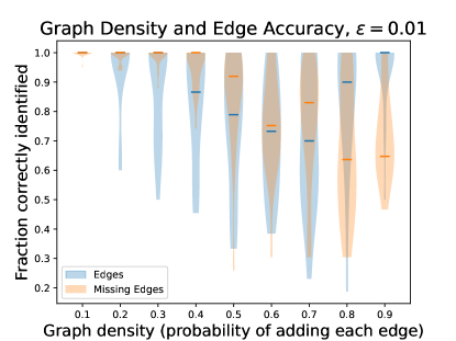
(a) (b)

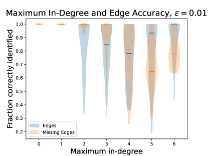
Figure 5: The results of Test 2. Horizontal ticks represent the median accuracy for recovering edges (blue) or lack of edges (orange). A violin plot is also shown, representing the density of results over 20 iterations at each value of $p$.

8 Discussion

The primary purpose of the results given here is a proof of identifiability, which gives hope for more efficient and practical algorithms in the future. Information theoretically, we have shown how the complexity of the visible variables (i.e. their cardinality), the sparsity of the graph structure, and the complexity of the global confounding (again, it’s cardinality) all interact within identifiability. Our proof suggests that the concepts of coarsening, immoral descendants, and false-positive edge detection may be crucial parts of future solutions.

In practice, the rank tests discussed here are data-intensive and suffer from instability in some settings. Future work should investigates alternatives to these tests, as well as options for continuous settings that can similarly leverage assumed limitations in the power of latent-class confounding.

Appendix A DEFERRED PROOFS

A.1 Proof of Lemma 2

Proof.

A key observation is that the moral graph of a subgraph of $\mathcal{G}$ has no additional edges relative to $\mathcal{G}^{(m)}$. That is, if $\mathcal{G}[\bm{W}]=(\bm{W},\bm{F})$ is a subgraph of $\mathcal{G}=(\bm{V},\bm{E})$ then the corresponding edge-sets of the moral graphs obey $\bm{F}^{(m)}\subseteq\bm{E}^{(m)}$ because adding vertices cannot have invalidated any previously contained immoralities.

Abbreviate $(\mathcal{G}[\operatorname{\mathbf{AN^{+}}}(\bm{S}\cup\bm{S}^{\prime}\cup\bm{C})])^{(m)}$ as $\mathcal{G}_{\bm{C}}^{(m)}$. Even though we do not know what $\bm{C}$ is, we know that the $1$-neighborhood of $\bm{S}$ in $\mathcal{G}_{\bm{C}}^{(m)}$ suffices as a separating set. $\mathcal{G}^{(m)}$ has all of the edges of $\mathcal{G}_{\bm{C}}^{(m)}$, so

$$\operatorname{\mathbf{NB}}_{1}^{\mathcal{G}_{\bm{C}}^{(m)}}(\bm{S})\subseteq\operatorname{\mathbf{NB}}_{1}^{\mathcal{G}^{(m)}}(\bm{S}).$$ (10)

Note that $\operatorname{\mathbf{NB}}_{1}^{\mathcal{G}^{(m)}}(\bm{S})$ is not necessarily a separating set for $\bm{S},\bm{S}^{\prime}$ in $\mathcal{G}^{(m)}$, in fact it may include some vertices in $\bm{S}$ itself. However, the size of the separating set is bounded by $\mathopen{|}\operatorname{\mathbf{NB}}_{1}^{\mathcal{G}^{(m)}}(\bm{S})\mathclose{|}$, which is no larger than $\mathopen{|}\bm{S}\mathclose{|}\Delta^{2}$. As we chose $\bm{S}$ arbitrarily, this bound also holds for $\bm{S}^{\prime}$. ∎

A.2 Proof of Lemma 5

Proof.

We will drop the conditioning on $\bm{c}$ in this proof for simplicity. Consider the sum

$$\sigma_{j}:=\sum_{i=1}^{j}\Pr(u_{i})\bm{\mathcal{M}}[X,Y\mid u_{i}],$$ (11)

and note that $\sigma_{k}=\bm{\mathcal{M}}[X,Y]$. Faithfulness with respect to $\mathcal{G}^{\prime}$ tells us that there is some assignment, which we call $u_{1}$ wlog, such that $X\not\perp\!\!\!\perp Y\mid u_{1}$. Hence ${\operatorname{rk}_{+}}(\sigma_{1})>1$.

Now, we show inductively that ${\operatorname{rk}_{+}}(\sigma_{i})={\operatorname{rk}_{+}}(\sigma_{i-1})+1$ is a measure $1$ event for $i=1,\ldots,k$. Denote $\bm{\mathcal{M}}[X,Y\mid u_{i}]=v_{i}w_{i}^{\top}$ with column space $v_{i}$ drawn from a subspace with non-zero measure on $\mathbb{R}^{n}$. The column space of $\sigma_{i-1}$ is rank $\leq i-1<m$, so it has measure zero on $\mathbb{R}^{m}$. Hence, $v_{i}$ being in the column space of $\sigma_{i-1}$ is a measure $0$ event. We conclude that ${\operatorname{rk}_{+}}(\sigma_{i-1}+\bm{\mathcal{M}}^{u_{i}}[X,Y])={\operatorname{rk}_{+}}(\sigma_{i-1})+1$ with measure $1$. Inducting on $i$ gives ${\operatorname{rk}_{+}}(\sigma_{k})>k$ with measure $1$. ∎

A.3 Proof of Lemma 14

Proof.

The algorithm designates vertices in $\bm{V}$ into the following sets and succeeds so long as those sets are disjoint.

1. $\bm{X}_{1}$ and $\bm{X}_{2}$

2. $\operatorname{\mathbf{NB}}_{2}(\bm{X}_{1}),\operatorname{\mathbf{NB}}_{2}(\bm{X}_{2})$

3. $\bm{T}_{ij}$

4. $\operatorname{\mathbf{NB}}_{1}(\bm{T}_{ij})$

$\mathopen{|}\bm{T}_{ij}\mathclose{|}\geq 2$ and $k\geq 2$, so the number of vertices added to $\bm{X}_{1},\bm{X}_{2}$ in the loop of Algorithm 2 is at most $\lceil\lg(2k+2-2)\rceil<\lg(k)+2$. To bound the $2$-neighborhood, we notice that we cannot easily apply our degree bound of $\Delta$ because $\bm{H}$ could be a clique in $\mathcal{G}_{1}$ (from FP edges). Instead, we bound

$$\mathopen{|}\operatorname{\mathbf{NB}}_{2}(\bm{X}_{1})\cup\operatorname{\mathbf{NB}}_{2}(\bm{X}_{2})\cup\bm{X}_{1}\cup\bm{X}_{2}\mathclose{|}\leq\Delta^{2}\mathopen{|}\bm{X}_{1}\cup\bm{X}_{2}\mathclose{|}+\Delta\mathopen{|}\bm{H}\mathclose{|}$$ (12)

because the distance $1$ neighborhood could include all of $\bm{H}$ but all additional neighborhoods are bounded by $\Delta$. $\mathopen{|}\bm{H}\mathclose{|}$ is $\mathcal{O}(\Delta^{2}\log(k))$ by Observation 2, so this bound is $\mathcal{O}(\Delta^{3}\log(k))$.

The size of $\bm{T}_{ij}$ is the largest when including $V_{i}$ or $V_{j}$ in $\bm{H}$, for which $\operatorname{\mathbf{NB}}_{1}(V_{i})$ could be all of $\bm{H}$ and $\operatorname{\mathbf{NB}}(V_{i})$ then necessarily falls outside of $\bm{H}$. This worst case gives

$$\mathopen{|}\bm{T}_{ij}\mathclose{|}\leq\mathopen{|}\bm{H}\mathclose{|}+\Delta^{2}.$$ (13)

which is $\mathcal{O}(\Delta^{2}\log(k))$. Expanding to the $1$ neighborhood picks up another factor of $\Delta$, bringing us again to $\mathcal{O}(\Delta^{3}\log(k))$.

∎

A.4 Proof of Lemma 8

Proof.

Suppose for contradiction that some vertex $B\in\operatorname{\mathbf{IMD}}(V_{i},V_{j})\cap\bm{S}^{+}_{j}$. $B\in\operatorname{\mathbf{IMD}}(V_{i},V_{j})$ implies that there is a directed path $\bm{P}\subseteq\operatorname{\mathbf{IMD}}(V_{i},V_{j})$ from $V_{i}$ to $B$. By the definition of an IPA, $B\in\bm{S}^{+}_{j}$ means that there must be some $\bm{C}$ with $B\perp\!\!\!\perp_{d}V_{i}\mid\bm{C}$. We conclude that $\bm{C}$ must contain some $C\in\bm{P}$ in order to block $\bm{P}$ from being an active path. However, this also means that $C\in\operatorname{\mathbf{IMD}}(V_{i},V_{j})$, which contradicts Observation 1. The same argument holds for $B\in\bm{S}_{i}^{+}$. ∎

A.5 Proof of Lemma 9

Proof.

We can form $\bm{S}_{i}^{+}$ out of $V_{i}$ and $\lceil\lg(k)\rceil$ arbitrary other vertices from $\bm{A}_{ij}$. Now, let the separating set be $\bm{C}:=\operatorname{\mathbf{MB}}^{\mathcal{G}[\bm{A}{ij}]}(\bm{S}_{i}^{+})$ and note that $\bm{C}$ d-separates $\bm{S}_{i}^{+}$ from all other elements of $\bm{A}_{ij}$. Since we know $\mathopen{|}C\mathclose{|}\leq\Delta^{2}(\lceil\lg(k)\rceil+1)$, we have at least $\lceil\lg(k)\rceil$ vertices in $\bm{A}_{ij}$ left to join with $V_{j}$ and make $\bm{S}_{j}^{+}$. ∎

A.6 Proof of Lemma 13

Proof.

The distance between $X\in\bm{X}$, and $V\in\bm{V}$ in $\mathcal{G}_{1}$ is less than or equal to the distance in $\mathcal{G}$, because $\bm{E}_{1}\supseteq\bm{E}$. This means that the $2$-neighborhood of $\bm{X}$ in $\mathcal{G}_{1}$ includes the $2$-neighborhood of $\bm{X}$ in $\mathcal{G}$. Furthermore because all vertices in $\operatorname{\mathbf{MB}}^{\mathcal{G}}(\bm{X})$ are distance $\leq 2$ from at least one $X\in\bm{X}$, we have that $\operatorname{\mathbf{MB}}^{\mathcal{G}}(\bm{X})$ is contained in the $2$-neighborhood of $\bm{X}$ in $\mathcal{G}_{1}$. ∎

A.7 Proof of Lemma 12

Proof.

$\bm{T}_{ij}$ contains both $\operatorname{\mathbf{PA}}(V_{i})$ and $\operatorname{\mathbf{PA}}(V_{j})$, so Lemma 1 tells us that we contain a separating set. ∎

A.8 Proof of Lemma 15

Proof.

Any two runs with assignments $\bm{d}_{ij}$ and $\bm{d}^{\prime}_{ij}$ that differ in their assignment to only one variable are alignable. Therefore, any two non-alignable runs can be aligned using a chain of Hamming-distance one alignments. ∎

References

- [1] Silvia Acid and Luis M De Campos “An algorithm for finding minimum d-separating sets in belief networks” In Proceedings of the Twelfth international conference on Uncertainty in artificial intelligence, 1996, pp. 3–10
- [2] Raj Agrawal, Chandler Squires, Neha Prasad and Caroline Uhler “The DeCAMFounder: nonlinear causal discovery in the presence of hidden variables” In Journal of the Royal Statistical Society Series B: Statistical Methodology, 2023, pp. qkad071 DOI: 10.1093/jrsssb/qkad071
- [3] A. Anandkumar, D. Hsu, F. Huang and S. M. Kakade “Learning high-dimensional mixtures of graphical models” In arXiv preprint arXiv:1203.0697, 2012
- [4] Ruichu Cai et al. “Causal Discovery with Latent Confounders Based on Higher-Order Cumulants” In arXiv preprint arXiv:2305.19582, 2023
- [5] K. Chaudhuri and S. Rao “Learning Mixtures of Product Distributions Using Correlations and Independence” In Proc. 21st Ann. Conf. on Learning Theory - COLT Omnipress, 2008, pp. 9–20 URL: http://colt2008.cs.helsinki.fi/papers/7-Chaudhuri.pdf
- [6] S. Chen and A. Moitra “Beyond the low-degree algorithm: mixtures of subcubes and their applications” In Proc. 51st Ann. ACM Symp. on Theory of Computing, 2019, pp. 869–880 DOI: 10.1145/3313276.3316375
- [7] 1000 Genomes Project Consortium “A global reference for human genetic variation” In Nature 526.7571 Nature Publishing Group, 2015, pp. 68
- [8] M. Cryan, L. Goldberg and P. Goldberg “Evolutionary trees can be learned in polynomial time in the two state general Markov model” In SIAM J. Comput. 31.2, 2001, pp. 375–397 DOI: 10.1137/S0097539798342496
- [9] S. Dasgupta “Learning mixtures of Gaussians” In Proc. 40th Ann. IEEE Symp. on Foundations of Computer Science, 1999, pp. 634–644
- [10] Jingqiu Ding et al. “Fast algorithm for overcomplete order-3 tensor decomposition” In Conference on Learning Theory, 2022, pp. 3741–3799 PMLR
- [11] J. A. Rhodes E. S. Allman “Identifiability of parameters in latent structure models with many observed variables” In Ann. Statist. 37.6A Institute of Mathematical Statistics, 2009, pp. 3099–3132 DOI: 10.1214/09-AOS689
- [12] J. Feldman, R. O’Donnell and R. A. Servedio “Learning Mixtures of Product Distributions over Discrete Domains” In SIAM J. Comput. 37.5, 2008, pp. 1536–1564 DOI: 10.1137/060670705
- [13] Y. Freund and Y. Mansour “Estimating a mixture of two product distributions” In Proc. 12th Ann. Conf. on Computational Learning Theory, 1999, pp. 53–62 DOI: 10.1145/307400.307412
- [14] Spencer L Gordon, Bijan Mazaheri, Yuval Rabani and Leonard J Schulman “Source Identification for Mixtures of Product Distributions” In Proc. 34th Ann. Conf. on Learning Theory - COLT 134, Proc. Machine Learning Research PMLR, 2021, pp. 2193–2216 URL: http://proceedings.mlr.press/v134/gordon21a.html
- [15] Spencer L Gordon, Bijan Mazaheri, Yuval Rabani and Leonard J Schulman “Causal Inference Despite Limited Global Confounding via Mixture Models” In 2nd Conference on Causal Learning and Reasoning, 2023
- [16] Spencer L Gordon et al. “Identification of Mixtures of Discrete Product Distributions in Near-Optimal Sample and Time Complexity” In arXiv preprint arXiv:2309.13993, 2023
- [17] M. Kearns et al. “On the learnability of discrete distributions” In Proc. 26th Ann. ACM Symp. on Theory of Computing, 1994, pp. 273–282 DOI: 10.1145/195058.195155
- [18] Joseph B Kruskal “Three-way arrays: rank and uniqueness of trilinear decompositions, with application to arithmetic complexity and statistics” In Linear algebra and its applications 18.2 Elsevier, 1977, pp. 95–138
- [19] Steffen L Lauritzen, A Philip Dawid, Birgitte N Larsen and H-G Leimer “Independence properties of directed Markov fields” In Networks 20.5 Wiley Online Library, 1990, pp. 491–505
- [20] Ankur Moitra “An almost optimal algorithm for computing nonnegative rank” In SIAM Journal on Computing 45.1 SIAM, 2016, pp. 156–173
- [21] Judea Pearl “Probabilistic reasoning in intelligent systems: networks of plausible inference” Morgan kaufmann, 1988
- [22] Judea Pearl “Causality” Cambridge university press, 2009
- [23] Yuval Rabani, Leonard J Schulman and Chaitanya Swamy “Learning mixtures of arbitrary distributions over large discrete domains” In Proc. 5th Conf. on Innovations in Theoretical Computer Science, 2014, pp. 207–224 DOI: 10.1145/2554797.2554818
- [24] Basil Saeed, Snigdha Panigrahi and Caroline Uhler “Causal structure discovery from distributions arising from mixtures of dags” In International Conference on Machine Learning, 2020, pp. 8336–8345 PMLR
- [25] Juergen Schmidhuber “Annotated History of Modern AI and Deep Learning” In arXiv preprint arXiv:2212.11279, 2022
- [26] P. Spirtes et al. “Constructing Bayesian network models of gene expression networks from microarray data” Carnegie Mellon University, 2000
- [27] Peter Spirtes “An Anytime Algorithm for Causal Inference” Reissued by PMLR on 31 March 2021. In Proceedings of the Eighth International Workshop on Artificial Intelligence and Statistics R3, Proceedings of Machine Learning Research PMLR, 2001, pp. 278–285 URL: https://proceedings.mlr.press/r3/spirtes01a.html
- [28] Peter Spirtes, Clark N Glymour and Richard Scheines “Causation, prediction, and search” MIT press, 2000
- [29] Peter Spirtes, C Meek and T Richardson “An algorithm for causal inference in the presence of latent variables and selection bias in computation, causation and discovery, 1999” MIT Press, 1999
- [30] Peter Spirtes et al. “Discovery algorithms for causally sufficient structures” In Causation, prediction, and search Springer, 1993, pp. 103–162
- [31] Chandler Squires and Caroline Uhler “Causal structure learning: A combinatorial perspective” In Foundations of Computational Mathematics 23.5 Springer, 2023, pp. 1781–1815
- [32] Kathie Y Sun et al. “A deep catalog of protein-coding variation in 985,830 individuals” In bioRxiv Cold Spring Harbor Laboratory, 2023, pp. 2023–05
- [33] B. Tahmasebi, S. A. Motahari and M. A. Maddah-Ali “On the Identifiability of Finite Mixtures of Finite Product Measures” (Also in “On the identifiability of parameters in the population stratification problem: A worst-case analysis,” Proc. ISIT’18 pp. 1051-1055), 2018 URL: https://arxiv.org/abs/1807.05444
- [34] Katarzyna Tomczak, Patrycja Czerwińska and Maciej Wiznerowicz “Review The Cancer Genome Atlas (TCGA): an immeasurable source of knowledge” In Contemporary Oncology/Współczesna Onkologia 2015.1 Termedia, 2015, pp. 68–77