Single-photon based Quantum Key Distribution and Random Number Generation schemes and their device-independent security analysis

Abstract

We present a single-photon based device-independent quantum key distribution scheme secure even against no-signaling eavesdropping, which covers quantum attacks, as well as ones beyond laws of physics but still obeying the rules for spatially separated events. The operational scheme is inspired by the Tan-Walls-Collett (1991) interferometric setup, which used the entangled state of two exit modes of a 50-50 beamsplitter resulting from a single photon entering one of its input ports, and weak homodyne measurements at two spatially separated measurement stations. The physics and non-classically of such an arrangement has been understood only recently. Our protocol links basic features of the first two emblematic protocols, BB84 and Ekert91, namely the random bits of the cryptographic key are obtained by measurements on single photon, while the security is positively tested if one observes a violation of a specific Bell inequality. The security analysis presented here is based on a decomposition of the correlations into extremal points of a no-signaling polytope which allows for identification of the optimal strategy for any eavesdropping constrained only by the no-signalling principle. For this strategy, the key rate is calculated, which is then connected with the violation of a specific Clauser-Horne inequality. We also adapt this analysis to propose a self-testing quantum random number generator.

Introduction

A single photon impinging on a 50-50 beamplitter is intuitively the quantum method to get random bits. Excitation of two spatially separated optical modes by just one single photon gives an entangled state of the modes. It seems to be the simplest physical situation in which Bell non-classical correlations could be observed. The trail blazing paper on this is the one of Tan, Wall and Collett [1], which was aimed at showing that one can obtain a Bell inequality violation via measurements at two spatially separated measuring stations, each observing one of the modes and performing weak homodyne measurements. This scheme thus far has not been used in quantum cryptography because of the controversies connected with it. The non-classicality of the Tan-Wall-Collett process was challenged by Santos [2], and finally excluded by an explicit local-realistic model of the correlations in [3].

In 1994 Hardy[4] showed a modified scheme, which is indeed non-classical, but involved a proper superposition of vacuum and single photon state impinging on the initial 50-50 beam-splitter, and worked effectively only up to probability of around 0.85 of finding the photon in the superposition, see [5]. Another unquestionable operational scheme involving beasmplitted single photons was put forward by Banaszek and Wodkiewicz [6], but it involved high intensity homodyning which was to give a displacement transformation. Various related scenarios were also proposed, e.g. in the cavity [7], with 3 single photons in quantum networks [8], with strong homodyne detection [9, 10] and the problem of non-classicality of beamsplitted single photon was also analyzed in the context of Gisin’s Theorem generalized to quantum fields [11]. Here we concentrate on all-optical setups aiming at revealing non-classicality due to single photon superposition in two modes. Thus we exclude operational situations in which the entanglement of optical modes is transferred into other systems, like in [12]. In papers [3],[13] and [5] a comprehensive analysis of the problem of non-classical effects induced by a single photon impinging on a 50-50 beamsplitter and homodyne measurements at spatially separated stations is presented. One of the conclusions of these is that non-classical effects leading to violations of Bell inequalities involve modified Tan-Walls-Collett setup, in which firstly homodyne measurements cannot be balanced, and secondly an on-off operation of the local oscillators defining the alternative settings of the observers during a Bell experiment is used (one of the crux ideas of Hardy’s paper). As this development allows one to finally think about quantum informational applications of such processes, we shall present here after further modifications to the setup two such applications and show that they have the status of device-independent protocols. Our modifications which include introduction of more experimentally friendly threshold detectors, instead of photon number resolving ones, and using stronger local oscillators (but still weak) allows us to obtain an order of magnitude higher violation of Bell inequality than the one presented in [13] and [5]. Thus, the modified process and protocol will lead to higher secure bit rates in quantum informational applications.

In this paper we show that a single photon impinged on a beamspliter and detected locally with weak-field homodyne measurement enables generation of random string of bits which can be further used in device independent key distribution protocol, secure against an eavesdropper which is not bounded by the laws of quantum physics. This line of research is being widely explored, in the presence of both the quantum adversary [14, 15, 16, 17, 18, 19] and also in the presence of a completely no-signalling eavesdropper [20, 21, 22, 23, 24] because of the great advantage of device-independent protocols. Namely, the intrinsic randomness of the generated bit string does not depend on trusted devices but relies solely on properties of the outcomes statistics. This can be tested with some Bell-type inequalities, which in our case is the Clauser-Horne (CH) inequality. Once the inequality is violated, the randomness is guaranteed independently of the physical realization of the experiment. Whereas to prove the security of randomness generation protocol it is enough to show the presence of true randomness in the bit string, proving security of key distribution requires studies of all possible eavesdropping attacks belonging to some class. In our analysis, we consider the most general no-signaling scenario and give the eavesdropper an ultimate power constrained only by basic rules of relativistic causality (no-signaling), to prepare any arbitrary probability distribution among herself, Alice and Bob. Here, we analyze the class of individual attacks. Next, the security of the protocol is proved by relating the lower bound on the raw secret key rate to the observed violation of the CH inequality.

Our proposal exhibits significant simplicity. Namely, one of the pair of settings that we use in CH inequality, see also [13], ensures perfect anti-correlations of local outputs. Thus, this pair of settings can serve for the generation of both: raw key and intrinsically random string of bits. We implement the entire protocol within the two-setting-two-outcome Bell-type scenario. As a result our system utilises the simplest set of bipartite conditional probability distributions $p(ab|xy)$, with $a,b,x,y\in\{0,1\}$, where $a,b$ denote the outcomes of Alice and Bob and $x$ and $y$ stand for their respective settings. Moreover, let us notice that our scheme links two emblematic protocols: BB84 and Ekert91. This is in the sense that the secret key is distributed by a single photon like in BB84. However, the security of the protocol is based on a Bell test as in Ekert91.

Results

Experimental Setup

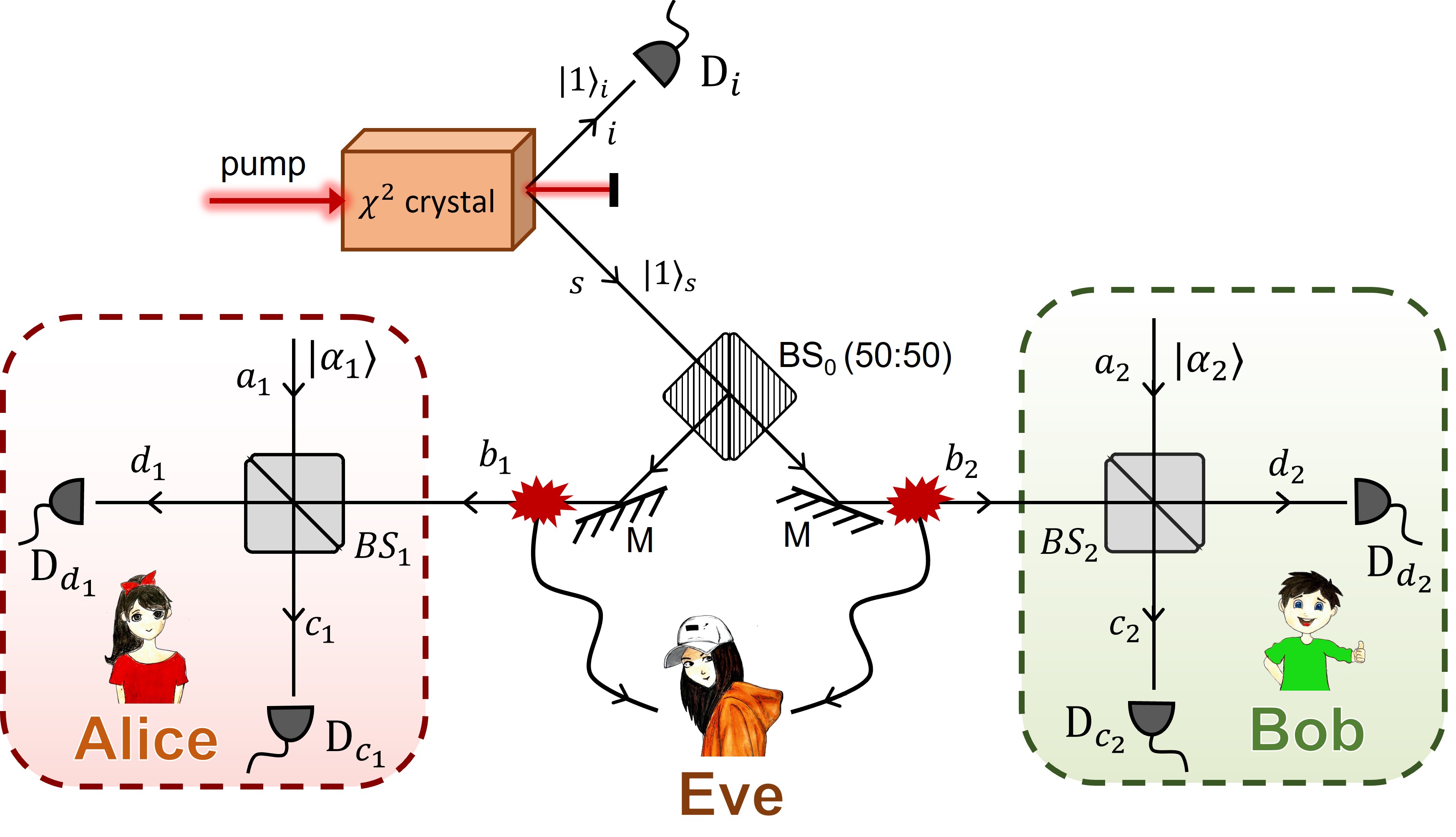
Figure 1: Schematic diagram of an all-optical setup for quantum key distribution protocol with a single photon based on a homodyne detection. The single photon produced in an SPDC process impinges on a balanced $(50:50)$ beamsplitter $BS_{0}$ with an additional phase shift $\tfrac{\pi}{2}$ and is sent to two spatially separated detection stations with two observers. Each of the measurement stations is equipped with a beamsplitter $(BS_{j})$ with tuneable transmitivity $T_{j}$ and with a local oscillator $\ket{\alpha}_{j}$ with tunable amplitude $\alpha_{j}$ for $j=1,2$. Both stations implement homodyne measurements. Alice and Bob choose their measurement settings by adjusting $T_{j}$ and $\alpha_{j}$ and collect data from single-photon detectors.

The scheme of the experimental setup is presented in the FIG. 1. Single photon is obtained from parametric down conversion with sufficiently weak amplification gain (’pump’), such that the state emitted in the process is practically a superposition of vacuum and a photon pair. The detector is placed in the idler mode $i$, which announces the appearance of a photon, making our experiment event-ready. Further on, only runs with detected idler photon are taken into consideration. This detection marks a successful run of the device. The heralded in this way single photon from the signal mode $s$ impinges on a balanced beamsplitter $BS_{0}$. The resulting output field is distributed into two spatially separated measurement stations of Alice and Bob. The state of the output modes of the beamsplitter $BS_{0}$ which plays a role of the input state for Alice and Bob

$$\ket{\psi}_{b_{1},b_{2}}=\frac{1}{\sqrt{2}}(\hat{b}_{1}^{\dagger}+\hat{b}_{2}^{\dagger})\ket{\Omega}=\frac{1}{\sqrt{2}}(\ket{01}_{b_{1},b_{2}}+\ket{10}_{b_{1},b_{2}}),$$ (1)

where $\ket{\Omega}$ is the vacuum state, and $\hat{b}_{j}^{\dagger}$, denotes the creation operator in the mode $b_{j}$, for $j=1,2$. The modes $b_{1}$ and $b_{2}$ are transferred, respectively, to Alice and Bob. They perform homodyne measurements, the settings of which are chosen by tuning the transmitivity $T_{j}$ of their beamsplitters $BS_{j}$ and the amplitude $\alpha_{j}$ of local oscillators fed in the modes $a_{j}$. The unitary transformation related to $BS_{j}$ transforms the input modes $a_{j}$ and $b_{j}$ into the output modes $c_{j}$ and $d_{j}$ upon which the photodetection is then performed by the local detectors. We stress that any type of detector that is able to detect single photon can be used in this experiment, even the simplest binary avalanche photo detector with enough sensitivity.

Cryptographic Protocol

Our cryptographic scheme is based on a Bell-type scenario. The local oscillators’ amplitudes are equal $\alpha_{1}=\alpha_{2}=\alpha$ and the transmitivity $T$ of beamsplitters $BS_{j}$ is optimized in order to maximize violation of a Bell inequality described further in the text. Alice and Bob randomly choose between two possible measurement settings: $\{on,\ off\}$. For on setting the local oscillators are switched on i.e. $\alpha\neq 0$. For off setting local oscillator is turned off i.e. $\alpha=0$. Note that the transmitivity of the local beamsplitters $BS_{j}$ is fixed. The setting change requires only blocking the local oscillator, which could be easily realized e. g. with shutter. This feature is an additional advantage from the point of view of experimental feasibility.

After each run of the experiment, both parties assign binary outcomes $\{0,1\}$ related to the number of photons $n_{c_{j}}$ and $n_{d_{j}}$ measured in their local detectors. The assignment depends on the chosen settings and goes in the following way: $\\ \text{for {on} setting}:\left\{\begin{array}[]{ll}0:&\mbox{if at least one photon is detected in the mode $d_{j}$ and no photons in mode $c_{j}$ \ i.e. \ }(n_{d_{j}}>0\wedge n_{c_{j}}=0)\\ 1:&\mbox{ for all other events }\end{array}\right.\\ \text{for {off} setting}:\left\{\begin{array}[]{ll}0:&\mbox{if any photon is detected \ i.e. \ }(n_{d_{j}}>0\vee n_{c_{j}}>0)\\ 1:&\mbox{for all other events }\end{array}\right.$

Note that such an assignment is perfectly tailored for the use of binary photodetectors and leads to the following conditional probability distributions $P^{\alpha,T}_{AB}(ab|xy)$ in which $a$ and $b\in\{0,1\}$ and $x$ and $y\in\{on,\ off\}$ for $\alpha$ and $T$:

$$P^{\alpha,T}_{AB}(ab|xy)=\begin{array}[]{cc|cc|cc}&\lx@intercol\hfil x\hfil\lx@intercol&\lx@intercol\hfil off\hfil\lx@intercol&\lx@intercol\hfil on\hfil\lx@intercol\\ y&\text{\diagbox[width=22.0pt,height=22.0pt,innerrightsep=0.0pt]{{\shortstack[l]{$b\,\,\,\,\,\,$}}}{{\shortstack[r]{$a\,\,\,$}}}{}}&0&1&0&1\\ \hline\cr\\[-8.99994pt] \hbox{\multirowsetup$off$ }&0&0&\frac{1}{2}&\xi_{00}&\xi_{01}\\[3.00003pt] &1&\frac{1}{2}&0&\xi_{10}&\xi_{11}\\[1.99997pt] \hline\cr\\[-8.99994pt] \hbox{\multirowsetup$on$ }&0&\xi_{00}&\xi_{10}&\beta_{00}&\beta\\[3.00003pt] &1&\leavevmode\nobreak\ \leavevmode\nobreak\ \xi_{01}\nobreak\leavevmode\nobreak\leavevmode&\leavevmode\nobreak\ \leavevmode\nobreak\ \xi_{11}\nobreak\leavevmode\nobreak\leavevmode&\leavevmode\nobreak\ \leavevmode\nobreak\ \beta\nobreak\leavevmode\nobreak\leavevmode&\leavevmode\nobreak\ \leavevmode\nobreak\ \beta_{11}\nobreak\leavevmode\nobreak\leavevmode\end{array},\leavevmode\nobreak\ \leavevmode\nobreak\ \leavevmode\nobreak\ \leavevmode\nobreak\$$ (10)

where the exact forms of $\xi_{q},\,\beta_{q}$ are given in the Supplementary information A.

It is clearly noticeable that for (off, off) we observe perfect anti-correlations as only a single photon from the signal beam is present in the system and detection of the photon can occur only in one of the measurement stations. Thus, the outcomes from runs (off, off) will be used for generation of a secret raw key. A part of the (off, off) outcomes will be used ( together with the results obtained from the three other possible choices of settings) to perform CH inequality Bell test. The test is done to check the security of the distributed secret key. In order to ensure that the secret raw key is long enough Alice and Bob should choose off setting more often than on.

When the experiment is done, Alice reveals to Bob all her settings and the results, which are needed to perform a Bell test or in general to perform a search for eavesdropper optimal strategy, i.e. all on and the part of off results. These results combined with Bob’s local ones allow Bob to estimate the key rate and to perform standard privacy amplification procedures. For the scheme described above the following CH inequality will be used:

$$\begin{split}-1\leq CH=P(00|on,on)+P(00|on,off)+P(00|off,on)-P(00|off,off)-P_{A}(0|on)-P_{B}(0|on)\leq 0.\end{split}$$ (11)

Inequality (11) can be violated for some value of $\alpha$ given an optimized value of $T$. FIG. 2 shows how the maximal value of the CH expression in (11) increases as a function of the square of the amplitude $\alpha^{2}$. To assess maximal violation, we consider the limiting case of $\alpha\rightarrow\infty$, with the constraint that the product $\alpha^{2}T$ converges to a finite value, i.e. $\alpha^{2}T\rightarrow k$. Then the limiting value of the $CH$ expression is given by:

$$\lim_{\alpha^{2}\rightarrow\infty}\lim_{\alpha^{2}T\rightarrow k}CH=e^{-2k}\left(2-e^{k}\right)k,$$ (12)

and it reaches maximal value of $CH\approx 0.1086$ for $k\approx 0.260$. Looking at the Fig. 2 one notices that in practice the CH value saturates rapidly as a function of $\alpha^{2}$ and one is close to the maximal violation already for $\alpha^{2}\approx 10$.

To sum up, we present short outline of the protocol:

1. Alice and Bob agree on the choice of the local oscillators’ amplitude $\alpha$ and with respect to it they set local beamsplitters’ transmittivity $T$, so that the violation of CH inequality is possible for the setup.

2. Single photon pairs are generated in PDC process. When the detector placed in the idler mode clicks, Alice and Bob start the measurement with one of the local settings chosen by each of them. The choice between the settings on and off is random and with no previous agreement between the parties. However, there should be sufficiently more off than on choices, as off settings are used to test the security as well as to generate the raw key.

3. The signal photon impinges on the balanced beamsplitter and the resulting output field is sent to the detection station of Alice and Bob.

4. At the detection stations local homodyne measurement is performed.

5. After sufficient number of experimental runs Alice communicates her settings and the part of her results needed for Bell test to Bob, who performs the Bell test (or in general performs search for eavesdropper optimal strategy) and privacy amplification. If inequality is not violated, Bob terminates the key sharing procedure.

6. Raw key is obtained from a fraction of runs of the experiment in which local settings where set to (off, off).

Outline of security proof.

Our security proof assumes that Eve has full control over the preparation of the physical system that mediates and imitates the correlations between Alice and Bob. The entire system is described in terms of joint no-signalling probability distributions. This is the most general approach to tackle the question of security, as any protocol which is secure against individual attacks by no-signaling Eve is also secure against any individual attacks of Eve able to control quantum resources used by Alice and Bob.

The clue of the proof is the mathematical property of no-signalling correlations, which is that whenever in a tripartite scenario a Bell inequality violation is observed between two parties (Alice and Bob), the third party (Eve), who governs the process of preparation of the correlations cannot have deterministic knowledge about all the outcomes of Alice and Bob. The degree of Eve’s uncertainty about Alice and Bob’s outcomes can be directly expressed in terms of the degree of violation of a Bell inequality. In order to do it, we utilize the theory of decomposition of non-signalling distributions into mixtures consisting of either fully deterministic correlations or maximally non-local (but still non-signalling) correlations, for which the local outcomes are totally random. By means of recent developments in this theory we find a distribution which for a given value of a Bell inequality violation observed by Alice and Bob ensures a minimal amount of admixture of non-local correlations in the decomposition. Such a strategy is an optimal one for Eve, who in this way minimizes the privacy of Alice and Bob’s outcomes. Based on this minimal amount of privacy, we find a lower bound on the secret key rate generated between Alice and Bob as a function of observed Bell inequality violation.

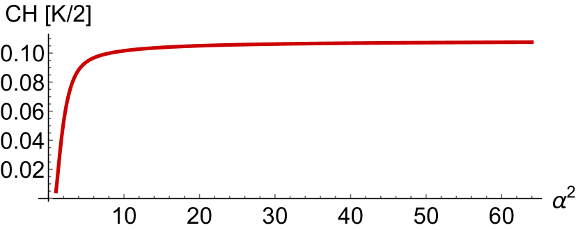
Figure 2: Plot of the optimal violation of the right hand side of the Clauser-Horne inequality, given in (11), as a function of the local oscillator strength $\alpha^{2}$, for state $\ket{\psi}_{b_{1},b_{2}}$. The value of the CH expression is optimized with respect to the beamsplitter transmissivity $T$ for each value of $\alpha^{2}$ and it determines the value of the secret key rate by the formula $K=2CH$.

Security

To prove security of our protocol let us introduce eavesdropper (Eve) into the system. We consider the presence of no-signaling Eve which has full control over the state preparation and performs individual attacks in each run of the protocol.

In each run, Eve prepares a tripartite system from which two subsystems are distributed to Alice and Bob, and the third subsystem is kept by her. Afterwards Eve can choose some measurement from set $Z\equiv\{z\}$ to perform on her subsystem which results in some outcome $e$ used by her to extract information. We assume that the probability distribution $\tilde{P}(abe|xyz)$ of the extended system is no-signaling i.e. it fulfils no-signaling conditions:

$$\sum_{e}\tilde{P}(abe|xyz)=P(ab|xy),\leavevmode\nobreak\ \leavevmode\nobreak\ \forall z\in Z$$ (13)

and analogous conditions for Alice and Bob. This corresponds to statement that the non-signalling Eve cannot influence the statistics of outcomes of the honest parties through her choices of the measurement settings. What is more, Eve is able to prepare the system in such a way that she can achieve any $\tilde{P}(abe|xyz)$ that ideally mimics the quantum device assumed by Alice and Bob characterized by probability distribution $P^{\alpha,T}_{AB}(ab|xy)$ (10) to avoid exposing of herself. Note that $P^{\alpha,T}_{AB}(ab|xy)$, as a quantum probability distribution, is by definition no-signaling between the parties. Such an eavesdropper can be restated in terms of the theory of no-signaling correlations as Eve holding complete extension[25] of quantum device $P^{\alpha,T}_{AB}(ab|xy)$. Complete extension is a generalization of the purification of the quantum state into no-signaling correlation boxes. This gives ultimate power to no-signaling Eve for individual attacks in the same sense as using purification by quantum Eve is optimal. For more details on theory of complete extensions see Supplementary information B or for a full discussion [25].

Secret key rate

In order to calculate secret key rate we have to find an optimal strategy for Eve. Let us consider the strategy in which Eve decomposes the no-signaling correlation box $P^{\alpha,T}_{AB}(ab|xy)$ into the extremal points of the no-signaling polytope corresponding to a scenario with two inputs and two outputs per party. By extremal points we mean those that cannot be written as a convex combination of other points from the correlation polytope. It is known that this polytope contains $24$ extremal points among which $16$ are local boxes and $8$ are non-local boxes. They are characterised by respectively four and three binary indices, and their formal definitions are provided in the Methods section in formulas (47) and (48). Here let us recall for example local box $L_{0011}$ and non-local box $B_{111}$:

$$L_{0011}=\begin{array}[]{cc|cc|cc}&\lx@intercol\hfil x\hfil\lx@intercol&\lx@intercol\hfil off\hfil\lx@intercol&\lx@intercol\hfil on\hfil\lx@intercol\\ y&\text{\diagbox[width=22.0pt,height=22.0pt,innerrightsep=0.0pt]{{\shortstack[l]{$b\,\,\,\,\,\,$}}}{{\shortstack[r]{$a\,\,\,$}}}{}}&0&1&0&1\\ \hline\cr\\[-8.99994pt] \hbox{\multirowsetup$off$ }&0&0&0&0&0\\[3.00003pt] &1&1&0&1&0\\[1.99997pt] \hline\cr\\[-8.99994pt] \hbox{\multirowsetup$on$ }&0&1&0&1&0\\[3.00003pt] &1&\leavevmode\nobreak\ \leavevmode\nobreak\ 0\nobreak\leavevmode\nobreak\leavevmode&\leavevmode\nobreak\ \leavevmode\nobreak\ 0\nobreak\leavevmode\nobreak\leavevmode&\leavevmode\nobreak\ \leavevmode\nobreak\ 0\nobreak\leavevmode\nobreak\leavevmode&\leavevmode\nobreak\ \leavevmode\nobreak\ 0\nobreak\leavevmode\nobreak\leavevmode\end{array},\leavevmode\nobreak\ \leavevmode\nobreak\ \leavevmode\nobreak\ \leavevmode\nobreak\ \,\,\,\,\,\,\,B_{111}=\begin{array}[]{cc|cc|cc}&\lx@intercol\hfil x\hfil\lx@intercol&\lx@intercol\hfil off\hfil\lx@intercol&\lx@intercol\hfil on\hfil\lx@intercol\\ y&\text{\diagbox[width=22.0pt,height=22.0pt,innerrightsep=0.0pt]{{\shortstack[l]{$b\,\,\,\,\,\,$}}}{{\shortstack[r]{$a\,\,\,$}}}{}}&0&1&0&1\\ \hline\cr\\[-8.99994pt] \hbox{\multirowsetup$off$ }&0&0&\frac{1}{2}&\frac{1}{2}&0\\[3.00003pt] &1&\frac{1}{2}&0&0&\frac{1}{2}\\[1.99997pt] \hline\cr\\[-8.99994pt] \hbox{\multirowsetup$on$ }&0&\frac{1}{2}&0&\frac{1}{2}&0\\[3.00003pt] &1&\leavevmode\nobreak\ \leavevmode\nobreak\ 0\nobreak\leavevmode\nobreak\leavevmode&\leavevmode\nobreak\ \leavevmode\nobreak\ \frac{1}{2}\nobreak\leavevmode\nobreak\leavevmode&\leavevmode\nobreak\ \leavevmode\nobreak\ 0\nobreak\leavevmode&\leavevmode\nobreak\ \leavevmode\nobreak\ \frac{1}{2}\nobreak\leavevmode\nobreak\leavevmode\end{array}.$$ (30)

Based on the Carathéodory theorem [26, 27] each of the element (box) in the polytope can be decomposed at most into $9$ extremal boxes [25]. The weights with which particular boxes appear in the decomposition can be simply interpreted as the probabilities that Eve prepares the subsystem of Alice and Bob in such a way that it exactly matches correlations of particular extremal box. Such decompositions are called minimal ensembles if one cannot find another decomposition using only a subset of extremal boxes used in a given decomposition. Note that there is always finite number of such ensembles. What is more they can be easily and efficiently calculated using pseudo-inverse. Eve after preparing some minimal ensemble performs measurement on her subsystem to reveal which no-signaling box was shared with Alice and Bob. If the shared box is local, Eve gains perfect deterministic knowledge about the results of the run. However, if the box is non-local, she has zero knowledge about results for key generation runs, as for this case they are completely random (see for example (30)).

The key feature of the strategy is that Eve as an input chooses which minimal ensemble to prepare is that Eve can effectively reach any decomposition of $P^{\alpha,T}_{AB}(ab|xy)$ in terms of any points in no-signaling polytope by properly using input randomizer and output post-processing channel i.e. she can perform any no-signaling strategy for individual attacks. Note that, post-processing channel due to the data-processing inequality cannot improve mutual information between Bob and Eve or Alice and Eve [28]. Therefore any strategy using post-processing channel cannot be more optimal, and we can focus on input randomization. In Supplementary information C we provide the set of all minimal ensembles for $P^{\alpha,T}_{AB}(ab|xy)$ for a pair of settings $\{\alpha,T\}$ that provide near optimal violation of CH inequality (11), namely for $\alpha\rightarrow\infty$ and $T$ such that $\alpha^{2}T$ tends to some finite number $k$. We stress that we find analogous ensembles for all $\alpha$ considered on Figure 2 with only slightly changed probabilities. Among those minimal ensembles there is one, which we denote as $\mathbf{M_{op}}$ that has the smallest total probability of Eve sending non-local boxes $p_{nl}$. Note that $p_{nl}\neq 0$ is provided by the violation of CH inequality. As Eve wants to perform optimally she has to minimize the probability of non-local boxes as these do not give her any information. Therefore, optimal Eve will always choose the setting corresponding to ensemble $\mathbf{M_{op}}$ as otherwise she will introduce more randomness to her results, i.e. she would more often have to guess the bit as non-local boxes would appear with higher frequency.

Knowing optimal strategy we can calculate secret key rate for one way communication using Csiszár-Körner formula [29]:

$$K=max\{I(A:B)-I(A:E),I(A:B)-I(B:E)\},$$ (31)

where $I(X:Y)$ stands for mutual information. Due to the perfect anti-correlation between Alice and Bob for key generation runs we have $I(A:B)=1$. Further, due to the symmetry of our setup, we have $I(B:E)=I(A:E)$. What is more, as Eve gets perfect knowledge from local boxes, mutual information between Bob and Eve is simply equal to the probability of sending local box by Eve $p_{l}=1-p_{nl}$. Finally, the key rate is given just as $K=p_{nl}$. In the Methods section we show based on Eve optimal strategy that there is the following relation between the key rate and CH inequality violation:

$$K=2CH.$$ (32)

Based on FIG 2 we observe that with growing $\alpha$ the key rate grows to its optimal value $K\approx 0.217$ for $\alpha\rightarrow\infty$ which can be found based on eq. (12). However, the maximal key rate is quickly saturated and already for $\alpha^{2}=8$ the key rate is $K\approx 0.2$. What is important is that the use of such $\alpha$ is experimentally feasible. Note that, optimal strategy for Eve in principle can vary if one introduces different noise structures, and therefore relation (32) is not necessarily general. However, in such a case, one can still use algorithm for finding the optimal strategy for Eve through minimal ensembles to calculate the key rate for his specific correlation box.

Self-testing random number generator

Our proposed experimental setup can also be used as a self-testing random number generator (RNG) [30]. In this context, the task of the protocol is to generate provably random bits, without the need for perfect correlation between bits possessed by Alice and Bob, as in the case of secret key generation. The RNG protocol itself is exactly the same as for key distribution, what is different is the role played by non-classical correlations and the security proof. In the case of QKD correlations shared between Alice and Bob play double role: first for assuring perfect correlations between shared random bits, second for testing security of the protocol by measuring Bell inequality violation. In the case of RNG protocol, the only role of shared correlations between Alice and Bob is to test the security of the RNG protocol, also by measuring Bell inequality violation.

Let us first present the general idea of device-independent security proof of RNG protocol (see [31], sec. IV.C.3). The main entity in the proof is the average probability of Eve guessing Alice’s outcome (in this presentation we focus on Alice’s device as the RNG source, whereas Bob’s device serves just for obtaining Bell inequality violation; due to symmetry of our scenario the roles of Alice and Bob can be exchanged without any modification). Let us assume, as in the previous case, that Alice, Bob and Eve share joint correlations $\tilde{P}(abe|xyz)$ prepared by Eve of any nature, with the only restriction that they are no-signalling (13). Then the average guessing probability can be defined using reduced conditional probability distributions [31]:

$$p_{\textrm{guess}}=\max_{z}\sum_{e}P(e|z)\max_{a}P(a|e,z).$$ (33)

We assume that Alice and Bob perform a Bell test, which leads to the experimental estimation of an expression $\mathcal{B}$ of some Bell inequality. In specific scenarios, in particular ours, guessing probability can be expressed as a function of the Bell value $\mathcal{B}$: $p_{\textrm{guess}}=p_{\textrm{guess}}(\mathcal{B})$. The next step of the proof is introduction of the so-called min-entropy, which measures the randomness of a discrete random variable in the strictest way among all entropies defined within the family of Renyi entropies [32]. The mean entropy is defined as the minus logarithm of the most probable outcome, which in the context of our problem translates to:

$$H_{\textrm{min}}(\mathcal{B})=-\log_{2}\left(p_{\textrm{guess}}(\mathcal{B})\right).$$ (34)

Min-entropy in our case can be treated as a function of the Bell value $\mathcal{B}$, which will be crucial in our argumentation. $H_{\textrm{min}}$ well approximates the maximal number of securely random bits per run of the protocol that can be extracted from raw data in a given protocol using optimal privacy amplification techniques (known in this context as randomness extraction techniques) [33, 32]:

$$l_{\textrm{random}}\approx H_{\textrm{min}}.$$ (35)

As was shown in fundamental works on quantum randomness generation [34, 35, 36], this relation holds also in the quantum scenario, namely if all the correlations are due to sharing quantum states. Therefore, in device-independent schemes for quantum random number generation, the number of securely random bits in a given protocol involving the Bell inequality test is a function of the measured Bell value $\mathcal{B}$:

$$l_{\textrm{random}}\approx-\log_{2}\left(p_{\textrm{guess}}(\mathcal{B})\right).$$ (36)

Let us now apply the above presented proof to the case of our protocol. We will utilize the super-quantum no-signalling description of correlations used in the previous sections. Although there are no known results on the precise relation between the number of secure bits and entropy in the case of such general model of correlations, the relation (35) calculated for the general no-signalling distribution gives the lower bound for the number of extractable random bits in the case of quantum correlations, since they are no-signalling. More precisely, the relation (35) for no-signalling correlations gives the minimal number of extractable random bits for any quantum implementation of the ideal individual eavesdropping attack. To calculate this number, let us first calculate the guessing probability (33). In the model of Eve preparing arbitrary non-signalling distribution the guessing probability of Alice’s (or Bob’s) outcome does not depend on Alice’s (or Bob’s) settings. As in the case of key rate analysis we can assume without loss of generality that Eve prepares some minimal ensamble of extremal boxes. Then there are just two possibilities for guessing probability. If Eve’s outcome indicates that a local box has been prepared, the guessing probability equals $1$, as this case is fully deterministic, whereas if non-local box has been prepared, the guessing probability equals $\tfrac{1}{2}$, since the outputs are then totally random. Therefore, guessing probability for Eve equals:

$$p_{\textrm{guess}}=p_{l}+\frac{1}{2}p_{nl}=1-\frac{1}{2}p_{nl},$$ (37)

where the second equality comes just from normalisation $p_{l}+p_{nl}=1$. Now note that $p_{\textrm{guess}}$ (37) is maximized for minimal $p_{nl}$, therefore, it attains maximal value for the same optimal decomposition $\mathbf{M_{op}}$ as discussed in the case of optimal Eve’s attack against secret key generation. We already know that for this decomposition, the probability $p_{nl}$ is equal to twice the $CH$ value: $p_{nl}=2CH$, therefore we finally have:

$$p_{\textrm{guess}}=1-CH.$$ (38)

This gives the approximate number of truly random bits that can be extracted when using our protocol:

$$l_{\textrm{random}}\approx-\log_{2}\left(1-CH)\right).$$ (39)

For the maximal violation $CH\approx 0.1086$ we obtain $l_{\textrm{random}}\approx 0.1660$.

Discussion

In summary, we have proposed a device-independent cryptographic scheme secure against non-signaling Eve. Our protocol lies in between the famous BB84 and Ekert91 protocols as the secret key is distributed using a single photon interacting with a beamsplitter and the security is based upon observed Bell non-classicality, however, this nonclassicality is induced by the single-photon superposition in two modes rather than by the presence of entanglement between two particles. The advantage of our protocol is that it requires the minimal number of settings for performing a Bell test and additionally uses just one of those settings in the process of key generation whereas the previous protocols had to add an additional setting for the key generation. This allows for the security analysis in terms of the simplest non-signaling polytope and thus the least computationally demanding security check against no-signaling eavesdropping, which can be important for smooth and fast operations of potential commercial devices based on such solutions. The security analysis is based on a search for the optimal strategy for Eve through the decomposition of obtained correlations to extremal points of the no-signaling polytope. The method used is independent of the construction of the device and could also be applied in different scenarios, for example, in the analysis of the proposed setup in the presence of noise. We also apply this method to propose the scheme for quantum random number generation. The obtained probability of guessing the bit by the third parties allows us to compute lower bounds for the bitrate. This shows the versatility of the analysis used.

It is important to notice that while the security analysis method based on the correlations decomposition is independent of the device, a relation between the violation of a specific CH inequality with the key rate and bit rate obtained by the decomposition of correlations is device dependent, and these relations do not have to be general. This is because the relations for the violation of CH inequality were calculated for a specific class of correlations present in the perfect implementation of the proposed experimental setup, and while it could hold in the noisy scenario it is not guaranteed. The presence of noise in correlations could result in a different decomposition of the correlations being optimal for Eve, potentially resulting in different relations of key rate and bit rate with the used CH inequality. Thus, to obtain unconditional security and accurately calculate key rate or bit rate one should apply the whole decomposition procedure, but still one can treat CH inequality violation as a quick estimate if the security was not compromised beforehand. This is because obtaining a violation of some Bell inequality is a necessary condition for obtaining a nonzero key rate and bit rate. The violation of CH inequality can also be used for device calibration, as the higher violation of CH inequality indicates a more significant presence of not favorable for Eve non-local correlations, which results in higher key rate and bit rate. Still, further developments of the protocol in terms of noisy systems may provide a general proof of the relation between the violation of the CH inequality and the key rate.

The proposed experimental setup should be possible to implement in the laboratory with current technology, as it requires only standard quantum optical equipment and high-efficiency threshold single-photon detectors, which are commercially available. Furthermore, the measurement itself in its principles is a homodyne measurement, which has been used in laboratories for decades with the difference that used local oscillator fields are weak. Still, experiments involving such techniques were successfully conducted in recent years [37].

Finally, note that arbitrary no-signalling correlations are impossible to observe or engineer. Still they allow to construct simple criteria for secure transmission by modeling on eavesdropper constrained only by the rules of special relativity. Therefore, even though our method is highly general and computationally not demanding, one could opt to consider only quantum strategies for eavesdropping. Because a set of quantum correlations is a subset of a set of no-signaling correlations, such an approach results in at least as high key rate as for no-signaling Eve and therefore could provide faster key distribution without real compromises on security. However, analyzing of all possible quantum strategies is a demanding problem worthy of further investigation, even in this simplest possible set of configurations. One can also try to provide security only in some subclasses of quantum eavesdropping strategies specific to the device that are most probable to be implemented; however, this is a non-trivial research problem as the considered system is infinite-dimensional.

Methods

Probabilities for all versus nothing events

In this section, we show how probabilities $P^{\alpha,T}_{AB}(ab|xy)$ can be calculated. To simplify the problem, let us restate measurement setting off for both the parties in such a way that it corresponds to removing of the beam splitter $BS_{j}$ (which is equivalent to the situation of a beamsplitter of $100\%$ transmitivity) and outcomes $0$ and $1$ are assigned as in the case of on setting. One can easily check that such scenario is exactly equivalent to the one described in the main text.

We consider the following state:

$$\ket{\psi(\alpha,\phi)}=\frac{1}{\sqrt{2}}\ket{\alpha e^{i\phi}}_{a_{1}}\left(\ket{01}_{b_{1},b_{2}}+\ket{10}_{b_{1},b_{2}}\right)\ket{\alpha e^{i\phi}}_{a_{2}},$$ (40)

where for off setting $\alpha=0$. The probability of measuring specific combination of photons in modes $d_{i},c_{i}$ is given by:

$$P(k,l,n,m|x,y)=|_{c_{1},d_{1},c_{2},d_{2}}\bra{k,l,n,m}\hat{U}_{1}(x)\hat{U}_{2}(y)\ket{\psi(\alpha,\phi)}|^{2},$$ (41)

where $\hat{U}_{i}(x)$ denotes unitary operator corresponding to the beamsplitter $BS_{i}$ acting on the $i$-th party for setting $x$. This unitary performs the following transformation of annihilation operators for on setting:

$$\left(\begin{array}[]{c}\hat{c}_{j}\\ \hat{d}_{j}\end{array}\right)=\left(\begin{array}[]{cc}\cos{\chi}&i\sin{\chi}\\ i\sin{\chi}&\cos{\chi}\end{array}\right)\left(\begin{array}[]{c}\hat{a}_{j}\\ \hat{b}_{j}\end{array}\right)$$ (42)

where $\chi=\cos^{-1}(\sqrt{T})$. For off setting we have $\hat{U}_{i}(off)=\mathbb{I}$. Based on that, probabilities $P^{\alpha,T}_{AB}(ab|xy)$ can be calculated as:

$$P(00|x,y)=\sum_{l=0}^{\infty}\sum_{m=0}^{\infty}P(0,l,0,m|x,y),$$ (43)

$$P(10|x,y)=\sum_{k=1}^{\infty}\sum_{l=0}^{\infty}\sum_{m=0}^{\infty}P(k,l,0,m|x,y)+\sum_{m=0}^{\infty}P(0,0,0,m|x,y),$$ (44)

$$P(01|x,y)=\sum_{l=0}^{\infty}\sum_{n=1}^{\infty}\sum_{m=0}^{\infty}P(0,l,n,m|x,y)+\sum_{l=0}^{\infty}P(0,l,0,0|x,y),$$ (45)

$$P(11|x,y)=1-P(00|x,y)-P(10|x,y)-P(01|x,y).$$ (46)

Explicit expressions for those probabilities are provided in Supplementary Information B.

Finding minimal ensembles

Here we present how one can find a minimal ensemble for some no-signalling correlation box for two-input-two-output scenario. For such a case there are 24 extremal points in the no-signalling polytope. They can be characterised in the following way: 16 local boxes:

$$\mathrm{L}_{qrst}(ab|xy)=\left\{\begin{array}[]{cc}1&\mbox{if $a=qx\oplus r$,}\\ &\leavevmode\nobreak\ \leavevmode\nobreak\ \leavevmode\nobreak\ \mbox{$b=sy\oplus t$}\\ 0&\mbox{otherwise}.\end{array}\right.$$ (47)

with $q,r,s,t\in\{0,1\}$ and $x,y=0$ for off setting and $x,y=1$ for on setting. Remaining $8$ non-local boxes can be put as:

$$\mathrm{B}_{rst}(ab|xy)=\left\{\begin{array}[]{ll}1/2&\mbox{if $a\oplus b=xy\oplus rx\oplus sy\oplus t$}\\ 0&\mbox{otherwise}.\end{array}\right.$$ (48)

In order to find all minimal ensembles one can treat correlation box as a matrix which we denote as $\mathbb{P}(ab|xy)$. Now, let us choose some subset $\mathcal{I}_{s}$ of the set of indices $\mathcal{I}=\{1,...,24\}$ with power of this subset $\overline{\mathcal{I}_{s}}\leq 9$. The reason for choosing the maximal power of the set is that each point in the regarded polytope can be decomposed at most using $9$ extremal points. The assumed decomposition can be written using those extremal boxes $\texttt{E}^{i}$ in the form of a matrix from the set of all extremal boxes $\{\texttt{E}^{i}\}$ with $i\in\mathcal{I}_{s}$:

$$\mathbb{P}(ab|xy)=\sum_{\mathcal{I}_{s}}w_{i}\texttt{E}^{i},$$ (49)

where $w_{i}$ are weights of the decomposition. This matrix equation is simply over-determined set of $16$ linear equations for values of each matrix element with $\overline{\mathcal{I}_{s}}$ variables. One can find such coefficients $w_{i}$ using pseudo-inverse that will minimize the overall square error in the set of equations. However, whenever decomposition exists the error is equal to $0$. To check if coefficients provide proper decomposition one has to check the following criteria:

$$\begin{split}||\mathbb{P}(ab|xy)-\sum_{i\in\mathcal{I}_{s}}w_{i}\texttt{E}^{i}||_{1}<\epsilon,\end{split}$$ (50)

$$\begin{split}|1-\sum_{i\in\mathcal{I}_{s}}w_{i}|<\epsilon,\end{split}$$ (51)

$$\begin{split}\forall_{i\in\mathcal{I}_{s}}\;\;w_{i}>0,\end{split}$$ (52)

where $\epsilon$ stands for small arbitrarily picked number which is introduced due to the possible small numerical errors during calculations. These criteria ensure that the coefficients obtained provide the proper convex decomposition of $\mathbb{P}(ab|xy)$. If criteria are fulfilled, one takes the decomposition as a candidate for minimal ensemble. To obtain all minimal ensembles, one has to perform this procedure for all possible subsets $\mathcal{I}_{s}$. In the last step, one has to check if all candidates are linearly independent and eliminate those that can be put as a convex combination of other candidates. Note that this step is not necessary when looking for optimal strategy for Eve, as any convex combination of minimal ensembles cannot have lower probability of non-local boxes than the lowest probability among those particular minimal ensembles. Therefore Bob during security check does not need to eliminate non-minimal ensembles.

Note that this method allows for decomposing box that is slightly deviating from the non-signaling polytope. This is important for practical use, as measured frequencies that estimate probabilities do not have to be perfectly no-signalling.

Relation with CH inequality violation

Here we consider the relation between CH inequality violation and the key rate. Let us consider the optimal decomposition of a correlation box (10) for the optimal $T$. It has the following form for $\alpha$ from the range presented on Figure 2 and also for $\alpha\rightarrow\infty$:

$$\mathbf{M_{opt}}=\{(q_{1},L_{0011}),(q_{1},L_{1100}),(q_{2},L_{0110}),(q_{2},L_{1001}),(q_{3},L_{1011}),(q_{3},L_{1110}),(p_{nl},B_{111})\},$$ (53)

where $q_{i}$ stands for weights of the decomposition. This decomposition can be also put directly in a form of the probability box:

$$\begin{array}[]{cc|cc|cc}&\lx@intercol\hfil x\hfil\lx@intercol&\lx@intercol\hfil\text{Off}\hfil\lx@intercol&\lx@intercol\hfil\text{On}\hfil\lx@intercol\\ y&\text{\diagbox[width=22.0pt,height=22.0pt,innerrightsep=0.0pt]{{\shortstack[l]{$b$}}}{{\shortstack[r]{$a\leavevmode\nobreak\ $}}}{}}&0&1&0&1\\ \hline\cr\\[-8.99994pt] \hbox{\multirowsetup Off }&0&0&\frac{1}{2}&\frac{1}{2}p_{nl}+q_{1}+q_{3}&q_{2}\\[3.00003pt] &1&\frac{1}{2}&0&q_{1}&\frac{1}{2}p_{nl}+q_{2}+q_{3}\\[1.99997pt] \hline\cr\\[-8.99994pt] \hbox{\multirowsetup On }&0&\frac{1}{2}p_{nl}+q_{1}+q_{3}&q_{1}&\frac{1}{2}p_{nl}+2q_{3}&q_{3}\\[3.00003pt] &1&q_{2}&\frac{1}{2}p_{nl}+q_{2}+q_{3}&q_{3}&\frac{1}{2}p_{nl}+2q_{2}\end{array}$$ (54)

One can observe that the probability that Eve sends one of the local boxes $2(q_{1}+q_{2}+q_{3})$, which is equal to the mutual information $I(B:E)=I(A:E)$ as discussed in previous sections, can be found by adding elements of the box (54) for which corresponding elements of the box $B_{111}$ have value $0$ i.e diagonal elements for settings off, off and anti-diagonal for other combinations of settings. Therefore we get:

$$I(B:E)=I(A:E)=2\left[P(10|on,on)-P(10|on,off)-P(01|on,off)\right],$$ (55)

where we used the fact that:

$$P(10|on,on)=P(01|on,on).$$ (56)

From this and from the fact that $I(A:B)=1$ for key generation, we can estimate the key rate using Csiszár-Körner formula:

$$K=max\{I(A:B)-I(A:E),I(A:B)-I(B:E)\}=1-2P(10|on,on)-2P(10|on,off)-2P(01|on,off).$$ (57)

From the other side, let us consider expression of CH inequality (11):

$$CH=P(00|on,on)+P(00|on,off)+P(00|off,on)-P(00|off,off)-P_{A}(0|on)-P_{B}(0|on).$$ (58)

By noting that:

$$P(00|off,off)=0,$$ (59)

$$P(00|on,off)=P(00|off,on),$$ (60)

$$P_{A}(0|on)=P(01|on,off)+P(00|on,off),$$ (61)

$$P_{B}(0|on)=P(10|on,on)+P(00|on,on),$$ (62)

the expression of CH inequality can be put as:

$$CH=P(00|on,off)-P(01|on,off)-P(10|on,on).$$ (63)

Subtracting two times CH expression (63) from the key rate $K$ (57) we get:

$$K-2CH=1-2(P(00|on,off)+P(10|on,off))=0,$$ (64)

where we used (69) and (71) to get:

$$P(00|on,off)+P(10|on,off)=1/2.$$ (65)

Thus, based on our assumptions, we get a relation of the key rate with CH inequality violation $K=2CH$.

Note that we found the same structure of the optimal (from Eve’s perspective) box decomposition (53) for all $\alpha$ considered on Fig. 2. Because the box $B(\alpha,\chi)$ is constructed from continuous functions of the settings parameters, the small deviations in settings will not significantly change the structure of the box. What is more, for increasing $\alpha$ deviations of the box decrease as the results converge to the results for $\alpha\rightarrow\infty$. This strongly suggests that relation $K=2CH$ is true for any $\alpha$ with near optimal transmitivity for violation of inequality (11).

Supplementary information

Supplementary information A: Probabilities all versus nothing events

Here we give explicit formulas for probabilities $P^{\alpha,T}_{AB}(ab|xy)$ with $\chi=\cos^{-1}(\sqrt{T})$:

$$\begin{split}P(00|on,on)&=\beta_{00}=\frac{1}{8}(2\cos(2\chi)+2)e^{\alpha^{2}(-\cos(2\chi))-\alpha^{2}}\\ &\times\left(-2\alpha^{2}\cos(2\chi)+e^{-\alpha^{2}\sin^{2}(\chi)}\left(\alpha^{2}\cos(2\chi)-\alpha^{2}-2\right)+2\alpha^{2}+2\right),\end{split}$$ (66)

$$\begin{split}P(11|on,on)&=\beta_{11}=\frac{1}{8}\Big{(}4\cos^{2}(\chi)e^{-3\alpha^{2}(\cos(2\chi)+2)}\\ &\left(e^{\frac{1}{2}\alpha^{2}(5\cos(2\chi)+9)}\left(\alpha^{2}\cos(2\chi)-\alpha^{2}-2\right)-4e^{\alpha^{2}(2\cos(2\chi)+5)}\left(\alpha^{2}\cos(2\chi)-\alpha^{2}-1\right)\right)\\ &+e^{-2\alpha^{2}\cos^{2}(\chi)}\left(8e^{2\alpha^{2}\cos^{2}(\chi)}+e^{\alpha^{2}\cos^{2}(\chi)}\left(\alpha^{2}\cos(4\chi)-\alpha^{2}-4\cos(2\chi)-12\right)\right.\\ &\left.+2\alpha^{2}\cos(4\chi)+8e^{\alpha^{2}\cos(2\chi)}-2\alpha^{2}-4\cos(2\chi)-4\right)\Big{)},\end{split}$$ (67)

$$P(10|on,on) =P(01|on,on)=\beta=\frac{1}{2}\Big{(}1-P(11|on,on)-P(00|on,on)\Big{)}=\frac{1}{2}(1-\beta_{00}+\beta_{11})$$ (68)

$$P(00|on,off) =P(00|off,on)=\xi_{00}=\frac{1}{2}e^{-\alpha^{2}}\left(e^{-\frac{1}{4}\alpha^{2}(2\cos(2\chi)-2)}-1\right),$$ (69)

$$P(11|on,off) =P(11|off,on)=\xi_{11}=\frac{1}{2}\left(1-\cos^{2}(\chi)\left(\alpha^{2}\sin^{2}(\chi)+1\right)e^{-\alpha^{2}\cos^{2}(\chi)}\right),$$ (70)

$$P(10|on,off) =P(01|off,on)=\xi_{01}=\frac{1}{2}\left(e^{-\alpha^{2}}-e^{-\alpha^{2}\cos^{2}(\chi)}+1\right),$$ (71)

$$P(01|on,off) =P(10|off,on)=\xi_{10}=\frac{1}{2}\cos^{2}(\chi)\left(\alpha^{2}\sin^{2}(\chi)+1\right)e^{-\alpha^{2}\cos^{2}(\chi)},$$ (72)

Supplementary information B: Short review of theory of Complete extensions

Here we present short rewiev of theory of complete extensions.

Non-signalling device: A conditional probability distribution $P_{AB}(ab|xy)$, shared between two parties Alice and Bob, where $x$ and $a$ are the input and output choices of Alice and $y$ and $b$ are the input and outputs of Bob, will be called a non-signalling device if it is positive

$$0\leq P_{AB}(ab|xy)\leq 1,\leavevmode\nobreak\ \leavevmode\nobreak\ \forall a,b,x,y$$ (73)

satisfied the normalization condition

$$\sum_{ab}P_{AB}(ab|xy)=1,\forall x,y$$ (74)

and the non-signalling conditions

$$\sum_{a}P_{AB}(ab|x,y)=P_{B}(b|y),\leavevmode\nobreak\ \leavevmode\nobreak\ \forall b,x,y$$ (75)

$$\sum_{b}P_{AB}(ab|x,y)=P_{A}(a|x).\leavevmode\nobreak\ \leavevmode\nobreak\ \forall a,b,y$$ (76)

Here the cardinality of the set of all inputs and outputs are finite.

Non-signalling Polytope: The entire state-space of all sets of non-signalling devices $P_{AB}(ab|xy)$ of same cardinalities of inputs $x,y$ and outputs $a,b$, is called non-signalling polytope. In general it is a convex set, subset of $\mathbb{R}^{N}$, for an integer $N$, and bounded by the linear constraints (73), (74), and (75) and (76).

Ensemble of $P_{AB}(ab|xy)$: Let us for simplicity from now on omit the set of input and outputs $(ab|xy)$, from the notation of a device. An arbitrary non-signalling device $P_{AB}$ lies in a polytope can always be expanded as a convex combination of some of the other members $\{Q^{i}\}_{i=1}^{n}$ of the polytope, such that

$$P_{AB}=\sum_{i=1}^{n}q_{i}Q^{i},$$ (77)

holds for $q_{i}>0,\leavevmode\nobreak\ \leavevmode\nobreak\ \forall i$, and $\sum_{i}^{n}q_{i}=1$. Then the set of ordered pair $\{(q_{i},Q^{i})\}$, will be called an ensemble of $P_{AB}$. Note that there can be infinitely many ensembles of a given device, and $q_{i}$ can be called as the probabilities of getting device $Q^{i}$.

Extremal (Pure) points: A non-signalling device E, will be called an extremal point or a pure point of that polytope if it can not expanded in terms of the other devices of the polytope. As any polytope has to satisfy some set of linear constraints, hence every polytope (bounded polyhedron), has some finite number of pure points.

Pure members ensembles [25]: An ensemble of $P_{AB}$, will be called a pure members ensemble (PME) if all the member devices are pure (extremal) points in the polytope. The ensemble $\{(p_{i},\texttt{E}^{i})\}$ is a PME, as $P_{AB}=\sum_{i}p_{i}\texttt{E}^{i}$, and $\sum_{i}p_{i}=1$, and the members are pure. Note that the decomposition $\{p_{i}\}$, need not be unique.

Minimal ensembles [25]: A pure members ensemble $\{(p_{i},\texttt{E}^{i})\}_{i\in\mathcal{I}}$, of $P_{AB}$, will be called a minimal ensemble, if any proper subset $U$ of the set of members, $U\subset\{\texttt{E}^{i}\}_{i\in\mathcal{I}}$, along with new choices of convex combination $\{\tilde{p}_{j}\}$, can not form any PME of $P_{AB}$. Where $\mathcal{I}$ is any index set. The probabilities $\{p_{i}\}$, of any minimal ensemble is unique.

Suppose $P_{AB}$, is a binary input output device and for this device, we know there is only $24$ extremal points among them $16$ are local deterministic one and $8$ are completely non-local devices [38]. Consider one exemplary PME of $P_{AB}$, which contains only $4$ pure members, say $PME_{0}=\{(p_{1},\texttt{E}^{1}),(p_{4},\texttt{E}^{4}),(p_{9},\texttt{E}^{9}),(p_{13},\texttt{E}^{13})\}$, where $p_{1}+p_{4}+p_{9}+p_{13}=1$, and the index set is $\mathcal{I}_{0}=\{1,4,9,13\}$. Now if $PME_{0}$, is a minimal ensemble of $P_{AB}$, then there exists no subset $U\subset\{\texttt{E}^{1},\texttt{E}^{4},\texttt{E}^{9},\texttt{E}^{13}\}$, with a new set of convex combination $\{\tilde{p}_{j}\}$, which is also a PME of $P_{AB}$, i.e., $P_{AB}\neq\sum_{j,\texttt{E}^{j}\in U}\tilde{q}_{j}\texttt{E}^{j}$.

With the help of all the above definition, we are now going to write the definition of complete extension, ${\cal E}(P)_{ABE}(abe|xyz)$, of the bipartite device $P_{AB}(ab|xy)$, where the subsystem $E$, has been controlled by the non-signalling eavesdropper, with $z$ being her input and $e$ is her output. The complete extension, of a given device gives the non-signalling eavesdropper the ultimate operational power [25], which the quantum purification provides to a quantum Eve, for quantum device dependent [QDD-bunch] and quantum device independent scenarios [QDI-bunch].

Complete extension [25]: Given a bipartite device $P_{AB}(ab|xy)$, an extension ${\cal E}(P)_{ABE}(abe|xyz)$, will be called the complete extension of the given device, iff for any $z=k$, and $e=j$, we have

$${\cal E}(P)_{ABE}(abe|xyz)=p(e=j|z=k)P_{AB}^{jk}(ab|xy),$$ (78)

such that $\{(p(e=j|z=k),P_{AB}^{jk}(ab|xy))\}$, is a minimal ensemble of $P_{AB}(ab|xy)$. And corresponding to each minimal ensemble of $P_{AB}(ab|xy)$, there exist one input $z=k$, which generates it.

Here by $j,k$ in $P_{AB}^{jk}(ab|xy)$, we mean the register which Eve will possess to keep the track of which extremal box created in part of Alice and Bob. In the Supplementary information C, we enumerate all possible minimal ensembles of the box (80), one of such minimal ensemble is

$$\mathbf{M_{1}}=\{(p_{1},L_{0100}),(p_{1},L_{1110}),(p_{2},L_{1100}),(p_{3},L_{1001}),(p_{4},B_{101}),(p_{5},B_{011}),(p_{6},B_{111})\},$$ (79)

Here the subcript $1$ in $M_{1}$, indicates that the measurement choice of Eve is $z=1$, and after this choice of measurement Eve can create the ensemble $M_{1}$, in part of Alice and Bob. And with probability $p(e=1|z=1)=p_{1}$, the conditional box in part of Alice and Bob is $P_{AB}^{j=1,k=1}(ab|xy)=L_{0100}$, and with probability $p(e=2|z=1)=p_{1}$, the conditional box in part of Alice and Bob is $P_{AB}^{j=2,k=1}(ab|xy)=L_{1110}$ and so on, where $\sum_{e}p(e|z=1)=1$.

For each non-signalling box, there exists only finite number of minimal ensembles. And the complete extension which is the non-signaling analogue of quantum purification, is not extremal device in the higher dimensional state space but it satisfies two crucial properties of quantum purification, namely ACCESS and GENERATION, which are the most important properties to consider the secret key agreement protocol.

ACCESS: A complete extension, ${\cal E}(P)_{ABE}(abe|xyz)$, of a device $P_{AB}(ab|xy)$, together with access to arbitrary randomness, in part of the extending system, gives access to any ensemble of the given device.

GENERATION: A complete extension, ${\cal E}(P)_{ABE}(abe|xyz)$, of a device $P_{AB}(ab|xy)$, with the access of input randomizer and output post=processing channel can be transformed to any non-signalling extension $Q_{ABE}(abe^{\prime}|xyz^{\prime})$.

Supplementary information C: Minimal ensemble for $\alpha\rightarrow\infty$

Let us consider as en example set of all minimal ensembles for $\alpha\rightarrow\infty$. For this case we have following correlation box:

$$\lim_{\alpha^{2}\rightarrow\infty}\lim_{\alpha^{2}T\rightarrow k}P^{\alpha,T}_{AB}(ab|xy)=\begin{array}[]{cc|cc|cc}&\lx@intercol\hfil x\hfil\lx@intercol&\lx@intercol\hfil\text{Off}\hfil\lx@intercol&\lx@intercol\hfil\text{On}\hfil\lx@intercol\\ y&\text{\diagbox[width=22.0pt,height=22.0pt,innerrightsep=0.0pt]{{\shortstack[l]{$b\,\,\,\,\,\,$}}}{{\shortstack[r]{$a\,\,\,$}}}{}}&0&1&0&1\\ \hline\cr\\[-8.99994pt] \hbox{\multirowsetup Off }&0&0&\frac{1}{2}&\frac{e^{-k}}{2}&\frac{1}{2}-\frac{e^{-k}}{2}\\[3.00003pt] &1&\frac{1}{2}&0&\frac{ke^{-k}}{2}&\frac{1}{2}-\frac{ke^{-k}}{2}\\[1.99997pt] \hline\cr\\[-8.99994pt] \hbox{\multirowsetup On }&0&\frac{e^{-k}}{2}&\frac{ke^{-k}}{2}&2e^{-2k}k&\frac{e^{-2k}}{2}\left(e^{k}(k+1)-4k\right)\\[3.00003pt] &1&\leavevmode\nobreak\ \leavevmode\nobreak\ \frac{1}{2}-\frac{e^{-k}}{2}\nobreak\leavevmode\nobreak\leavevmode&\leavevmode\nobreak\ \leavevmode\nobreak\ \leavevmode\nobreak\ \frac{1}{2}-\frac{ke^{-k}}{2}\nobreak\leavevmode\nobreak\leavevmode\nobreak\leavevmode&\frac{e^{-2k}}{2}\left(e^{k}(k+1)-4k\right)&2e^{-2k}k-e^{-k}(k+1)+1\end{array}$$ (80)

We write all the minimal ensembles for the box $\lim_{\alpha^{2}\rightarrow\infty}\lim_{\alpha^{2}T\rightarrow k}P^{\alpha,T}_{AB}(ab|xy)$ bellow as a sets of ordered pairs $\{(w_{i},\texttt{E}^{i})\}_{i\in\mathcal{I}_{s}}$.

$$\mathbf{M_{1}}=\{(p_{1},L_{0100}),(p_{1},L_{1110}),(p_{2},L_{1100}),(p_{3},L_{1001}),(p_{4},B_{101}),(p_{5},B_{011}),(p_{6},B_{111})\},$$

$$\mathbf{M_{2}}=\{(p_{1},L_{0001}),(p_{1},L_{1011}),(p_{2},L_{0011}),(p_{3},L_{0110}),(p_{4},B_{011}),(p_{5},B_{101}),(p_{6},B_{111})\},$$

$$\mathbf{M_{3}}=\{(p_{2},L_{0011}),(p_{7},L_{0100}),(p_{3},L_{1001}),(p_{7},L_{1110}),(p_{4},B_{101}),(p_{8},B_{011}),(p_{6},B_{111})\},$$

$$\mathbf{M_{4}}=\{(p_{2},L_{1100}),(p_{7},L_{0001}),(p_{3},L_{0110}),(p_{7},L_{1011}),(p_{4},B_{011}),(p_{8},B_{101}),(p_{6},B_{111})\},$$

$$\mathbf{M_{5}}=\{(p_{1},L_{0110}),(p_{9},L_{1011}),(p_{9},L_{1110}),(p_{10},L_{1100}),(p_{11},L_{1001}),(p_{5},B_{011}),(p_{12},B_{111})\},$$

$$\mathbf{M_{6}}=\{(p_{1},L_{1001}),(p_{9},L_{1011}),(p_{9},L_{1110}),(p_{10},L_{0011}),(p_{11},L_{0110}),(p_{5},B_{101}),(p_{12},B_{111})\},$$

$$\mathbf{M_{7}}=\{(p_{10},L_{0001}),(p_{11},L_{0110}),(p_{1},L_{1001}),(p_{13},L_{1011}),(p_{10},L_{1100}),(p_{9},L_{1110}),(p_{12},B_{111})\},$$

$$\mathbf{M_{8}}=\{(p_{10},L_{0011}),(p_{10},L_{0100}),(p_{1},L_{0110}),(p_{11},L_{1001}),(p_{9},L_{1011}),(p_{13},L_{1110}),(p_{12},B_{111})\},$$

$$\mathbf{M_{9}}=\{(p_{1},L_{0100}),(p_{14},L_{1001}),(p_{1},L_{1110}),(p_{2},B_{001}),(p_{13},B_{011}),(p_{15},B_{101}),(p_{16},B_{111})\},$$

$$\mathbf{M_{10}}=\{(p_{1},L_{0001}),(p_{14},L_{0110}),(p_{1},L_{1011}),(p_{2},B_{001}),(p_{15},B_{011}),(p_{13},B_{101}),(p_{16},B_{111})\},$$

$$\mathbf{M_{11}}=\{(p_{1},L_{0100}),(p_{14},L_{1001}),(p_{15},L_{1011}),(p_{17},L_{1110}),(p_{18},B_{001}),(p_{14},B_{011}),(p_{19},B_{111})\},$$

$$\mathbf{M_{12}}=\{(p_{1},L_{0001}),(p_{14},L_{0110}),(p_{15},L_{1110}),(p_{17},L_{1011}),(p_{18},B_{001}),(p_{14},B_{101}),(p_{19},B_{111})\},$$

$$\mathbf{M_{13}}=\{(p_{1},L_{0100}),(p_{20},L_{1011}),(p_{9},L_{1110}),(p_{21},L_{1100}),(p_{11},L_{1001}),(p_{5},B_{011}),(p_{19},B_{111})\},$$

$$\mathbf{M_{14}}=\{(p_{1},L_{0001}),(p_{20},L_{1110}),(p_{9},L_{1011}),(p_{21},L_{0011}),(p_{11},L_{0110}),(p_{5},B_{101}),(p_{19},B_{111})\},$$

$$\mathbf{M_{15}}=\{(p_{20},L_{1011}),(p_{21},L_{0011}),(p_{10},L_{0100}),(p_{11},L_{1001}),(p_{17},L_{1110}),(p_{14},B_{011}),(p_{19},B_{111})\},$$

$$\mathbf{M_{16}}=\{(p_{20},L_{1110}),(p_{21},L_{1100}),(p_{10},L_{0001}),(p_{11},L_{0110}),(p_{17},L_{1011}),(p_{14},B_{101}),(p_{19},B_{111})\},$$

$$\mathbf{M_{17}}=\{(p_{2},L_{0001}),(p_{7},L_{0100}),(p_{14},L_{1001}),(p_{1},L_{1110}),(p_{8},B_{011}),(p_{4},B_{101}),(p_{22},B_{111})\},$$

$$\mathbf{M_{18}}=\{(p_{7},L_{0001}),(p_{2},L_{0100}),(p_{14},L_{0110}),(p_{1},L_{1011}),(p_{4},B_{011}),(p_{8},B_{101}),(p_{22},B_{111})\},$$

$$\mathbf{M_{19}}=\{(p_{2},L_{0001}),(p_{2},L_{0100}),(p_{1},L_{0110}),(p_{1},L_{1001}),(p_{8},B_{011}),(p_{8},B_{101}),(p_{22},B_{111})\},$$

$$\mathbf{M_{20}}=\{(p_{21},L_{0001}),(p_{10},L_{0100}),(p_{14},L_{1001}),(p_{20},L_{1011}),(p_{9},L_{1110}),(p_{14},B_{011}),(p_{22},B_{111})\},$$

$$\mathbf{M_{21}}=\{(p_{21},L_{0100}),(p_{10},L_{0001}),(p_{14},L_{0110}),(p_{20},L_{1110}),(p_{9},L_{1011}),(p_{14},B_{101}),(p_{22},B_{111})\},$$

$$\mathbf{M_{22}}=\{(p_{10},L_{0001}),(p_{10},L_{0100}),(p_{1},L_{0110}),(p_{1},L_{1001}),(p_{9},L_{1011}),(p_{9},L_{1110}),(p_{22},B_{111})\},$$

$$\mathbf{M_{23}}=\{(p_{23},L_{0110}),(p_{23},L_{1001}),(p_{2},B_{001}),(p_{13},B_{011}),(p_{13},B_{101}),(p_{16},B_{111})\},$$

$$\mathbf{M_{24}}=\{(p_{23},L_{0110}),(p_{23},L_{1001}),(p_{13},L_{1011}),(p_{13},L_{1110}),(p_{5},B_{001}),(p_{12},B_{111})\},$$

$$\mathbf{M_{25}}=\{(p_{23},L_{0110}),(p_{7},L_{1001}),(p_{2},L_{1100}),(p_{5},B_{011}),(p_{8},B_{101})(p_{6},B_{111})\},$$

$$\mathbf{M_{26}}=\{(p_{23},L_{0110}),(p_{7},L_{1001}),(p_{2},L_{1100}),(p_{5},B_{101}),(p_{8},B_{011}),(p_{6},B_{111})\},$$

$$\mathbf{M_{op}}=\mathbf{M_{27}}=\{(p_{10},L_{0011}),(p_{11},L_{0110}),(p_{11},L_{1001}),(p_{13},L_{1011}),(p_{10},L_{1100}),(p_{13},L_{1110}),(p_{24},B_{111})\}.$$ (81)

$$\begin{split}p_{1}&=\frac{1}{2}e^{-k}\left(-k+e^{k}-1\right),\,\,p_{2}=\frac{1}{2}e^{-2k}\left(e^{k}k+4k-e^{k}\right),\,\,p_{3}=\frac{1}{2}e^{-2k}\left(-e^{k}k+4k-3e^{k}+2e^{2k}\right),\\ p_{4}&=-4e^{-2k}k+e^{-k}(k+2)-1,\,\,p_{5}=e^{-k}k,\,\,p_{6}=e^{-k}(1-k),\,\,p_{7}=\frac{1}{2}e^{-2k}\left(4k-2e^{k}+e^{2k}\right),\\ p_{8}&=e^{-2k}\left(e^{k}-4k\right),\,\,p_{9}=\frac{1}{2}e^{-2k}\left(e^{k}-4k\right),\,\,p_{10}=\frac{e^{-k}k}{2},\,\,p_{11}=\frac{1}{2}e^{-k}\left(e^{k}-1\right),\\ p_{12}&=e^{-2k}\left(4-e^{k}\right),\,\,p_{13}=\frac{1}{2}e^{-2k}\left(e^{k}k-4k+e^{k}\right),\,\,p_{14}=e^{-k}\left(-k+e^{k}-1\right),\\ p_{15}&=\frac{1}{2}e^{-2k}\left(-3e^{k}k+4k-3e^{k}+2e^{2k}\right),\,\,p_{16}=\frac{1}{2}e^{-2k}\left(e^{k}-e^{k}k+4k\right),\,\,p_{17}=\frac{1}{2}e^{-2k}\left(2-e^{k}\right)\left(e^{k}-2k\right),\\ p_{18}&=e^{-k}\left(2k-e^{k}+1\right),\,\,p_{19}=e^{-2k}\left(-2e^{k}k+4k-e^{k}+e^{2k}\right),\,\,p_{20}=\frac{1}{2}e^{-2k}\left(e^{k}k-4k+2e^{k}-e^{2k}\right),\\ p_{21}&=\frac{1}{2}e^{-k}\left(2k-e^{k}+1\right),\,\,p_{22}=4e^{-2k}k,\,\,p_{23}=\frac{1}{2}\left(1-(1+k)e^{-k}\right),\,\,p_{24}=2e^{-2k}\left(2-e^{k}\right)k.\\ \end{split}$$ (82)

References

- [1] Tan, S. M., Walls, D. F. & Collett, M. J. Nonlocality of a single photon. \JournalTitlePhys. Rev. Lett. 66, 252–255, DOI: 10.1103/PhysRevLett.66.252 (1991).
- [2] Santos, E. Comment on “Nonlocality of a single photon”. \JournalTitlePhys. Rev. Lett. 68, 894–894, DOI: 10.1103/PhysRevLett.68.894 (1992).
- [3] Das, T. et al. Wave–particle complementarity: detecting violation of local realism with photon-number resolving weak-field homodyne measurements. \JournalTitleNew Journal of Physics 24, 033017, DOI: 10.1088/1367-2630/ac54c8 (2022).
- [4] Hardy, L. Nonlocality of a Single Photon Revisited. \JournalTitlePhys. Rev. Lett. 73, 2279–2283, DOI: 10.1103/PhysRevLett.73.2279 (1994).
- [5] Das, T., Karczewski, M., Mandarino, A., Markiewicz, M. & Żukowski, M. Optimal interferometry for bell nonclassicality induced by a vacuum–one-photon qubit. \JournalTitlePhys. Rev. Appl. 18, 034074, DOI: 10.1103/PhysRevApplied.18.034074 (2022).
- [6] Banaszek, K. & Wódkiewicz, K. Testing Quantum Nonlocality in Phase Space. \JournalTitlePhys. Rev. Lett. 82, 2009–2013, DOI: 10.1103/PhysRevLett.82.2009 (1999).
- [7] Gerry, C. C. Nonlocality of a single photon in cavity QED. \JournalTitlePhys. Rev. A 53, 4583–4586, DOI: 10.1103/PhysRevA.53.4583 (1996).
- [8] Abiuso, P. et al. Single-photon nonlocality in quantum networks. \JournalTitlePhys. Rev. Research 4, L012041, DOI: 10.1103/PhysRevResearch.4.L012041 (2022).
- [9] Caspar, P. et al. Heralded Distribution of Single-Photon Path Entanglement. \JournalTitlePhys. Rev. Lett. 125, 110506, DOI: 10.1103/PhysRevLett.125.110506 (2020).
- [10] Munro, W. J. Optimal states for Bell-inequality violations using quadrature-phase homodyne measurements. \JournalTitlePhys. Rev. A 59, 4197–4201, DOI: 10.1103/PhysRevA.59.4197 (1999).
- [11] Schlichtholz, K. & Markiewicz, M. Generalization of Gisin’s Theorem to Quantum Fields (2023). arXiv:2308.14913.
- [12] van Enk, S. J. Single-particle entanglement. \JournalTitlePhys. Rev. A 72, 064306, DOI: 10.1103/PhysRevA.72.064306 (2005).
- [13] Das, T. et al. Can single photon excitation of two spatially separated modes lead to a violation of Bell inequality via weak-field homodyne measurements? \JournalTitleNew Journal of Physics 23, 073042, DOI: 10.1088/1367-2630/ac0ffe (2021).
- [14] Ekert, A. K. Quantum cryptography based on Bell’s theorem. \JournalTitlePhysical Review Letters 67, 661–663, DOI: 10.1103/physrevlett.67.661 (1991).
- [15] Brunner, N., Cavalcanti, D., Pironio, S., Scarani, V. & Wehner, S. Bell nonlocality. \JournalTitleRev. Mod. Phys. 86, 839 (2014). quant-ph/1303.2849.
- [16] Mayers, D. & Yao, A. Self testing quantum apparatus. \JournalTitleQuantum Inf. Comp. 4, 273 (2004). quant-ph/0307205.
- [17] Acin, A. et al. Device-independent security of quantum cryptography against collective attacks. \JournalTitlePhys. Rev. Lett. 98, 230501 (2007).
- [18] Masanes, L., Pironio, S. & Acín, A. Secure device-independent quantum key distribution with causally independent measurement devices. \JournalTitleNat. Commun. 2, DOI: 10.1038/ncomms1244 (2011).
- [19] Arnon-Friedman, R., Renner, R. & Vidick, T. Simple and tight device-independent security proofs. \JournalTitleSIAM Journal on Computing 48, 181–225 (2019). 1607.01797.
- [20] Barrett, J., Hardy, L. & Kent, A. No signaling and quantum key distribution. \JournalTitlePhys. Rev. Lett 95, 010503, DOI: 10.1103/PhysRevLett.95.010503 (2005).
- [21] Acín, A., Gisin, N. & Masanes, L. From Bell’s Theorem to Secure Quantum Key Distribution. \JournalTitlePhys. Rev. Lett 97, 120405 (2006). quant-ph/0510094.
- [22] Masanes, L., Renner, R., Christandl, M., Winter, A. & Barrett, J. Full Security of Quantum Key Distribution From No-Signaling Constraints. \JournalTitleIEEE Transactions on Information Theory 60, 4973–4986, DOI: 10.1109/tit.2014.2329417 (2014).
- [23] Acín, A., Massar, S. & Pironio, S. Efficient quantum key distribution secure against no-signaling eavesdroppers. \JournalTitleNew J. Phys. 8, 126, DOI: 10.1088/1367-2630/8/8/126 (2006).
- [24] Hänggi, E., Renner, R. & Wolf, S. Efficient Quantum Key Distribution Based Solely on Bell’s Theorem. \JournalTitleEUROCRYPT 216–234 (2010). arXiv.org:0911.4171.
- [25] Winczewski, M. et al. Complete extension: the non-signaling analog of quantum purification. \JournalTitleQuantum 7, 1159, DOI: 10.22331/q-2023-11-03-1159 (2023).
- [26] Carathéodory, C. Über den Variabilitätsbereich der Fourier’schen Konstanten von positiven harmonischen Funktionen. \JournalTitleRendiconti Del Circolo Matematico di Palermo (1884-1940) 32, 193–217 (1911).
- [27] Rockafellar, R. T. Convex analysis, vol. 11 (Princeton university press, 1997).
- [28] Polyanskiy, Y. & Wu, Y. Strong Data-Processing Inequalities for Channels and Bayesian Networks. In Carlen, E., Madiman, M. & Werner, E. M. (eds.) Convexity and Concentration, 211–249 (Springer New York, New York, NY, 2017).
- [29] Csiszár, I. & Körner, J. Broadcast channels with confidential messages. \JournalTitleIEEE Trans. Inf. Theory 24, 339–348 (1978).
- [30] Mannalath, V., Mishra, S. & Pathak, A. A Comprehensive Review of Quantum Random Number Generators: Concepts, Classification and the Origin of Randomness. \JournalTitlearXiv:2203.00261 [quant-ph] DOI: 10.48550/arXiv.2203.00261 (2022).
- [31] Brunner, N., Cavalcanti, D., Pironio, S., Scarani, V. & Wehner, S. Bell nonlocality. \JournalTitleRev. Mod. Phys. 86, 419–478, DOI: 10.1103/RevModPhys.86.419 (2014).
- [32] Konig, R., Renner, R. & Schaffner, C. The Operational Meaning of Min- and Max-Entropy. \JournalTitleIEEE Transactions on Information Theory 55, 4337–4347, DOI: 10.1109/TIT.2009.2025545 (2009).
- [33] Renner, R. Security of Quantum Key Distribution, DOI: 10.48550/ARXIV.QUANT-PH/0512258 (2005).
- [34] Vazirani, U. & Vidick, T. Certifiable Quantum Dice - Or, testable exponential randomness expansion. \JournalTitleSIAM Journal on Computing arXiv:1111.6054 [quant–ph] (2011).
- [35] De, A., Portmann, C., Vidick, T. & Renner, R. Trevisan’s Extractor in the Presence of Quantum Side Information. \JournalTitleSIAM Journal on Computing 41, 915–940, DOI: 10.1137/100813683 (2012). https://doi.org/10.1137/100813683.
- [36] Berta, M., Fawzi, O. & Wehner, S. Quantum to Classical Randomness Extractors. In Safavi-Naini, R. & Canetti, R. (eds.) Advances in Cryptology – CRYPTO 2012, 776–793 (Springer Berlin Heidelberg, Berlin, Heidelberg, 2012).
- [37] Thekkadath, G. S. et al. Tuning between photon-number and quadrature measurements with weak-field homodyne detection. \JournalTitlePhys. Rev. A 101, 031801, DOI: 10.1103/PhysRevA.101.031801 (2020).
- [38] Barrett, J. et al. Nonlocal correlations as an information-theoretic resource. \JournalTitlePhys. Rev. A 71, 022101, DOI: 10.1103/PhysRevA.71.022101 (2005).
Acknowledgements
The work is part of ‘International Centre for Theory of Quantum Technologies’ project (contract no. 2018/MAB/5), which is carried out within the International Research Agendas Programme (IRAP) of the Foundation for Polish Science (FNP) co-financed by the European Union from the funds of the Smart Growth Operational Programme, axis IV: Increasing the research potential (Measure 4.3).