Attention-Challenging Multiple Instance Learning for Whole Slide Image Classification

Abstract

Overfitting is a significant challenge in the application of Multiple Instance Learning (MIL) methods for Whole Slide Image (WSI) analysis. Visualizing attention heatmaps reveals that current MIL methods focus on a subset of discriminative instances, hindering effective model generalization. To tackle this, we propose Attention-Challenging MIL (ACMIL), aimed at forcing the attention mechanism to focus on more challenging instances. ACMIL incorporates two techniques, Multiple Branch Attention (MBA) to capture more discriminative instances and Stochastic Top-K Instance Masking (STKIM) to suppress top-k salient instances. Evaluation on three WSI datasets with two pre-trained backbones outperforms state-of-the-art methods. Additionally, through heatmap visualization and UMAP visualization, this paper comprehensively illustrates ACMIL’s effectiveness in overcoming the overfitting challenge. The source code is available at https://github.com/dazhangyu123/ACMIL.

1 Introduction

Whole slide image (WSI) analysis is a critical undertaking in digital pathology, aiming to extract valuable information from high-resolution scanned images for precise diagnosis [23, 33, 51, 54], prognosis [64, 32, 58, 10], and treatment planning [13, 35, 37, 40, 41] of diseases. In recent years, multiple instance learning (MIL) [1, 18, 38] has emerged as a promising approach for WSI analysis, treating each WSI as a “bag” and its extracted small patches as “instances” within the bag, thus enabling efficient classification of WSIs through assigning a single label to the entire slide.

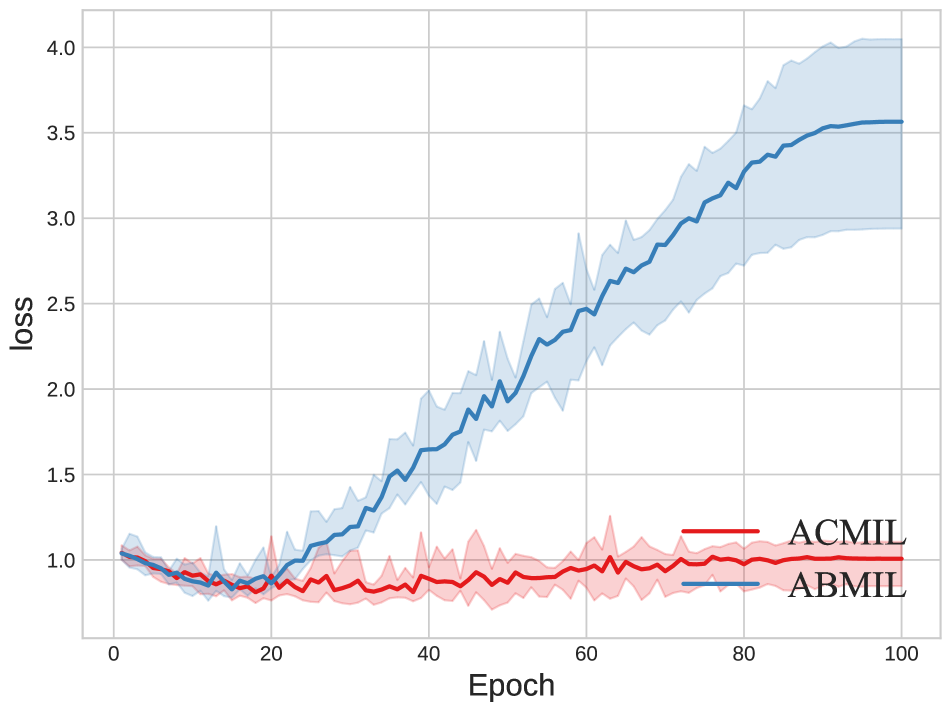
(a) Validation Loss

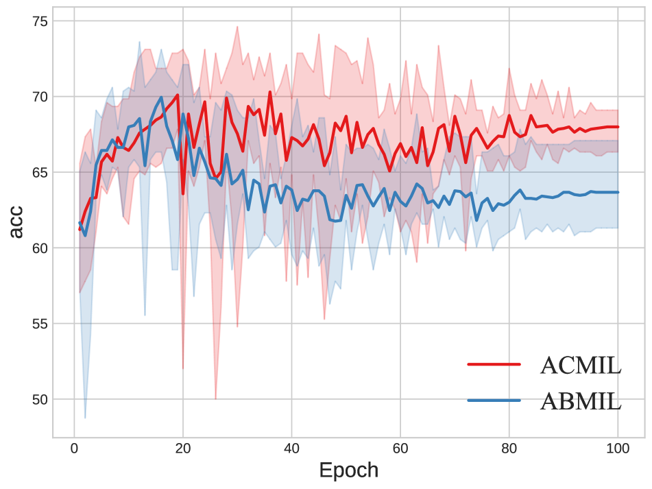
(b) Validation Accuracy

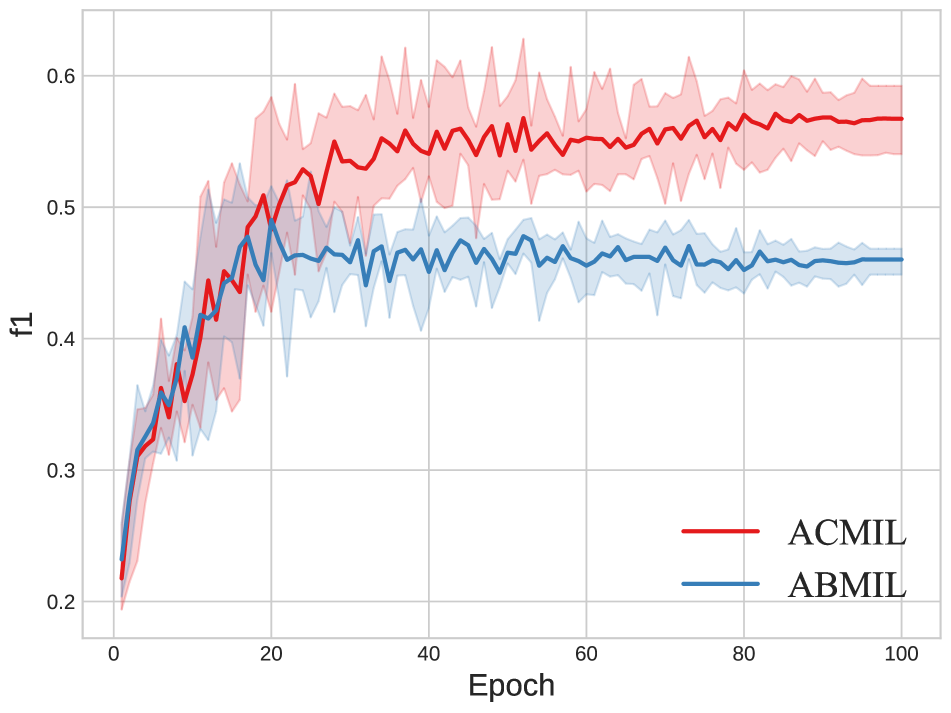
(c) Validation F1-score

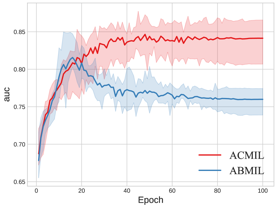
(d) Validation AUROC

Figure 1: Comparison of performance between ABMIL [27] and our ACMIL on the LBC validation set throughout the training process. ABMIL displays pronounced signs of overfitting, as indicated by a significant increase in validation loss and a decline in the other three evaluation metrics. Conversely, ACMIL effectively mitigates the overfitting issue.

Overfitting is a significant challenge in utilizing MIL methods for WSI analysis [60, 34, 47]. Common WSI datasets exhibit the intrinsic characteristics of limited data scale, ultra-high resolutions, and severe class imbalance, which makes overfitting more likely [2]. These datasets often consist of a relatively small number of slides, typically in the hundreds, each containing numerous patches, ranging from thousands to tens of thousands, with a relatively low proportion of positive cases. Moreover, pathology images are susceptible to data bias caused by variations in tissue preparations, staining protocols, and digital scanning methods [61, 34], which also is the key reason resulting in the overfitting [2]. As illustrated in Fig. 1, ABMIL [27], one of the most famous MIL methods, shows severe overfitting since loss drastically increases and validation metrics significantly decrease as the training processes.

Numerous efforts [25, 26, 36, 42, 49, 16, 45, 31, 47, 59, 34] have been made to mitigate the overfitting challenge and have been proven effective in improving evaluation metrics on standard benchmarks. Several of these works use attention heatmap as a valuable tool to analyze model interpretability. In fact, heatmap also plays a critical role in aggregating instance features into bag features, directly influencing the model’s ability against overfitting. Previous research rarely delves into the potential utility of heatmaps in analyzing the issue of overfitting.

Heatmap can clearly illustrate the overfitting challenge of attention mechanisms. Fig. 5 shows heatmaps of ABMIL predominantly concentrate on a subset of discriminative instances (i.e., the instances relevant to the bag label) while disregarding the remaining ones. However, recent studies [26, 49, 16] have shown that models trained solely on simple discriminative features could be susceptible to overfitting. In conclusion, the excessive concentration of attention values in the heatmap is closely linked to overfitting.

To mitigate the excessive concentration of attention values, we further analyze the heatmap of existing attention mechanism from two distinct perspectives. Firstly, there are various patterns among discriminative instances, and existing attention mechanisms tend to capture a part of them. To solve this, we introduce Multiple Branch Attention (MBA) method. MBA utilizes multiple attention branches, with each branch dedicated to capturing instances with distinct patterns, ensuring that more discriminative instances contribute to the final prediction. Secondly, in the existing attention mechanism, a small number of salient instances will occupy majority attention, resulting in overlooking sophisticated discriminative instances. To suppress these instances, we propose Stochastic Top-K Instance Masking (STKIM). STKIM randomly masks out a portion of instances with top-K attention values and then assigns their attention values to the remaining instances. Combining both of them, we propose the Attention-Challenging MIL (ACMIL) framework, aiming to force attention mechanisms to focus on more challenging instances.

We conduct experiments on three WSI datasets (i.e., Camelyon16, BRACS, and our in-house LBC dataset) with two backbones (i.e., ImageNet pre-trained ResNet18 and SSL pre-trained ViT/S-16). Experimental results demonstrate that our ACMIL significantly outperforms existing SOTA methods. We also present substantial experimental results, including heatmap visualization and UMAP visualization, to demonstrate the effectiveness of ACMIL in combatting overfitting.

2 Related Work

2.1 Combating Overfitting in WSI Analysis

In the domain of WSI analysis, combating the challenge of overfitting has received substantial attention. Next three paragraphs detail methods from three different aspects.

Some efforts have concentrated on enhancing the quality of instance representations. Early studies (e.g., [27, 6, 45]) rely on backbones pre-trained on the ImageNet dataset. However, the substantial domain gap between natural and pathological images hinder representation quality. Recent works (e.g., [48, 36, 15, 24, 53]) address this by emphasizing Self-Supervised Learning (SSL) to learn patch-level feature representations. In addition, efforts such as the work by Chen et al. [9] leverage hierarchical SSL for high-resolution image representations. Further, studies by Li et al. [31] and Wang et al. [52] demonstrate that fine-tuning the pre-trained encoder is essential for acquiring task-specific information.

Another line of research has explored correlation information between instances. For example, DSMIL [30] modeles correlation among multiscale instances. Furthermore, some studies introduce self-attention layers [45, 56, 43] and graph neural networks [21, 62, 8] to model correlations between different areas.

Further strategies have concentrated on data augmentation. Examples include DTFD-MIL [60], which introduces pseudo-bags for expanding bag counts and employed a double-tier MIL framework. IPS [4], Zoom-In Network [29], and Top-K MIL [12] generate bag representations by aggregating the representations of salient patches. Remix [57] and RankMix [11] introduce instance representation mixup for MIL. MHIM-MIL [47] augments bags by randomly masking salient instances.

While our STKIM shares similar motivation with MHIM-MIL [47], our approach is derived from heatmap analysis, whereas MHIM-MIL relies more on intuition. This distinction results in significant technical differences between the two solutions.

It’s noteworthy that our work is conducted independently and concurrently with MHIM-MIL.

2.2 Attention Heatmap for WSI analysis

Attention heatmap is valuable tool for assessing the interpretability of MIL methods [27]. Many existing methods [27, 15, 45, 30, 36, 55, 47, 59, 31] rely on heatmap visualizations to showcase their enhanced interpretability. It’s important to recognize that heatmaps play a central role in aggregating instance features into bag-level features, significantly impacting the model’s ability against the overfitting. This paper stands out by pioneering the use of heatmap as a tool for analyzing and addressing the overfitting challenge.

3 Method

Based on the ABMIL (detailed in Sec. 3.1), we present ACMIL to alleviate the overfitting problem, which is built on two components: Multiple Branch Attention (MBA) and Stochastic Top-K Instance Masking (STKIM). We describe the details of two components in Sec. 3.2 and 3.3, respectively.

3.1 ABMIL for WSI Analysis

In the binary MIL classification problem [6], a bag of instance, $\bm{X}=\{\bm{x}_{n}\}_{n=1}^{N}$, is associated with a single bag label, $\bm{Y}$. Each instance, $x_{n}$, is associated with a single binary label, $y_{n}$, which remains unknown during training. The assumption behind the MIL can be written as:

$$\bm{Y}=\begin{cases}0,&\text{ iff }\sum_{n=1}^{N}y_{n}=0\\ 1,&\text{ otherwise }\end{cases}$$ (1)

In the ABMIL [27], the multiple instance learning is modeled by a three-step process. i) Instance transformation into a low-dimensional embedding through neural networks: $\bm{h}_{n}=f(\bm{x}_{n})$. ii) Aggregation of all instance embeddings into the bag-level representation using an attention operator. Specifically, this operation is defined as:

$$\bm{z}=\sum_{n=1}^{N}a_{n}\bm{h}_{n},$$ (2)

Here, $a_{n}=\sigma(\bm{h}_{n})$ represents the attention values for $n$-th instance, $\bm{h}_{n}$. In the case of ABMIL, a gated attention (GA) mechanism [14] is adopted:

$$\sigma(\bm{h}_{n})=\frac{\exp\{\bm{w}^{\text{T}}(\text{tanh}(\bm{V}_{1}\bm{h}_{n})\odot\text{sigm}(\bm{V}_{2}\bm{h}_{n}))\}}{\sum_{j=1}^{N}\exp\{\bm{w}^{\text{T}}(\text{tanh}(\bm{V}_{1}\bm{h}_{j})\odot\text{sigm}(\bm{V}_{2}\bm{h}_{j}))\}},$$ (3)

where $\bm{V}_{1},\bm{V}_{2}\in\mathbb{R}^{L\times M}$, $\bm{w}\in\mathbb{R}^{L\times 1}$ are parameters, $\odot$ is an element-wise multiplication and $\mathrm{sigm(\cdot)}$ is the sigmoid non-linearity. iii) The bag prediction is generated based on the aggregated bag embedding: $\hat{\bm{Y}}=g(\bm{z})$.

3.2 Mutiple Branch Attention

Motivation. It is challenging to capture all discriminative instances using a single attention branch (see Fig. 2). This challenge arises due to variations in patterns among discriminative patches, stemming from differences in texture and morphology. Additionally, DNNs tend to exhibit a form of “laziness” where they prioritize capturing simpler patterns to minimize training loss, neglecting more intricate and challenging patterns [20, 19]. To tackle this issue, we design the MBA that captures more discriminative instances by multiple attention branches.

As depicted in Fig. 3 top view, the MBA firstly captures $M$ patterns and then aggregates their embeddings to make predictions. Each pattern is captured by an attention branch. To maintain both the discriminative nature of patterns and semantic diversity between them, we introduce two regularization techniques: semantic regularization and diversity regularization. Firstly, to ensure capturing discriminative patterns, the semantic regularization is accomplished by hanging a MLP layer behind each pattern embedding, equipping with the cross entropy loss function:

$$\mathcal{L}_{p}=-\frac{1}{M}\sum_{i=1}^{M}\bm{Y}\log{\bm{\hat{}}{\bm{Y}}_{i}}+\left(1-\bm{Y}\right)\log{\left(1-\bm{\hat{}}{\bm{Y}}_{i}\right)}$$ (4)

where $\bm{\hat{}}{\bm{Y}}_{i}=g_{i}(\bm{z}_{i})$ is the prediction based on $i$-th pattern embedding, $\bm{z}_{i}$. However, only equipping with cross-entropy loss may learn similar patterns and cannot dig out more discriminative information. To tackle this issue, we further introduce a diversity loss as follows:

$$\mathcal{L}_{d}=\frac{2}{M(M-1)}\sum_{i=1}^{M}\sum_{j=i+1}^{M}\cos(\bm{a}_{i},\bm{a}_{j})$$ (5)

where $\bm{a}_{i}$ consists of all attention values of $i$-th pattern, $\bm{a}_{i}=\{a_{i1},\cdots,a_{iN}\}$, also named heatmap as custom. The $\cos(\cdot)$ function is used to measure the similarity of the heatmaps between branches. By diversifying the heatmaps, the embedding of each branch can concentrate on different patterns.

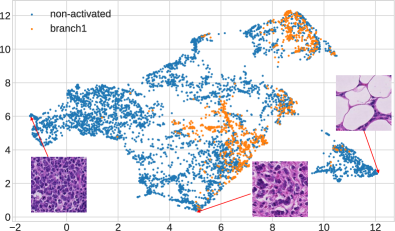
Figure 2: Motivation of MBA. UMAP visualization [39] of instance features in the tumor region of Camelyon16 ‘test_113’ case. There are various patterns/clusters among discriminative instances, and relying on one single branch tends to capture a part of clusters. Three instances are selected to exhibit their texture differences.

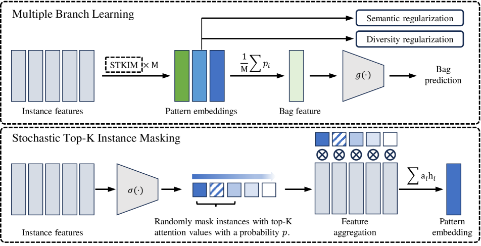
Figure 3: Overview of the proposed MBA (top view) and STKIM (bottom view). In the MBA, $M$ discriminative patterns are extracted from patch features using the attention operator regularized by semantic and diversity regularization terms. Then, a mean operator is performed to generate the bag feature, used for bag-level prediction. In the STKIM, $p\times 100\%$ instances with top-K attention values are masked randomly in the attention operator.

To aggregate the captured patterns to make predictions, the average of heatmaps is utilized as the heatmap of the whole bag:

$$\bm{a}=\frac{1}{M}\sum_{i=1}^{M}\bm{a}_{i}$$ (6)

where $\bm{a}$ is the heatmap of the whole bag, with a dimension of $N$. Then, the bag embedding can be obtained by aggregating the instance features using averaged heatmap $\bm{a}$. Moreover, since $\sum_{n=1}^{N}(\frac{1}{M}\sum_{i=1}^{M}a_{in})\bm{h}_{n}=\frac{1}{M}\sum_{i=1}^{M}(\sum_{n=1}^{N}a_{in}\bm{h}_{n})$, the bag embedding also can be formulated by applying mean pooling operator to pattern embeddings. The top view of Fig. 3 adopts the latter formulation for brevity. The loss function for the bag classifier is defined as:

$$\mathcal{L}_{b}=-\bm{Y}\log{\bm{\hat{}}{\bm{Y}}}+\left(1-\bm{Y}\right)\log{\left(1-\bm{\hat{}}{\bm{Y}}\right)}$$ (7)

Finally, the overall loss function for the ACMIL can be written as the combination of three loss terms defined in Eq. 4, 5 and 7,

$$\mathcal{L}=\mathcal{L}_{b}+\mathcal{L}_{p}+\mathcal{L}_{d}$$ (8)

Discussion. It’s important to highlight that when the parameter $M$ is set to 1 in MBA, it essentially mirrors the feature aggregation process of ABMIL, allowing for the discernment of a single pattern. In this sense, MBA serves as an extension of ABMIL, specifically designed to capture a more diverse set of patterns. We further discuss the connection between MBA and Multiple-Head Attention (MHA). HIPT [9] has unveiled that the distinct heads in MHA can effectively capture different visual concepts, akin to the role played by our MBA. However, these two techniques can be easily distinguished by: 1) MBA has the diversity regularization, ensuring that different branches can learn different concepts. This is absent in MHA. We demonstrate the critical role of $\mathcal{L}_{d}$ in Tab. 3. 2) MHA is a type of attention formulation, while MBA operates independently of the attention formulation, accommodating MHA within its framework. Appendix Tab. 4 reports the results of combining MHA and ACMIL.

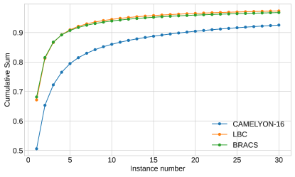
Figure 4: Motivation of STKIM. Accumulation of top-k attention values. Instances with top-k attention values occupy majority attention. Results are derived from features extracted through supervised pretraining.

3.3 Stochastic Top-K Instance Masking

Motivation. A small number of salient instances will occupy the majority attention in ABMIL while ignoring sophisticated discriminative instances. As depicted in Fig. 4, the sum of top-10 attention values is larger than 0.85 on all three datasets. However, the WSI typically involves more than 10 discriminative instances. For instance, in the Camelyon16 dataset, 129 out of 155 tumor slides contain 10 to 20,000 cancerous instances. In essence, numerous discriminative instances are overlooked. To deal with this issue, our proposed method, STKIM, aims to suppress the salient instances and assign more attention to remaining instances.

As depicted in Fig. 3 bottom view, STKIM introduces a masking operation into the attention mechanism, before feature aggregation and after attention values generation. The primary objective is to suppress top-k salient instances. A straightforward solution to achieve this is to mask out all of the top-k salient instances. However, this method poses certain challenges. It can result in the loss of information associated with key instances, which are crucial for discrimination. Furthermore, it might lead to a statistical mismatch between the feature representations before and after discarding these key instances. To address these issues, we draw inspiration from dropout [46] and cutout [16, 63] commonly used in computer vision. Our proposed solution employs stochastic masking for instance features with top-k attention values.

Specifically, we begin by sorting all attention values from highest to lowest. Subsequently, we randomly set the attention values of the top-k instances to 0, with a probability of $p$. This process can be formulated as:

$$a_{n}=\begin{cases}0,&\text{with probability }p\text{ and within top-K values}\\ a_{n},&\text{otherwise}\end{cases}$$ (9)

where $p$ and $K$ are two hyperparameters that control the intensity of masking. Following Eq. 9, we will assign the attention values of masked instances to the remaining instances by $a_{n}\rightarrow\frac{1}{\sum_{n=1}^{N}a_{n}}a_{n}$.

Discussion. While STKIM and MHIM-MIL [47] both adopt the technique that randomly masks instances with high attention values, there are notable technical distinctions between them. Firstly, MHIM-MIL adopts a two-stage training procedure where the model trained in the second stage is initialized using the best checkpoint obtained in the first stage. In contrast, STKIM is a one-stage framework that doesn’t require a pre-trained checkpoint beforehand, providing better scalability. Secondly, MHIM-MIL employs instance masking on a momentum teacher model, using the masked instances to train a student model. This involves two forward propagations for calculating attention values and producing bag predictions. On the other hand, STKIM utilizes a single model and necessitates only one forward propagation, resulting in faster execution compared to MHIM-MIL. Thirdly, MHIM-MIL incorporates three masking strategies and introduces five masking hyperparameters, which can be a complex and time-consuming trial-and-error process for reaching optimal performance. In contrast, STKIM primarily involves two hyperparameters, $p$ and $K$. Moreover, our ablation study in Appendix D.1 demonstrates that setting $p=0.6$ and $K=10$ achieves near-optimal performance across all datasets, significantly reducing the effort and time associated with trial-and-error tuning. Overall, STKIM has better scalability, faster execution, and reduced trial-and-error costs. In Appendix Sec. D.5, experimental results verify that our STKIM has faster execution, without compromising on performance.

Table 1: The performance of different MIL approaches across three datasets, two pre-trained methods, and two evaluation metrics. The most superior performance is highlighted in bold, while the second-best performance is indicated by underlining.

		CAMELYON-16		BRACS		LBC
		F1-score	AUC	F1-score	AUC	F1-score	AUC
ResNet-18 ImageNet pretrained	Max-pooling	0.582$\pm$0.170	0.620$\pm$0.155	0.489$\pm$0.047	0.738$\pm$0.014	0.476$\pm$0.033	0.775$\pm$0.010
	Mean-pooling	0.592$\pm$0.026	0.597$\pm$0.033	0.484$\pm$0.029	0.685$\pm$0.011	0.511$\pm$0.022	0.797$\pm$0.011
	Clam-SB	0.742$\pm$0.024	0.763$\pm$0.049	0.521$\pm$0.046	0.750$\pm$0.039	0.514$\pm$0.024	0.805$\pm$0.017
	TransMIL	0.643$\pm$0.088	0.706$\pm$0.076	0.444$\pm$0.040	0.732$\pm$0.043	0.385$\pm$0.013	0.693$\pm$0.027
	DSMIL	0.736$\pm$0.028	0.773$\pm$0.034	0.511$\pm$0.052	0.751$\pm$0.028	0.458$\pm$0.029	0.766$\pm$0.023
	DTFD-MIL	0.758$\pm$0.051	0.815$\pm$0.063	0.469$\pm$0.016	0.717$\pm$0.032	0.473$\pm$0.021	0.776$\pm$0.021
	IBMIL	0.777$\pm$0.009	0.799$\pm$0.050	0.510$\pm$0.043	0.726$\pm$0.034	0.489$\pm$0.017	0.791$\pm$0.021
	MHIM-MIL	0.752$\pm$0.034	0.772$\pm$0.026	0.511$\pm$0.022	0.774$\pm$0.021	0.543$\pm$0.037	0.816$\pm$0.009
	ABMIL	0.757$\pm$0.020	0.790$\pm$0.027	0.523$\pm$0.028	0.723$\pm$0.035	0.465$\pm$0.040	0.798$\pm$0.013
	ACMIL(ours)	0.798$\pm$0.029	0.841$\pm$0.030	0.552$\pm$0.048	0.754$\pm$0.008	0.546$\pm$0.028	0.821$\pm$0.015
ViT-S/16 SSL pretrained	Max-pooling	0.903$\pm$0.054	0.956$\pm$0.029	0.596$\pm$0.029	0.823$\pm$0.033	0.590$\pm$0.043	0.829$\pm$0.023
	Mean-pooling	0.577$\pm$0.057	0.569$\pm$0.081	0.522$\pm$0.038	0.739$\pm$0.007	0.559$\pm$0.024	0.827$\pm$0.012
	Clam-SB	0.925$\pm$0.035	0.969$\pm$0.024	0.631$\pm$0.034	0.863$\pm$0.005	0.617$\pm$0.022	0.865$\pm$0.018
	TransMIL	0.922$\pm$0.019	0.943$\pm$0.009	0.631$\pm$0.030	0.841$\pm$0.006	0.539$\pm$0.028	0.805$\pm$0.010
	DSMIL	0.943$\pm$0.007	0.966$\pm$0.009	0.577$\pm$0.028	0.816$\pm$0.028	0.562$\pm$0.028	0.820$\pm$0.033
	DTFD-MIL	0.948$\pm$0.007	0.980$\pm$0.011	0.612$\pm$0.080	0.870$\pm$0.022	0.612$\pm$0.034	0.842$\pm$0.010
	IBMIL	0.912$\pm$0.034	0.954$\pm$0.022	0.645$\pm$0.041	0.871$\pm$0.014	0.604$\pm$0.032	0.834$\pm$0.014
	MHIM-MIL	0.932$\pm$0.024	0.970$\pm$0.037	0.625$\pm$0.060	0.865$\pm$0.017	0.658$\pm$0.041	0.872$\pm$0.022
	ABMIL	0.914$\pm$0.031	0.945$\pm$0.027	0.680$\pm$0.051	0.866$\pm$0.029	0.595$\pm$0.036	0.831$\pm$0.022
	ACMIL(ours)	0.954$\pm$0.012	0.974$\pm$0.012	0.722$\pm$0.030	0.888$\pm$0.010	0.662$\pm$0.043	0.901$\pm$0.011

4 Experiments

4.1 Experimental Details

Datasets and Evaluation Metrics. The performance of ACMIL is evaluated on two public WSI datasets, i.e., Camelyon16 [3] and BRACS [5], and one private benchmark, LBC. Camelyon16 dataset consists of 400 WSIs in total, including 270 for training and 130 for testing. Following [60, 30], we further randomly split the training and validation sets from the official training set with a ratio of 9:1. We do not resplit BRACS dataset as it has been officially split to 395 of training set, 65 of validation set, and 87 of test set. We follow the challenge for a 3-class WSI classification: benign tumor, atypical tumor, and malignant. The liquid-based cytology (LBC) dataset collected 1,989 WSIs and included 4 classes, i.e., Negative, ASC-US, LSIL, and ASC-H/HSIL. We randomly split the whole dataset into training, validation, and test sets with the ratio of 6:2:2. Following [31], macro-AUC and macro-F1 scores are reported since all the three datasets are class imbalanced. Each of the main experiments is performed five times with random parameter initializations, and the average classification performance and standard deviation are reported. Besides, following [36, 60], the test performance is reported in epochs with the best validation performance.

Baselines. We systematically assess the efficacy of our ACMIL approach by benchmarking it against conventional MIL pooling strategies, Max-pooling and Mean-pooling, as well as contemporary attention-based techniques such as ABMIL [27], DSMIL [30], TransMIL [45], CLAM-SB [36], DTFD-MIL [60], MHIM-MIL [47], and IBMIL [34]. In pursuit of a comprehensive comparison across diverse aggregation operators, we utilize two distinct sets of features derived from ResNet-18 pre-trained on the ImageNet dataset [22] and ViT-S/16 pre trained using DINO [7] on a substantial collection of 36,666 WSIs [28]. The results of all other methods are reproduced using the official code they provide under the same settings.

Implementation Details. Implementation Details are placed in Appendix Sec. C.

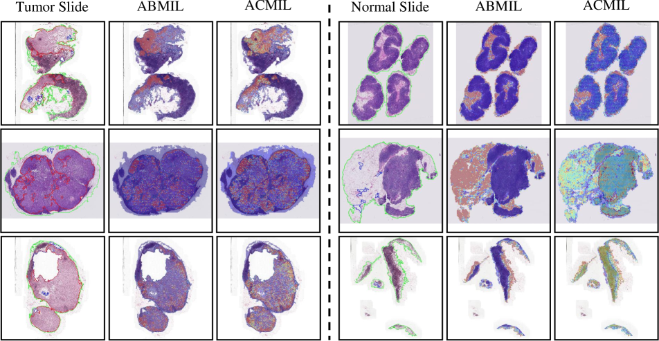
Figure 5: Heatmap visualization of WSI examples produced by ABMIL [27] (baseline) and our ACMIL. The left part shows three tumor WSIs that come from Camelyon16 dataset, and its tumor region is delineated by the red line. ACMIL generates attention values that cover a more extensive portion of the tumor region compared to ABMIL. The right part shows three normal WSIs that come from Camelyon16 dataset. ABMIL primarily focuses on a part of tissue such as adipose, while ACMIL extends its attention to the more normal tissues.

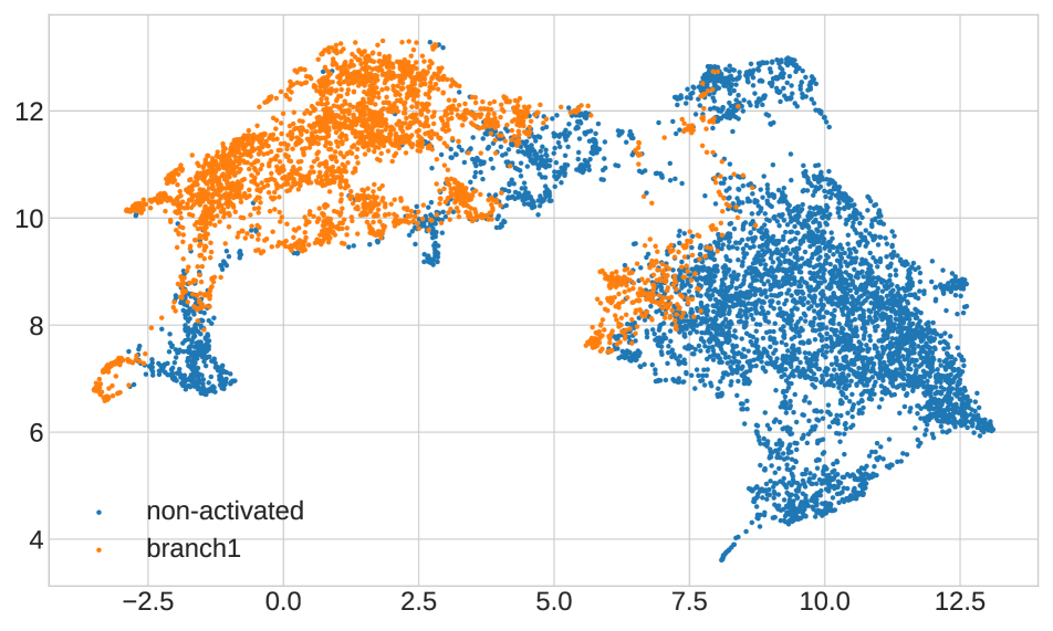
(a) ABMIL

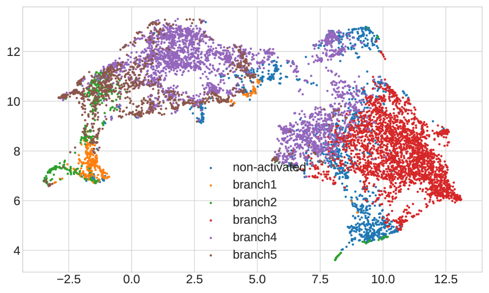
(b) ABMIL with MBA

Figure 6: UMAP visualization of instance features in the tumor region of the Camelyon16 ‘test_090’ case. The tumor instances display distinct patterns, posing a challenge for a single branch to capture all of them. As a result, ABMIL overlooks the right pattern/cluster. In contrast, The varying branch in MBA capture patterns separately, and combining them enable the activation of more patterns. An instance is considered active when its attention value surpasses $\frac{1}{N}$.

4.2 Performance Evaluation against SOTA

Tab. 1 provides a thorough comparison of performance between ACMIL and existing MIL methods. This evaluation spans three diverse datasets, involves two different choices for pretraining methods, and employs two crucial evaluation metrics, resulting in a comprehensive assessment with a total of 12 terms.

Considering the overall performance, ACMIL consistently outshines existing methods. It secures the top position in 10 out of the 12 metrics and holds the second position in the remaining 2 metrics. Specifically, for the Camelyon16, ACMIL achieves outstanding results using ResNet-18 pre-trained on ImageNet embeddings, surpassing the runner-up by 2.1% and 2.6% in terms of F1-score and AUC, respectively. On the other hand, with ViT-S/16 SSL pretrained embeddings, existing attention-based MIL methods exhibit remarkable performance, boasting F1-scores and AUC values exceeding 0.9. Notably, ACMIL achieves comparable performance with the former best-performing method, DTFD-MIL, in this setup.

For the BRACS, ACMIL demonstrates a substantial lead when utilizing ViT-S/16 SSL pre-trained embeddings, surpassing the second-best performance by margins of 4.2% and 1.7% in F1-score and AUC, respectively. Moreover, when employing ResNet-18 pre-trained on ImageNet embeddings, ACMIL achieves comparable performance with the previously top-performing method, MHIM-MIL. For the LBC, ACMIL stands out significantly among the other methods across all four metrics.

4.3 Heatmap Visualization

Fig. 5 presents heatmap visualizations illustrating examples of our approach’s performance in comparison to the baseline method, ABMIL [27]. Three tumor slides (left part) and three normal slides (right part) are selected to showcase the heatmap differences. Otherwise, due to the space limitation, we present more visualization in Appendix for further insights.

For the tumor slides, ABMIL tends to concentrate its attention on only a fraction of the tumor regions, potentially overlooking other significant areas. In contrast, ACMIL allocates attention across a wider spectrum of tumor regions, resulting in better alignment with expert annotations. For the normal slides, ABMIL predominantly focuses on specific tissue types, such as adipose tissue. This will lead to misinterpretation that only the adipose tissue is the normal tissue and other normal regions are uncorrelated to the WSI label. On the other hand, ACMIL effectively distributes attention values to encompass all normal regions, ensuring all regions are correlated for the WSI label. This approach closely mimics human intuition and satisfies the definition of the MIL formulation.

4.4 Further Analysis

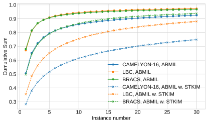
Figure 7: Comparison of accumulative sum of top-k attention values with STKIM and without STKIM. The use of STKIM helps alleviate the issue of excessive concentration of attention values within the top-K range..

MBA can capture diverse patterns. We employ UMAP [39] to visualize instance features within the tumor region of the Camelyon16 ‘test_090’ case. In Fig. 6(a), it’s evident that the tumor instances exhibit two primary patterns. However, ABMIL primarily activates the left pattern (colored orange) and neglects the right one. On the other hand, as demonstrated in Fig. 6(b), MBA’s various branches (branch1, branch2, branch3, and branch5) collectively capture the substructures of the left pattern, while branch4 specifically captures the right pattern. Combining all branches can capture more comprehensive patterns.

STKIM can suppress overly concentrated attention values. Fig. 7 illustrates a comparison of the cumulative sum of top-K attention values with and without STKIM. The plot clearly demonstrates that the use of STKIM helps mitigate the scenario where top-K attention values excessively dominate in the attention mechanism. This effect is particularly pronounced for the Camelyon16 dataset, where the cumulative sum of the top-10 values decreases from 0.87 to 0.6.

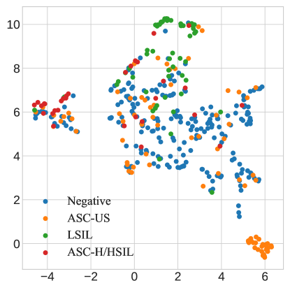
(a) ABMIL(V-measure=0.224)

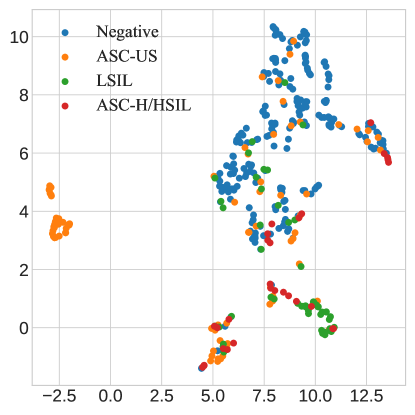
(b) ACMIL(V-measure=0.316)

Figure 8: UMAP visualization [39] of bag features for LBC test set. ACMIL learns more discriminative features than ABMIL effectively separating ‘LSIL’ and ‘ASC-H/HSIL’ features from the ‘Negative’ class. Improving feature separation is also corroborated by the V-measure score [44], a clustering metric that considers both the homogeneity and completeness of the clusters.

ACMIL can learn more discriminative bag features. We employ UMAP [39] to visualize bag features from the LBC test set, as illustrated in Fig. 8(a) and 8(b). This visualization demonstrates that our ACMIL is capable of learning more discriminative features compared to ABMIL. Specifically, it successfully separates the LSIL and ASC-H/HSIL clusters from the Negative cluster. To quantitatively assess this clustering performance, we employ the V-measure [44], following the methodology of Li et al. [31] and Diao et al. [17]. ACMIL achieves a V-measure score of 0.316, a significant improvement over ABMIL, which scores 0.224.

Table 2: Performance comparison between ACMIL with (w.) and without (w/o.) T-STKIM. The Gap column reports the performance difference between with and without T-STKIM. T-STKIM means using the STKIM at test phase. Using STKIM at test phase slightly reduces its performance.

ViT-S/16 SSL pre-trained Dataset Metric w. T-STKIM w/o. T-STKIM Gap(%) Camelyon F1-score 0.927$\pm$0.057 0.954$\pm$0.012 +2.7 AUC 0.967$\pm$0.017 0.974$\pm$0.012 +0.7 BRACS F1-score 0.697$\pm$0.033 0.722$\pm$0.030 +2.5 AUC 0.875$\pm$0.012 0.888$\pm$0.010 +1.3 LBC F1-score 0.637$\pm$0.034 0.662$\pm$0.043 +2.5 AUC 0.878$\pm$0.012 0.901$\pm$0.011 +2.3

ResNet-18 Imagenet pre-trained Dataset Metric w. T-STKIM w/o. T-STKIM Gap(%) Camelyon F1-score 0.780$\pm$0.026 0.798$\pm$0.029 +1.8 AUC 0.837$\pm$0.028 0.841$\pm$0.030 +0.4 BRACS F1-score 0.566$\pm$0.054 0.552$\pm$0.048 -1.4 AUC 0.750$\pm$0.021 0.754$\pm$0.008 +0.4 LBC F1-score 0.535$\pm$0.027 0.546$\pm$0.028 +1.1 AUC 0.808$\pm$0.019 0.821$\pm$0.015 +1.3

Table 3: Performance comparison between ACMIL with (w.) and without (w/o.) $\mathcal{L}_{d}$. The Gap column reports the performance difference between without and with $\mathcal{L}_{d}$. ACMIL without $\mathcal{L}_{d}$ drastically reduces its performance.

ViT-S/16 SSL pre trained Dataset Metric w/o. $\mathcal{L}_{d}$ w. $\mathcal{L}_{d}$ Gap(%) Camelyon F1-score 0.901$\pm$0.037 0.954$\pm$0.012 +5.3 AUC 0.943$\pm$0.027 0.974$\pm$0.012 +3.1 BRACS F1-score 0.642$\pm$0.046 0.722$\pm$0.030 +8.0 AUC 0.859$\pm$0.020 0.888$\pm$0.010 +2.9 LBC F1-score 0.603$\pm$0.023 0.662$\pm$0.043 +5.9 AUC 0.837$\pm$0.009 0.901$\pm$0.011 +6.4

ResNet-18 Imagenet pre-trained Dataset Metric w/o. $\mathcal{L}_{d}$ w. $\mathcal{L}_{d}$ Gap(%) Camelyon F1-score 0.747$\pm$0.022 0.798$\pm$0.029 +5.1 AUC 0.796$\pm$0.032 0.841$\pm$0.030 +5.5 BRACS F1-score 0.500$\pm$0.031 0.552$\pm$0.048 +5.2 AUC 0.760$\pm$0.026 0.754$\pm$0.008 -0.6 LBC F1-score 0.532$\pm$0.019 0.546$\pm$0.028 +1.4 AUC 0.809$\pm$0.018 0.821$\pm$0.015 +1.2

Do we need STKIM at the test phase? The answer is No. In Tab. 2, we present the outcomes of ACMIL with and without STKIM during the test phase, along with the performance differences between these settings. Across 11 out of 12 evaluation metrics, the version of ACMIL without STKIM during testing outperforms the version with STKIM slightly. This suggests that STKIM is not necessary during the test phase. Consequently, we can draw an analogy between the role of STKIM and masking data augmentation techniques such as cutout [16, 63].

Do we need diversity loss in MBA? The answer is Yes. In Tab. 3, we present the outcomes of ACMIL with and without $\mathcal{L}_{d}$, along with the performance differences between these settings. Notably, the last column clearly indicates a significant performance drop for ACMIL without $\mathcal{L}_{d}$. This emphasizes the crucial role of $\mathcal{L}_{d}$ in encouraging different branches to acquire distinctive discriminative knowledge within the MBA technique.

4.5 Ablation Study

Due to space limitation, we place the ablation study in Appendix Sec. D.1, with the main focus on the effect of hyperparameter $K,p,M$. Note that the effect of ablating MBA and STKIM is also discussed by setting $M=1$ and $K=0$, respectively.

5 Conclusion

Due to the intrinsic properties of WSI, MIL methods have often led to overfitting, limiting their applications. This paper reveal that the overly concentrated attention values in the heatmap is closely related to the overfitting. To address this, we propose the ACMIL approach, which is underpinned by two novel techniques: MBA and STKIM. Our experimental results on three datasets demonstrate ACMIL significantly surpasses SOTA methods. Moreover, this paper provides comprehensive experiments confirming the effectiveness of ACMIL in alleviating the overfitting problem. We hope our work can inspire future exploration into leveraging heatmaps for comprehensive analysis, encompassing both interpretability and generalization aspects. We also hope that our ACMIL can find valuable applications in a broader spectrum of WSI analysis tasks.

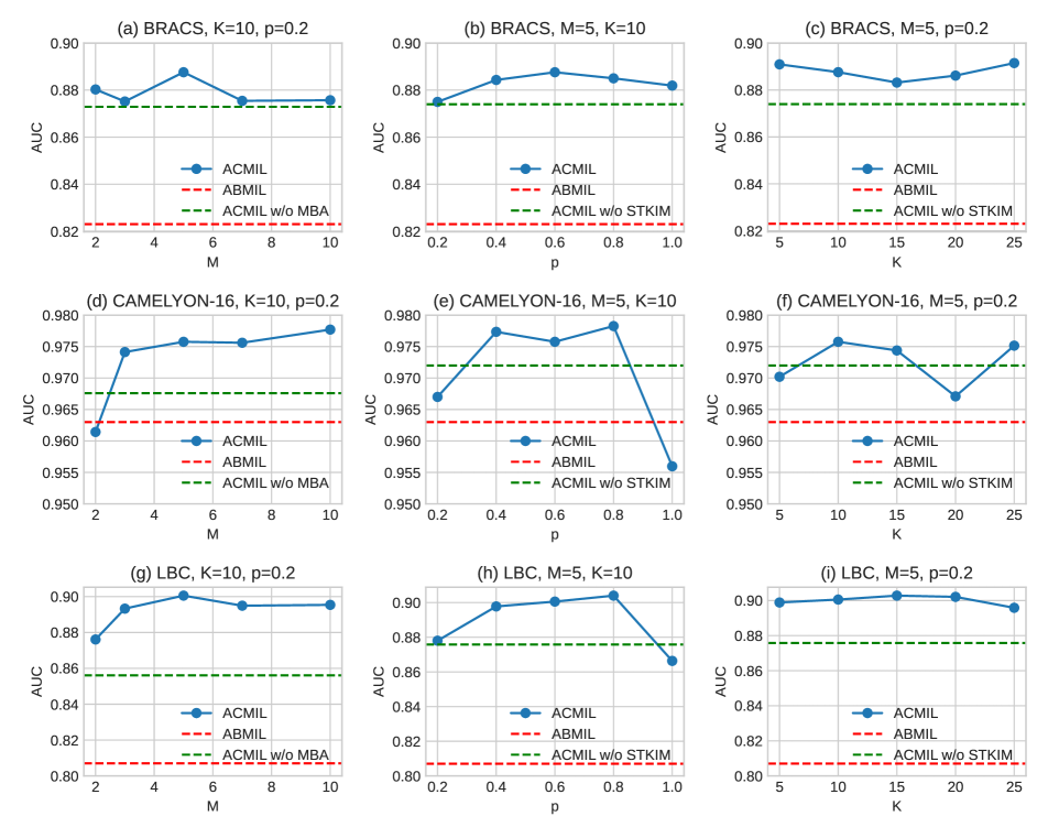
Figure 9: Hyperparameters sensitivity analysis on features extracted through the SSL pre-training. The effect of three hyperparameters, $K$, $p$, $M$, is investigated. Note that the red dot line denotes the performance of baseline, ABMIL, and the green dot line denotes the performance of ACMIL w/o MBA or STKIM. Five conclusions derived from the figure can be found in Sec. D.1.

Appendix A Overview

In the ACMIL appendix, we provide valuable resources and insights, including the source code (Sec. B), performance comparison against baseline, implementation details (Sec. C), additional experimental results (Sec. D), and a discussion on limitations (Sec. E).

Appendix B Source Code

The source code to train ACMIL is available at https://github.com/dazhangyu123/ACMIL. For further information on the environment setup and experiment execution, please refer to README.md. The implementation of ACMIL is based on the source code of ABMIL [27] and CLAM [36].

Appendix C Implementation Details

Data Pre-processing. We adopt the data pre-processing method from CLAM [36], which involves threshold segmentation and filtering to locate tissue regions in each whole-slide image (WSI). From these regions, we extract non-overlapping patches of size $256\times 256$ at a magnification of $\times 20$ for Camelyon16 and LBC datasets, and at a magnification of $\times 10$ for BRACS.

Feature Extraction. Given that ACMIL freezes the feature extractor during training, we extract and save features with 512 dimensions for ResNet-18 and 384 dimensions for ViT-S/16 to conserve space and expedite computation.

Model Architecture. The learnable components of the model include one fully-connected layer to reduce features to 256 dimensions for ResNet-18 and 128 dimensions for ViT-S/16, a gated attention network, and a fully-connected layer for making predictions.

Training. All models are trained for 100 epochs using a cosine learning rate decay starting at 0.0001 for ViT-S/16 and 0.0002 for ResNet-18. We employ an Adam optimizer with a weight decay of 0.0001, and the batch size is set to 1.

Hyperparameters. For the setting of Camelyon16 and natural supervised pre-training, we set hyperparameters as $M=2,K=10,p=0.6$. For the other situation, we set hyperparameters as $M=5,K=10,p=0.6$.

Appendix D More Experimental Results

The additional experimental results include ablation study (Sec. D.1), more heatmap visualizations (Sec. D.3), instance feature analysis for normal slides (Sec. D.4), and discussion for the computational cost of MBA (Sec. D.5).

Table 4: The performance comparison between the baseline and our ACMIL across two attention mechanisms (i.e., gated attention (GA) and multiple head attention (MHA)), three datasets, and two pretrained methods.

	CAMELYON-16		BRACS		LBC		Average
	F1-score	AUC	F1-score	AUC	F1-score	AUC
ResNet18 ImageNet pretrained
GA	0.757$\pm$0.020	0.790$\pm$0.027	0.523$\pm$0.028	0.723$\pm$0.035	0.465$\pm$0.040	0.798$\pm$0.013	0.676
+ACMIL	0.798$\pm$0.029	0.841$\pm$0.030	0.552$\pm$0.048	0.754$\pm$0.008	0.546$\pm$0.028	0.821$\pm$0.015	0.719
${\Delta}(\%)$	+4.1	+5.1	+2.9	+3.1	+8.1	+2.3	+4.3
MHA	0.752$\pm$0.030	0.775$\pm$0.027	0.502$\pm$0.039	0.738$\pm$0.019	0.531$\pm$0.025	0.817$\pm$0.011	0.686
+ACMIL	0.799$\pm$0.018	0.875$\pm$0.017	0.541$\pm$0.063	0.723$\pm$0.028	0.555$\pm$0.038	0.818$\pm$0.012	0.719
$\Delta(\%)$	+4.7	+10.0	+3.9	-1.5	+2.4	+0.1	+3.3
ViT-S/16 SSL pretrained
GA	0.914$\pm$0.031	0.945$\pm$0.027	0.680$\pm$0.051	0.866$\pm$0.029	0.595$\pm$0.036	0.831$\pm$0.022	0.805
+ACMIL	0.954$\pm$0.012	0.974$\pm$0.012	0.722$\pm$0.030	0.888$\pm$0.010	0.662$\pm$0.043	0.901$\pm$0.011	0.850
${\Delta}(\%)$	+4.0	+2.9	+4.2	+2.2	+6.7	+7.0	+4.5
MHA	0.931$\pm$0.032	0.961$\pm$0.017	0.656$\pm$0.030	0.850$\pm$0.030	0.619$\pm$0.032	0.864$\pm$0.013	0.813
+ACMIL	0.936$\pm$0.027	0.973$\pm$0.014	0.667$\pm$0.059	0.879$\pm$0.028	0.649$\pm$0.024	0.876$\pm$0.012	0.830
$\Delta(\%)$	+0.5	+1.2	+1.1	+2.9	+3.0	+1.2	+1.7

D.1 Ablation Study

Fig. 9 illustrates the AUC scores of ACMIL across three datasets when utilizing a ViT/B-16 feature extractor and varying hyperparameter settings. Several key observations emerge from these experiments:

Solely relying on MBA or STKIM can improving performance: Implementing either MBA or STKIM alone leads to significant performance improvements compared to ABMIL. The green dotted lines represent ACMIL’s AUC performance without MBA or STKIM, outperforming the red dotted lines (ABMIL’s performance) across all subfigures. Particularly noteworthy is the observation that MBA achieves better improvement than STKIM on all three datasets, with the green dot lines in the last two columns surpassing those in the first column, especially on the Camelyon and LBC datasets.

Combining MBA with STKIM further enhances performance beyond what can be achieved with either MBA or STKIM alone: Combining both MBA and STKIM yields performance improvements beyond what can be achieved with either MBA or STKIM individually. The blue dots represent ACMIL’s performance under different hyperparameter combinations, with 39 out of 45 blue dots exceeding the green horizontal lines.

Random Masking is important in STKIM: Random masking is a crucial aspect of STKIM. The second column demonstrates that setting $p=1.0$ leads to a performance deterioration across all three datasets. For LBC and Camelyon, a $p=1.0$ setting even results in performance lower than the green horizontal lines, indicating the ineffectiveness of STKIM without random masking.

Keeping $p=0.6$ or $p=0.8$ achieves better performance: The best performances across the three datasets are achieved at $p=0.6$ and $p=0.8$, as shown in the second column. Specifically, $p=0.6$ achieves the best performance on the BRACS dataset, whereas $p=0.8$ achieves the best performance on the other two datasets. In this paper, we set $p=0.6$ as the default value.

ACMIL is insensitive to the hyperparameter $K$: The hyperparameter $K$ exhibits minimal sensitivity, where different $K$ values result in a performance difference of less than 1.0% AUC. In practice, setting $K$ to 10 is generally sufficient for achieving near-optimal performance.

D.2 Performance Evaluation against Baseline

To assess the adaptability of our ACMIL to different attention mechanisms, we selected two prominent attention mechanisms as our baselines. The first is the gated attention (GA) mechanism [14], employed in approaches like ABMIL [27], CLAM [36], and DTFD-MIL [60]. The second is the multiple head attention (MHA) mechanism [50], utilized in methods such as TransMIL [45] and IPS transformer [4]. The results are presented in Table 4.

With GA as the baseline, ACMIL exhibits a substantial and comprehensive improvement in performance. All 12 performance metrics show enhancements, with an average gain of 4.4 points, a minimum increase of 2.2 points, and a maximum improvement of 8.1 points.

With MHA as the baseline, ACMIL also demonstrates performance improvements in the majority of terms (i.e., 11 out of 12 terms), achieving an average improvement of 2.5 points. In comparison to GA, MHA introduces parallel processing (i.e., heads). This modification enables the learning of different visual concepts across heads [9], contributing to a slight attenuation in the improvements brought by ACMIL.

D.3 More heatmap visualization

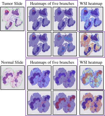
Figure 10: Heatmap visualizations for five attention branches. Different branches specialize in capturing specific features, contributing to the better interpretability for the bag (final) heatmap.

Heatmap visualizations of five attention branches in MBA. In Fig. 10, we present the heatmap visualizations for five attention branches and delve into the effects of these distinct branches. We’ve chosen two test slides in Camelyon16 for this analysis, including one tumor slide and one normal slide. For the tumor slide, we observe that all five branches capture the cancerous instances. Notably, the third and fifth branches successfully capture the entirety of the tumor regions, while the remaining three branches only manage to capture a subset of the tumor regions. Additionally, the third branch activates the adipose, and the fifth branch activates the lymphocytes regions. Overall, the averaged heatmap captures the whole tumor regions, along with slightly activating some normal regions. For the normal slide, the first two branches activate instances lying between adipose and lymphocytes regions. The third branch predominantly activates adipose tissue, the fourth branch emphasizes muscle regions, and the fifth branch highlights lymphocytes regions. Overall, the averaged heatmap activates all normal regions. This analysis illustrates how the different branches specialize in capturing specific features, contributing to a more comprehensive understanding of the data.

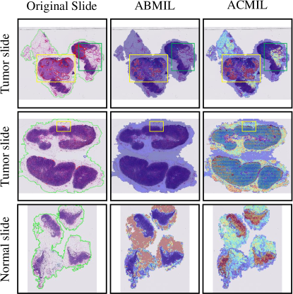
Figure 11: Heatmap visualizations with bad interpretability. Three cases indicates that ACMIL’s approach of assigning broader attention values to a wide range of predictive instances doesn’t consistently enhance interpretability.

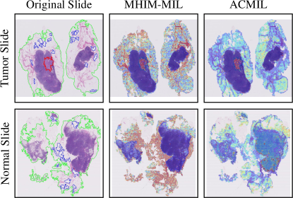
Figure 12: Comparison of heatmap visualizations between MHIM-MIL [47] and ACMIL (Zoom in for best view). ACMIL performs better on capturing comprehensive predictive instances.

Heatmap visualizations with bad interpretability. In Fig. 11, we present three cases (i.e., two tumor slides and one normal slide) with heatmap visualizations that exhibit poor interpretability. The first slide is a tumor slide. While ACMIL activates a greater number of cancerous instances than ABMIL (as indicated by the yellow box), it also activates some normal instances (visible in the green box). This mixed activation can potentially mislead experts during practical interpretability analysis. The second instance also concerns a tumor case but with small tumor regions. ABMIL accurately localizes the tumor regions (see yellow box). In contrast, ACMIL allocates more attention values to a broader range of predictive instances, which results in an inability to precisely locate the tumor regions. The third case pertains to a normal slide. In contrast to ABMIL, which provides misleading interpretability by predominantly focusing on adipose tissue, ACMIL assigns excessive attention values to lymphocytes regions. Consequently, the heatmap primarily highlights lymphocytes tissue instead of the expected comprehensive representation of normal tissue.

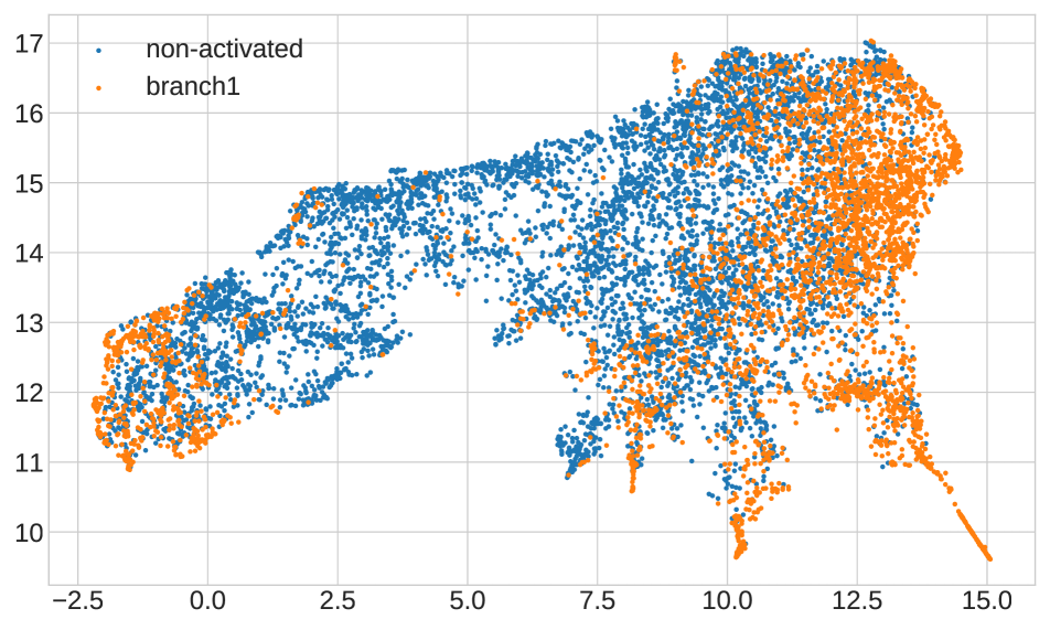
(a) ACMIL without MBA

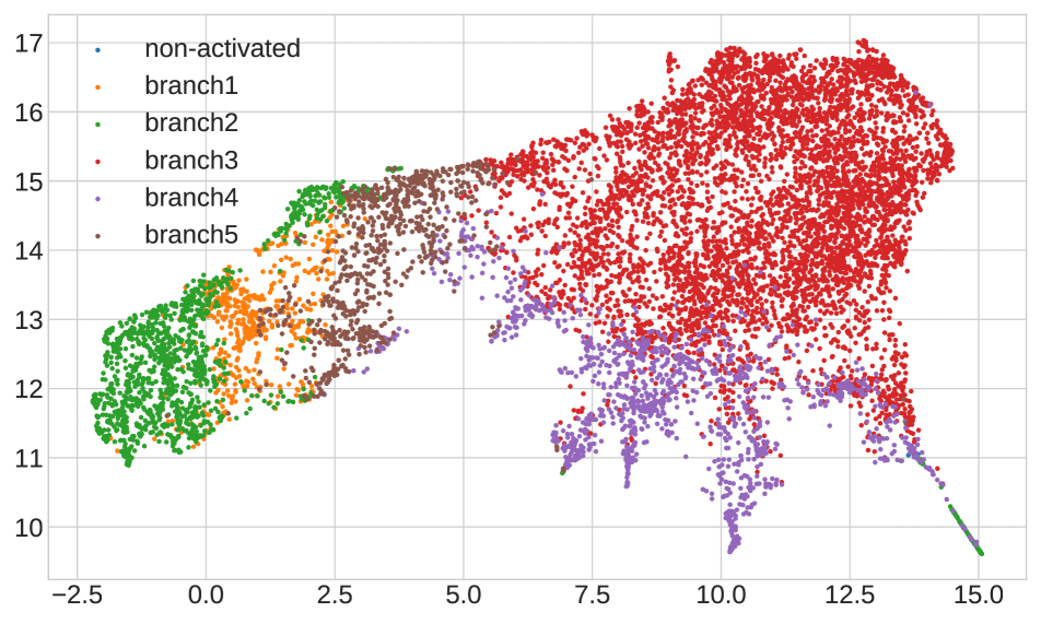
(b) ACMIL

Figure 13: UMAP visualization [39] of instance features in a normal case, Camelyon16 ’test_016’. The normal instances exhibit distinct patterns, making it challenging for a single-branch model like ABMIL to capture them comprehensively. Consequently, ABMIL may overlook certain instances. In contrast, our ACMIL leverages multiple branches, each adept at capturing specific patterns, enabling ACMIL to activate a greater number of normal instances. Note that the instance is considered active when its attention value surpasses $\frac{1}{N}$.

Comparison of heatmap visualization between MHIM-MIL [47] and ACMIL. In Fig. 12, we present the heatmap visualizations of MHIM-MIL and ACMIL. For the tumor slide (first row), MHIM-MIL and ACMIL both capture all cancerous instances in the tumor region, but MHIM-MIL activates more normal instances than ACMIL. For the normal slide (second row), MHIM-MIL predominately activates adipose, whereas ACMIL activate all normal instances more uniformly.

D.4 Instance feature analysis for normal slide

In Fig. 13, we present the UMAP visualization [39] of normal instance features in a typical Camelyon case, ’test_016’. The comparison between ABMIL and ACMIL is quite evident. ABMIL, with a single attention branch, activates only a fraction of normal instances. Conversely, ACMIL utilizes five branches, with each branch specializing in capturing specific patterns, resulting in the activation of nearly all normal instances. This observation demonstrates the superior ability of ACMIL to encompass a broader range of patterns in the data.

D.5 Discussion Combining Performance and Computational Cost

Table 5: Comparison of performance and computational cost requirements between MHIM-MIL and STKIM. We report the auc, FLOPs, training time per epoch (Time), and peak memory usage (Mem.) on the CAMELYON-16 (C16) dataset. The flops are measured with the number of instances of a bag being 1024.

Model	C16	BRACS	LBC	FLOPs	Time	Mem.
ResNet18 ImageNet pretrained
ABMIL	0.790	0.723	0.798	201M	8.0s	0.3G
MHIM-MIL	0.772	0.774	0.816	201M	20.8s	1.9G
STKIM	0.779	0.789	0.820	201M	8.0s	0.3G
ViT-S/16 SSL pretrained
ABMIL	0.945	0.866	0.831	84M	6.4s	0.2G
MHIM-MIL	0.970	0.865	0.872	84M	16.8s	1.0G
STKIM	0.968	0.873	0.856	84M	6.5s	0.2G

Table 6: Comparison of performance, time and memory requirements between ABMIL and MBA. We report the auc, the FLOPs, the training time per epoch (Time), and the peak memory usage (Mem.) on the CAMELYON-16 dataset (C16). The flops are measured with the number of instances of a bag being 1024.

Model	C16	BRACS	LBC	FLOPs	Time	Mem.
ResNet18 ImageNet pretrained
ABMIL	0.790	0.723	0.798	201M	8.0s	0.3G
+MBA	0.850	0.797	0.818	202M	11.6s	0.3G
ViT-S/16 SSL pretrained
ABMIL	0.945	0.866	0.831	84M	6.4s	0.2G
+MBA	0.973	0.878	0.875	85M	9.3s	0.2G

STKIM and MHIM-MIL [47]. We conducted a comprehensive comparison between STKIM and MHIM-MIL, focusing on computational cost and performance, as detailed in Tab. 5. For the computational cost, STKIM demonstrates nearly identical training time consumption and GPU memory usage as the baseline, ABMIL. This similarity arises because STKIM primarily integrates a sorting algorithm, which does not substantially increase resource requirements. On the other hand, MHIM-MIL introduces a teacher model while requiring two forward propagations, leading to significantly higher GPU memory usage and training time consumption. Due to the masking operator will be discarded in the evaluation, STKIM and MHIM-MIL keep the same evaluation cost (FLOPs) with the ABMIL. For the performance, STKIM delivers comparable results to MHIM-MIL across three datasets and with two pretrained backbone models. Notably, STKIM outperforms MHIM-MIL in four out of six performance metrics while lagging behind in the remaining two.

MBA. In Tab. 6, we present the comparison of performance and computational cost between ABMIL and MBA. Notably, MBA demonstrates a substantial performance improvement over ABMIL. Meanwhile, due to introducing a small number of parameters, the FLOPs and Memory cost increases marginally. Otherwise, the inclusion of the newly introduced diversity loss leads to a notable increase in time cost.

Appendix E Limitations

Even though our ACMIL is able to improve the model generalization ability and interprebility of MIL methods for WSI analysis, it still exist some limitations that are required to further explore in the future. Firstly, our ACMIL also will produce heatmap visualization with bad interpretability. Intuitively, this also will hurt the model generalization. To solve this, future work can further elaborate attention mechanism. Secondly, we find that the better representations will weaken the requirements for better attention design. Although we verify the effectiveness of our ACMIL on one of the currently best feature extraction methods, SSL pre-training, we still cannot ensure its scalability to the better representations.

References

- [1] Jaume Amores. Multiple instance classification: Review, taxonomy and comparative study. Artificial intelligence, 201:81–105, 2013.
- [2] Mohammad Mahdi Bejani and Mehdi Ghatee. A systematic review on overfitting control in shallow and deep neural networks. Artificial Intelligence Review, pages 1–48, 2021.
- [3] Babak Ehteshami Bejnordi, Mitko Veta, Paul Johannes Van Diest, Bram Van Ginneken, Nico Karssemeijer, Geert Litjens, Jeroen AWM Van Der Laak, Meyke Hermsen, Quirine F Manson, Maschenka Balkenhol, et al. Diagnostic assessment of deep learning algorithms for detection of lymph node metastases in women with breast cancer. Jama, 318(22):2199–2210, 2017.
- [4] Benjamin Bergner, Christoph Lippert, and Aravindh Mahendran. Iterative patch selection for high-resolution image recognition. arXiv preprint arXiv:2210.13007, 2022.
- [5] Nadia Brancati, Anna Maria Anniciello, Pushpak Pati, Daniel Riccio, Giosuè Scognamiglio, Guillaume Jaume, Giuseppe De Pietro, Maurizio Di Bonito, Antonio Foncubierta, Gerardo Botti, et al. Bracs: A dataset for breast carcinoma subtyping in h&e histology images. Database, 2022:baac093, 2022.
- [6] Gabriele Campanella, Matthew G Hanna, Luke Geneslaw, Allen Miraflor, Vitor Werneck Krauss Silva, Klaus J Busam, Edi Brogi, Victor E Reuter, David S Klimstra, and Thomas J Fuchs. Clinical-grade computational pathology using weakly supervised deep learning on whole slide images. Nature medicine, 25(8):1301–1309, 2019.
- [7] Mathilde Caron, Hugo Touvron, Ishan Misra, Hervé Jégou, Julien Mairal, Piotr Bojanowski, and Armand Joulin. Emerging properties in self-supervised vision transformers. In Proceedings of the IEEE/CVF international conference on computer vision, pages 9650–9660, 2021.
- [8] Tsai Hor Chan, Fernando Julio Cendra, Lan Ma, Guosheng Yin, and Lequan Yu. Histopathology whole slide image analysis with heterogeneous graph representation learning. In Proceedings of the IEEE/CVF Conference on Computer Vision and Pattern Recognition, pages 15661–15670, 2023.
- [9] Richard J Chen, Chengkuan Chen, Yicong Li, Tiffany Y Chen, Andrew D Trister, Rahul G Krishnan, and Faisal Mahmood. Scaling vision transformers to gigapixel images via hierarchical self-supervised learning. In Proceedings of the IEEE/CVF Conference on Computer Vision and Pattern Recognition, pages 16144–16155, 2022.
- [10] Richard J Chen, Ming Y Lu, Wei-Hung Weng, Tiffany Y Chen, Drew FK Williamson, Trevor Manz, Maha Shady, and Faisal Mahmood. Multimodal co-attention transformer for survival prediction in gigapixel whole slide images. In Proceedings of the IEEE/CVF International Conference on Computer Vision, pages 4015–4025, 2021.
- [11] Yuan-Chih Chen and Chun-Shien Lu. Rankmix: Data augmentation for weakly supervised learning of classifying whole slide images with diverse sizes and imbalanced categories. In Proceedings of the IEEE/CVF Conference on Computer Vision and Pattern Recognition, pages 23936–23945, 2023.
- [12] Philip Chikontwe, Meejeong Kim, Soo Jeong Nam, Heounjeong Go, and Sang Hyun Park. Multiple instance learning with center embeddings for histopathology classification. In Medical Image Computing and Computer Assisted Intervention–MICCAI 2020: 23rd International Conference, Lima, Peru, October 4–8, 2020, Proceedings, Part V 23, pages 519–528. Springer, 2020.
- [13] Toby C Cornish, Ryan E Swapp, and Keith J Kaplan. Whole-slide imaging: routine pathologic diagnosis. Advances in anatomic pathology, 19(3):152–159, 2012.
- [14] Yann N Dauphin, Angela Fan, Michael Auli, and David Grangier. Language modeling with gated convolutional networks. In International conference on machine learning, pages 933–941. PMLR, 2017.
- [15] Olivier Dehaene, Axel Camara, Olivier Moindrot, Axel de Lavergne, and Pierre Courtiol. Self-supervision closes the gap between weak and strong supervision in histology. arXiv preprint arXiv:2012.03583, 2020.
- [16] Terrance DeVries and Graham W Taylor. Improved regularization of convolutional neural networks with cutout. arXiv preprint arXiv:1708.04552, 2017.
- [17] James A Diao, Jason K Wang, Wan Fung Chui, Victoria Mountain, Sai Chowdary Gullapally, Ramprakash Srinivasan, Richard N Mitchell, Benjamin Glass, Sara Hoffman, Sudha K Rao, et al. Human-interpretable image features derived from densely mapped cancer pathology slides predict diverse molecular phenotypes. Nature communications, 12(1):1613, 2021.
- [18] Thomas G Dietterich, Richard H Lathrop, and Tomás Lozano-Pérez. Solving the multiple instance problem with axis-parallel rectangles. Artificial intelligence, 89(1-2):31–71, 1997.
- [19] Robert Geirhos, Jörn-Henrik Jacobsen, Claudio Michaelis, Richard Zemel, Wieland Brendel, Matthias Bethge, and Felix A Wichmann. Shortcut learning in deep neural networks. Nature Machine Intelligence, 2(11):665–673, 2020.
- [20] Robert Geirhos, Patricia Rubisch, Claudio Michaelis, Matthias Bethge, Felix A Wichmann, and Wieland Brendel. Imagenet-trained cnns are biased towards texture; increasing shape bias improves accuracy and robustness. arXiv preprint arXiv:1811.12231, 2018.
- [21] Yonghang Guan, Jun Zhang, Kuan Tian, Sen Yang, Pei Dong, Jinxi Xiang, Wei Yang, Junzhou Huang, Yuyao Zhang, and Xiao Han. Node-aligned graph convolutional network for whole-slide image representation and classification. In Proceedings of the IEEE/CVF Conference on Computer Vision and Pattern Recognition, pages 18813–18823, 2022.
- [22] Kaiming He, Xiangyu Zhang, Shaoqing Ren, and Jian Sun. Deep residual learning for image recognition. In Proceedings of the IEEE conference on computer vision and pattern recognition, pages 770–778, 2016.
- [23] Lei He, L Rodney Long, Sameer Antani, and George R Thoma. Histology image analysis for carcinoma detection and grading. Computer methods and programs in biomedicine, 107(3):538–556, 2012.
- [24] Simon Holdenried-Krafft, Peter Somers, Ivonne A Montes-Majarro, Diana Silimon, Cristina Tarín, Falko Fend, and Hendrik Lensch. Dual-query multiple instance learning for dynamic meta-embedding based tumor classification. arXiv preprint arXiv:2307.07482, 2023.
- [25] Le Hou, Dimitris Samaras, Tahsin M Kurc, Yi Gao, James E Davis, and Joel H Saltz. Patch-based convolutional neural network for whole slide tissue image classification. In Proceedings of the IEEE conference on computer vision and pattern recognition, pages 2424–2433, 2016.
- [26] Zeyi Huang, Haohan Wang, Eric P Xing, and Dong Huang. Self-challenging improves cross-domain generalization. In Computer Vision–ECCV 2020: 16th European Conference, Glasgow, UK, August 23–28, 2020, Proceedings, Part II 16, pages 124–140. Springer, 2020.
- [27] Maximilian Ilse, Jakub Tomczak, and Max Welling. Attention-based deep multiple instance learning. In International conference on machine learning, pages 2127–2136. PMLR, 2018.
- [28] Mingu Kang, Heon Song, Seonwook Park, Donggeun Yoo, and Sérgio Pereira. Benchmarking self-supervised learning on diverse pathology datasets. In Proceedings of the IEEE/CVF Conference on Computer Vision and Pattern Recognition, pages 3344–3354, 2023.
- [29] Fanjie Kong and Ricardo Henao. Efficient classification of very large images with tiny objects. In Proceedings of the IEEE/CVF Conference on Computer Vision and Pattern Recognition, pages 2384–2394, 2022.
- [30] Bin Li, Yin Li, and Kevin W Eliceiri. Dual-stream multiple instance learning network for whole slide image classification with self-supervised contrastive learning. In Proceedings of the IEEE/CVF conference on computer vision and pattern recognition, pages 14318–14328, 2021.
- [31] Honglin Li, Chenglu Zhu, Yunlong Zhang, Yuxuan Sun, Zhongyi Shui, Wenwei Kuang, Sunyi Zheng, and Lin Yang. Task-specific fine-tuning via variational information bottleneck for weakly-supervised pathology whole slide image classification. In Proceedings of the IEEE/CVF Conference on Computer Vision and Pattern Recognition, pages 7454–7463, 2023.
- [32] Ruoyu Li, Jiawen Yao, Xinliang Zhu, Yeqing Li, and Junzhou Huang. Graph cnn for survival analysis on whole slide pathological images. In International Conference on Medical Image Computing and Computer-Assisted Intervention, pages 174–182. Springer, 2018.
- [33] Yi Li and Wei Ping. Cancer metastasis detection with neural conditional random field. arXiv preprint arXiv:1806.07064, 2018.
- [34] Tiancheng Lin, Zhimiao Yu, Hongyu Hu, Yi Xu, and Chang-Wen Chen. Interventional bag multi-instance learning on whole-slide pathological images. In Proceedings of the IEEE/CVF Conference on Computer Vision and Pattern Recognition, pages 19830–19839, 2023.
- [35] Geert Litjens, Clara I Sánchez, Nadya Timofeeva, Meyke Hermsen, Iris Nagtegaal, Iringo Kovacs, Christina Hulsbergen-Van De Kaa, Peter Bult, Bram Van Ginneken, and Jeroen Van Der Laak. Deep learning as a tool for increased accuracy and efficiency of histopathological diagnosis. Scientific reports, 6(1):26286, 2016.
- [36] Ming Y Lu, Drew FK Williamson, Tiffany Y Chen, Richard J Chen, Matteo Barbieri, and Faisal Mahmood. Data-efficient and weakly supervised computational pathology on whole-slide images. Nature biomedical engineering, 5(6):555–570, 2021.
- [37] Anant Madabhushi. Digital pathology image analysis: opportunities and challenges. Imaging in medicine, 1(1):7, 2009.
- [38] Oded Maron and Tomás Lozano-Pérez. A framework for multiple-instance learning. Advances in neural information processing systems, 10, 1997.
- [39] Leland McInnes, John Healy, and James Melville. Umap: Uniform manifold approximation and projection for dimension reduction. arXiv preprint arXiv:1802.03426, 2018.
- [40] Liron Pantanowitz, Paul N Valenstein, Andrew J Evans, Keith J Kaplan, John D Pfeifer, David C Wilbur, Laura C Collins, and Terence J Colgan. Review of the current state of whole slide imaging in pathology. Journal of pathology informatics, 2(1):36, 2011.
- [41] Hans Pinckaers, Bram Van Ginneken, and Geert Litjens. Streaming convolutional neural networks for end-to-end learning with multi-megapixel images. IEEE transactions on pattern analysis and machine intelligence, 44(3):1581–1590, 2020.
- [42] Linhao Qu, Manning Wang, Zhijian Song, et al. Bi-directional weakly supervised knowledge distillation for whole slide image classification. Advances in Neural Information Processing Systems, 35:15368–15381, 2022.
- [43] Linhao Qu, Zhiwei Yang, Minghong Duan, Yingfan Ma, Shuo Wang, Manning Wang, and Zhijian Song. Boosting whole slide image classification from the perspectives of distribution, correlation and magnification. In Proceedings of the IEEE/CVF International Conference on Computer Vision, pages 21463–21473, 2023.
- [44] Andrew Rosenberg and Julia Hirschberg. V-measure: A conditional entropy-based external cluster evaluation measure. In Proceedings of the 2007 joint conference on empirical methods in natural language processing and computational natural language learning (EMNLP-CoNLL), pages 410–420, 2007.
- [45] Zhuchen Shao, Hao Bian, Yang Chen, Yifeng Wang, Jian Zhang, Xiangyang Ji, et al. Transmil: Transformer based correlated multiple instance learning for whole slide image classification. Advances in neural information processing systems, 34:2136–2147, 2021.
- [46] Nitish Srivastava, Geoffrey Hinton, Alex Krizhevsky, Ilya Sutskever, and Ruslan Salakhutdinov. Dropout: a simple way to prevent neural networks from overfitting. The journal of machine learning research, 15(1):1929–1958, 2014.
- [47] Wenhao Tang, Sheng Huang, Xiaoxian Zhang, Fengtao Zhou, Yi Zhang, and Bo Liu. Multiple instance learning framework with masked hard instance mining for whole slide image classification. arXiv preprint arXiv:2307.15254, 2023.
- [48] David Tellez, Geert Litjens, Jeroen van der Laak, and Francesco Ciompi. Neural image compression for gigapixel histopathology image analysis. IEEE transactions on pattern analysis and machine intelligence, 43(2):567–578, 2019.
- [49] Rishabh Tiwari and Pradeep Shenoy. Overcoming simplicity bias in deep networks using a feature sieve. 2023.
- [50] Ashish Vaswani, Noam Shazeer, Niki Parmar, Jakob Uszkoreit, Llion Jones, Aidan N Gomez, Łukasz Kaiser, and Illia Polosukhin. Attention is all you need. Advances in neural information processing systems, 30, 2017.
- [51] Dayong Wang, Aditya Khosla, Rishab Gargeya, Humayun Irshad, and Andrew H Beck. Deep learning for identifying metastatic breast cancer. arXiv preprint arXiv:1606.05718, 2016.
- [52] Hongyi Wang, Luyang Luo, Fang Wang, Ruofeng Tong, Yen-Wei Chen, Hongjie Hu, Lanfen Lin, and Hao Chen. Iteratively coupled multiple instance learning from instance to bag classifier for whole slide image classification. arXiv preprint arXiv:2303.15749, 2023.
- [53] Xiyue Wang, Jinxi Xiang, Jun Zhang, Sen Yang, Zhongyi Yang, Ming-Hui Wang, Jing Zhang, Wei Yang, Junzhou Huang, and Xiao Han. Scl-wc: Cross-slide contrastive learning for weakly-supervised whole-slide image classification. Advances in neural information processing systems, 35:18009–18021, 2022.
- [54] Yinxi Wang, Kimmo Kartasalo, Philippe Weitz, Balazs Acs, Masi Valkonen, Christer Larsson, Pekka Ruusuvuori, Johan Hartman, and Mattias Rantalainen. Predicting molecular phenotypes from histopathology images: A transcriptome-wide expression–morphology analysis in breast cancer. Cancer research, 81(19):5115–5126, 2021.
- [55] Jinxi Xiang and Jun Zhang. Exploring low-rank property in multiple instance learning for whole slide image classification. In The Eleventh International Conference on Learning Representations, 2022.
- [56] Conghao Xiong, Hao Chen, Joseph Sung, and Irwin King. Diagnose like a pathologist: Transformer-enabled hierarchical attention-guided multiple instance learning for whole slide image classification. arXiv preprint arXiv:2301.08125, 2023.
- [57] Jiawei Yang, Hanbo Chen, Yu Zhao, Fan Yang, Yao Zhang, Lei He, and Jianhua Yao. Remix: A general and efficient framework for multiple instance learning based whole slide image classification. In International Conference on Medical Image Computing and Computer-Assisted Intervention, pages 35–45. Springer, 2022.
- [58] Jiawen Yao, Xinliang Zhu, Jitendra Jonnagaddala, Nicholas Hawkins, and Junzhou Huang. Whole slide images based cancer survival prediction using attention guided deep multiple instance learning networks. Medical Image Analysis, 65:101789, 2020.
- [59] Cui Yufei, Ziquan Liu, Xiangyu Liu, Xue Liu, Cong Wang, Tei-Wei Kuo, Chun Jason Xue, and Antoni B Chan. Bayes-mil: A new probabilistic perspective on attention-based multiple instance learning for whole slide images. In The Eleventh International Conference on Learning Representations, 2022.
- [60] Hongrun Zhang, Yanda Meng, Yitian Zhao, Yihong Qiao, Xiaoyun Yang, Sarah E Coupland, and Yalin Zheng. Dtfd-mil: Double-tier feature distillation multiple instance learning for histopathology whole slide image classification. In Proceedings of the IEEE/CVF Conference on Computer Vision and Pattern Recognition, pages 18802–18812, 2022.
- [61] Yunlong Zhang, Yuxuan Sun, Honglin Li, Sunyi Zheng, Chenglu Zhu, and Lin Yang. Benchmarking the robustness of deep neural networks to common corruptions in digital pathology. In International Conference on Medical Image Computing and Computer-Assisted Intervention, pages 242–252. Springer, 2022.
- [62] Yu Zhao, Fan Yang, Yuqi Fang, Hailing Liu, Niyun Zhou, Jun Zhang, Jiarui Sun, Sen Yang, Bjoern Menze, Xinjuan Fan, et al. Predicting lymph node metastasis using histopathological images based on multiple instance learning with deep graph convolution. In Proceedings of the IEEE/CVF Conference on Computer Vision and Pattern Recognition, pages 4837–4846, 2020.
- [63] Zhun Zhong, Liang Zheng, Guoliang Kang, Shaozi Li, and Yi Yang. Random erasing data augmentation. In Proceedings of the AAAI conference on artificial intelligence, volume 34, pages 13001–13008, 2020.
- [64] Xinliang Zhu, Jiawen Yao, Feiyun Zhu, and Junzhou Huang. Wsisa: Making survival prediction from whole slide histopathological images. In Proceedings of the IEEE conference on computer vision and pattern recognition, pages 7234–7242, 2017.