Translational symmetry broken magnetization plateau of the $S=1$ antiferromagnetic Heisenberg chain with competing anisotropies

Abstract

We investigate the $S=1$ antiferromagnetic quantum spin chain with the exchange and single-ion anisotropies in a magnetic field, using the numerical exact diagonalization of finite-size clusters, the level spectroscopy analysis, and the density matrix renormalization group (DMRG) methods. It is found that a translational symmetry broken magnetization plateau possibly appears at the half of the saturation magnetization, when the anisotropies compete with each other. The level spectroscopy analysis gives the phase diagram at half the saturation magnetization. The DMRG calculation presents the magnetization curves for some typical parameters and clarifies the spin structure in the plateau phase.

I Introduction

One-dimensional quantum spin systems have been attracting increasing attention both experimentally and theoretically in recent years.TLL There have been found various kinds of phenomena which was originated from the strong spin-spin interactions as well as the strong quantum fluctuations due to one dimension. Among these phenomena, the magnetization plateau is one of most interesting phenomena because it is a macroscopic quantized phenomenon with a topological background in many body spin systems. In the quantum spin chains, based on the Lieb-Schultz-Mattis theoremLSM , the rigorous necessary condition for the appearance of the plateau was derived as the formoshikawa

$$Q(S-\tilde{m})={\rm integer},$$ (1)

where $S$ and $\tilde{m}$ are the total spin and the magnetization per unit cell, and $Q$ is the periodicity of the ground state measured by the unit cell. The magnetization plateau for $Q\geq 2$ should be accompanied by the spontaneous translational symmetry breaking. The simple magnetization plateau for $Q=1$ has been theoretically predicted or experimentally observed in the following systems; the $S=3/2$ and $S=2$ anisotropic antiferromagnetic chainssakai1 ; kitazawa , the $S=1/2$ distorted diamond chainhonecker1 ; okamoto1 ; kikuchi ; gu-su ; honecker2 ; ananikian ; morita ; ueno ; filho , the $S=1/2$ trimerized chainhida ; okamoto-ssc ; oka-kita ; gong2 ; liu2 , the $S=1/2$ tetramerized chaingong ; mahdavifar ; jiang ; liu3 , the $S=1/2$ two-leg laddersugimoto3 ; sugimoto1 ; sugimoto2 ; sasaki ; rahaman , the $S=1/2$ three-leg spin ladder and tubecabra ; okamoto-tube ; li ; alecio ; farchakh , the $S=1/2$ and $S=1$ skewed systemsyin ; dey , the mixed spin chainyamamoto ; sakai2 ; tonegawa ; tenorio ; liu ; karlova ; yamaguchi , the $p$-leg laddercabra3 , the polymerized chaincabra2 ; chen etc.

For the $S=1$ chain case, when the unit cell is composed of one $S=1$ spin, the magnetization plateau at half of the saturation is impossible with $Q=1$ because Eq.(1) cannot be satisfied with $S=1$ and $\tilde{m}=1/2$. Thus the unit cell should be composed of two (more generally even number) $S=1$ spins (namely dimerization) for the realization of this half plateau. In this case the parameter set $S=2$ and $\tilde{m}=1$ satisfies Eq.(1) with $Q=1$. In fact, the half magnetization plateaus were experimentally observed in several $S=1$ chain materials with the dimerization narumi ; maximova . A phase diagram on the plane of the dimerization parameter versus the magnetization was numerically obtained by Yan et al.yan

The translational symmetry broken plateau for $Q\geq 2$ also has been revealed to appear in the following systems; the $S=1/2$ frustrated bond-alternating chaintotsuka , the $S=1/2$ zigzag chainokunishi1 ; okunishi2 ; metavitsiadis the $S=1$ frustrated chainnakano , the $S=1/2$ frustrated spin ladderokazaki1 ; okazaki2 ; nakasu ; sakai3 ; sugimoto3 ; sugimoto1 ; sugimoto2 ; sasaki , the $S=1$ frustrated spin ladderokamoto2 ; okamoto3 ; michaud ; kohshiro , etc. In most cases, the mechanism of the $Q\geq 2$ plateau has been based on the frustration. Recently the numerical diagonalization study on the $S=2$ antiferromagnetic chain indicated that the competing anisotropies possibly yields the $Q=2$ plateau at half the saturation magnetizationyamada , as well as the $Q=1$ plateau. Thus the competing anisotropies are expected to give rise to the $Q=2$ plateau, even without frustration.

However, the half magnetization plateau of $S=1$ chain without dimerization (namely, $Q=2$, $S=1$, $\tilde{m}=1/2$) has not been observed so farmaximova as far as we know, Thus we think that it is important to clarify the condition for the realization of the half plateau in the $S=1$ spin chains with $Q=2$, $S=1$, $\tilde{m}=1/2$.

Considering the above situation, in this paper we investigate the $S=1$ antiferromagnetic chain with the $XXZ$-coupling and single-ion anisotropies competing with each other, and clarify the condition for the $Q=2$ plateau at half the saturation magnetization. This may give the reason why such a plateau has not been experimentally observed, as well as provide a guide for finding or synthesizing the materials showing such a plateau. Using the numerical diagonalization of finite-size clusters and the level spectroscopy analysis, the phase diagram at half the saturation magnetization is presented. In addition the density matrix renormalization group (DMRG) calculation indicates that the $Q=2$ plateau actually appears on the magnetization curve. We also show the phase diagram of the magnetization process.

II Model

We investigate the magnetization process of the $S=1$ antiferromagnetic Heisenberg chain with the exchange and single-ion anisotropies, denoted by $\lambda$ and $D$, respectively. The Hamiltonian is given by

$${\cal H} ={\cal H}_{0}+{\cal H}_{Z},$$ (3)

$${\cal H}_{0} =\sum_{j=1}^{L}\left[S_{j}^{x}S_{j+1}^{x}+S_{j}^{y}S_{j+1}^{y}+\lambda S_{j}^{z}S_{j+1}^{z}\right]$$

$$+D\sum_{j=1}^{L}(S_{j}^{z})^{2},$$

$${\cal H}_{Z} =-H\sum_{j=1}^{L}S_{j}^{z}.$$ (4)

The exchange interaction constant is set to be unity as the unit of energy. For $L$-site systems, the lowest energy of ${\cal H}_{0}$ in the subspace where $\sum_{j}S_{j}^{z}=M$, is denoted as $E(L,M)$. The reduced magnetization $m$ is defined as $m=M/M_{\rm s}$, where $M_{\rm s}$ denotes the saturation of the magnetization, namely $M_{\rm s}=L$. $E(L,M)$ is calculated by the Lanczos algorithm under the periodic boundary condition ($\mbox{\boldmath$S$}_{L+1}=\mbox{\boldmath$S$}_{1}$). We consider the case when $\lambda$ is Ising-like and $D$ is $XY$-like, namely, $\lambda>1$ and $D>0$. Thus easy-axis $\lambda$ and easy-plane $D$ are competing with each other. If the magnetization plateau appears at $m=1/2$, the translational symmetry should be spontaneously broken and the two-fold degeneracy of the ground state should occur, namely $Q=2$.

III Phase diagram at $m=1/2$

In this section using the numerical diagonalization for finite-size clusters, the phenomenological renormalization group and the level spectroscopy analyses, we show that the magnetization plateau appears at $m=1/2$ for sufficiently large $\lambda$ and $D$, and present the phase diagram at $m=1/2$.

III.1 Phenomenological Renormalization Group

In order to confirm that the magnetization plateau really appears at $m=1/2$, we apply the phenomenological renormalization groupPRG for the plateau width $W$ defined as the form

$$W=E(L,M-1)+E(L,M+1)-2E(L,M),$$ (5)

where $M=L/2$. Since $W$ should be proportional to $1/L$ in the no-plateau case, the scaled width $LW$ would be independent of the system size $L$, while $W$ would increase with $L$ in the presence of plateau. Let us set $D=5.0$ as an example. With fixed $D=5.0$, $LW$ calculated for $L=$10, 12, 14 and 16 are plotted versus $\lambda$ in Fig. 1. It indicates that the plateau obviously appears for sufficiently large $\lambda$. However, it is difficult to determine the precise phase boundary with this method.

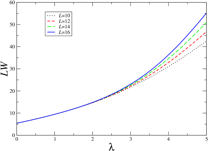
Figure 1: Scaled plateau width $LW$ plotted versus $\lambda$ for $L=$10, 12, 14 and 16 in the case of $D=5.0$.

Next, we apply the phenomenological renormalization group analysis PRG for the excitation gap with the momentum $k=\pi$ in the subspace $m=1/2$, defined as $\Delta_{\pi}$. The size-dependent fixed point $\lambda_{\rm c}(L+1)$ is determined by the equation

$$L\Delta_{\pi}(L,\lambda)=(L+2)\Delta_{\pi}(L+2,\lambda).$$ (6)

The scaled gaps $L\Delta_{\pi}$ for $D=5.0$ are plotted versus $\lambda$ for $L=$10, 12, 14 and 16 in Fig. 2. The size-dependent fixed points $\lambda_{\rm c}(L)$ for $L=$11, 13 and 15 are plotted versus $1/L$ for $D=5.0$ in Fig. 3. The phase boundary in the thermodynamic limit is estimated as $\lambda_{\rm c}=2.50\pm 0.01$. We repeat this procedure for various fixed $D$ or for fixed $\lambda$ to estimate the phase boundary. Actually, the phase boundary for $D\geq 3.0$ was obtained by fixed $D$ method, while that for $\lambda\geq 3.5$ estimated from the $\lambda$ method. The present result suggests that the translational symmetry is spontaneously broken and the ground state has a two-fold degeneracy in the plateau phase. The Néel order like $|\cdots 101010\cdots\rangle$ is expected to be realized. Thus we call this plateau ”Néel plateau”.

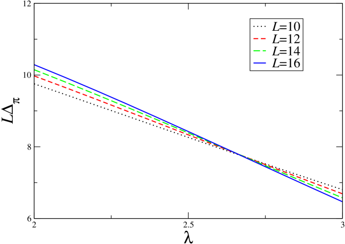
Figure 2: Scaled gap $L\Delta_{\pi}$ plotted versus $\lambda$ for $L=$10, 12, 14 and 16 in the case of $D=5.0$.

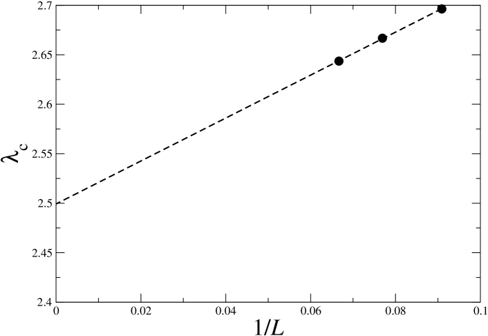
Figure 3: Size-dependent fixed points $\lambda_{\rm c}(L)$ obtained by the phenomenological renormalization group method for $L=$11, 13 and 15 are plotted versus $1/L$ for $D=5.0$. The phase boundary in the thermodynamic limit is estimated as $\lambda_{\rm c}=2.50\pm 0.01$.

III.2 Level spectroscopy

One of more precise methods to determine the phase boundary is the level spectroscopy analysis.oka-nom ; nom-oka Based on this method, comparing the single magnon excitation gap $\Delta_{1}\equiv W/2$ and $\Delta_{\pi}$, the gap $\Delta_{1}$ is smaller in the no-plateau phase, while $\Delta_{\pi}$ is smaller in the plateau phase. Thus $\Delta_{1}=\Delta_{\pi}$ gives the size-dependent phase boundary. $\Delta_{1}$ and $\Delta_{\pi}$ for $D=5.0$ are plotted versus $\lambda$ for $L=$12, 14 and 16 in Fig. 4. It indicates $L$ dependence is quite small and the size correction is predicted to be proportional to $1/L^{2}$. The extrapolation of $\lambda_{\rm c}$ to the thermodynamic limit gives $\lambda_{\rm c}=2.401\pm 0.001$, as shown in Fig. 5. Although there is a small discrepancy of the extrapolated phase boundary between the phenomenological renormalization and the level spectroscopy because of some finite-size effect, the latter method is expected to be more precise, because it is based on the essential nature of the Berezinskii-Kosterlitz-Thouless transition.berezinskii ; KT ; oka-nom ; nom-oka ; TLL ; jose Namely the lowest order contributions of the logarithmic size corrections are cancelled out with each other in the level spectroscopy method.oka-nom ; nom-oka

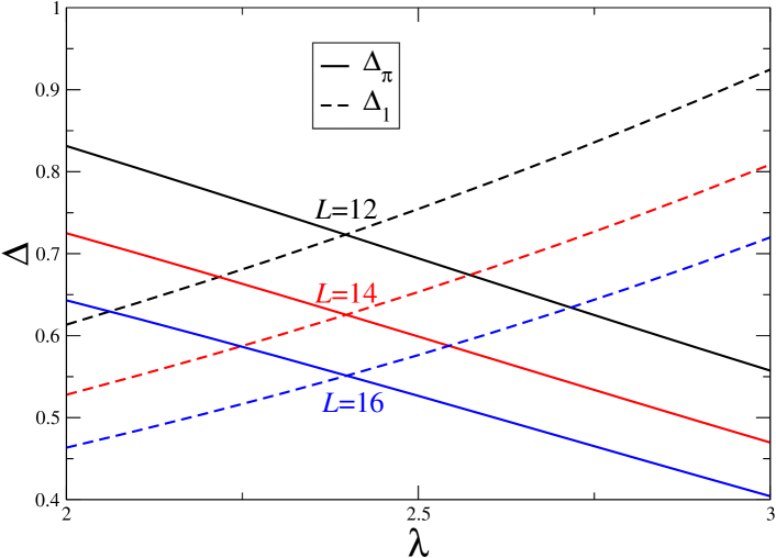
Figure 4: $\Delta_{1}$ and $\Delta_{\pi}$ for $D=5.0$ are plotted versus $\lambda$ for $L=$12, 14 and 16.

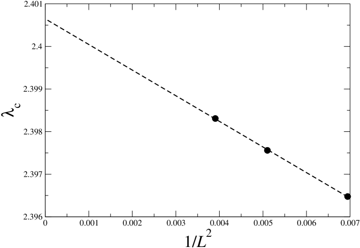
Figure 5: The extrapolation of $\lambda_{\rm c}$ to the thermodynamic limit, assuming the size correction if proportional to $1/L^{2}$, gives $\lambda_{\rm c}=2.401\pm 0.001$.

III.3 Magnetization jump

Apart from the no-plateau and the magnetization plateau phases, there is a parameter region where the $m=1/2$ magnetization is not realized due to the magnetization jump. like the spin flop transition. A typical case for the ”missing” can be seen in the magnetization curve of $\lambda=8.0$ and $D=0.0$ of Fig.8. There is a magnetization jump from about $m=0.04$ to $m=0.55$, which means that the $m=1/2$ situation is not realized in this curve. If the $m=1/2$ magnetization is included in the magnetization jump, we call that the system is in the missing region. The boundary of the missing region $D_{\rm m}$ for $\lambda=8.0$ is plotted versus $1/L$ in Fig. 6. Assuming the size correction proportional to $1/L$, $D_{\rm m}$ in the infinite length limit is estimated as $D_{\rm m}=1.64\pm 0.01$. The boundary of the missing region is determined by this method.

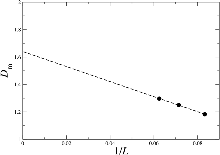
Figure 6: The boundary of the missing region $D_{\rm m}$ for $\lambda=8.0$ is plotted versus $1/L$. As assuming the size correction proportional to $1/L$, $D_{\rm m}$ in the infinite length limit is estimated as $D_{\rm m}=1.64\pm 0.01$.

III.4 Phase diagram

Here we present the phase diagram at half the saturation magnetization with respect to the easy-axis coupling anisotropy $\lambda$ and the easy-plane single-ion one $D$ in Fig. 7. It consists of the no-plateau, Néel plateau phases and the missing region which is surrounded by green triangles. In the Néel plateau phase the translational symmetry is spontaneously broken and $Q=2$ is realized.

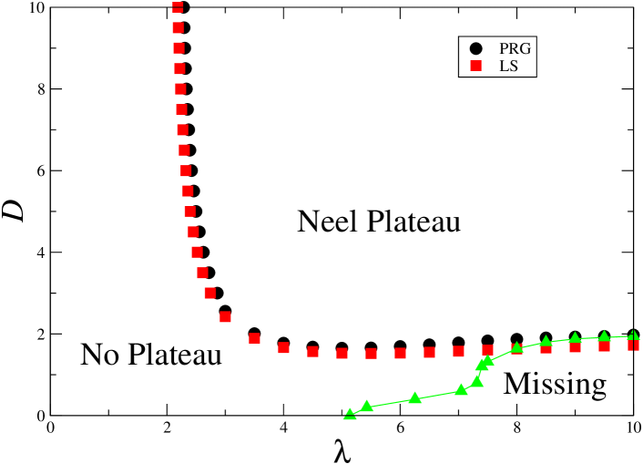
Figure 7: Phase diagram at $m=1/2$ of the present model. There are the no-plateau, Néel plateau phases and the missing region which is surrounded by green triangles.

IV Magnetization curves

In order to confirm that the 1/2 magnetization plateau actually appears, we performed the DMRG calculation with $L=100$ to obtain the magnetization curves in the ground state. The calculated magnetization curves for ($\lambda,D)=(4.0,4.0),~{}(5.0,3.0),~{}(6.0,2.0),~{}(7.0,1.0)$ and $(8.0,0.0)$ are shown in Fig. 8, by black circles, red squares, green pluses, blue crosses and brown stars, respectively. The curves for (5.0, 3.0) and (6.0, 2.0) in the plateau phase obviously exhibit the 1/2 magnetization plateau. On the curve for $(8.0,0.0)$ the $m=1/2$ state is skipped due to the magnetization jump. For the case of $(7.0,1.0)$ the $m=1/2$ state is realized, although there is a magnetization jump.

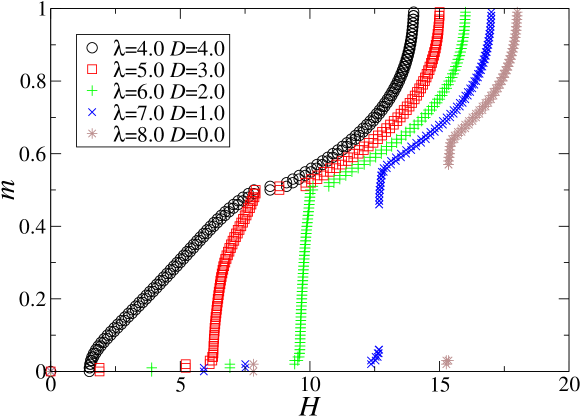
Figure 8: The magnetization curves calculated by DMRG for $(\lambda,D)=(4.0,4.0),~{}(5.0,3.0),~{}(6.0,2.0),~{}(7.0,1.0)$ and $(8.0,0.0)$ are shown by black circles, red squares, green pluses, blue crosses and brown stars, respectively.

The magnetization curves by DMRG for $(\lambda,D)=(4.0,4.0),~{}(3.0,5.0),~{}(2.0,6.0),~{}(1.0,7.0)$ and $(0.0,8.0)$ are also shown in Fig. 9, by black circles, red squares, green pluses, blue crosses and brown stars, respectively. The curves for (0.0, 8.0), (1.0, 7.0) and (2.0, 6.0) in the no-plateau phase have no plateau, while the ones for (3.0, 5.0) and (4.0, 4.0) in the plateau phase exhibit the $1/2$ plateau. These magnetization curves are all consistent with the phase diagram in Fig. 7.

The saturation field $H_{\rm s}$ can be calculated from the energy difference between the energy of the ferromagnetic state and that of the 1-spin-down state of the Hamiltonian (3). A simple calculation leads to

$$H_{\rm s}=2\lambda+D+2.$$ (7)

All the magnetization curves of Figs.8 and 9 were calculated under the condition $\lambda+D=8$, which leads to

$$H_{\rm s}=\lambda+10.$$ (8)

This well explains all of $H_{\rm s}$ in Figs. 8 and 9.

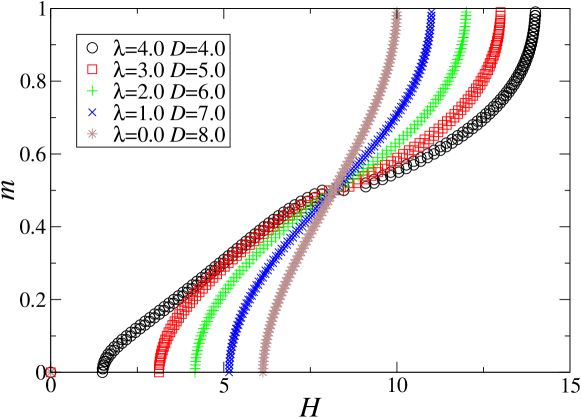
Figure 9: The magnetization curves calculated by DMRG for $(\lambda,D)=(4.0,4.0),~{}(3.0,5.0),~{}(2.0,6.0),~{}(1.0,7.0)$ and $(0.0,8.0)$ are shown by by black circles, red squares, green pluses, blue crosses and brown stars, respectively.

V Spin structure

In order to investigate the spin structure at the 1/2 magnetization plateau, we calculated the magnetization at each site by DMRG. The site magnetization $\langle S_{j}^{z}\rangle$ at $m=1/2$ for ($\lambda,D)=(4.0,4.0)$ in the plateau phase is shown in Fig. 10. It indicates that the translational symmetry is spontaneously broken and the periodicity $Q=2$ is realized. It is consistent with the physical picture of the Néel plateau.

Figure 10: Site magnetization $\langle S_{j}^{z}\rangle$ for $(\lambda,D)=(4.0,4.0)$ in the Néel plateau phase by DMRG with $L=100$. We can see the Néel-type structure $|\cdots 101010\cdots\rangle$.

VI Effective Theory

Let us start with the isolated spin limit to construct an effective theory. For the case of $m=1/2$, the $|S^{z}=0\rangle$ state and the $|S^{z}=1\rangle$ state have the same energies, which are lower than the energy of the $|S^{z}=-1\rangle$ state by $2D$. We can construct an effective theory by picking up only the $|S^{z}=0\rangle$ state and the $|S^{z}=1\rangle$ state when $D$ is sufficiently larger than the interactions, namely

$$D\gg\lambda.$$ (9)

We introduce the pseudo-spin operator $T$ with $T=1/2$, where $|T^{z}=1/2\rangle$ and $|T^{z}=-1/2\rangle$ represent $|S^{z}=1\rangle$ and $|S^{z}=0\rangle$, respectively. In this restricted basis, we see

$$S^{z}=T^{z}+{1\over 2},~{}~{}~{}~{}S^{\pm}=\sqrt{2}T^{\pm}.$$ (10)

Therefore we obtain the effective Hamiltonian as

$${\cal H}_{\rm eff} = \sum_{j=1}^{L}\left\{2(T_{j}^{x}T_{j+1}^{x}+T_{j}^{y}T_{j+1}^{y})+\lambda T_{j}^{z}T_{j+1}^{z}\right\}$$ (11)

$$+(\lambda+D-H)\sum_{j=1}^{L}T_{j}^{z}+L{\lambda+D+H\over 4}.$$

The condition $\sum_{j}T_{j}^{z}=0$ corresponds to $m=1/2$ of the original model. From the exact solution,TLL the ground-state of ${\cal H}{\rm eff}$ for $\sum_{j}T_{j}^{z}=0$ is either the Tomonaga-Luttinger liquid stateTLL (no plateau of the original model) or the Néel state (plateau with the Néel mechanism of the original model) according as $\lambda\leq 2$ or $\lambda>2$. We note that there is a factor 2 in front of $T_{j}^{x}T_{j+1}^{x}+T_{j}^{y}T_{j+1}^{y}$ in Eq.(11). Thus the behavior of the boundary between the plateau and no plateau phase $\lambda\to 2$ as $D\to\infty$ in Fig. 7 is well explained. The magnetic field $H_{1/2}$ corresponding to $m=1/2$ can be obtained from the condition that the effective field for the $T$-system is zero, namely $\lambda+D-H_{1/2}=0$, resulting in

$$H_{1/2}=\lambda+D.$$ (12)

For the magnetization curves of Figs. 8 and 9, we set $\lambda+D=8$. Then DMRG results $H_{1/2}\simeq 8$ for all the curves of Fig. 9 are also well explained by this effective theory. For the magnetization curves in Fig. 8, this effective theory does not hold because Eq.(9) is not satisfied.

In the phase diagram Fig.7, we see that two features in the $\lambda\to\infty$ limit. One is that (a) the plateau-no plateau line and the missing boundary line are going to merge, and the other is that (b) the critical value of $D$ tends to $D_{\rm c}\simeq 2$. Liu et al.liu-ssc investigated the phase diagram of the $S=1$ Ising chain

$${\cal H}=\sum_{j=1}^{L}S_{j}^{z}S_{j+1}^{z}+D_{0}\sum_{j=1}^{L}(S_{j}^{z})^{2}-H\sum_{j=1}^{L}S_{j}^{z}.$$ (13)

to obtain the phase diagram on the $D_{0}-H$ plane. The feature (a) is consistent with the phase diagram of Liu et al., although the feature (b) cannot be explained by it since the transverse coupling is not included their Hamiltonian (13).

VII Phase diagram of magnetization process

In order to consider some realistic experiments, it would be useful to obtain the phase diagram of the magnetization process summarizing the spin structure. In the gapless phase of the magnetization process, the system is expected to be in the Tomonaga-Luttinger liquid phase. It is characterized by the power-law decay of the spin correlation functions which have the asymptotic forms

$$\langle S_{0}^{z}S_{r}^{z}\rangle-m^{2}\sim\cos(2k_{\rm F}r)r^{-{\eta}_{z}},$$ (14)

$$\langle S_{0}^{x}S_{r}^{x}\rangle\sim(-1)^{r}r^{-\eta_{x}}$$ (15)

in the infinite $r$ limit. $2k_{\rm F}$ is $\pi(1-m)$ in the present model. The first equation corresponds to the SDW spin correlation parallel to the external field and the second one corresponds to the Née-like spin correlation perpendicular to the external field. The smaller exponent between $\eta_{z}$ and $\eta_{x}$ determines the dominant spin correlation. In the conventional magnetization process the canted Néel-like spin correlation is dominant, namely $\eta_{x}<\eta_{z}$. However, in some frustrated systems the magnetization region where $\eta_{z}<\eta_{x}$ is realized appears and the incommensurate spin correlation parallel to the external field is dominant there.maeshima Then we consider the possibility of a similar interesting behavior in the present model. According to the conformal field theory these exponents can be estimated by the formscardy

$$\eta_{x}={{E(L,M+1)+E(L,M-1)-2E(L,M)}\over{E_{k_{1}}(L,M)-E(L,M)}},$$ (16)

$$\eta_{z}=2{{E_{2k_{F}}(L,M)-E(L,M)}\over{E_{k_{1}}(L,M)-E(L,M)}},$$ (17)

for each magnetization $M$, where $k_{1}$ is defined as $k_{1}=L/2\pi$. Since the relation $\eta_{x}\eta_{z}=1$ is satisfied in the Tomonaga-Luttinger liquid phase, we have only to calculate one of these two exponents to determine the dominant spin correlation. We estimate the exponent $\eta_{x}$ here, because the calculation of $\eta_{z}$ meets the larger finite-size correlation due to the incommensurate correlation expressed by the cosine factor in Eq. (15). The estimated exponent $\eta_{x}$ by the numerical exact diagonalization for $L=16$ and $\lambda=4.0$ is plotted versus the magnetization $m$ for several values of $D$ in Fig. 11. In the case of $D\geq 3.0$, the magnetization region where $\eta_{x}$ is larger than 1 appears around $m\sim 1/2$. It indicates that the $z$ component dominant Tomonaga-Luttinger liquid phase takes place. Using the numerical exact diagonalization for $L=16$, $\eta_{x}$ can be calculated for $M=1,2,\cdots,15$. Then we estimate the crossover line $\eta_{x}=1$, interpolating linearly the calculated values of $\eta_{x}$ at $M$ and $M+1$ between which $\eta_{x}=1$ would occur. In addition we estimate the critical point $D_{c}$ where the magnetization jump begins at each $M$ using the numerical exact diagonalization for $L=16$. The estimated crossover line between the $z$ component dominant Tomonaga-Luttinger liquid ($z$TLL) phase and the $xy$ component dominant one ($xy$TLL), and the critical line of the magnetization jump are shown in the $D$ and magnetization phase diagram for $\lambda=4.0$ in Fig. 12. In order to confirm whether the crossover line really exists even in the thermodynamic limit, we also calculate $\langle S_{j}^{x}S_{j+r}^{x}\rangle$ for the central region of an $L=100$ chain with DMRG, and then estimate the exponent of its power-law decay for $r=1\sim 30$. These crossover lines estimated by the numerical exact diagonalization and by the DMRG are shown as blue crosses and blue circles, respectively in Fig. 12. They are consistent with each other and it suggests that the $z$TLL phase is realized even in the infinite length limit. In conclusion, it is found that the present competing anisotropies give rise to the 1/2 translational symmetry broken magnetization plateau and the incommensurate parallel spin correlation dominant Tomonaga-Luttinger liquid ($z$TLL) phase around the plateau. Even for different $\lambda$, qualitatively similar phase diagrams would be obtained.

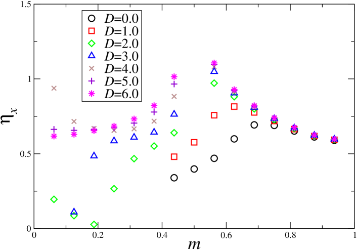
Figure 11: Exponent $\eta_{x}$ estimated by the numerical exact diagonalization of the 16-spin system for $\lambda=4.0$ plotted versus $m$ for $D=$0.0 (black circles), 1.0 (red squares), 2.0 (green diamonds), 3.0 (blue triangles), 4.0 (brown crosses), 5.0 (violet pluses) and 6.0 (pink stars).

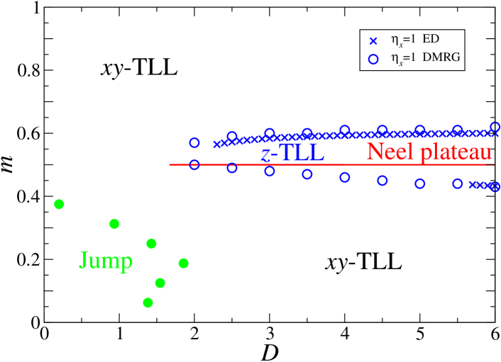
Figure 12: Phase diagram with respect to the anisotropy $D$ and the magnetization $m$. The crossover lines between the incommensurate parallel spin correlation dominant Tomonaga-Luttinger liquid ($z$TLL) phase and the Néel-like perpendicular correlation dominant one ($xy$TLL) are estimated by the numerical exact diagonalization (ED) (blue crosses) and the DMRG (blue circles). The phase boundary of the missing region because of the magnetization jump is estimated by the numerical exact diagonalization for $L=16$ (green circles). The Néel plateau is realized just on the red line.

VIII Summary

The magnetization process of the $S=1$ antiferromagnetic chain with the easy-axis coupling anisotropy and the easy-plane single-ion anisotropy is investigated using the numerical diagonalization for finite-size clusters and the DMRG calculations. It is found that the translational symmetry broken magnetization plateau appears at half the saturation magnetization for very large anisotropies (both of $\lambda$ and $D$). This explains the reason why this plateau has not yet been found in the $S=1$ chain compounds without the dimerization.maximova Several typical magnetization curves are also presented. Then, the effective theory constructed for $D\gg\lambda$ well explains the numerical results in Fig. 7. Nevertheless, an effective theory for the $D\ll\lambda$ case and the magnetization jump is a future problem. In addition, it is shown that the unconventional incommensurate parallel spin correlation dominant ($\eta_{x}>\eta_{z}$) Tomonaga-Luttinger liquid phase also appears around the 1/2 plateau as in Fig. 12. This situation is very natural because the condition for the realizationTLL of the Néel state ($|\cdots 101010\cdots\rangle$) is both of $\eta_{x}>\eta_{z}$ and the commensurability which is satisfied only at $m=1/2$.

In the previous work,yamada we investigated the half-plateau problem of a similar model but with $S=2$ to obtain the phase diagram which was much richer than Fig. 7 of this paper. In fact, the Haldane plateau phase and the large-$D$ plateau phase appeared in the $S=2$ case. This is because the half plateau is possible without the spontaneous breaking of the translational symmetry for the $S=2$ case. Namely the condition (1) can be satisfied by $Q=1$, $S=2$, $\tilde{m}=1$ (note that $\tilde{m}=1$ for the half plateau of the $S=2$ chain).

From the experimental point of view, one can usually expect a weak interchain interaction, which may induce the spin order corresponding to the most dominant correlation at a low but finite temperature. The phase diagram of Fig. 12 suggests that the incommensurate-SDW order associated with the $z$TLL can be realized around the $m=1/2$ plateau in the broad parameter region. Thus, such an enhancement of the SDW order could be a signature of the $m=1/2$ plateau due to the Néel-type mechanism, even if the width of the plateau is very narrow. We believe that the phase diagrams of Figs. 7 and 12 will be a powerful guideline for searching or synthesizing quasi-one-dimensional materials with $S=1$ which exhibit the half plateau without the dimerization.

- (1) for a review, T. Giamarchi, Quantum Physics in One Dimension, (Clarendon Press, Oxford, 2003).
- (2) E. H. Lieb, T. Schultz and D. J. Mattis, Ann. Phys. (N.Y.) 16, 407 (1961).
- (3) M. Oshikawa, M. Yamanaka and I. Affleck, Phys. Rev. Lett. 78, 1984 (1997).
- (4) T. Sakai and M. Takahashi, Phys. Rev. B 42, 4537 (1990).
- (5) A. Kitazawa and K. Okamoto, Phys. Rev. B 62, 940 (2000).
- (6) A. Honecker and A. Läuchli, Phys. Rev. B 63, 174407 (2001).
- (7) K. Okamoto, T. Tonegawa and M. Kaburagi, J. Phys.: Condens. Matter 15, 5979 (2003).
- (8) H. Kikuchi, Y. Fujii, M. Chiba, S. Mitsudo, T. Idehara, T. Tonegawa, K. Okamoto, T. Sakai, T. Kuwai, and H. Ohta, Phys. Rev. Lett. 94, 227201 (2005).
- (9) B. Gu and G. Su, Phys. Rev. B 75, 174437 (2007).
- (10) A. Honecker, S. Hu, R. Peters, and J. Richter, J. Phys.: Condens. Matter 23,164211 (2011).
- (11) N. S. Ananikian, J. Strečka, V. Hovhannisyan, Solid State Commun. 194, 48 (2014).
- (12) K. Morita, M. Fujihala, H. Koorikawa, T. Sugimoto, S. Sota, S. Mitsuda, and T. Tohyama, Phys. Rev. B 95, 184412 (2017)
- (13) Y. Ueno, T. Zenda, Y. Tachibana, K. Okamoto and T. Sakai, JPS Conf. Proc. 30, 011085 (2020)
- (14) R. R. Montenegro-Filho, F. S. Matias, and M. D. Coutinho-Filho Phys. Rev. B 102, 035137 (2020)
- (15) K. Hida, J. Phys. Soc. Jpn. 63, 2359 (1994).
- (16) K. Okamoto, Solid State Commun. 98, 245 (1996).
- (17) K. Okamoto and A. Kitazawa, J. Phys. A: Math. Gen. 32, 4601 (1999).
- (18) S.-S. Gong, B. Gu, and G. Su, Phys. Lett. A 372, 2322(2008).
- (19) G.-H. Liu, W. Li, W.-L. You, G. Su, and G.-S. Tian, J. Mag. Mag. Mat. 377, 12 (2015).
- (20) S.-S. Gong and G. Su Phys. Rev. B 78, 104416 (2008).
- (21) S. Mahdavifar and J. Abouie, J. Phys.: Condens. Matter 23 246002 (2011).
- (22) J.-J. Jiang, Y.-J. Liu, F. Tang, C.-H. Yang, Y.-B. Sheng, Commun. Theor. Phys. 61, 1 (2014).
- (23) X.-Y. Deng, J.-Y. Dou, G.-H. Liu, J. Mag. Mag. Mat. 392, 56 (2015).
- (24) T. Sugimoto, M. Mori, T. Tohyama, and S. Maekawa Phys. Rev. B 97, 144424 (2018).
- (25) T. Sugimoto, M. Mori, T. Tohyama, and S. Maekawa, Phys. Rev. B 92, 125114 (2015).
- (26) T. Sugimoto, M. Mori, T. Tohyama, and S. Maekawa, Phys. Rev. B 97, 144424 (2018).
- (27) K. Sasaki, T. Sugimoto, T. Tohyama, and S. Sota, Phys. Rev. B 101, 144407 (2020).
- (28) Sk. S. Rahaman, M. Kumar, and S. Sahoo, arXiv:2304.12266v2.
- (29) D. C. Cabra, A. Honecker and P. Pujol, Phys. Rev. Lett. 79, 5126 (1997).
- (30) K. Okamoto, M. Sato, K. Okunishi, T. Sakai, and C. Itoi, Physica E 43, 769 (2011).
- (31) R.-. Li, S.-L. Wang, Y. Ni, K.-L. Yao, and H.-H. Fu, Phys. Lett. A 378, 970 (2014).
- (32) Raphael C.Aćio, M. L. Lyra, and J. Strečka, J. Mag. Mag. Mat. 417, 294 (2016).
- (33) A. Farchakh, A. Boubekri, and M. El. Hafidi, J. Low Temp. Phys. 206, 131 (2022).
- (34) L. Yin, Z. W. Ouyang, J. F. Wang, X. Y. Yue, R. Chen, Z. Z. He, Z. X. Wang, Z. C. Xia, and Y. Liu Phys. Rev. B 99, 134434 (2019).
- (35) D. Dey, S. Das, M. Kumar, and S. Ramasesha, Phys. Rev. B 101, 195110 (2020).
- (36) S. Yamamoto and T. Sakai, Phys. Rev. B 62, 3795 (2000).
- (37) T. Sakai and K. Okamoto, Phys. Rev. B 65, 214403 (2002).
- (38) T. Tonegawa, T. Sakai, K. Okamoto and M. Kaburagi, J. Phys. Soc. Jpn. 76, 124701 (2007).
- (39) A. S. F. Tenório, R. R. Montenegro-Filho, and M. D. Coutinho-Filho, J. Phys.: Condens. Matter 23. 506003 (2011).
- (40) G.-H. Liu, L.-J. Kong, J.-Y. Dou, Solid State Commun. 213-214, 10 (2015).
- (41) K. Karlová, J. Strečka, Physica B 536, 494 (2018).
- (42) H. Yamaguchi, T. Okita, Y. Iwasaki, Y. Kono, N. Uemoto, Y. Hosokoshi, T. Kida, T. Kawakami, A. Matsuo,and M. Hagiwara, Sci. Rep. 10, 9193 (2020).
- (43) D. C. Cabra, A. Honecker, and P. Pujol, Phys. Rev. Lett. 79, 5126 (1997).
- (44) D. C. Cabra, A. De Martino, A. Honecker, P. Pujol, and P. Simon, Phys. Lett. A 268, 418 (2000).
- (45) W. Chen, K. Hida and B. C. Sanctuary, Phys. Rev. B 63, 134427 (2001).
- (46) Y. Narumi, K. Kindo, M. Hagiwara, H. Nakano, A. Kawaguchi, K. Okunishi, and M. Kohno, Phys. Rev. B. 69, 174405 (2004).
- (47) for a review of chain compounds, O. V. Maximova, S. V. Streltsov, and A. N. Vasiliev, Critical Reviews in Solid State and Materials Sciences, 46:4, 371 (2021).
- (48) X. Yan, W. Li, Y. Zhao, S.-J. Ran, G. Su, Phys. Rev. B 85, 134425 (2012).
- (49) K. Totsuka, Phys. Rev. B 57, 3454 (1998).
- (50) K. Okunishi and T. Tonegawa, J. Phsy. Soc. Jpn. 72, 479 (2003).
- (51) K. Okunishi and T. Tonegawa, Phys. Rev. B 68, 224422 (2003).
- (52) A. Metavitsiadis, C. Psaroudaki, and W. Brenig, Phys. Rev. B 101, 235143 (2020).
- (53) H. Nakano and M. Takahashi, J. Phys. Soc. Jpn. 67, 1126 (1998).
- (54) N. Okazaki, J. Miyoshi and T. Sakai, J. Phys. Soc. Jpn. 69, 37 (2000).
- (55) N. Okazaki, K. Okamoto and T. Sakai, J. Phys. Soc. Jpn. 69, 2419 (2000).
- (56) A. Nakasu, K. Totsuka, Y. Hasegawa, K. Okamoto and T. Sakai, J. PHys.: Condens. Matter 13, 7421 (2001).
- (57) T. Sakai and Y. Hasegawa, Phys. Rev. B 60, 48 (1999).
- (58) K. Okamoto, N. Okazaki and T. Sakai, J. Phys. Soc. Jpn. 70, 636 (2001).
- (59) K. Okamoto, N. Okazaki and T. Sakai, J. Phsy. Soc. Jpn. 71, 196 (2002).
- (60) F. Michaud, T. Coletta, S. R. Manmana, J.-D. Picon, and F. Mila, Phys. Rev. B 81, 014407 (2010).
- (61) H. Kohshiro, R. Kaneko, S. Morita, H. Katsura, and N. Kawashima Phys. Rev. B 104, 214409 (2021), and refereces therein.
- (62) T. Yamada, R. Nakanishi, R. Furuchi, H. Nakano, H. Kaneyasu, K. Okamoto, T. Tonegawa and T. Sakai, JPS Conf. Proc. 38, 011163 (2023).
- (63) M. P. Nightingale:, Physica A 83, 561 (1976).
- (64) K. Okamoto and K. Nomura, Phys. Lett. A 169, 433 (1992).
- (65) K. Nomura and K. Okamoto, J. Phys. A: Math. Gen. 27, 5773 (1994).
- (66) Z. L. Berezinskii: Sov. Phys. JETP 34, 610 (1971).
- (67) J. M. Kosterlitz and D. J. Thouless: J. Phys. C 6, 1181 (1973).
- (68) J. V. José, 40 Years of Berezinskii-Kosterlitz-Thouless Thoery (World Scientific, 2013).
- (69) G.-H. Liu, W. Li, W.-L. You c, G. Su, and G.-S. Tian, Solid State Commun. 166, 38 (2013).
- (70) N. Maeshima, K. Okunishi, K. Okamoto and T. Sakai, Phys. Rev. Lett. 93, 127203 (2004).
- (71) J. L. Cardy, J. Phys. A: Math. Gen. 17, L385 (1984).