Making Distribution State Estimation Practical: Challenges and Opportunities

Abstract

In increasingly digitalized and metered distribution networks, state estimation is generally recognized as a key enabler of advanced network management functionalities. However, despite decades of research, the real-life adoption of state estimation in distribution systems remains sporadic. This systematization of knowledge paper discusses the cause for this while comparing industrial and academic experiences and reviewing well- and less-established research directions. We argue that to make distribution system state estimation more practical and applicable in the field, new perspectives are needed. In particular, research should move away from conventional approaches and embrace generalized problem specifications and more comprehensive workflows. These, in turn, require algorithm advancements and more general mathematical formulations. We discuss lines of work to enable the delivery of tangible research.

I Introduction

The distribution networks (DNs) in countries like Germany and The Netherlands are already feeling the impact of the energy transition, as they face congestion for hundreds to thousands of hours per year because of the rollout of rooftop solar, EVs, and loads like data centers [1]. This drives a need for real-time visibility of the DN state and congestions.

I-A State Estimation and its Roots

In its standard textbook form [2], power system state estimation (SE) is a statistical monitoring method that combines exact network models and noisy electrical measurements to calculate the most likely state of the system, i.e., the minimum set of independent variables that fully describe the system’s steady-state physics at a certain moment in time.

The first real-time transmission system monitoring attempts directly read measurements from the supervisory control and data acquisition (SCADA) system [3]. However, this had limited success due to individual measurements’ noisy and unreliable nature. SE collates the different measurements, resulting in a reduced-noise, consistent and more reliable monitoring system that generates more information than the SCADA [3]. SE established itself as the industrial practice in transmission system control rooms in the 1970s - following the cornerstone work by Schweppe et al. [4].

In its present industrial implementation, transmission system SE (TSSE) is close to the textbook form; it is static, and it presents a refresh rate of a few minutes. In addition to noise filtering, TSSE primarily 1) estimates variables that are not measured directly, 2) detects, identifies and handles bad data, 3) detects and identifies unreported topological changes (e.g., switch states), and 4) provides input states to several energy management system (EMS) functionalities, such as contingency analysis and real-time markets or economic dispatch.

While its adoption dates back to around 50 years ago, TSSE is still an active research field, and industrial implementations may underperform. The NERC identified loss of TSSE as the main source of EMS malfunction [5]. Gou and Shue [6] recently wrote on the challenges of industrial TSSE solutions.

I-B Changing Perspectives on SE in Distribution Networks

Distribution system SE (DSSE) literature only appeared about two decades after Schweppe’s work [7], when it became clear that distribution network (DN) management was becoming increasingly active and thus required monitoring.

There has been general consensus that, given the differences between transmission and distribution systems, DSSE methods must differ from TSSE. Of the four primary use cases of TSSE defined in the previous section, 1) still applies to DSSE, and is tied to the mathematical definition of SE. 2) and 3) are desirable, but existing TSSE techniques might not work for DSSE, given the scarcity of measurements and generally slow sampling rates. Moreover, 2) and 3) are very sensitive to errors in network models, which are common in DNs. These impact the SE residuals, making the handling of bad data and anomalous topology difficult if approached with TSSE-like residual analysis [2, 8]. Use-case 4) is of interest and possible for DNs. However, given the limited and ‘slow’ measurements (which are also often averaged - as opposed to instantaneous), and few automated assets, the target EMS applications will differ from TSSE’s, at least in the near future.

I-C Data Quality Issues Demand Parameter Identification

Network models for TSSE are considered trustworthy, and bad data detection and handling refers to measurement data. In DNs, the opposite is common: utilities tend to trust the (few) available sensors while network models are considered untrustworthy and error-prone. The presence of errors in DN models is recognized both by industry and academia [9, 10].

These network parameter errors affect DSSE in a fashion that is somewhat similar to bad measurements (i.e., they increase the residuals), but are more pervasive, persist over time (until the DN model is adapted) and change over time (unreported system changes due to operations and maintenance). Conventional SE residual analysis struggles to differentiate between incorrect network model parameters and noisy measurements. A recent DSSE validation on a real DN illustrates that the large normalized residuals method may flag acceptable current measurements as bad data due to relatively modest impedance modeling errors [8]. As there are more potential error sources in DNs than the transmission system, calibrating DN models requires more expertise and time.

Modern DN computation toolboxes, e.g., OpenDSS [11], PowerModelsDistribution [12] and PowerGridModel [13], support increasingly sophisticated models, e.g., explicit-neutral four-wire. However, their results are only as reliable as the input data used. The creation of DN models that accurately represent reality is needed to unlock the full potential of digital twins.

While conventional residual analysis might not always be effective, we posit that it is possible to exploit DSSE to build, improve and validate DN models. Even more so, we believe that the maximal benefit from DSSE, from an industrial standpoint, rests in such model building tasks. This entails a paradigm shift, which consists of seeing state and parameter estimation as part of the same problem, as opposed to two disjoint problems, and is extensively discussed in this paper.

I-D Scope and Contributions

This work contextualizes and conceptualizes the problem space surrounding static DSSE, focusing on the applied industrial perspective. We observe that improvements needed in industry are far from mere pragmatic adjustments and require non-trivial theoretical and algorithmic advancements. We discuss the issue of making DSSE more practical by untangling some muddled terminologies, problem descriptions, and modeling approaches in the distribution system state and parameter estimation field. We aim to inform and inspire researchers working on power system optimization methods to bridge the gaps and bring solutions to the field.

Alternative DSSE approaches exist, e.g., based on machine learning [14], or dynamic filters [15]. Their discussion is out of scope as we focus on model-based static DSSE.

The paper is structured as follows. First, we discuss the problem statements from the power flow (PF)/SE perspective compared to parameter estimation (PE) (§II). We review existing work on PE for DNs and find that it is often not integrated with DSSE (§III). We then discuss the algorithmic advancements needed to enable practical and advanced DSSE (§IV). Next, we address practical challenges in DSSE deployment and the development of digital twins (§V). Finally, §VI summarizes and concludes the work.

II DSSE, related problems and misconceptions

We first discuss widely-accepted problem specifications of PF, DSSE and related problems, and their inverses.

II-A Power Flow, State Estimation & Load Allocation

Power flow is a mathematical problem that solves circuit physics while satisfying load/generation set points in active/reactive power given a reference bus. PF contains non-convex equalities from AC network constraints, necessitating nonlinear root-finding methods like the Newton-Raphson or fix-point iteration algorithms [16].

Conceptually, SE generalizes PF. Voltage measurements from any bus can be used directly in SE, whereas a PF can only accommodate complex voltage at the reference bus and voltage magnitude at generator buses. Other types of measurements can also be leveraged (e.g., relative and/or absolute voltage angles), as long as the corresponding functions define the measurement quantities in terms of the state variables.

In the context of DNs, both PF and SE should model phase unbalance (and neutral voltage in four-wire DNs) [17, 18], and symmetrical components should be avoided [18]. While the proposed modeling effort is not hard to support when building models and solvers from the ground up, re-purposing or adapting existing transmission-focused approaches and software solutions is practically intractable.

Load allocation (LA) is related to SE and PF, and typically conceived on top of a PF engine. LA aims to set up a realistic time simulation model of the system by assigning and dividing aggregated loads to a set of buses in the network [19]. Practitioners then validate their model by looking at voltage and power at the substation but typically have no other measurement data available to assess the LA quality.

II-B States vs. Variables vs. Parameters

Conventionally, for the (static) power system SE problem, complex nodal voltages are taken as the only unknowns and are represented in a stacked fashion in the ‘state variable vector’. This restrictive definition excludes transformer taps (and other parameters). However, taps may change in the field based on local control loops, and thus their estimation/tracking may improve the quality of the results. Table I summarizes the features of relevant PE problems.

TABLE I: Parameter estimation categories.

Category	Specific parameters	Problem statement	Nature
Topology	Topology detection	Obtain list of energized lines/cables given a trustworhy graph	discrete
	Topology estimation (green-field)	Given a set of connected buses, estimate the graph	discrete
	Topology estimation (incremental)	Given a graph, fix the connectivity errors. Includes switch state estimation.	discrete
	Phase connectivity identification	Estimate phase connectivity, usually given meter-to-transformer/feeder assignment	discrete
	Meter-to-transformer assignment	Find to which transformer a user/meter is connected	discrete
Line	Impedance estimation	Infer line impedance matrices	continuous *
	Line type estimation	Select most likely construction code from a set of construction codes	discrete
	Line properties estimation	Estimate most likely temperature, line spacings, radius, material types	mix
Transformer	Impedance estimation	Estimate transformer loss terms	continuous
	Transformer tap position	Estimate tap position of the transformer	discrete
	Transformer type	Estimate the type of transformer (wye-wye, delta-wye, center-tap)	discrete
Regulator /	Gang vs per-phase operation	Categorize whether taps are locked together or not	discrete
OLTC	Impedance estimation	Estimate impedances in equivalent circuit	continuous
	Controller mode estimation	Categorize hysteresis vs line-drop compenstation, etc.	discrete
	Bidirectional capable?	Estimate whether controller operates correctly under reverse flows	discrete
PV system	Rating estimation	Estimate ratings of panels and inverter	continuous
	Control mode identification	Categorize constant PF vs volt-var/watt	discrete
	Control setting estimation	Estimate volt-var/watt curve values	mix

In typical DSSE implementations, the Jacobian (and Hessian) derivative expressions are hard-coded, and adding new state variables requires adaptation of these matrices, which is error-prone. Relying on modern optimization frameworks that support automatic differentiation enables faster prototyping. However, much of the current research in power grid state estimation does not consider progress being made in the applied mathematics or operations research community. In this context, we observe that a majority of the leading teams of the ARPA-E Grid Optimization Competition resort to the same or similar underlying NLP algorithm implementations [20], e.g. the open-source solver Ipopt or KNITRO.

II-C Forward and Inverse Problems

In the literature, parameter estimation problems for power networks have been discussed under various labels:

• system or parameter identification or estimation;

• generalized or augmented state estimation;

• inverse power flow problem.

In the literature, the terms are used interchangeably, e.g. [21, 22, 23]. Here we use ‘parameter estimation’ as the overarching term to indicate the concept. For individual parameters, we stick to the continuous/discrete considerations.

To minimize semantic confusion, we use terminology inspired by the language in the operations research community:

• parameters: representing knowns in the mathematical model, i.e., inputs supplied to the engine;

• variables: representing unknowns in the mathematical model, i.e., results calculated by the engine.

Mathematically speaking, the inverse problem of a (forward) problem consists of recasting all parameters as variables and vice-versa in the postulated system of equations. However, most authors only involve the continuous parameters/variables in this swapping operation, as making discrete parameters into variables may trigger the problem to become combinatorial in nature. As PF and SE are generally considered continuous problems, when postulating their inverse, the discrete inputs - i.e. the topology - are typically kept as-is. Nevertheless, this restriction can be dropped, with authors investigating discrete topics like topology identification (TI).

Table II summarizes the variables and parameters as defined in canonical PF and SE problems, and illustrates continuous and continuous+discrete generalizations. Potentially, all symbols appearing in the equations of the mathematical model may become variables. In such case, the only model parameters (inputs) are the measurements, and we end up intersecting SE, PF and OPF with their own inverses. However, the challenge of exploiting the mathematical structure where all symbols are variables is that the overfitting risk increases. Authors that address joint DSSE and PE often assume a fixed topology (except perhaps a few variables), and thus the problems retain largely continuous features, whereas TI problems abstract on continuous variables so that they are purely combinatorial.

TABLE II: Canonical problem specifications and beyond

			Canonical power flow		Canonical state estimation		Generalized cont.	Generalized
	Quantity	Symbol	Forward	Inverse	Forward	Inverse	Combined	Combined
Discrete	Line connectivity	$(l,i,j)\in\mathcal{T}$	param.	param.	param.	param.	param.	var.
	Load connectivity	$(d,i)\in\mathcal{T}^{d}$	param.	param.	param.	param.	param.	var.
	Generator connectivity	$(g,i)\in\mathcal{T}^{g}$	param.	param.	param.	param.	param.	var.
Continuous	Bus voltage	$U_{i}$	var.	param.	var.	param.	var.	var.
	Line impedance	$Z_{l}$	param.	var.	param.	var.	var.	var.
	Load value	$S_{d}$	param.	var.	var.	param.	var.	var.
	Generator value	$S_{g}$	param.	var.	var.	param.	var.	var.
Extensions	TF tap ratio	$T_{l}$	param.	param.	param.	param.	var.	var.
	Those listed in Table I		-	-	-	-	var.	var.
	Variable bounds		-	-	-	-	$\checkmark$	$\checkmark$
Math.	Class		Nonl. root-find.	NLP	Nonl. WLS	NLP	NLP	MINLP
complexity	Algorithm		NR	IP	GN	IP	IP	custom

We note that Yuan et al. [24] defined the inverse PF problem as: “the estimation of the nodal admittance matrix from synchronized measurements of voltage and current phasors”. As per our mapping, that would be more precisely described as the inverse state estimation problem. Note that the generalization hierarchy reverses: SE generalizes PF in the forward space, and viceversa in the inverse space.

The scope of any problem can be increased, e.g., by adding new variables (like taps in SE), or by allowing new mathematical structures such as variable bounds. Once an engine is built for a stated problem specification, it is often feasible to re-cast variables as parameters, while the opposite would increase the complexity and might be impractical.

When PE is performed, it is often crucial to exploit time series, so the generalized problems need to be conceived of as fundamentally multiperiod: assuming parameter values to be time-independent helps manage the overfitting risk.

II-D Uniqueness and Observability

From a mathematical/control theory standpoint, observability for a steady-state system $S$ requires a one-to-one mapping between measurements and states in a noiseless environment. Given a measurement vector $z$, states $x$, and noise vector $n$ for some system $S$, observability holds if, for a noiseless scenario $n=0$, we can recover $x$ from $z$ uniquely. Local observability is less strict and can be met if, within a small operating neighborhood of system $S$, there is a unique $x$ to $z$ mapping in a noiseless scenario. Full-rank conditions, as generally used in power systems SE, can satisfy local observability.

Uniqueness, in the context of root-finding, requires a unique mapping between an arbitrary system of nonlinear equations $F(x)$ and $x$, in some interval $(\overline{x},\underline{x})$. Uniqueness issues exist:

• PF generally does not have a unique solution, but in some practical intervals of states this can be the case (e.g., high-voltage solutions).

• SE is unique in observable linear systems. In nonlinear ones, generally only local observability can be achieved.

• Sometimes SE is only locally partially observable; here, only some states $x_{o}\subset x$ can be estimated given a set of limited measurements $z_{o}$.

• LA is generally not unique. If performed with a SE engine, the SE considerations hold.

• Nodal admittance matrices are usually unobservable; careful construction achieves local observability [24]. Other than [24], observability and uniqueness are rarely formally discussed for PE.

The industrial view is that uniqueness is not that interesting, unless it leads to wrong outcomes, i.e., losing extrapolation value. Out-of-sample testing is a good strategy to build confidence in models that are not guaranteed to be unique.

II-E Error and Uncertainty Sources

Existing implementations of DSSE and PF platforms suffer from inaccuracies across different data sources [9]:

• modeling errors or shortcuts due to applying the circuit laws under invalid assumptions, e.g., use of Kron’s reduction in sparsely grounded networks.

• network data errors, e.g., wrong topology information;

• (largely) inevitable measurement errors: ‘noisy’ or ‘bad’ data due to sensor tolerances or malfunction; and

• measurement inadequacy due to 1) semantic mismatch, e.g., having averaged instead of instantaneous rms values, 2) granularity mismatch, e.g., aggregated three-phase measurements instead of per-phase; 3) label mismatch, e.g., wrong location or phase meta-data, 4) measurements that are not adequately synchronized.

Inherently, any error adds to the SE residuals, and distinguishing model error, network data error and measurement error is nontrivial. Potential solutions include:

• flexible models with variables to represent alternative states, e.g., neutral conductor breakage;

• exploiting time-independence.

The cost to investigate data issues by human inspection may be prohibitive, and data-driven methods help decrease that effort. However, if only power measurements are available, it is unrealistic to reliably discover network parameters: voltage is necessary for validation. In the presence of network errors, the increased residuals may not reconcile, and some SE methods may diverge [2] (chap. 8). Nevertheless, DSSE, contrary to PF, can be leveraged to calibrate network models.

III State and parameter estimation

In the presence of pervasive network errors, a first, thorough offline PE is arguably necessary, using historical measurements to derive a DN model as close to the present-state reality as possible. However, this is not sufficient: as power systems change over time, DN data sets should be self-correcting, and such corrections should occur as close to real-time as possible. Fig. 1 summarizes our vision for the data flows between measurement and DN data sources towards the SE, indicating the types of data issues that may appear throughout.

Figure 1: State estimation as part of overall architecture. Novel information flows related to parameter identification indicated bold.

From here on, we refer to the first offline PE as ‘historical’ (HIS), and to the subsequent ‘on the run’ corrections as ‘near-real-time’ (NRT). Different specifications emerge in the two contexts; e.g., time-independence of properties might be exploitable in HIS  but not in NRT. Table I provides a summary of parameters to be estimated, including less common ones.

III-A Notes on Topology Identification

Deka et al. [26] classify topology learning into topology ‘detection’ and ‘identification’, which is an important distinction as different methods are used to solve the two. The former assesses which lines are energized and which not, assuming their impedances and locations are known, and can be approached with model-based methods. The latter consists of the green-field reconstruction of the whole connectivity model, (possibly) including line impedances, and is a high-dimensional combinatorial problem. Thus, it is usually addressed with techniques that abstract from the power flow physics, e.g., graph learning [22, 27]. This paper primarily focuses on model (power flow equations) based solutions. Thus, we focus on TI in its detection declination. Interested readers can refer to [26] for a thorough survey of TI methods.

III-B State and Parameter Estimation Literature

Table III provides a selection of PE references. This is not exhaustive: the objective of this paper is to discuss the main ideas behind the methods, not to provide a complete review.

State and parameter estimation can be performed sequentially, jointly, or disjointly.

The ‘sequential’ approach was the first to be proposed in the context of integrating PE as part of static SE workflows (although still used in recent literature [28]), and is based on the statistical analysis of SE residuals. First, SE is performed (on one snapshot). Then, the residuals are analyzed in search of anomalies that can be attributed to unreported changes or other localized errors, e.g., a wrong line impedance. This concept has been applied particularly in a NRT context, as $1)$ SE is originally designed as a real-time operational tool, and measurement history is not stored, and $2)$ in NRT only few errors are expected (e.g., few switch state changes): a diffused presence of errors would pervasively increase residuals, compromising their statistical analysis. In equality-constrained SE, Lagrangian multipliers can replace residuals.

The joint presence of bad data and network errors is also likely to compromise residual analysis. The NYSERDA report [29] identifies the distinction between bad data and inaccurate network models as a key challenge to real-life DSSE. Measurement scarcity is an additional challenge [29, 30]. Multi-period problems are known to balance lower measurement redundancy levels [2] (Section 7.7), and thus appear more promising for DSSE. Comparing the residuals of separate successive SE calculations, without setting up a real multi-period problem has also been investigated [31, 32]. Multi-period implementations are possible with both joint and disjoint approaches, and produce automated results.

‘Joint’ state and parameter estimation has existed for several decades for continuous parameters, and is also known as ‘state (vector) augmentation’ [2]. Over the years, multiple parameters has been incorporated: multi-conductor impedances [33, 34], zero-impedance branches [35], switch [36, 37] or breaker [38] states, tap settings, modeled either continuous [39, 40] (with rounding), or discrete [41].

TABLE III: Parameter estimation literature. -: not addressed, as far as the authors know. Red indicates multi-period problems.

Category	Parameter	Joint		Disjoint		Sequential
		HIS	NRT	HIS	NRT	HIS	NRT
Topology	Topology detection	-	[36, 42]	[43]	[44]	-	[2, 45]
	Topology estimation (green-field)	-	-	[26]	[46]	-	-
	Topology estimation (incremental)	-	-	-	-	-	-
	Phase connectivity identification	[47]	[47]	[48, 49]	-	-	-
	Meter-to-transformer assignment	-	-	[50, 51]	-	-	-
Line	Impedance estimation	[33]	-	[52, 53]	-	-	[2, 32]
	Line type estimation	-	-	[54]	-	-	-
	Line properties estimation	-	-	-	[55]	-	-
Transformer	Impedance estimation	-	[56]	-	[57, 58]	-	-
	Transformer tap position	[34]	[41, 39, 40]	-	-	-	[59]
	Transformer type	-	-	-	-	-	-
Regulator/OLTC	Gang vs per-phase operation	-	-	[60]	-	-	-
	Other (impedance, control…)	-	-	-	-	-	-
PV system	PV rating estimation	-	-	[61]	-	-	-
	PV control mode identification	-	-	-	-	-	-
	PV control setting estimation	-	-	[62]	-	-	-

Augmenting the state to incorporate discrete parameters would lead to mixed-integer non-convex programming problems, which are prone to scalability issues. Relaxations and approximations of non-convex constraints have led to tractable yet effective mixed-integer problems. These are relatively common in the context of joint SE and topology detection, e.g., [36], but are nearly non-existent for phase identification: deriving the connectivity of all users results in a large number of binary variables, and to our knowledge, the only mixed-integer SE augmentation for phase connections is [47].

While all modeling errors usually increase the residuals, inaccurate impedances generally cause much lower increases than wrong discrete parameter values [2, 47]. This can be exploited, e.g., first to estimate discrete variables, fix them, and then subsequently perform impedance estimation [47].

‘Disjoint’: PE is performed without using SE concepts, usually in an HIS manner. Phase identification is almost exclusively performed disjointly, most often via voltage measurements clustering [48], although power measurements can be used [49], and the same holds for green-field TI [26]. Several researchers estimate cable impedances with linear regression [63, 64, 54]. Yusuf et al. [60] present data-driven methods to identify the tap position of voltage regulators and establish whether the tap changers are phase- or gang-operated. Gotti et al. [44] and He et al. [43] use DSSE to validate topologies estimated in a disjoint manner.

Note that topology detection is usually limited to detecting switch states when it is done jointly with or sequentially after DSSE. TI methods (or adaptations) could perform ‘incremental TI’, i.e., sparse connectivity errors that do not correspond to switch locations. These data quality issues exist in real network data [9] but are not addressed in the literature. Topology, line parameters, and tap settings appear well investigated, whereas limited work addresses other transformer/regulator parameters. In particular, transformer types and groups are assumed to be known, while in our industrial experience this is not the case. Transformer models are defined by winding resistances, leakage inductance, shunt properties, etc. Data-driven estimation methods exist [65], which do not require disconnection. However, transformer parameter estimation is performed with ‘local’ measurements only, e.g., voltages and currents at the transformer terminals, and not as part of a ‘full’ augmented DSSE, except in [56]. However, [56] only estimates turns ratio and series impedance. A few references are gathered in Table III as ‘Transformer - impedance estimation’. Notably, most papers address single-phase transformers only.

Finally, most - if not all - existing PE methods implicitly assume that the users/meters are assigned to the correct transformer (beforehand). If this is not the case, the successive estimation process is compromised. Researchers have only recently addressed the data-driven association of meters to the correct transformers. While the literature is limited, various names are used, e.g., ‘transformer-customer relationship identification’ [50], or ‘meter-transformer mapping’ [51] (M2T).

III-C Behind-The-Meter Resource Estimation

Parameter estimation typically refers to network asset properties, however, parameters of behind-the-meter (BTM) resources are often unknown and assuming certain properties may significantly impact grid analytics and monitoring [66]. The identification of BTM parameters is a novel research topic and has not been explored in the context of augmented SE, even though for some parameters this might be possible.

In contexts where smart meters (SMs) are not bidirectional, disaggregation of demand and PV generation is essential. Existing approaches are reviewed in [66]. Like for DN PE, these can be model-based, fully data-driven, or a combination.

Where SMs are bidirectional, grid injections may be directly measured (although self-consumption may still be unaccounted for), but inverter control settings and energy management behavior are still usually unknown.

Most methods for PV require or are facilitated by the use of exogenous information, such as irradiance [66], although methods based only on electrical measurements exist [61, 62]. Mason et al. [61] present a supervised learning model for size, azimuth and tilt estimation of PV installations based on net power data. Talkington et al. [62] disaggregate demand and generation and derive reactive power control settings (constant PF and Volt-var) of PV inverters, using historical power and voltage data. Voltage-only-based methods are also possible, if a good-quality secondary circuit model is available [10].

There is significantly more literature on PV disaggregation than control mode estimation, e.g., [67]. Similarly, the non-intrusive load modelling literature is also abundant [66], and techniques similar to [62] could be extended to other inverter-based resources, post disaggregation of the resource’s load. To our knowledge, there is no literature on the topic.

Additionally, the identification of PV control modes appears unaddressed, e.g., [62] assumes to know a-priori which inverters perform constant power flow control and which Volt-var. Similarly, identifying regulator control modes and bidirectional capabilities is industrially relevant but unexplored.

Finally, we note that the identification of load models (constant power, vs ZIP, etc.) is also beneficial, and has received academic attention [66].

IV Necessary Algorithmic Advancements

We now discuss algorithmic bottlenecks of DSSE generalizations. We posit a need to move beyond Gauss-Newton (GN) and WLS when the following are desired:

• non-Gaussian state estimation (both in a robust sense and in a best estimator sense);

• conditional estimation;

• joint state and parameter estimation;

We argue that all are crucial to make DSSE practical.

IV-A Gauss-Newton and Other Algorithms

Newton-Type WLS Algorithms: The most common solution technique for SE is the GN algorithm [68, 69] (§V.A), a Quasi-Newton method that is applicable to least squares minimization problems. GN approximates the Hessian from the Newton-Rhapson (NR) method in its iterations, making it less robust than NR. Furthermore, it cannot naturally incorporate variable bounds or inequalities. Nonetheless, by avoiding the calculation of the Hessian, GN is generally assumed to require less computation per iteration than NR.

The incorporation of very diverse weights for different measurement types in DSSE, particularly pseudo-measurements (very low weights) and zero-injection buses (very high) results in ill-conditioning. Improvements on the basic GN-based implementation avoid using high weights for virtual measurements [70], modelling them as equality constraints and solving the Lagrangian [68]. Further extensions of these algorithms allow for SE in underobserved systems, where the gain matrix is rank-deficient and thus non-invertible [30].

NR has also been explored for constrained optimization-based SE, but much less frequently. NR can include any number of equality and inequalities, and (with heuristics) has better convergence for large-practical networks, which helps solve difficult instances. In practice, NR convergence significantly improves if i) the Hessian at each iteration is positive-definite, to ensure descent direction and ii) LS techniques are used to choose an appropriate step size to achieve sufficient objective improvement in each step. Due to its approximations, GN does not need routines to deal with non-PSD Hessians, but, as a consequence, LS may not be as powerful.

Trust-region algorithms: The Levenberg-Marquardt (LM) method, a kind of trust region method that applies to least-square minimization problems, improves on GN. LM interpolates between the GN and the method of gradient descent and is more robust than GN: it can generally find a solution even when the initial condition is far from the minimum. Moreover, it is more stable than NR as it ensures step-sizes within a trust region but generally converges slower than GN and NR.

Very little literature exists on trust region-based SE. Pajic and Clements [71] explore them for TSSE, together with GN with line search (LS), motivated specifically by improving reliability in the presence of bad data such as topology errors. They observe that the trust region approach is the most reliable in difficult conditions, e.g., the presence of cascade failures.

Nonlinear programming: Recently, NLP approaches have become popular [72, 17, 73, 74, 75, 76]. These can solve SE with both equality and inequality constraints. Inequalities can be used to model non-monitored users [72]. Algebraic modeling toolboxes with automatic differentiation 1) allow a clear separation between the model ( equations and objective) and the solver (e.g. Ipopt), 2) can support WLAV objectives naturally [77, 73], as the nondifferentiability of the objective function is avoided through reformulation using inequalities and the epigraph transform, and 3) facilitate alternative formulations of the circuit physics, e.g. through convex relaxations [78] or linear approximations. There is much less research on alternative formulations in the context of SE than OPF. Presumably, this is because any approximation implies modeling errors that add up to the residuals, making the decision support outcome measurably worse despite potential speedups. For PE, approximations may be acceptable, but when approximated SE and PE are performed jointly, a final nonconvex SE with the fixed parameters is recommended. Taheri et al. discuss using SE to recover feasibility of relaxed/approximated OPF models [79].

SE can also be approached with matrix completion, which consists of estimating missing values in low-rank matrices. Such methods are particularly well-suited for contexts with very limited observability [80], but most implementations rely on semidefinite programming (SDP) models [81, 82, 80, 83], which – despite their convexity – struggle to scale in practice. Specifically, the network feasibility in the SDP approach is inherently dependent on the solution being rank-1; which is rarely the case for larger networks. If the solution is not rank-1, a feasible AC solution cannot be recovered. Therefore, Liu et al. develop a more practical approach as a quadratic nonconvex optimization problem [84].

Other approaches: Cao et al. [85] give an overview of learning-based DSSE methods and propose one that can detect topological changes by including some physics. However, the rationale behind adopting a learning-based approach is that system parameters are unknown, which we argue to be an issue that should and can be solved instead.

Discussion: We posit that for large problems, especially those with multi-period constraints and many zero-injection nodes, NR approaches within constrained optimization SE frameworks are the more robust, i.e., most likely to converge.

Approaches that support inequality constraints allow for conditional SE: e.g., to establish a quality of the fit while requiring variables to be in a certain range. Furthermore, in GN, the objective must be a WLS function or variants such as a Schweppe-Huber. WLAV, however, is nondifferentiable, so it requires a different algorithm.

IV-B Maximum Likelihood Estimation

SE is a maximum likelihood estimation (MLE) problem that establishes realized values for random variables subject to a probability distribution. WLS minimization is the ‘correct’ MLE only if all measurements present white Gaussian noise. WLS corresponds to the $\ell_{2}$ norm, with strong theory and closed-form results. Different distributions have different maximum likelihood models [86]; for instance, the Laplace distribution maps to the $\ell_{1}$ norm, i.e., WLAV minimization. As a regularizer, $\ell_{1}$ is understood to induce sparsity much more than $\ell_{2}$, which makes the WLAV more robust. WLS is sensitive to outliers w.r.t. to alternatives, so it is sometimes deliberately replaced with objectives that are more robust:

• $\ell_{0}$ ‘norm’, a.k.a. measurement discarding, may identify sources of bad data but is combinatorial;

• the Schweppe-Huber function avoids nondifferentiability of WLAV, is less sensitive to outliers but typically nonconvex;

• the matrix nuclear norm as a proxy for rank in the context of matrix completion [80] is convex;

• mixing the above, with or without penalization.

V Real-World Experiences with DSSE

V-A Lessons Learnt From Collaborative R&D Projects

Bad data can only partially be managed through heartbeat protocols, watchdog timers and error correction codes. In addition to large random noise events, data adequacy issues and flawed sensor installations are common in practice:

• unknown or inconsistent measurement setup, e.g., phase-to-neutral vs phase-to-ground voltages,

• miswired voltage/current transformers (i.e. 180^∘ offset);

• wrongly accounted-for voltage/current transformer ratios;

• phase rotation order wrong;

• mislabeled units (e.g. kW vs W, V vs kV);

• measurement values reported are min/max over the interval, not the mean or median.

Some of these errors are expected to be caught promptly, e.g., when being used for billing purposes. During SE deployment, experimentation with error rejection strategies can be particularly useful as a mechanism for root-cause analysis. Finally, we observe that while they may not result in bad data, the following adequacy issues are detrimental to SE and/or PE:

• long measurement intervals, thereby underestimating spiky loads and network losses;

• only aggregate three-phase power measurement available, not individual phase or line values;

• measurement systems that only communicate new values when a (high) threshold for change is exceeded.

V-B Lessons Learnt At Alliander DNO

Alliander, the largest DN operator in The Netherlands, serving over three million customers, started in 2015 with the implementation of SE. Its MV and LV network consists of over 40 000 km of cable split up into 22 million segments.

The biggest technical challenges were developing a fast enough DSSE algorithm and preparing a suitable dataset for the entire DN. At the time, no marketed product could handle SE of this scale, so Alliander initiated the development of the PowerGridModel [13], which according to Xiang et al. [87], the fastest open-source SE toolbox currently available. Alliander follows a SE implementation pathway, with foreseen applications in increasing order of practical difficulty:

Improving topological network data: The first result of every practical SE attempt is finding errors in topological network data. In the case of Alliander’s dataset of 22 million cables, hundreds of thousands of errors were identified. The faults mainly consisted of short, missing LV cable sections, creating network areas seemingly disconnected to the main grid. Since many processes within a utility rely on accurate data, this is already a very valuable result. Most SE algorithms also give spatial information about mismatches between models and sensor information. This helps identify faulty sensors and unrealistic cable properties.

Optimizing sensor design and placement: Certain SE implementations can give the uncertainty of their estimated states. This is valuable information for adding sensors to the network, as they can be added to the places with the most uncertainty. Using simulations, it can also be estimated how much extra sensors improve the results of SE.

Real-time load modeling MV: Once data and sensoring are sufficient, SE is deployed, generating valuable information on network congestion and outages. It is advisable to start the practical implementation of SE on the MV network, as the LV network poses extra challenges.

Real-time congestion management: With clear real-time insight of the energy flows within the electricity network, techniques to control congestion can be explored.

Fraud detection: With near-perfect SE, detecting fraud is a possibility. However, given the cost of a false positive, it is probably infeasible to create an SE result that is good enough to use for fraud detection on its own.

The biggest non-technical challenge of implementing SE was keeping the algorithms explainable to non-technical colleagues. A metaphor that worked well is, ‘We are currently regulating traffic without knowing where the traffic is. SE will let us know where the traffic is in real-time.’. Alliander believes SE will be invaluable in finding and mitigating congestion, thus facilitating the energy transition.

V-C Lessons Learnt At Energy Queensland

Two DNs operate in the state of Queensland, Australia: Energex services the heavily populated southeast corner, and Ergon Energy Network the regional and remote northern parts. They connect 2.3 million customers with 212 000 km of powerlines and cables ranging from 132 kV to LV. Queensland DNs support almost 745 000 rooftop and other small-to-medium solar energy systems, with numbers steadily increasing. This triggered minimum demand situations, significant reverse flows, voltage performance issues and DN congestion. In 2019, these challenges prompted the implementation of DSSE to improve DN visibility using the limited telemetry available. Key lessons learned are:

Network Model: The term ‘network model’ means many things to many people. Network models used in other business contexts, e.g., operations and planning, shortcuts for simplifying visual representation, computation or hold only hierarchical associations, resulting in deficiencies in the detail required by DSSE. The Geospatial Information System (GIS), being the only source of LV network data, was deemed the primary network model data source for SE; however, the GIS is filled with connectivity issues, particularly at LV. One example is that customers are represented as being attached to a distribution transformer rather than the actual point of coupling to the LV DN. Improving field data capture and using SMs to infer connectivity improves DN data. MV is the initial focus of DSSE deployment due to the superior quality of available network models w.r.t. LV.

Telemetry: SMs are the responsibility of retailers and are used for billing purposes only, making access to SM power quality data difficult for DNs. The industry recognises the value of SM data for DN operations, but regulatory changes improving access take time. The rollout of monitoring on the LV side of MV/LV transformers has proved invaluable. Monitoring coverage of $\approx$30% has generally proven sufficient for accurate SE results (Fig. 2). Standards are being updated to improve telemetry from SCADA devices for SE. Limitations include aggregated three-phase power flows rather than individual phase measurements or measuring current magnitude rather than active and reactive power. Setting up data streaming capability to deliver telemetry to DSSE in NRT is fundamental to success and was achieved through Apache Kafka.

Cross-System Data Mapping and Naming Conventions: SE requires reconciling inputs from GIS, asset, customer, metering and SCADA data systems. Naming conventions are important to ensure objects (e.g., a transformer), asset characteristics (e.g., rating, tap position) and telemetry can be matched. Alignment is challenging when information is mastered in different source systems.

Early results show promise in delivering DSSE-derived ‘synthetic’ grid visibility data as distinguished from sensors. Power flows are not measured on most MV feeders making periods of reverse flow hard to identify. Currently, the DN utilities use CT data looking for a characteristic bounce at the zero crossing as an indication of likely reverse flow (Fig 2).

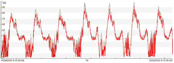
Figure 2: Out-of-sample validation of underobserved DSSE on an MV DN feeder in Queensland. The indicated quantity is current (A), the grey line is the DSSE solution, and the red line is measured.

Another key application of SE and subsequent network-constrained optimisation is to support dynamic connection of customer DERs [88]. Networks collaborate with customers to manage rooftop solar, electric vehicles and batteries by flexibly varying export and import limits at the point of coupling, informed by congestions made visible through DSSE. Educating engineers, field technicians and solution architects within the business on incremental no-regrets actions to establish a digital and data environment favourable to DSSE allows the opportunities to be realised sooner and more cost effectively.

VI Conclusions and Future work

This paper discussed the main technical bottlenecks and industrial misconceptions that hinder the adoption of state estimation in DNs. We argue that treating state and parameter estimation as a single problem, instead of two distinct ones, is a crucial step towards applicable solutions. This calls for the adoption of less conventional problem formulations and algorithms. Some examples exist in the literature, and have been reviewed here. We highlight specific research gaps where present, but stress that, in general, a change of perspective is required, e.g., including adaptive, automated and thorough network model cleaning pipelines. Finally, further benefits can be harvested through R&D on:

• exploration of synergies between data-driven and physics-based solutions for state and parameter estimation;

• root-cause analysis methods for network (data) issues;

• maximum likelihood and sparsity-inducing estimators combined with improved statistical models to detect meter configuration errors and other anomalies;

• implications of limited observability on decision risks.

References

- [1] E. Beckstedde and L. Meeus, “From “fit and forget” to “flex or regret” in distribution grids: Dealing with congestion in European distribution grids,” IEEE Power Energy Mag., vol. 21, no. 4, pp. 45–52, 2023.
- [2] A. Abur and A. G. Exposito, Power system state estimation: theory and implementation. CRC press, 2004.
- [3] S. Pajic, “Power system state estimation and contingency constrained optimal power flow - a numerically robust implementation,” Ph.D. dissertation, 2007.
- [4] F. C. Schweppe and J. Wildes, “Power system static-state estimation, part i: Exact model,” IEEE Trans. Power Appar. Syst., vol. PAS-89, no. 1, pp. 120–125, 1970.
- [5] NERC, “Risks and mitigations for losing ems functions reference document – version 2,” 2020.
- [6] B. Gou and D. Shue, “Advances in algorithms for power system static state estimators: An improved solution for bad data management and state estimator convergence,” IEEE Power Energy Mag., vol. 21, no. 1, pp. 16–25, 2023.
- [7] M. Baran and A. Kelley, “State estimation for real-time monitoring of distribution systems,” IEEE Trans. Power Syst., vol. 9, no. 3, pp. 1601–1609, 1994.
- [8] L. Zanni et al., “Pmu-based linear state estimation of lausanne subtransmission network: Experimental validation,” Elect. Power Syst. Res., vol. 189, p. 106649, 2020.
- [9] F. Geth, M. Vanin, and D. Van Hertem, “Data quality challenges in existing distribution network datasets,” in CIRED 2023, Rome, Italy.
- [10] M. Reno et al., “Imofi (intelligent model fidelity): Physics-based data-driven grid modeling to accelerate accurate pv integration - updated accomplishments.” 9 2022.
- [11] R. C. Dugan and T. E. McDermott, “An open source platform for collaborating on smart grid research,” in IEEE PESGM, 2011, pp. 1–7.
- [12] D. M. Fobes, S. Claeys, F. Geth, and C. Coffrin, “Powermodelsdistribution.jl: An open-source framework for exploring distribution power flow formulations,” Electr. Power Syst. Res., vol. 189, p. 106664, 2020.
- [13] Y. Xiang, et al., “PowerGridModel/power-grid-model.” [Online]. Available: https://github.com/PowerGridModel/power-grid-model
- [14] B. Habib et al., “Deep statistical solver for distribution system state estimation,” IEEE Trans. Power Syst., pp. 1–12, 2023.
- [15] B. Uzunoğlu and M. A. Ülker, “Maximum likelihood ensemble filter state estimation for power systems,” IEEE Trans. Instrum. Meas., vol. 67, no. 9, pp. 2097–2106, 2018.
- [16] M. Pau and Z. Tamim, “A backward–forward sweep algorithm for distribution system state estimation,” IEEE Trans. Instrum. Meas., vol. 72, pp. 1–11, 2023.
- [17] I. D. Melo, et al., “Neutral-to-earth voltage (nev) and state estimation for unbalanced multiphase distribution systems based on an optimization model,” Electr. Power Syst. Res., vol. 217, p. 109123, 2023.
- [18] W. Kersting, “The whys of distribution system analysis,” IEEE Indust. Appl. Mag., vol. 17, no. 5, pp. 59–65, 2011.
- [19] W. Kersting and W. Phillips, “Load allocation based upon automatic meter readings,” in IEEE Transm. Distrib. Conf. Exp., 2008, pp. 1–7.
- [20] F. Safdarian, et al., “Grid optimization competition on synthetic and industrial power systems,” in North Am. Power Symp., 2022, pp. 1–6.
- [21] A. R. Kurup et al., “Ensemble models for circuit topology estimation, fault detection and classification in distribution systems,” Sust. Energy Grids Networks, p. 101017, 2023.
- [22] M. Bariya, D. Deka, and A. von Meier, “Guaranteed phase & topology identification in three phase distribution grids,” IEEE Trans. Smart Grid, vol. 12, no. 4, pp. 3605–3612, 2021.
- [23] W. Wang and N. Yu, “Maximum marginal likelihood estimation of phase connections in power distribution systems,” IEEE Trans. Power Syst., vol. 35, no. 5, pp. 3906–3917, 2020.
- [24] Y. Yuan, S. H. Low, O. Ardakanian, and C. J. Tomlin, “Inverse power flow problem,” IEEE Trans. Control. Netw. Syst., pp. 1–12, 2022.
- [25] V. Arya et al., “Phase identification in smart grids,” in Proc. IEEE Int. Conf. Smart Grid Commun.,, Brussels, Belgium, 2011, pp. 25–30.
- [26] D. Deka, V. Kekatos, and G. Cavraro, “Learning distribution grid topologies: A tutorial,” in arXiv:2206.10837, 2023, pp. 1–15.
- [27] A. B. Pengwah et al., “Topology identification of radial distribution networks using smart meter data,” IEEE Syst. J., pp. 1–12, 2021.
- [28] R. Khalili and A. Abur, “Multi-area parameter error identification for large power systems,” Elect. Power Sys. Res., vol. 212, p. 108377, 2022.
- [29] “Fundamental research challenges for distribution state estimation to enable high-performing grids - final report,” NYSERDA, Technical Report, 2018.
- [30] O. Krause, et al.,, “Under-determined wlms state estimation,” in IEEE PES Asia-Pacific Power Energy Eng. Conf., 2015, pp. 1–6.
- [31] B. Donmez and A. Abur, “Enhancing topology error detection via multiple measurement scans,” Elect. Power Syst. Res., vol. 213, p. 108458, 2022.
- [32] Y. Lin and A. Abur, “Enhancing network parameter error detection and correction via multiple measurement scans,” IEEE Trans. Power Syst., vol. 32, no. 3, pp. 2417–2425, 2017.
- [33] M. Vanin, F. Geth, R. D’hulst, and D. Van Hertem, “Combined unbalanced distribution system state and line impedance matrix estimation,” Int. J. Elect. Power Energy Syst., vol. 151, p. 109155, 2023.
- [34] M. Mojumdar, J. Cano, and G. Orcajo, “Estimation of impedance ratio parameters for consistent modeling of tap-changing transformers,” IEEE Trans. Power Syst., vol. 36, no. 4, pp. 3282–3292, 2021.
- [35] A. Monticelli and A. Garcia, “Modeling zero impedance branches in power system state estimation,” IEEE Trans. Power Systems, vol. 6, no. 4, pp. 1561–1570, 1991.
- [36] H. S. Karimi and B. Natarajan, “Joint topology identification and state estimation in unobservable distribution grids,” IEEE Trans. Smart Grid, vol. 12, no. 6, pp. 5299–5309, 2021.
- [37] Z. Soltani et al.,, “Simultaneous robust state estimation, topology error processing, and outage detection for unbalanced distribution systems,” IEEE Trans. Power Syst., vol. 38, no. 3, pp. 2018–2034, 2023.
- [38] V. Kekatos and G. Giannakis, “Joint power system state estimation and breaker status identification,” in North Am. Power Symp., 2012, pp. 1–6.
- [39] G. Korres, et al.,, “Transformer tap setting observability in state estimation,” IEEE Trans. Power Syst., vol. 19, no. 2, pp. 699–706, 2004.
- [40] F. Therrien, I. Kocar, and J. Jatskevich, “A unified distribution system state estimator using the concept of augmented matrices,” IEEE Trans. Power Syst., vol. 28, no. 3, pp. 3390–3400, 2013.
- [41] N. Sara, “Ordinal optimization technique for three-phase distribution network state estimation including discrete variables,” IEEE Trans. Sust. Energy, vol. 8, no. 4, pp. 1528–1535, 2017.
- [42] T. R. Fernandes, B. Venkatesh, and M. C. de Almeida, “Distribution system topology identification via efficient milp-based wlav state estimation,” IEEE Trans. Power Syst., vol. 38, no. 1, pp. 75–84, 2023.
- [43] X. He, R. C. Qiu, Q. Ai, and T. Zhu, “A hybrid framework for topology identification of distribution grid with renewables integration,” IEEE Trans. Power Syst., vol. 36, no. 2, pp. 1493–1503, 2021.
- [44] D. Gotti, H. Amaris, and P. L. Larrea, “A deep neural network approach for online topology identification in state estimation,” IEEE Trans. Power Syst., vol. 36, no. 6, pp. 5824–5833, 2021.
- [45] E. M. Lourenço, E. P. R. Coelho, and B. C. Pal, “Topology error and bad data processing in generalized state estimation,” IEEE Trans. Power Syst., vol. 30, no. 6, pp. 3190–3200, 2015.
- [46] M. Babakmehr, et al.,, “Compressive sensing-based topology identification for smart grids,” IEEE Trans. Ind. Inform., vol. 12, no. 2, pp. 532–543, 2016.
- [47] M. Vanin, T. Van Acker, R. D’hulst, and D. Van Hertem, “Phase identification of distribution system users through a milp extension of state estimation,” arXiv preprint arXiv:2206.08436, 2022.
- [48] L. Blakely, M. J. Reno, and W.-c. Feng, “Spectral clustering for customer phase identification using ami voltage timeseries,” in IEEE Power Energy Conf. Illinois, 2019, pp. 1–7.
- [49] A. Hoogsteyn, M. Vanin, A. Koirala, and D. Van Hertem, “Low voltage customer phase identification methods based on smart meter data,” Elect. Power Syst. Res., vol. 212, p. 108524, 2022.
- [50] H. Hu, J. Zhao, X. Bian, and Y. Xuan, “Transformer-customer relationship identification for low-voltage distribution networks based on joint optimization of voltage silhouette coefficient and power loss coefficient,” Elect. Power Syst. Res., vol. 216, p. 109070, 2023.
- [51] B. Saleem, et al., “Spectral embedding-based meter-transformer mapping (semtm),” IEEE open access j. power energy, vol. 10, pp. 335–348, 2023.
- [52] S. Claeys, F. Geth, and G. Deconinck, “Line parameter estimation in multi-phase distribution networks without voltage angle measurements,” in Proc. CIRED, 2021, pp. 1186–1190.
- [53] J. Zhang, P. Wang, and N. Zhang, “Distribution network admittance matrix estimation with linear regression,” IEEE Trans. Power Syst., vol. 36, no. 5, pp. 4896–4899, 2021.
- [54] V. C. Cunha et al., “Automated determination of topology and line parameters in low voltage systems using smart meters measurements,” IEEE Trans. Smart Grid, vol. 11, no. 6, pp. 5028–5038, 2020.
- [55] P. Moutis and U. Sriram, “Pmu-driven non-preemptive disconnection of overhead lines at the approach or break-out of forest fires,” IEEE Trans. Power Syst., vol. 38, no. 1, pp. 168–176, 2023.
- [56] A. S. Dobakhshari et al., “Online non-iterative estimation of transmission line and transformer parameters by scada data,” IEEE Trans. Power Syst., vol. 36, no. 3, pp. 2632–2641, 2021.
- [57] Z. Zhang, et al.,, “Real-time transformer parameter estimation using terminal measurements,” in IEEE PESGM, 2015, pp. 1–5.
- [58] M. N. Aravind and O. D. Naidu, “Parameter estimation of power transformer in presence of bad measurement data,” in 1st International Conference on Power Electronics and Energy (ICPEE), 2021, pp. 1–6.
- [59] P. Robson, “Constrained robust estimation of power system state variables and transformer tap positions under erroneous zero-injections,” IEEE Trans. Power Syst., vol. 29, no. 3, pp. 1144–1152, 2014.
- [60] J. Yusuf, et al.,, “Data-driven methods for voltage regulator identification and tap estimation,” in IEEE Kansas Power Energy Conf., 2022, pp. 1–6.
- [61] K. Mason, et al.,, “A deep neural network approach for behind-the-meter residential pv size, tilt and azimuth estimation,” Sol. Energy, vol. 196, pp. 260–269, 2020.
- [62] S. Talkington, S. Grijalva, M. J. Reno, and J. A. Azzolini, “Solar pv inverter reactive power disaggregation and control setting estimation,” IEEE Trans. Power Syst., vol. 37, no. 6, pp. 4773–4784, 2022.
- [63] M. Lave, et al.,, “Distribution system parameter and topology estimation applied to resolve low-voltage circuits on three real distribution feeders,” IEEE Trans. Sust. Energy, vol. 10, no. 3, pp. 1585–1592, 2019.
- [64] J. Peppanen, M. J. Reno, R. J. Broderick, and S. Grijalva, “Distribution system model calibration with big data from AMI and PV inverters,” IEEE Trans. Smart Grid, vol. 7, no. 5, pp. 2497–2506, 2016.
- [65] M. I. Mossad, M. Azab, and A. Abu-Siada, “Transformer parameters estimation from nameplate data using evolutionary programming techniques,” IEEE Trans. Power Deliv., vol. 29, no. 5, pp. 2118–2123, 2014.
- [66] A. Srivastava, et al., “Behind-the-meter distributed energy resources: Estimation, uncertainty quantification, and control,” IEEE PES, Technical Report (TR-111), June 2023.
- [67] F. Bu, R. Cheng, and Z. Wang, “A two-layer approach for estimating behind-the-meter pv generation using smart meter data,” IEEE Trans. Power Syst., vol. 38, no. 1, pp. 885–896, 2023.
- [68] A. Monticelli, “Electric power system state estimation,” Proc. IEEE, vol. 88, no. 2, pp. 262–282, 2000.
- [69] G. Wang, et al.,, “Power system state estimation via feasible point pursuit: Algorithms and cramér-rao bound,” IEEE Trans. Signal Process., vol. 66, no. 6, pp. 1649–1658, 2018.
- [70] I. Džafić, R. A. Jabr, I. Huseinagić, and B. C. Pal, “Multi-phase state estimation featuring industrial-grade distribution network models,” IEEE Trans. Smart Grid, vol. 8, no. 2, pp. 609–618, 2017.
- [71] S. Pajic and K. Clements, “Power system state estimation via globally convergent methods,” IEEE Trans. Power Syst., vol. 20, no. 4, pp. 1683–1689, 2005.
- [72] I. D. Melo et al., “Harmonic state estimation for distribution systems based on optimization models considering daily load profiles,” Elect. Power Syst. Res., vol. 170, pp. 303–316, 2019.
- [73] H. Singh and F. Alvarado, “Weighted least absolute value state estimation using interior point methods,” IEEE Trans. Power Syst., vol. 9, no. 3, pp. 1478–1484, 1994.
- [74] I. Dzafic and I. Huseinagic, “Real time distribution system state estimation based on interior point method,” Southeast Europe J. Soft Comput., vol. 3, no. 1, 2014.
- [75] S. Li, A. Pandey, S. Kar, and L. Pileggi, “A circuit-theoretic approach to state estimation,” in IEEE PES ISGT Europe, 2020, pp. 1126–1130.
- [76] S. Li, A. Pandey, and L. Pileggi, “A convex method of generalized state estimation using circuit-theoretic node-breaker model,” arXiv preprint arXiv:2109.14742, 2021.
- [77] ——, “A wlav-based robust hybrid state estimation using circuit-theoretic approach,” in IEEE PESGM, 2021, pp. 1–5.
- [78] Y. Zhang, R. Madani, and J. Lavaei, “Conic relaxations for power system state estimation with line measurements,” IEEE Trans. Control. Netw. Syst., vol. 5, no. 3, pp. 1193–1205, 2018.
- [79] B. Taheri and D. K. Molzahn, “Restoring ac power flow feasibility from relaxed and approximated optimal power flow models,” in arXiv:2209.04399, 2023, pp. 1–8.
- [80] P. Donti et al., “Matrix completion for low-observability voltage estimation,” IEEE Trans. Smart Grid, vol. 11, no. 3, pp. 2520–2530, 2020.
- [81] J. Hu et al., “Applicability of matrix completion method for distribution system state estimation,” in Int. Symp. Power Electron. Elect. Drives Automation Motion, 2022, pp. 768–773.
- [82] Y. Liu et al., “Matrix completion using alternating minimization for distribution system state estimation,” in IEEE Int. Conf. Communications Contr. Comput. Techn. Smart Grids, 2020, pp. 1–6.
- [83] B. Rout, S. Dahale, and B. Natarajan, “Dynamic matrix completion based state estimation in distribution grids,” IEEE Trans. Indust. Informatics, vol. 18, no. 11, pp. 7504–7511, 2022.
- [84] B. Liu et al., “Robust matrix completion state estimation in distribution systems,” in IEEE PESGM, 2019, pp. 1–5.
- [85] D. Cao et al., “Physics-informed graphical learning and bayesian averaging for robust distribution state estimation,” IEEE Trans. Power Syst., pp. 1–13, 2023.
- [86] M. Vanin, T. Van Acker, R. D’hulst, and D. Van Hertem, “Exact modeling of non-gaussian measurement uncertainty in distribution system state estimation,” IEEE Trans. Instrum. Meas., vol. 72, pp. 1–11, 2023.
- [87] Y. Xiang, et al.,, “Power grid model: A high-performance distribution grid calculation library,” in CIRED 2023, pp. 1–5.
- [88] T. Milford and O. Krause, “Managing DER in distribution networks using state estimation & dynamic operating envelopes,” in IEEE PES ISGT Asia, 2021, pp. 1–5.