Topologically Protected Metastable States in Classical Dynamics

Abstract

We propose that the domain walls formed in a classical Ginzburg-Landau model can exhibit topologically stable but thermodynamically metastable states. This proposal relies on Allen-Cahn’s assertion that the velocity of domain wall at some point is proportional to the mean curvature at that point. From this assertion we speculate that domain wall resembles a rubber band that can winds the background geometry in a nontrivial way and can exist permanently. We numerically verify our proposal in two and three spatial dimensions by using periodic boundary conditions as well as Neumann boundary conditions. We find that there are always possibilities to form topologically stable domain walls in the final equilibrium states. However, from the aspects of thermodynamics these topologically nontrivial domain walls have higher free energies and are thermodynamically metastable. These metastable states that are protected by topology could potentially serve as storage media in the computer and information technology industry.

I Introduction

In recent years, topologically protected states are commonly seen in quantum physics, such as the gapless boundary excitations in intrinsic topological order due to the long-range entanglement [1]. They are robust against any local perturbations and are important to the quantum computing. However, topologically protected states in classical physics are seldom explored. In this paper we will show that topologically protected states can also exist in classical dynamics, although their mechanisms are completely different from those in quantum physics.

To make our ideas concrete, it is helpful to consider the simplest and most familiar system, such as the Ginzburg-Landau model. In this paper, we use a time-dependent Ginzburg-Landau (TDGL) model to investigate the topologically protected metastable states in classical dynamics [2]. TDGL model has a $Z_{2}$ symmetry of the real scalar field in the disordered phase. Quenching the system into an ordered phase, the previous $Z_{2}$ symmetry will spontaneously break and form the mosaic patterns which are the symmetry-breaking domains. Inside each domain the scalar fields (order parameters) take the same sign. Therefore, domain walls turn out as the interfaces between different symmetry-breaking domains. As time goes on, domain walls will move, bend and merge according to the coarsening dynamics of TDGL [3]. TDGL model describes the dynamics of non-conserved order parameters, therefore, it belongs to the model A in the classification in [4].

We will focus on various profiles of the domain walls during the coarsening dynamics. The surface tension of the domain wall implies a tangent force along the interface. From Allen-Cahn [5], the domain wall will move according to how the domain wall bends at some point, specifically the magnitude of the velocity of the domain wall is linearly proportional to the mean curvature, while the direction of the velocity is opposite to the normal direction at each point. From this assertion, we further speculate that the movements of domain walls are similar to those of rubber bands in order that they can relax in an elastic way to the lowest free energies. Consequently, the domain wall will finally settle down and take different topologies due to how the interface winds around the background geometry in the final equilibrium state.

In the beginning of the evolution, we put random seeds to mimic small fluctuations and then quench some parameters in the Hamiltonian to evolve the system. As a result, the final configurations of the domain wall will exist with probabilities. We have studied the topologies of the domain walls with periodic boundary conditions and Neumann boundary conditions in two and three spatial dimensions, respectively. We found that in most cases the final states of the system will have vanishing domain walls, which correspond to the state of lowest free energies. In this sense the system is in the stable state. However, there are also possibilities that, in both periodic and Neumann boundary conditions, the domain walls will not vanish in the final equilibrium state. In the two dimensions with periodic boundary conditions, the background geometry is like a torus $T^{2}$. The non-vanishing domain walls in this case are like rubber bands winding around the torus nontrivially and will remain in this state forever. However, from the aspects of thermodynamics, this state is metastable since the free energy is not the lowest. Hence, we realize the topologically protected metastable states in the classical coarsening dynamics. Interestingly, even with Neumann boundary conditions we can still have domain walls with nontrivial topologies. This is similar to the case that a rubber band connects two moving points at opposite sides of a rectangle, while the points can only move along the sides. Then the rubber band will try to pull the moving points and finally arrange them in a straight line perpendicular to the sides.

As we have stressed, this topologically protected metastable state is indeed stable and will exist permanently. In the two sides of the domain wall there are order parameters with different signs, therefore, we can imagine that this kind of state may be used as storage media for computer and information technology industry. The advantage is that this kind of material is only of classical mechanics rather than quantum mechanics.

II Statement of the speculations

For a non-conserved order parametr $\phi(\vec{x},t)$, its equation of motion (EoM) can be described from the variance of the free energy as [3]

$$\frac{\partial\phi(\vec{x},t)}{\partial t}=-\Gamma\frac{\delta F[\phi]}{\delta\phi}$$ (1)

where $\Gamma$ is a positive kinetic coefficient and $F[\phi]$ is the free energy functional. Generically, for a TDGL model, $F[\phi]$ can be written as

$$F[\phi]=\int d^{d}x\left(\frac{1}{2}(\nabla\phi)^{2}+V(\phi)\right).$$ (2)

where the potential $V(\phi)$ is even under the permutation $\phi\to-\phi$ and has a structure like Mexican hat. The EoM can be readily obtained from Eqs.(1) and (2),

$$\frac{\partial\phi}{\partial t}+\Gamma\left(-\nabla^{2}\phi+\frac{\partial V}{\partial\phi}\right)=0.$$ (3)

It is well-known that there may exist a critical point that breaks the $Z_{2}$ symmetry of the fields in the disordered phase. Therefore, in the ordered phase defects will turn out due to the spontaneous $Z_{2}$ symmetry breaking, such as domain walls (or interfaces) which separate the antiphase order parameters $\pm\phi$. (In one-dimensional space, the defects are kinks.)

In the equilibrium of the ordered phase, no matter how the interfaces bend, the order parameters along the normal direction $\vec{n}$ of the interface almost have identical shapes [5]. Panel (a) of Fig.1 shows the cross section profile of the antiphase order parameter along the normal direction of the interface. The profile is like $\phi\simeq\tanh(g)$ where $g$ is the coordinates along the normal direction [6]. According to [5], the velocity $\vec{v}$ of the interface is proposed to be proportional to the mean curvature $H$ of the domain wall, i.e., $|\vec{v}|\propto H$. The direction of the velocity is opposite to the direction of the normal vector $\vec{n}$ at that point while $\vec{n}$ points outward the surface (see panel (c) of Fig.1). As an example, the velocity at a spherical interface directs inward.

Figure 1: (a). Sketchy profile of the order parameter along the normal direction of the domain wall in the ordered phase. The slope is the cross section of the domain wall; (b). Three typical interfaces with distinct topologies on a torus. (c) Illustrative evolutions of a loop-shaped domain wall with trivial topology. Gray arrows represent the velocity vectors of the interfaces at each point. This loop-shaped domain wall will shrink and finally disappear during the evolution. For illustrative purpose, we simply use the same colors to represent the antiphase order parameters separated by the domain wall.

From $|\vec{v}|\propto H$, we further speculate that the domain wall in the TDGL model (3) resembles a rubber band or a spring with zero natural length . Therefore, for a closed and topologically trivial interface, it will gradually shrink and finally disappear. Topologically trivial means there are no obstacles preventing the interfaces to shrink. For example, the blue loop-shaped curve in the panel (b) of Fig.1 is a topologically trivial interface. We sketch its dynamics in the panel (c) of Fig.1. The gray arrows indicate the velocity vectors at each point of the interface. Arrow directions are the velocity directions opposite to the normal directions of each point, while the arrow lengths imply the magnitudes of the velocities. Because of $|\vec{v}|\propto H$, the convex parts of the curve will move inwards while the concave parts will move outwards. Consequently, after some time, an interface with uneven loop will gradually bend and shrink, then become more even and finally disappear. See for example the subsequent pictures in the panel (c) of Fig.1.

On the other hand, vanishing of a trivial loop is consistent with the requirements of the minimal free energy of the system. In the equilibrium state of the ordered phase the domain wall is like the function $\tanh(g)$ along the normal direction (see panel (a) of Fig.1). Therefore, in the free energy Eq.(2), the gradient energy of the interface $(\nabla\phi)^{2}$ are almost identical at every point [5]. Hence the free energy of the system depends crucially on the lengths of the interface since other parts of the order parameter are uniform. Therefore, after a long enough time the system needs to relax in a state with lowest energy, i.e., with vanishing interfaces. This is why the topologically trivial interfaces will shrink and finally disappear from the aspects of thermodynamics.

However, if the interface is topologically nontrivial, the above statement should be altered. Topologically nontrivial means there exist obstacles preventing the interfaces to shrink and disappear. For example, in the panel (b) of Fig.1 the green and red loops are belonging to this type. They wind around the torus and cannot be untangled. Therefore, similar to our discussions above, we can conclude that the final profile of the interface should be like a rubber band surrounding the torus. It cannot shrink or vanish due to the topology. However, from the analysis of the thermodynamics, this state does not have the lowest energy since the interface length is nonzero. They are metastable states from thermodynamics! From this aspect, we can conclude that these metastable states are in fact stable due to their nontrivial topologies, namely they are topologically protected metastable states.

III Results

III.1 Quench the TDGL model

In order to verify our speculations above, we consider the following TDGL models with the potential $V=\phi^{4}/8-\epsilon(t)\phi^{2}/4$,

$$\dot{\phi}-\Gamma\left(\nabla^{2}\phi+\frac{1}{2}\left(\phi^{3}-\epsilon(t)\phi\right)\right)=0.$$ (4)

where $\epsilon(t)$ is a parameter to control the shape of the potential. In the equilibrium state, as $\epsilon<0$ the potential has a single minimum at $\phi=0$, therefore, the solution with vanishing $\phi$ is preferred. However as $\epsilon>0$ the potential has two minima at $\phi=\pm\sqrt{\epsilon}$ respectively, and the preferred solution is $\phi=\pm\sqrt{\epsilon}$. Therefore, $\epsilon=0$ is the critical point of the phase transition from vanishing $\phi$ to finite $\phi$. Dynamically, if we quench the parameter $\epsilon(t)$ from negative to positive, phase transitions will occur from disordered phase to ordered phase. Therefore, the previous $Z_{2}$ symmetry of the real scalar field $\phi$ will spontaneously break into positive or negative values. Consequently, domain walls form as the interface of positive and negative order parameters. For simplicity, we quench $\epsilon$ linearly as $\epsilon(t)={t}/{\tau_{Q}}$, where $\tau_{Q}$ is the quench rate and we have fixed it as $\tau_{Q}=e$ in our paper. Specifically, we start the quench from $t/\tau_{Q}=-2$ to $t/\tau_{Q}=10$, then we stop the quench and maintain the parameter $\epsilon$ at $\epsilon_{f}=10$. Until the final equilibrium state, the order parameter will take the values $\phi=\pm\sqrt{\epsilon_{f}}=\pm\sqrt{10}$ except the interfaces connecting them. To analytically solve the Eq.(4) is formidable, hence we take advantage of numerical methods. In the numerics, we have set $\Gamma=1/5$ and the length of the system as $L=100$. In the time direction, the 4-th Runge-Kutta methods are adopted with the time step $\Delta t=0.02$. In the spatial direction we have respectively set periodic boundary conditions and Neumann boundary conditions to explore the different profiles of the domain walls. In the initial state the random seeds are taken as the white noise $\xi(t,\vec{x})$ satisfying $\langle\xi(t,\vec{x})\rangle=0$ and $\langle\xi(t^{\prime},\vec{x}^{\prime})\xi(t,\vec{x})\rangle=\eta\delta(\vec{x}^{\prime}-\vec{x})\delta(t^{\prime}-t)$ with $\eta=10^{-6}$.

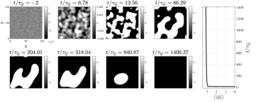
Figure 2: Snapshots of the density of order parameter at various time for periodic boundary conditions. (a) Time evolution of the domain walls without any topologically protected configurations. The white and black domains represent the positive and negative order parameters, while the interfaces are the domain walls; (b) The corresponding time evolution of the average absolute values of the order parameter in panel (a); (c) Snapshots of the evolution of topologically protected domain walls with $(w_{x}=0,w_{y}=1)$; (d) Snapshots of the evolution of the topologically protected domain walls with $(w_{x}=1,w_{y}=1)$.

III.2 Domain walls in two dimensions

Periodic Boundary Conditions: We first investigate the formation of domain walls in the two spatial dimensions with periodic boundary conditions, thus the topology of the background geometry is like a two dimensional torus as indicated in Fig.1(b). Numerically, we Fourier decompose the two spatial lengths to $10^{3}$ grids. We use the symbol $(w_{x},w_{y})$ to describe the windings that the domain wall may surround the periodic space in the $x$ and $y$ directions. We need to stress that since we are working with the periodic boundary conditions, the domain walls always appear in pairs [8, 9], i.e., domain wall and anti-domain wall. Here, $(w_{x},w_{y})$ just counts the winding number of the domain walls.

In the Fig.2(a) we show various time snapshots of the densities of the order parameter, ranging from the initial time $t/\tau_{Q}=-2$ to the final equilibrium state $t/\tau_{Q}=1406.37$. In this plot, white colors represent positive order parameter while black colors represent negative order parameters. We can vividly see how the order parameter evolves from random noise, to mosaic patterns (at $t/\tau_{Q}=6.78$ and $t/\tau_{Q}=13.56$), and then the coarsening dynamics render the domain walls (interfaces separating black and white areas) to bend and shrink (after $t/\tau_{Q}=86.29$). Finally the domain walls disappear and leave the whole negative order parameters in the space. Interestingly, we see that the evolution of the domain walls are in agreement with our speculations, from which the interfaces will bend and shrink according the mean curvatures at that point. Finally the uneven interface (at $t/\tau_{Q}=204.01$) will gradually shrink and become much more even (at $t/\tau_{Q}=940.87$). Since there is no obstacle in Fig.2(a) to prevent the interface to shrink, it will finally disappear and leave the whole negative order parameters there, i.e., there is no domain walls in the space. The numerical results from Fig.2(a) are totally in agreement with our speculations about the evolutions of domain walls with trivial topology and the sketches in Fig.1(c). From our notations, the final configuration of the domain wall is $(w_{x}=0,w_{y}=0)$. This configuration has the lowest free energy, thus is thermodynamically stable.

Fig.2(b) exhibits the evolution of the average of the absolute values of the order parameter. It will start with very tiny order parameters for a while and then ramp quickly to a plateau. It should be noted that during the course of the plateau the system is still evolving although very slowly. The coarsening dynamics in this stage will gradually shrink the domain walls, thus the values of $\langle|\phi|\rangle$ will gradually grow. Until the final time of vanishing domain walls, it will arrive at $\langle|\phi|\rangle\approx\sqrt{\epsilon_{f}}=\sqrt{10}$.

However, there are possibilities that the domain walls may wind around the torus and thus it cannot disappear due to the topological obstacles, as Fig.2(c) and Fig.2(d) show. For convenience, we only show five snapshots of the time evolution (from left to right) of the order parameter. From Fig.2(c) we see that during the coarsening dynamics the domain walls will shrink, and topologically trivial domain walls will finally disappear just as in Fig.2(a). However, it is interesting to see that at the final stage, there exists nontrivial configuration of the domain wall for $(w_{x}=0,w_{y}=1)$, i.e, the final state of the order parameter will have interface along only one of the circles of the torus, which is similar to the green loop in Fig.1(b). The final state of the domain wall in this case should be straight lines, otherwise they will move according to the curvatures. This is exactly what we saw from Fig.2(c). This straight line cannot break, otherwise there is no interface to separate the antiphase order parameters. From numerics we indeed found that this configurations of straight domain walls will exist permanently, meaning that they are dynamically stable. But from thermodynamics this configuration is an excited state rather than ground state. Since there is gradient energy existing in the domain walls, which have higher free energies than vanishing domain walls shown in Fig.2(a). Therefore, from thermodynamics this configuration is metastable. Thus, we have numerically demonstrated a topologically protected metastable state, which is in fact persistently stable.

Remarkably, it is still possible that there exists topologically protected state having higher free energies than that in Fig.2(c). In Fig.2(d) we show the domain wall structure with configurations $(w_{x}=1,w_{y}=1)$, which winds along $x$ and $y$-directions once respectively. This configuration corresponds to the red curve in Fig.1(b). The system now is a higher excited state than those in Fig.2(c) since the length of interfaces is longer than those in Fig.2(c). Because of the periodic boundary conditions and the identical lengths of $x$ and $y$-directions, the interfaces need to have an angle of $\pi/4$ against the $x$-direction. This is exactly the case in the Fig.2(d).

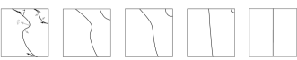
Figure 3: Snapshots of the evolution of the order parameter with Neumann boundary conditions. (a) Sketchy picture of the evolution of the domain walls. Black arrows represent the force acting at the boundary points while the gray arrows indicate the velocity vectors. The domain wall connecting the opposite boundaries will finally become straight and stay for ever. However, the domain wall in the corner (connecting the adjacent boundaries) will shrink and finally disappear; (b) Numerical results demonstrating the topologically protected domain walls having configuration $(w_{x}=0,w_{y}=1)$ with Neumann boundary conditions.

Neumann Boundary Conditions: At first sight, people may think that with Neumann boundary conditions the background geometry is trivial since it is not like the tours having topological obstacles there. However, as we shall see we can still have the chance to realize the topologically protected domain walls with Neumann boundary conditions. In Fig.3(a) we illustrate why there can still be topologically nontrivial domain walls with Neumann boundary conditions. The interface has surface tension, therefore, the force (black arrows) acting at the boundary points are pointing along the tangent direction of the interface. Due to the combination of the force at the boundary points and the velocity driven by the curvature, the interface which connects the opposite sides of the boundary will arrange itself and finally become a straight line perpendicular to the boundaries. This straight line can exist forever in time, meaning that it is dynamically stable. It should be noted that with Neumann boundary conditions the configurations of the domain walls are distinct from those with periodic boundary conditions. In particular, the domain wall does not need to appear in pairs with Neumann boundary conditions. We numerically demonstrate it in the Fig.3(b) which shows a domain wall with configuration $(w_{x}=0,w_{y}=1)$. From this we can deduce that even in the seemingly topologically trivial background geometry, we can still have the topologically protected metastable states. This result is consistent with our speculation that the domain walls are like the rubber bands, since in this case the rubber bands connecting the two moving points at the opposite sides will try to drag them in a straight line perpendicular to the boundaries. Alternatively, the final configuration of the fields is symmetric in $y$-direction, which resembles a cylinder if we wrap it along $y$-direction. Therefore, the interface is like a rubber band winding along the azimuthal direction of the cylinder, which is topologically protected due the hole of the cylinder.

However, the interfaces connecting the adjacent boundaries, for instance the curve in the corner in Fig.3(a), will shrink and finally disappear due the joint effect of the force at the boundary points and the velocities from the curvature. They are not the topologically protected domain walls. Fig.3(b) also shows the numerical evidences for this kind of domain walls.

III.3 Domain walls in three dimensions

In three dimensions we can still have the possibilities to realize the topologically protected metastable states. In three dimensions it is difficult to show the density of order parameter in the whole bulk, however, we can show the isosurface of the zero values of the order parameter. Since the zero value separates the positive and negative order parameter, we can regard the zero value surface as a representative of the domain wall. In Fig.4 we exhibit the snapshots of the evolution of the zero value surfaces in three dimensions with periodic boundary conditions. At the final time, we clearly see two topologically nontrivial flat surfaces indicating the topologically protected domain walls in three dimensions. One of the domain walls has the configuration $(w_{x}=1,w_{y}=1,w_{z}=0)$. Therefore, the topology of these domain walls are similar to those in Fig.2(c) although they are in different dimensions. The topology of domain walls similar to those in Fig.2(d) are hard to find in numerics. We believe that the probability is very low for this kind of skew surfaces. But Fig.4 already gave a strong evidence for the existence of a topologically protected metastable state in three dimensions.

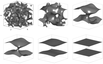
Figure 4: Snapshots of the evolution of the isosurface of zero values of the order parameter in three dimensions with periodic boundary conditions. The order of time is from (a) to (f).

IV Conclusions and Discussions

We speculated that the structures of the domain walls in the TDGL model at the final equilibrium state can have nontrivial topologies even though they are metastable states from the aspects of thermodynamics. As far as we know, this was the first time to realize the explicit forms of the topologically protected metastable states in classical dynamics. Our speculations mainly relied on the Allen-Cahn’s assertion that the velocity of domain wall was proportional to the mean curvature at that point. Therefore, the domain walls behaved as rubber bands which could bend, evolve and finally tightly wind around the background geometry in a nontrivial way. We numerically demonstrated our conjecture in two and three dimensions by using periodic and Neumann boundary conditions respectively.

In our model, we turned off the temperature of the system. However, temperature is not important to our conclusions. In fact we already checked that turning on the temperature by adding the Langevin noise term in the right side of Eq.(3), this model can still have the topologically protected metastable states, indicating that the existence of topologically protected metastable state has nothing to do with the temperature. As we have discussed, this metastable states protected by topology may potentially have practical use in the computer and information technology industry, such as the storage media since it has stable configurations of positive and negative order parameters.

References

- Zeng et al. [2019] B. Zeng, X. Chen, D.-L. Zhou, and X.-G. Wen, Quantum information meets quantum matter: From quantum entanglement to topological phases of many-body systems (Springer, 2019).
- Kopnin [2001] N. B. Kopnin, The Time-dependent Ginzburg-Landau Theory, in Theory of Nonequilibrium Superconductivity (Oxford University Press, 2001).
- Bray [2002] A. J. Bray, Theory of phase-ordering kinetics, Advances in Physics 51, 481 (2002).
- Hohenberg and Halperin [1977] P. C. Hohenberg and B. I. Halperin, Theory of dynamic critical phenomena, Reviews of Modern Physics 49, 435 (1977).
- Allen and Cahn [1979] S. M. Allen and J. W. Cahn, A microscopic theory for antiphase boundary motion and its application to antiphase domain coarsening, Acta metallurgica 27, 1085 (1979).
- Weinberg [1992] E. J. Weinberg, Classical solutions in quantum field theories, Annual Review of Nuclear and Particle Science 42, 177 (1992).
- Note [1] We need to stress that this interface cannot break during the evolutions, otherwise it cannot separates the antiphase order parameters.
- Del Campo [2018] A. Del Campo, Universal statistics of topological defects formed in a quantum phase transition, Physical Review Letters 121, 200601 (2018).
- del Campo et al. [2021] A. del Campo, F. J. Gómez-Ruiz, Z.-H. Li, C.-Y. Xia, H.-B. Zeng, and H.-Q. Zhang, Universal statistics of vortices in a newborn holographic superconductor: beyond the kibble-zurek mechanism, Journal of High Energy Physics 2021, 1 (2021).