From Authority-Respect to Grassroots-Dissent: Degree-Weighted Social Learning and Convergence Speed

Opinions are influenced by neighbors, with varying degrees of emphasis based on their connections. Some may value more connected neighbors’ views due to authority respect, while others might lean towards grassroots perspectives. The emergence of ChatGPT could signify a new “opinion leader” whose views people put a lot of weight on. This study introduces a degree-weighted DeGroot learning model to examine the effects of such belief updates on learning outcomes, especially the speed of belief convergence. We find that greater respect for authority doesn’t guarantee faster convergence. The influence of authority respect is non-monotonic. The convergence speed, influenced by increased authority-respect or grassroots dissent, hinges on the unity of elite and grassroots factions. This research sheds light on the growing skepticism towards public figures and the ensuing dissonance in public debate.

Introduction

In the interconnected web of social networks, people’s beliefs and opinions are intrinsically shaped by those around them. Not all voices carry the same weight: mainstream media, celebrities, and traditional authorities have historically held sway  (?). Yet, the shifting sands of public trust, particularly post-COVID, hint at an evolving dynamic where traditional experts face increasing skepticism.The digital age ushers in another layer of complexity with tools like ChatGPT, which blend the realms of technological advancement with societal influence, potentially ushering in a new echelon of opinion leaders  (?).

As beliefs evolve, the credence given to others’ views is often tied to their perceived influence and connectivity within their social network  (?). This phenomenon raises crucial questions: How does this weighting impact collective learning outcomes? Do beliefs converge faster when individuals respect authority more or when there is a prevalent grassroots dissent? These questions are especially pertinent given the growing skepticism towards public figures and in a world where authority and grassroots voices clash  (?).

To navigate this intricate terrain, we introduce a degree-weighted DeGroot learning model  (?). In this model, agents iteratively update their beliefs based on a weighted average of their neighbors’ current views, in which the weight depends on the neighbors’ social prominence  (?). Our novel approach allows the weight assigned to a neighbor’s view to be influenced by their number of connections, or, degree. A higher weight based on degree denotes “authority respect,” while a diminishing weight embodies “grassroots dissent”  (?). We endeavor to dissect the repercussions of this degree-dependence, especially its impact on the pace of belief convergence.

Our findings reveal an intriguing pattern: a heightened deference to authority does not invariably lead to quicker consensus. The speed at which beliefs converge, whether influenced by authority reverence or grassroots dissent, pivots on the unity within elite and grassroots factions  (?). Specifically, in scenarios with a singular elite and a singular grassroots group, amplifying either authority-respect or grassroots dissent can accelerate convergence (Figure 1). However, in settings with multiple elite or grassroots factions, increased deference to either can decelerate convergence (Figures 2 and 3). These outcomes offer a fresh lens to interpret the existing cacophony in public discourse.

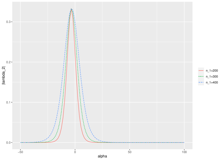
Figure 1: Graph of convergence speed versus the extent of degree-dependence when people update their beliefs. This graph shows that when there is one elite group and one grassroots group, either increasing authority respect (by increasing $\alpha$ from a threshold to $\infty$) or enhancing grassroots dissent (by decreasing $\alpha$ from a threshold to $-\infty$) can speed up convergence. The magnitude of the second largest eigenvalue of the learning matrix $\mathbf{T}^{*}$, denoted by $|\lambda_{2}(\mathbf{T}^{*})|$, is inversely related to the speed of convergence. The parameter $\alpha$ measures the degree-dependence of belief updating; a larger $\alpha$ indicates a greater influence of an individual’s degree in the updating process. When $\alpha=0$, individuals weigh their neighbors’ opinions equally, regardless of their degrees. In the graph, the weighting function is defined as $\phi(\alpha,d)=d^{\alpha}$, where $d$ is the degree of an individual. The size of the first group, $n_{1}$, is set to $200$, $300$, and $400$, and the total population size $n$ is $1000$. The within-group linking probability $p$ is $0.4$, and the between-group linking probability $q$ is $0.2$.

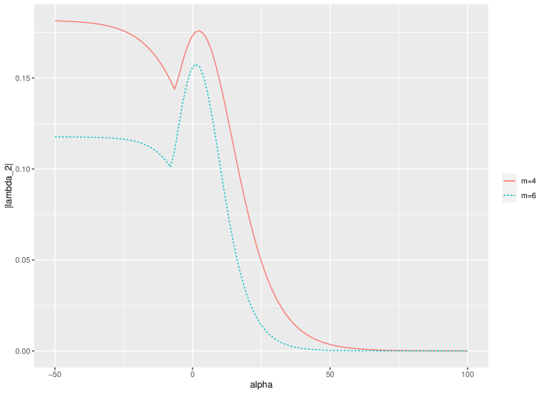
Figure 2: Graph of $|\lambda_{2}(\mathbf{T}^{*})|$ versus $\alpha$, with $\phi(\alpha,d)=d^{\alpha}$, $n_{1}=400$, $n=1000$, $p=0.5$, $q=0.3$, and $m=4,6$, representing the number of groups dividing the total population. This graph shows that when there is one elite group but multiple grassroots groups, increasing grassroots dissent (e.g., as $\alpha$ approaches $-\infty$) can lead to slower convergence. When $\alpha$ is negative and large in magnitude, the initial beliefs that lead to the slowest convergence are those in which grassroots groups hold different views from each other. Conversely, when $\alpha$ is positive and large, the initial beliefs that result in the slowest convergence are those where grassroots groups share the same views with each other, but these views differ from those of the elite group.

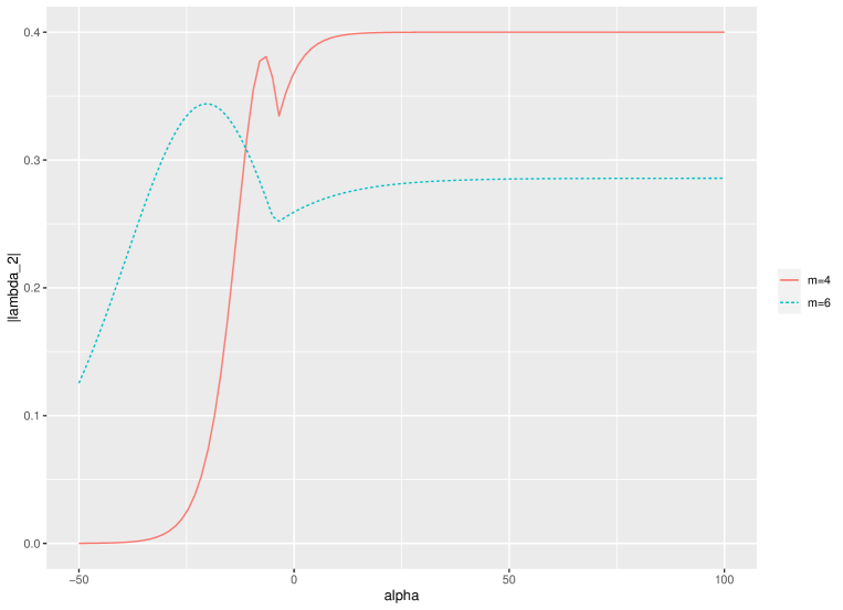
Figure 3: Graph of $|\lambda_{2}(\mathbf{T}^{*})|$ versus $\alpha$, with $\phi(\alpha,d)=d^{\,\alpha}$, $n_{1}=200$, $(m-1)n_{2}=1200$, $m=2,4,6$, $p=0.3$, $q=0.1$. This graph shows that when there is one grassroots group but multiple elite groups, increasing authority respect (e.g., when $\alpha\rightarrow\infty$) can lead to slower convergence. As a counterpoint to the scenario with one elite group and multiple grassroots groups, when $\alpha$ is positive and large, the initial beliefs that lead to the slowest convergence are those in which elite groups hold differing views from one another. In this case, the grassroots group acts as an information mediator between the conflicting elite groups. Thus, lowering the weight placed on elite groups (decreasing $\alpha$) results in a lower $\lambda_{2}$, signifying faster convergence. Conversely, when $\alpha$ is negative and large in magnitude, the initial beliefs that result in the slowest convergence are those where elite groups share identical views amongst themselves, yet these views differ from those of the grassroots group.

This refined model bridges the traditional DeGroot framework with contemporary societal nuances, placing emphasis on authority-respect and grassroots dissent. Existing literature in the DeGroot learning domain is categorized into three core themes: (1) whether beliefs convergence (as seen in  (?),  (?)); (2) whether beliefs converge to truth (e.g.,  (?)); and (3) how fast beliefs converge ( (?),  (?),  (?)). Our research offers fresh insights into the third theme, with a particular focus on the velocity of belief convergence. Delving deeper, while prior works have explored the role of network structures (such as  (?)’s study on homophily) and learning heuristics (e.g.,  (?)), our contribution stands as a pioneering examination of the influence of degree-weighted learning on convergence speed.

Results

To investigate the influence of degree-weighted learning heuristics on belief convergence rates, we structure our exposition through a series of methodical steps. Initially, we integrate a degree-weighted learning heuristic into the established DeGroot learning framework. Subsequently, we delineate the metric for convergence speed within this augmented model. In the penultimate phase, we employ the stochastic block model to introduce a variable degree of heterogeneity among the agents. Finally, we demonstrate how varying degrees of deference to authority can significantly alter the rate at which convergence is achieved.

Basic network. Consider a network consisting of $n$ vertices, which is represented by an undirected graph comprising vertices and edges. The associated $n\times n$ adjacency matrix $\mathbf{A}$ is defined as follows: $A_{ij}=A_{ji}=1$ if there is an edge between vertices $i$ and $j$; otherwise, $A_{ij}=A_{ji}=0$. The structure of the network is completely characterized by the adjacency matrix $\mathbf{A}$.

DeGroot learning model. In the classical DeGroot learning model  (?), an agent’s belief—such as the probability of global warming or the safety of a COVID vaccine—is formed through a simple linear aggregation of the neighboring agents’ beliefs from the previous period. Specifically, the belief vector $\mathbf{b}(t)$ at a discrete time $t$, where $t$ belongs to the set of natural numbers $\mathbb{N}=\{0,1,2,\ldots\}$, is defined as follows:

$$\mathbf{b}(t)=\mathbf{T}^{t}\mathbf{b}_{0}\,,$$

where $\mathbf{b}_{0}\in\mathbb{R}^{n}$ with $\|\mathbf{b}_{0}\|_{2}=1$ is the initial belief vector, and $\mathbf{T}$, the learning matrix, is an $n\times n$ row-stochastic matrix. In this matrix, each element $T_{ij}$ represents the weight that vertex $i$ assigns to the belief of vertex $j$.

The abstract learning matrix $\mathbf{T}$ encapsulates two types of information: the structure of a network, which is encoded within the adjacency matrix $\mathbf{A}$, and the learning heuristic. For example, when agents assign equal weight to their neighbors, as posited by  (?), the matrix $\mathbf{T}$ is defined by the relation $T_{ij}=A_{ij}/d_{i}(\mathbf{A})$, where $d_{i}(\mathbf{A})=\sum_{j}A_{ij}$ represents the degree of vertex $i$—that is, the number of connections or friends agent $i$ possesses. This formulation presumes that each vertex allocates equal importance to all of its neighbors, thus allowing the authors to concentrate on examining the influence of network structure on the rate of learning.

Degree-weighted learning matrix. The impetus for our work is an observable pattern within real-world updating processes: individuals often weight their neighbors’ opinions according to the neighbor’s popularity, or their degree, to use network terminology. Celebrities, for example, attract considerable attention, and historically, in many societies, there has been an unwavering respect for the opinions of authority figures. Conversely, due to technological advancements, such as the advent of social media, the opinions of the general populace have become more accessible than ever before. This observation suggests a learning heuristic wherein the updating process is contingent upon degree.

To encapsulate the aforementioned dynamics, we introduce a new degree-weighted learning matrix $\mathbf{T}$, defined as follows:

$$T_{ij}=\frac{A_{ij}\phi(\alpha,d_{j}(\mathbf{A}))}{\sum\limits_{k}A_{ik}\phi(\alpha,d_{k}(\mathbf{A}))}\,,$$ (1)

where $\phi:\mathbb{R}^{2}\to\mathbb{R}$ is a function that modulates the influence of the degree of vertices, and the parameter $\alpha\in\mathbb{R}$ introduces additional flexibility in analyzing variations in beliefs and convergence rates as the matrix $\mathbf{T}$ changes. With all other factors held constant, the alteration in $\mathbf{T}$ within our framework is signified by a shift in $\alpha$. The formulation in Eq. (1) is designed to capture the heterogeneity of vertices in accordance with their degrees, and the function $\phi$ provides the necessary generality for this model.

Under the premise that vertices with higher degrees, such as celebrities, experts, or opinion leaders, are deemed more influential, we naturally posit that the function $\phi$ is monotonically increasing with the degree $d$. Conversely, it is also pertinent to explore scenarios where higher degree vertices are assigned lower weights, reflecting a dynamic similar to grassroots dissent, where, facilitated by technological advancements, the opinions of the broader community have become more readily available. To accommodate the analysis of both dynamics, we define $\phi$ to be increasing in $d$ for $\alpha\in(0,\infty)$ and decreasing for $\alpha\in(-\infty,0)$, with $\phi$ set to a constant value of 1 at $\alpha=0$, serving as a benchmark. Throughout this paper, we employ $\phi(\alpha,d)=d^{\alpha}$ as the canonical form. When $\alpha=0$, this yields the uniform weighting scenario as in  (?); we term the case with $\alpha>0$ as “authority-respect” and the $\alpha<0$ scenario as “grassroots-dissent.”

Stochastic block model. In exploring the effects of degree dependence on learning outcomes, we require a degree-heterogeneous social network model. To achieve this goal, we employ the stochastic block model ( (?),  (?),  (?)), a random graph model that has been rigorously examined and is prevalently utilized in network analysis literature, exemplified by  (?),  (?),  (?), and  (?).

Specifically, suppose there are $m$ groups of vertices. Let $\mathbf{P}$ be an $m\times m$ symmetric matrix. Then, for $i\leq j$ (i.e., the upper triangular part of $\mathbf{A}$), let $A_{ij}$ be independent Bernoulli random variables, with $A_{ij}=\text{Bernoulli}(P_{kl})$ if vertex $i$ belongs to group $k$ and vertex $j$ belongs to group $l$. For $i>j$, set $A_{ij}=A_{ji}$. Let $\mathbf{n}=(n_{1},\ldots,n_{m})$, where each $n_{k}$ is the number of vertices in group $k$, for $k\in\{1,\ldots,m\}$. For clarity, we denote the random matrix generated by the stochastic block model as $\mathbf{A}(\mathbf{P},\mathbf{n})$.

Elite-Grassroots model. We introduce a case referred to as the Elite-Grassroots model, consisting of $n$ agents distributed into $m\geq 2$ groups, with each group comprising $n_{i}$ agents for $i\in\{1,\cdots,m\}$. The linking probability matrix $\mathbf{P}$ is structured as follows:

$${}\mathbf{P}=\begin{bmatrix}p&q&\ldots&q\\ q&p&\ldots&q\\ \vdots&\vdots&\ddots&\vdots\\ q&q&\ldots&p\end{bmatrix}\,,$$ (2)

where $p$ denotes the within-group linking probability, and $q$ the between-group linking probability. The ratio of $p$ to $q$ serves as a measure of homophily; a greater $p$ compared to $q$ indicates a more homophilous network. We make the following assumption regarding group sizes:

Assumption 1 (Two Group Sizes).

$$n_{1}\neq n_{2}=\ldots=n_{m}.$$ (3)

Convergence speed. Firstly, we define convergence speed as used in our paper.

Definition 1 (Convergence Speed).

Denote $\mathbf{T}^{\infty}=\lim_{t\rightarrow\infty}\mathbf{T}^{t}$. At time $t$, the convergence speed is quantified by the expression

$$\max\limits_{\|\mathbf{b}_{0}\|_{2}=1}\|(\mathbf{T}^{t}-\mathbf{T}^{\infty})\mathbf{b}_{0}\|_{2},$$ (4)

where $\|\cdot\|_{2}$ denotes the Euclidean norm. This expression measures the maximum distance between the belief at time $t$ and the limiting belief, for all possible initial beliefs. A larger distance implies a slower convergence speed.

The worst-case initial belief vector provides the most representative measure of the network’s consensus-reaching capability. Conversely, specific cases like $\mathbf{b}_{0}=(1/\sqrt{n},\ldots,1/\sqrt{n})^{\top}$, indicating immediate convergence, are less informative for our analysis.

Mathematical literature indicates that the magnitude of the second largest eigenvalue of the learning matrix $\mathbf{T}$ critically influences convergence speed (see  (?) for instance). Our first result confirms this relationship in our context.

Lemma 1 (Convergence Speed Inversely Related to $|\lambda_{2}|$).

Given $\mathbf{T}^{\infty}=\lim_{t\rightarrow\infty}\mathbf{T}^{t}$, at time $t$,

$$\max\limits_{\|\mathbf{b}_{0}\|_{2}=1}\|(\mathbf{T}^{t}-\mathbf{T}^{\infty})\mathbf{b}_{0}\|_{2}=|\lambda_{2}(\mathbf{T})|^{t}\,,$$ (5)

where $\lambda_{2}(\mathbf{T})$ is the second largest eigenvalue in magnitude of $\mathbf{T}$ and $\|\cdot\|_{2}$ is the Euclidean norm.

Here, the term $\max_{\|\mathbf{b}_{0}\|_{2}=1}\|(\mathbf{T}^{t}-\mathbf{T}^{\infty})\mathbf{b}_{0}\|_{2}$ describes the distance between current beliefs and the ultimate consensus as defined in Definition 1. With the largest eigenvalue of a row-stochastic matrix being 1, the expression on the right side of equation (5) diminishes to zero as $t$ increases, and thus $|\lambda_{2}(\mathbf{T})|$ primarily determines the convergence speed.

Results for “Expectation”–Replacing $\mathbf{A}$ with $\mathbb{E}[\mathbf{A}]$. With the foundational concepts established, our task is to determine the second largest eigenvalue (in magnitude) of $\mathbf{T}$. Considering the stochastic block model, $\mathbf{T}$ is inherently a random variable. Here, we present our results concerning the expectations of $\mathbf{T}$. In Section Materials and Methods, we complete the analysis by demonstrating that the difference between a random network and its expected value becomes negligibly small for a sufficiently large $n$.

Recall that $\mathbf{A}(\mathbf{P},\mathbf{n})$ denotes the random matrix generated by the stochastic block model. Now, define $\mathbf{R}=\mathbb{E}[\mathbf{A}(\mathbf{P},\mathbf{n})]$, where $\mathbf{R}$ is the expected adjacency matrix, with $R_{ij}=P_{kl}$ when vertex $i$ is in group $k$ and vertex $j$ is in group $l$. Let $\mathbf{T}^{*}$ denote the linear updating mechanism, which we define using $\mathbf{R}$ as follows:

$$T^{*}_{ij}=\frac{R_{ij}\,\phi(\alpha,d_{j}(\mathbf{R}))}{\sum\limits_{j}R_{ij}\,\phi(\alpha,d_{j}(\mathbf{R}))}\,,$$ (6)

where we define the expected degree $d_{i}(\mathbf{R})$ as follows: $d_{i}(\mathbf{R})=\mathbb{E}[d_{i}(\mathbf{A})]=\sum_{j}R_{ij}$ for $i=1,\ldots,n$. In the definition of $\mathbf{T}^{*}$, note that we replace all instances of $\mathbf{A}$ with $\mathbf{R}$ in the expression of $\mathbf{T}$ in (1).

We first summarize below that under our model specifications, agents fall into only two categories, distinguished by their expected degrees (i.e., the expected number of connections).

Lemma 2 (Elite and Grassroots).

Let $d_{i}^{*}$ denote the expected degree of group $i\in\{1,\ldots,m\}$. The expected degree of vertex $i$, denoted by $d_{i}(\mathbf{R})$, is $d_{1}^{*}$ if vertex $i$ belongs to group 1 and $d_{i}(\mathbf{R})=d_{2}^{*}$ for all other vertices, where $d_{1}^{*}=n_{1}p+(m-1)n_{2}q$ and $d_{2}^{*}=n_{1}q+n_{2}p+(m-2)n_{2}q$.

We term the group with the larger expected degree the elite, and the group with the smaller expected degree the grassroots. We are now ready to fully characterize the second largest eigenvalue and the impact of $\alpha$ on it.

Theorem 1 (Impact of Degree-Dependence $\alpha$).

We find that $|\lambda_{2}(\mathbf{T}^{*})|$ is monotonically decreasing in $\alpha$ for $\alpha\in\mathcal{D}_{\alpha}$ and monotonically increasing for $\alpha\notin\mathcal{D}_{\alpha}$, where $\mathcal{D}_{\alpha}$ is defined by

$$\mathcal{D}_{\alpha}=\begin{cases}\bigg{[}g^{-1}\left(\frac{n_{1}}{n_{2}}\right),\infty\bigg{)}.,&\mbox{if }m=2\\ (-\infty,g^{-1}(n_{1}/n_{2})]\cup\bigg{[}g^{-1}\left(\frac{n_{1}}{n_{2}}\left(\frac{p}{(m-1)(p+(m-2)q)}\right)^{1/2}\right),\infty\bigg{)},&\mbox{if }m\geq 3,d_{1}^{*}>d_{2}^{*}\\ \bigg{(}g^{-1}\left(\frac{n_{1}}{n_{2}}\left(\frac{p}{(m-1)(p+(m-2)q)}\right)^{1/2}\right),g^{-1}(n_{1}/n_{2})\bigg{]},&\mbox{if }m\geq 3,d_{1}^{*}<d_{2}^{*}.\end{cases}$$ (7)

In other words, when there is only one elite group and one grassroots group (Case 1), an increase in $\alpha$ beyond $g^{-1}(\frac{n_{1}}{n_{2}})$ as well as a decrease in $\alpha$ below this threshold can both lead to faster belief convergence. In the scenario with one elite group and multiple grassroots groups (Case 2), a higher $\alpha$ accelerates belief convergence, whereas a lower $\alpha$ decelerates it. Conversely, with one grassroots group and multiple elite groups (Case 3), a lower $\alpha$ facilitates faster convergence, while a higher $\alpha$ results in slower convergence. Figure 4 illustrates the impact of $\alpha$ for Cases 1 and 2 under different parameter specifications, and Figure 5 presents Cases 1 and 3.

Discussion

Understanding Regime Changes. Our results demonstrate that neither amplifying authority-respect nor grassroots dissent guarantees faster convergence. The intuition behind this can be best understood by examining the regime changes in each case. With only one elite and one grassroots group (Case 1), agents relying heavily on grassroots opinions ($\alpha$ approaching $-\infty$) result in the grassroots group becoming dominant; similarly, with utmost trust in authorities ($\alpha$ approaching $+\infty$), the elite group prevails. As $\alpha$ shifts from $-\infty$ to $g^{-1}(\frac{n_{1}}{n_{2}})$, society transitions from one dominant viewpoint to two—one from the elite and the other from the grassroots—slowing belief convergence as we increase $\alpha$ in this region. Further increases in $\alpha$ lead society back to a single dominant viewpoint, accelerating belief convergence.

Whereas when there is one elite group and multiple grassroots groups, increasing grassroots dissent (i.e., when $\alpha$ decreases from $g^{-1}(\frac{n_{1}}{n_{2}})$ to $-\infty$) leads to the slowest convergence with the worst initial beliefs, where different grassroots groups hold different opinions from one another. In other words, the views are not unified within the grassroots groups. Conversely, as we increase authority respect (i.e., when $\alpha$ increases from $g^{-1}(\frac{n_{1}}{n_{2}})$ to $+\infty$), the worst initial beliefs converge to a scenario in which the elite group has one view, and all grassroots groups share a different, but collective view. This brings us back to Case 1, where there is only one elite group and one grassroots group. Lastly, understanding the dynamics behind Case 2 makes it easier to grasp Case 3, where there is one grassroots group and multiple elite groups, which is essentially the reverse of Case 2.

Takeaway. Our study sheds light on the influence of skepticism towards experts and the discord in public discourse. In society’s complex discourse, our views are shaped by various influences, from authorities to grassroots movements and opinion leaders. The weight we give to each voice can significantly affect the persistence of societal disagreements. The key takeaway is that a pronounced respect for authority does not uniformly speed up consensus. The rate of belief convergence, influenced by deference to authority or grassroots dissent, depends on the unity within the elite and grassroots factions.

Limitations and Future Work. Our study employs an agent’s network of connections, or “degree,” as a surrogate for attributes like influence, fame, and popularity. This degree-dependent method in our updating matrix captures essential aspects of social learning. However, there are potential alternative dimensions to consider. For instance, during information updates, the weighting matrix might be based on the precision of an agent’s signal rather than their neighbors’ degree. While this presents a compelling avenue of exploration, a thorough analysis of such dimensions is reserved for future research.

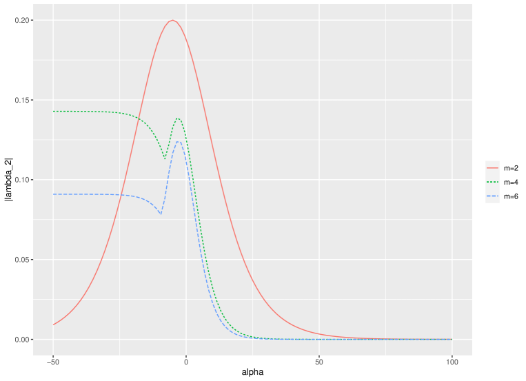
Figure 4: Graph of $|\lambda_{2}(\mathbf{T}^{*})|$ vs. $\alpha$, with $\phi(\alpha,d)=d^{\,\alpha}$, $n_{1}=500$, $n_{2}=300$, $p=0.3$, $q=0.2$ and $m=2,4,6$. This graph shows that when there is one elite group but multiple grassroots groups, increasing grassroots dissent (e.g., when $\alpha\rightarrow-\infty$) can cause slower convergence.

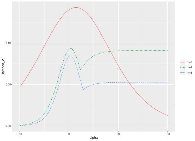
Figure 5: Graph of $|\lambda_{2}(\mathbf{T}^{*})|$ vs. $\alpha$, with $\phi(\alpha,d)=d^{\,\alpha}$, $n_{1}=800$, $(m-1)n_{2}=600$, $p=0.3$, $q=0.4$ and $m=2,4,6$. This graph shows that when there is one grassroots group but multiple elite groups, increasing authority respect (e.g., when $\alpha\rightarrow\infty$) can lead to slower convergence.

Materials and Methods

We showed our results using an example of the degree-dependent function $\phi(d)=d^{\alpha}.$ All results hold for general $\phi$ as long as it satisfies the following properties:

Property 1.

$\phi(\alpha,d)\in\mathcal{C}^{2}(\mathbb{R}\times[0,\infty))$ is nonnegative and $\phi(0,d)\equiv 1$ for all $d\in[0,\infty)$. In addition, $\phi$ is monotonically increasing in $\alpha$ for $\alpha\in\mathbb{R}$, monotonically increasing in $d$ for $\alpha\in(0,\infty)$ and monotonically decreasing in $d$ for $\alpha\in(-\infty,0)$.

Property 2.

For any two degrees $d_{1}>d_{2}$, the ratio $\phi(\alpha,d_{2})/\phi(\alpha,d_{1})$ is strictly decreasing in $\alpha$:

$$\frac{d}{d\alpha}\left(\frac{\phi(\alpha,d_{2})}{\phi(\alpha,d_{1})}\right)<0\,.$$ (8)

In addition, $\lim\limits_{\alpha\rightarrow\infty}\frac{\phi(\alpha,d_{2})}{\phi(\alpha,d_{1})}=\lim\limits_{\alpha\rightarrow-\infty}\frac{\phi(\alpha,d_{1})}{\phi(\alpha,d_{2})}=0$.

Property 3.

$\phi$ satisfies

$$\limsup_{d\rightarrow\infty}\frac{\partial\phi(\alpha,d)/\partial d}{\phi(\alpha,d)/d}<\infty\,,$$ (9)

and

$$\limsup_{d\rightarrow\infty}\frac{\,\partial^{2}\phi(\alpha,d)/\partial d^{2}}{(\partial\phi(\alpha,d)/\partial d)/d}<\infty\,.$$ (10)

Properties 1 and 2 are the very basic requirements for $\phi$ in order for our discussion to be meaningful. Property 3 consists of two technical conditions needed for the concentration result that we derive later in Lemma 3 for random networks. Roughly speaking, Property 3 says that we do not want a tiny change in the degree $d$ to cause a huge increase in the $\phi$.

Fully characterizing $\lambda_{2}$

Theorem 1 relies on the following result which fully characterizes the second largest eigenvalue in magnitude of learning matrix $\mathbf{T}^{*}$.

Proposition 1 ($\lambda_{2}$ in Elite-Grassroots Model).

Recall that $d_{1}^{*}=n_{1}p+(m-1)n_{2}q$ and $d_{2}^{*}=n_{1}q+n_{2}p+(m-2)n_{2}q$ be the expected degrees and let $g:\mathbb{R}\rightarrow\mathbb{R}$ be the function:

$$g(\alpha)=\frac{\phi(\alpha,d_{2}^{*})}{\phi(\alpha,d_{1}^{*})},$$ (11)

where $\phi$ satisfy Properties 1 - 3. Then under assumptions of linking probabilities and group sizes in (2) and (3) we have:

When $m=2$ (Case (1)), the second largest eigenvalue (in magnitude) is:

$$|\lambda_{2}(\mathbf{T}^{*})| =\left|\frac{n_{1}p\,\phi(\alpha,d_{1}^{*})}{n_{1}p\,\phi(\alpha,d_{1}^{*})+n_{2}q\,\phi(\alpha,d_{2}^{*})}-\frac{n_{1}q\,\phi(\alpha,d_{1}^{*})}{n_{1}q\,\phi(\alpha,d_{1}^{*})+n_{2}p\phi(\alpha,d_{2}^{*})}\right|\,$$ (12)

When $m\geq 3$ and $d_{1}^{*}>d_{2}^{*}$ (Case (2)), we have:

$$|\lambda_{2}(\mathbf{T}^{*})|=\begin{cases}|\frac{n_{1}p\,\phi(\alpha,d_{1}^{*})}{n_{1}p\,\phi(\alpha,d_{1}^{*})+(m-1)n_{2}q\,\phi(\alpha,d_{2}^{*})}\\ \quad-\frac{n_{1}q\,\phi(\alpha,d_{1}^{*})}{n_{1}q\,\phi(\alpha,d_{1}^{*})+(n_{2}p+(m-2)n_{2}q)\phi(\alpha,d_{2}^{*})}|\,,\quad&\alpha\geq g^{-1}(n_{1}/n_{2})\\ \left|\frac{n_{2}(p-q)\,\phi(\alpha,d_{2}^{*})}{n_{1}q\,\phi(\alpha,d_{1}^{*})+(n_{2}p+(m-2)n_{2}q)\phi(\alpha,d_{2}^{*})}\right|\,,\quad&\alpha<g^{-1}(n_{1}/n_{2})\end{cases}$$ (13)

When $m\geq 3$ and $d_{1}^{*}<d_{2}^{*}$ (Case (3)), the second largest (in magnitude) eigenvalue is:

$$|\lambda_{2}(\mathbf{T}^{*})|=\begin{cases}|\frac{n_{1}p\,\phi(\alpha,d_{1}^{*})}{n_{1}p\,\phi(\alpha,d_{1}^{*})+(m-1)n_{2}q\,\phi(\alpha,d_{2}^{*})}\\ \quad-\frac{n_{1}q\,\phi(\alpha,d_{1}^{*})}{n_{1}q\,\phi(\alpha,d_{1}^{*})+(n_{2}p+(m-2)n_{2}q)\phi(\alpha,d_{2}^{*})}|\,,\quad&\alpha\leq g^{-1}(n_{1}/n_{2})\\ \left|\frac{n_{2}(p-q)\,\phi(\alpha,d_{2}^{*})}{n_{1}q\,\phi(\alpha,d_{1}^{*})+(n_{2}p+(m-2)n_{2}q)\phi(\alpha,d_{2}^{*})}\right|\,,\quad&\alpha>g^{-1}(n_{1}/n_{2})\end{cases}$$ (14)

Worst initial beliefs

It can be shown that the second eigenvector of $\mathbf{T^{*}}$ takes the following form:

$$\mathbf{v}_{2}=(\underbrace{v_{21},\ldots,v_{21}}_{n_{1}},\underbrace{v_{22},\ldots,v_{22}}_{n_{2}},\ldots,\underbrace{v_{2m},\ldots,v_{2m}}_{n_{2}})^{\top}.$$

Note here that since agents within the same group are identical ex ante, their beliefs quickly converge after one period of updating. As a result, in expectation, agents in the same group hold identical views. Only beliefs across groups could differ.

Then we have for case 1, i.e., $m=2$:

$$v_{21}=-\frac{b}{en_{2}+n_{1}b^{2}/e},\ v_{22}=\frac{1}{n_{2}+n_{1}b^{2}/e^{2}}\,.$$

In other words, when we have only two groups of agents, for each $\alpha$, the initial beliefs that lead to slowest convergence is the one that elite group holds a different view than the grassroots group.

For case 2, when $m\geq 3$ and there is one elite group and multiple grassroots groups: if $\alpha>g^{-1}(\frac{n_{1}}{n_{2}})$, the worst initial beliefs are that elite group agents share the same initial beliefs, and all the grassroots groups share the same beliefs. Whereas when $\alpha<g^{-1}(\frac{n_{1}}{n_{2}})$, the worst initial beliefs are that elite group agents share the same belief, but the grassroots groups hold different opinions from each other (i.e., grassroots groups $2$ to $m$ holds different initial views).

Moving to case 3 in which there is one grassroots group and multiple elite groups, if $\alpha>g^{-1}(\frac{n_{1}}{n_{2}})$, the worst initial beliefs are such that different elite groups hold different views, and grassroots agents hold the same view; and when $\alpha<g^{-1}(\frac{n_{1}}{n_{2}})$, the worst initial beliefs are such different elite groups holds the same view, but the view is different from grassroots view. More formally, the following proposition summarizes the above results about worst initial beliefs.

Proposition 2.

Denote the second eigenvector of $\mathbf{T^{*}}$ by

$$\mathbf{v}_{2}=(\underbrace{v_{21},\ldots,v_{21}}_{n_{1}},\underbrace{v_{22},\ldots,v_{22}}_{n_{2}},\ldots,\underbrace{v_{2m},\ldots,v_{2m}}_{n_{2}})^{\top}.$$

For $d_{1}^{*}>d_{2}^{*}$, when $\alpha>g^{-1}(\frac{n_{1}}{n_{2}})$, we have

$$v_{21}=-\frac{(m-1)b}{e(m-1)n_{2}+n_{1}(m-1)^{2}b^{2}/e},\ v_{22}=\ldots=v_{2m}=\frac{1}{(m-1)n_{2}+n_{1}(m-1)^{2}b^{2}/e^{2}}\,.$$

When $\alpha<g^{-1}(\frac{n_{1}}{n_{2}})$, let $\mathbf{v}^{\prime}=(\underbrace{v^{\prime}_{1},\ldots,v^{\prime}_{1}}_{n_{1}},\underbrace{v^{\prime}_{2},\ldots,v^{\prime}_{2}}_{n_{2}},\ldots,\underbrace{v^{\prime}_{m},\ldots,v^{\prime}_{m}}_{n_{2}})^{\top}$, where

$$v^{\prime}_{1}=-\frac{(m-1)b}{e(m-1)n_{2}+n_{1}(m-1)^{2}b^{2}/e},\ v^{\prime}_{2}=\ldots=v^{\prime}_{m}=\frac{1}{(m-1)n_{2}+n_{1}(m-1)^{2}b^{2}/e^{2}}\,.$$

then $(\mathbf{D}_{1,\mathbf{R}}\mathbf{D}_{2,\mathbf{R}})^{-1/2}\mathbf{v}_{2}$ is any vector orthogonal to $(\mathbf{D}_{1,\mathbf{R}}\mathbf{D}_{2,\mathbf{R}})^{1/2}\mathbf{v}^{\prime}$ and $(\mathbf{D}_{1,\mathbf{R}}\mathbf{D}_{2,\mathbf{R}})^{1/2}\mathbf{1}$, where $\mathbf{D}_{1,\mathbf{R}}$ and $\mathbf{D}_{2,\mathbf{R}}$ are diagonal matrices defined by:

$$(\mathbf{D}_{1,\mathbf{R}})_{ii}=\sum_{j}R_{ij}\,\phi(\alpha,d_{j}(\mathbf{R}))\,,$$

$$(\mathbf{D}_{2,\mathbf{R}})_{ii}=\phi(\alpha,d_{i}(\mathbf{R}))\,,$$

in which $\mathbf{T}^{*}=\mathbf{D}^{-1}_{1,\mathbf{R}}\mathbf{R}\mathbf{D}_{2,\mathbf{R}}\,,$ and $\mathbf{R}={\rm I}\kern-1.79993pt{\rm E}\mathbf{A}$.

When $\alpha=g^{-1}(\frac{n_{1}}{n_{2}})$, $(\mathbf{D}_{1,\mathbf{R}}\mathbf{D}_{2,\mathbf{R}})^{-1/2}\mathbf{v}_{2}$ is any vector orthogonal to $(\mathbf{D}_{1,\mathbf{R}}\mathbf{D}_{2,\mathbf{R}})^{1/2}\mathbf{1}$.

In contrast if $d_{1}^{*}<d_{2}^{*}$, when $\alpha<g^{-1}(\frac{n_{1}}{n_{2}})$, we have

$$v_{21}=-\frac{(m-1)b}{e(m-1)n_{2}+n_{1}(m-1)^{2}b^{2}/e},\ v_{22}=\ldots=v_{2m}=\frac{1}{(m-1)n_{2}+n_{1}(m-1)^{2}b^{2}/e^{2}}\,.$$

When $\alpha>g^{-1}(\frac{n_{1}}{n_{2}})$, then $(\mathbf{D}_{1,\mathbf{R}}\mathbf{D}_{2,\mathbf{R}})^{-1/2}\mathbf{v}_{2}$ is any vector orthogonal to $(\mathbf{D}_{1,\mathbf{R}}\mathbf{D}_{2,\mathbf{R}})^{1/2}\mathbf{v}^{\prime}$ and $(\mathbf{D}_{1,\mathbf{R}}\mathbf{D}_{2,\mathbf{R}})^{1/2}\mathbf{1}$.

When $\alpha=g^{-1}(\frac{n_{1}}{n_{2}})$, $(\mathbf{D}_{1,\mathbf{R}}\mathbf{D}_{2,\mathbf{R}})^{-1/2}\mathbf{v}_{2}$ is any vector orthogonal to $(\mathbf{D}_{1,\mathbf{R}}\mathbf{D}_{2,\mathbf{R}})^{1/2}\mathbf{1}$.

For $m=2$, the second eigenvector is

$$v_{21}=-\frac{b}{en_{2}+n_{1}b^{2}/e},\ v_{22}=\frac{1}{n_{2}+n_{1}b^{2}/e^{2}}\,.$$

Results for random learning matrix

Section 1 summarizes our findings about convergence speed in the case of “expectation.” To see the full picture, we need to show that the result for the random case is arbitrarily “close” to the “expectation” when $n$ is sufficiently large. To address this issue, we first make a few assumptions:

Assumption 2 (Density).

Let $\tau_{n}=\min\limits_{i}\frac{d_{i}(\bm{R})}{n}$, where $\mathbf{R}={\rm I}\kern-1.79993pt{\rm E}\mathbf{A}$. Assume that

$$\lim_{n\rightarrow\infty}\frac{\tau_{n}}{\sqrt{\frac{\log n}{n}}}=\infty\,.$$ (15)

Assumption 3 (No Vanishing Groups).

For all $k=1,\ldots,m$:

$$\liminf_{n}\frac{n_{k}}{n}>0\,.$$ (16)

Assumption 4 (Comparable Densities).

$$\limsup_{n}\frac{p_{n}}{q_{n}}<\infty\,.$$ (17)

We note first that with the minimum density assumed (Assumption 2), the network is connected with high probability. Restricting to this high probability event, the directed graph $\mathcal{G}(\mathbf{T})$ corresponding to the matrix $\mathbf{T}$ is strongly connected. In addition, $\mathbf{T}$ is aperiodic with high probability. With the known fact that strongly connectivity and aperiodicity together implies convergence (see  (?)), we see that the limit exists with high probability. We characterize what limit beliefs look like in the following proposition.

Proposition 3 (Consensus).

The limit $\mathbf{T}^{\infty}$ as $t\rightarrow\infty$ is given by:

$$\mathbf{T}^{\infty}=\begin{bmatrix}T_{1}&T_{2}&\ldots&T_{n}\\ T_{1}&T_{2}&\ldots&T_{n}\\ \vdots&\vdots&\ddots&\vdots\\ T_{1}&T_{2}&\ldots&T_{n}\end{bmatrix}\,,$$

where

$$T_{j}=\frac{\sum\limits_{i}A_{ij}\,\phi(\alpha,d_{j}(\mathbf{A}))\phi(\alpha,d_{i}(\mathbf{A}))}{\sum\limits_{i,j}A_{ij}\,\phi(\alpha,d_{j}(\mathbf{A}))\phi(\alpha,d_{i}(\mathbf{A}))}\,,$$

for $j=1,\ldots,n$. This means that the limiting beliefs $\mathbf{b}(\infty)=\mathbf{T}^{\infty}\mathbf{b}_{0}$ would shift towards the beliefs of high degree neighbors as $\alpha$ increases.

With Assumptions 2 - 4, we achieve our main technical Lemma:

Lemma 3.

Suppose $\mathbf{A}(\mathbf{P},\mathbf{n})$ is generated by the stochastic block model with $\mathbf{P}$ and $\mathbf{n}$. In addition, suppose Assumptions 2, 3, and 4 hold. Then, there exists a positive constant $\tilde{C}$, independent of $n$, such that for all $n>0$,

$$\operatorname{\mathbb{P}}\left\{|\lambda_{2}(\mathbf{T})-\lambda_{2}(\mathbf{T}^{*})|\geq\tilde{C}\frac{\sqrt{\log n}}{\tau_{n}\sqrt{n}}\right\}\leq\frac{16}{n^{2}}\,.$$

Note for this lemma, we do not require the structure assumed in elite-grassroots model (i.e., we do not need Assumption 1). By Lemma 3, we see that the error gets arbitrarily small when $n$ goes to infinity. The remaining part is that although the monotonicity in the case “expectation” does not happen in the case of random networks, we can still find out how much increase in $\alpha$ could give a decrease in the eigenvalue that exceeds the error created by randomness. Given an $\alpha_{0}$, suppose $\alpha$ rises from $\alpha_{0}$ to $\alpha_{1}$, then how large do $\alpha_{1}$ need to be to see an increase in the the convergence speed with high probability? We answer this question by applying Lemma 3 in the following theorem.

Theorem 2.

Given a constant $\alpha_{0}$. Let $\alpha_{1}$ be bounded away from $\infty$. If $\alpha_{0},\alpha_{1}\in\mathcal{D}_{\alpha}$ as defined in Theorem 1 and

$$\alpha_{1}-\alpha_{0}>\hat{C}\frac{\sqrt{\log n}}{\tau_{n}\sqrt{n}}\left[\frac{\partial\phi/\partial\alpha(\alpha_{1},d_{1})}{\phi(\alpha_{1},d_{1})}-\frac{\partial\phi/\partial\alpha(\alpha_{1},d_{2})}{\phi(\alpha_{1},d_{2})}\right]^{-1}\,,$$ (18)

where $\hat{C}>0$ is a constant independent of $n$ , then there exists an integer $n_{0}\in\mathbb{N}$, such that for all $n>n_{0}$,

$$\operatorname{\mathbb{P}}\left\{|\lambda_{2}(\mathbf{T}(\alpha_{0}))|-|\lambda_{2}(\mathbf{T}(\alpha_{1}))|>0\right\}\geq 1-\frac{16}{n^{2}}\,.$$

Remark 1.

The condition in (18) may seem complicated but it is not restrictive at all: the right hand side of the inequality approaches zero as $n$ goes to $\infty$. This condition is meant to describe the minimum size of $\alpha_{1}-\alpha_{0}$.

This theorem gives the size of increase from $\alpha_{0}$ to $\alpha_{1}$ such that the change in the magnitude of the eigenvalue would be greater than the error, whose size is given by Lemma 3. Therefore, Theorem 2 tells us that if $\alpha$ increases from $\alpha_{0}$ to $\alpha_{1}$ that satisfy the conditions in Theorem 2, then we will see a decrease in $|\lambda_{2}({\mathbf{T}})|$ and thus an increase in convergence speed with a probability tending to one as n goes to $\infty$.

Extension: Perturbation of Adjacency Matrix

We can further examine what happens if we allow for perturbation of the network structure. A perturbation term is added to each entry of the adjacency matrix $\mathbf{A}$ and the impact of this on Theorem 2 is investigated. More specifically, for $i,j=1,2,\ldots,n$, let $\epsilon_{ij}$ be independent and identically distributed random variables supported on $[0,1]$. Then, let the perturbed adjancency matrix $\tilde{\mathbf{A}}$ be defined entrywise by:

$$\tilde{A}_{ij}=(1-\delta)A_{ij}+\delta\epsilon_{ij}\,,$$

for $\delta\in[0,1]$. Replacing $\mathbf{A}$ by $\tilde{\mathbf{A}}$ in (1), we define the perturbed weight matrix $\tilde{\mathbf{T}}$ by:

$$\tilde{T}_{ij}=\frac{\tilde{A}_{ij}\phi(\alpha,d_{j}(\tilde{\mathbf{A}}))}{\sum\limits_{j}\tilde{A}_{ij}\phi(\alpha,d_{j}(\tilde{\mathbf{A}}))}\,.$$

Similarly, let $\tilde{\mathbf{R}}={\rm I}\kern-1.79993pt{\rm E}\tilde{\mathbf{A}}$ and define the deterministic matrix $\tilde{\mathbf{T}}^{*}$ by:

$$\tilde{T}^{*}_{ij}=\frac{\tilde{R}_{ij}\phi(\alpha,d_{j}(\tilde{\mathbf{R}}))}{\sum\limits_{j}\tilde{R}_{ij}\phi(\alpha,d_{j}(\tilde{\mathbf{R}}))}\,.$$

Then, we have the following Corollary:

Proposition 4.

Theorem 1 and Theorem 2 hold for the perturbed random matrix $\tilde{\mathbf{T}}$.

It is clear that the extra perturbation term does not change the structure assumed in Theorem 1. The concentration result of Lemma 3 also holds since the perturbation $\epsilon_{ij}$ is bounded so that the concentration inequalities as our main tools for proving of Lemma 3 are unaffected. The result of Theorem 2 follows.

Supplementary materials

Omitted Proofs

We will use the following notations in our proofs. By (1), our updating matrix $\mathbf{T}$ is defined as:

$$\mathbf{T}=\mathbf{D}_{1,\mathbf{A}}^{-1}\mathbf{A}\mathbf{D}_{2,\mathbf{A}}\,,$$ (19)

where $\mathbf{D}_{1,\mathbf{A}}$ and $\mathbf{D}_{2,\mathbf{A}}$ are diagonal matrices with diagonal entries:

$$(\mathbf{D}_{1,\mathbf{A}})_{ii}=\sum_{j}A_{ij}\,\phi(\alpha,d_{j}(\mathbf{A}))\,,$$

$$(\mathbf{D}_{2,\mathbf{A}})_{ii}=\phi(\alpha,d_{i}(\mathbf{A}))\,.$$

Recall that in section 2, we have restricted $\mathcal{G}(\mathbf{T})$ to be strongly connected, which is equivalent to say $\mathbf{T}$ is irreducible. In addition, we study only the case in which $\lim_{t}\mathbf{T}^{t}$ converges.

Throughout the proofs in the appendix, there are constants in equalities and inequalities. The capital letter $C$ will denote all such constants (possibly different) that are positive and are independent of $n$.

Proof of Lemma 1

Preliminaries of Proof of Lemma 1

Lemma 1 is a generalization of the result in  (?). For the proof, we proceed by finding an upper bound and a lower bound and show that they are indeed the same. The main part of the proof is the same as that of  (?) but some details are adjusted to work for our matrix $\mathbf{T}$ and the norm $\|\cdot\|_{2}$ . The key component of the proof is to apply the spectral theorem to get a decomposition of the matrix $\mathbf{T}$. We first show that such decomposition exists by the following Lemma:

Lemma 4.

The matrix $\mathbf{T}$ in (19) is diagonalizable.

Proof.

First, note that

$$\left(\mathbf{D}_{1,\mathbf{A}}\mathbf{D}_{2,\mathbf{A}}\right)^{1/2}\mathbf{T}\left(\mathbf{D}_{1,\mathbf{A}}\mathbf{D}_{2,\mathbf{A}}\right)^{-1/2}=\mathbf{D}_{1,\mathbf{A}}^{-1/2}\mathbf{D}_{2,\mathbf{A}}^{1/2}\mathbf{T}\mathbf{D}_{2,\mathbf{A}}^{1/2}\mathbf{D}_{1,\mathbf{A}}^{-1/2}\,.$$ (20)

The equality holds because the diagonal matrices $\mathbf{D}_{1,\mathbf{A}}$ and $\mathbf{D}_{2,\mathbf{A}}$ commute. Equation (20) says $\mathbf{T}$ is similar to a symmetric matrix. Then, since any real symmetric matrix is diagonalizable, $\mathbf{T}$ is also diagonalizable.∎

Lemma 4 allows us to apply spectral theorem for diagonalizable matrices  (?) to $\mathbf{T}$. Let the spectral decomposition of $\mathbf{T}$ be:

$$\mathbf{T}=\sum_{i=1}^{n}\lambda_{i}\mathbf{U}_{i}\,,$$ (21)

where $\lambda_{i}$ are the eigenvalues of $\mathbf{T}$ in decreasing order (in magnitude) and $\mathbf{U}_{i}$ are the orthogonal projections onto the eigenspace of $\mathbf{T}$ associated with $\lambda_{i}$. The next lemma, commonly referred to as the Perron-Fronbenius Theorem, gives an important property of the eigenvalues of the matrix $\mathbf{T}$ that is applied in the proof of Lemma 1.

Lemma 5.

For a nonnegative irreducible stochastic matrix $\mathbf{T}$, its spectral radius $\rho(\mathbf{T})=1$ is a simple eigenvalue. In addition, the limit $\mathbf{T}^{\infty}$ exists and takes the form:

$$\mathbf{T}^{\infty}=\lambda_{1}\mathbf{U_{1}}=\mathbf{v}\mathbf{w}^{\top}\,,$$

where $\mathbf{v}$ and $\mathbf{w}$ are left and right eigenvectors of $\mathbf{T}$ corresponding to $\lambda_{1}$, normalized so that $\mathbf{w}^{\top}\mathbf{v}=1$.

The proof is given in  (?).

Proof of Lemma 1

Upper Bound

In this part, we want to achieve an upper bound of the distance $\left\|\left(\mathbf{T}^{t}-\mathbf{T}^{\infty}\right)\mathbf{b}\right\|_{2}$ by applying the spectral decomposition of the matrix $\mathbf{T}$ in (21). Note that

$$\mathbf{T}^{t}-\mathbf{T}^{\infty}=\sum_{i=2}^{n}\lambda_{i}^{t}\mathbf{U}_{i}\,.$$ (22)

The sum from 2 to $n$ is justified by Lemma 5. The largest eigenvalue of $\mathbf{T}$ in magnitude is 1 and all other eigenvalues have magnitude less than 1. Then, the $i=1$ part in the sum $\mathbf{T}^{t}=\sum_{i=1}^{n}\lambda_{i}^{t}\mathbf{U_{i}}$ cancels with $\mathbf{T}^{\infty}$, since $\mathbf{U}_{1}=(\mathbf{v}\mathbf{w}^{\top})^{t}=\mathbf{v}(\mathbf{w}^{\top}\mathbf{v})^{t-1}\mathbf{w}^{\top}=\mathbf{v}\mathbf{w}^{\top}=\mathbf{T}^{\infty}$ for $t\in\mathbb{N}$. Applying (22), we have

$$\left\|\left(\mathbf{T}^{t}-\mathbf{T}^{\infty}\right)\mathbf{b}\right\|_{2}^{2} =\left\lVert\sum_{i=2}^{n}\lambda_{i}^{t}\mathbf{U}_{i}\mathbf{b}\right\rVert^{2}_{2}$$ (23)

$$=\sum_{i=2}^{n}|\lambda_{i}|^{2t}\left\lVert\mathbf{U}_{i}\mathbf{b}\right\lVert^{2}_{2}\,\quad\quad\quad(\mathbf{U}_{i}\mathbf{U}_{j}=0\mbox{ for }i\neq j)$$

$$\leq|\lambda_{2}|^{2t}\sum_{i=2}^{n}\left\lVert\mathbf{U}_{i}\mathbf{b}\right\lVert^{2}_{2}$$

$$=|\lambda_{2}|^{2t}\left\lVert\sum_{i=2}^{n}\mathbf{U}_{i}\mathbf{b}\right\rVert^{2}_{2}\,.\quad\quad\quad(\mathbf{U}_{i}\mathbf{U}_{j}=0\mbox{ for }i\neq j)$$

View $\mathbf{U}=\sum_{i=2}^{n}\mathbf{U}_{i}$ as a single orthogonal projection and it has the property that: $\mathbf{U}=\mathbf{U}^{\top}=\mathbf{U}^{2}$. Then, for any vector $\mathbf{x}$,

$$\|\mathbf{Ux}\|^{2}_{2}=\langle\mathbf{Ux},\mathbf{Ux}\rangle=\langle\mathbf{U}^{\top}\mathbf{Ux},\mathbf{x}\rangle=\langle\mathbf{Ux},\mathbf{x}\rangle\leq\|\mathbf{Ux}\|_{2}\|\mathbf{x}\|_{2}\,.$$

The last inequality is the Cauchy-Schwarz inequality. By (23),

$$\left\|\left(\mathbf{T}^{t}-\mathbf{T}^{\infty}\right)\mathbf{b}\right\|_{2}^{2}\leq|\lambda_{2}|^{2t}\|\mathbf{b}\|_{2}^{2}=|\lambda_{2}|^{2t}\,.$$

The upper bound is obtained by taking square root on both sides.

Lower Bound

Here, we obtain a lower bound by considering a specific $\mathbf{b}$. Let $\mathbf{b}$ be the eigenvector of $\mathbf{T}$ corresponding to its second largest eigenvalue $\lambda_{2}$ in magnitude, with $\|\mathbf{b}\|_{2}^{2}=1$. Note $\left(\mathbf{T}^{t}-\mathbf{T}^{\infty}\right)\textbf{b}=\lambda_{2}^{\,t}\textbf{b}$. This is true because $\mathbf{U}_{i}\mathbf{b}=0$ for all $i\neq 2$. Then,

$$\left\|\left(\mathbf{T}^{t}-\mathbf{T}^{\infty}\right)\mathbf{b}\right\|_{2}^{2} =\left\lVert\lambda_{2}^{\,t}\textbf{b}\right\rVert^{2}_{2}$$

$$=|\lambda_{2}|^{2t}\,.$$

By taking square root on both sides, we see that the lower bound is the same as the upper bound. $\blacksquare$

Proof of Proposition 3

We first show a simple lemma that is used in the proof of Proposition 3.

Lemma 6.

Consider similar $n\times n$ matrices $\mathbf{M}_{1}$ and $\mathbf{M}_{2}$ such that $\mathbf{M}_{2}=\mathbf{P}\mathbf{M}_{1}\mathbf{P}^{-1}$, where $\mathbf{P}$ is some invertible $n\times n$ matrix. If $\mathbf{v}$ is an eigenvector of $\mathbf{M}_{1}$ corresponding to eigenvalue $\lambda$, then $\mathbf{Pv}$ is an eigenvector of $\mathbf{M}_{2}$ corresponding to the same eigenvalue $\lambda$.

Proof.

Note that

$$\mathbf{M}_{2}(\mathbf{P}\mathbf{v})=\left(\mathbf{P}\mathbf{M}_{1}\mathbf{P}^{-1}\right)\left(\mathbf{P}\mathbf{v}\right)=\mathbf{P}\mathbf{M}_{1}\mathbf{v}=\lambda\mathbf{P}\mathbf{v}\,.$$

By the definition of eigenvectors, $\mathbf{P}\mathbf{v}$ is an eigenvector of $\mathbf{M}_{2}$ corresponding to the eigenvalue $\lambda$. ∎

Proof of Proposition 3

We want to find the limit:

$$\mathbf{T}^{\infty}=\lim_{t\rightarrow\infty}\mathbf{T}^{t}=\lim_{t\rightarrow\infty}\mathbf{D}_{1,\mathbf{A}}^{-1/2}\mathbf{D}_{2,\mathbf{A}}^{-1/2}\left(\mathbf{D}_{2,\mathbf{A}}^{1/2}\mathbf{D}_{1,\mathbf{A}}^{-1/2}\mathbf{A}\mathbf{D}_{2,\mathbf{A}}^{1/2}\mathbf{D}_{1,\mathbf{A}}^{-1/2}\right)^{t}\mathbf{D}_{1,\mathbf{A}}^{1/2}\mathbf{D}_{2,\mathbf{A}}^{1/2}\,.$$ (24)

Given that the limit converges,

$$\lim_{t\rightarrow\infty}\left(\mathbf{D}_{2,\mathbf{A}}^{1/2}\mathbf{D}_{1,\mathbf{A}}^{-1/2}\mathbf{A}\mathbf{D}_{2,\mathbf{A}}^{1/2}\mathbf{D}_{1,\mathbf{A}}^{-1/2}\right)^{t}=\lambda_{1}\mathbf{v}_{1}\mathbf{v}_{1}^{\top}\,,$$ (25)

where $\lambda_{1}=1$ is the largest eigenvalue in magnitude and $\mathbf{v}_{1}$ is the corresponding unit eigenvector of the matrix $\mathbf{D}_{2,\mathbf{A}}^{1/2}\mathbf{D}_{1,\mathbf{A}}^{-1/2}\mathbf{A}\mathbf{D}_{2,\mathbf{A}}^{1/2}\mathbf{D}_{1,\mathbf{A}}^{-1/2}$. The limit being in this form is a result of the Perron-Frobenius Theorem, which is the same as what we apply in equality (23) in the proof of Lemma 1. Note that since the matrix in (25) is symmetric, the left and right eigenvectors are the same. To find $\mathbf{v}_{1}$, apply Lemma 6: it’s easy to see that $\mathbf{D}_{1,\mathbf{A}}^{-1}\mathbf{A}\mathbf{D}_{2,\mathbf{A}}$ has eigenvector $\mathbf{e}=(1,\ldots,1)^{\top}$, corresponding to the eigenvalue 1. Then, $\mathbf{D}_{2,\mathbf{A}}^{1/2}\mathbf{D}_{1,\mathbf{A}}^{-1/2}\mathbf{A}\mathbf{D}_{2,\mathbf{A}}^{1/2}\mathbf{D}_{1,\mathbf{A}}^{-1/2}$ has eigenvector $\mathbf{w}_{1}=\mathbf{D}_{2,\mathbf{A}}^{1/2}\mathbf{D}_{1,\mathbf{A}}^{1/2}\mathbf{e}$. To make it into a unit vector, we divide it by its magnitude $\|\mathbf{w}_{1}\|_{2}$, which has the expression:

$$\left\|\mathbf{w}_{1}\right\|_{2}=\left\|\mathbf{D}_{2,\mathbf{A}}^{1/2}\mathbf{D}_{1,\mathbf{A}}^{1/2}\mathbf{e}\right\|_{2}=\left(\sum_{i,j}A_{ij}\,\phi(\alpha,d_{j}(\mathbf{A}))\phi(\alpha,d_{i}(\mathbf{A}))\right)^{1/2}\,.$$

Since $\mathbf{v}_{1}=\mathbf{w}_{1}/\|\mathbf{w}_{1}\|_{2}$, (24) becomes:

$$\mathbf{T}^{\infty}= \mathbf{D}_{1,\mathbf{A}}^{-1/2}\mathbf{D}_{2,\mathbf{A}}^{-1/2}\left(\left\|\mathbf{w}_{1}\right\|_{2}^{-1}\mathbf{D}_{2,\mathbf{A}}^{1/2}\mathbf{D}_{1,\mathbf{A}}^{1/2}\mathbf{e}\right)\left(\left\|\mathbf{w}_{1}\right\|_{2}^{-1}\mathbf{D}_{2,\mathbf{A}}^{1/2}\mathbf{D}_{1,\mathbf{A}}^{1/2}\mathbf{e}\right)^{\top}\mathbf{D}_{1,\mathbf{A}}^{1/2}\mathbf{D}_{2,\mathbf{A}}^{1/2}$$

$$= \left\|\mathbf{v}_{1}\right\|_{2}^{-2}\mathbf{E}_{n}\mathbf{D}_{1,\mathbf{A}}\mathbf{D}_{2,\mathbf{A}}\,,$$

where $\mathbf{E}_{n}$ is an $n\times n$ matrix with all entries equal to 1. This leads us to the result of the limit:

$$\mathbf{T}^{\infty}_{ij}=\frac{\sum_{i}A_{ij}\,\phi(\alpha,d_{j}(\mathbf{A}))\phi(\alpha,d_{i}(\mathbf{A}))}{\sum_{i,j}A_{ij}\,\phi(\alpha,d_{j}(\mathbf{A}))\phi(\alpha,d_{i}(\mathbf{A}))}\,,$$

for each $i,j=1,\ldots,n$. $\blacksquare$

Proof of Proposition 1

In this section, our results are for the nonrandom matrix $\mathbf{T}^{*}$ defined by:

$$\mathbf{T}^{*}=\mathbf{D}^{-1}_{1,\mathbf{R}}\mathbf{R}\mathbf{D}_{2,\mathbf{R}}\,,$$ (26)

where $\mathbf{R}={\rm I}\kern-1.79993pt{\rm E}\mathbf{A}$ and $\mathbf{D}_{1,\mathbf{R}}$, $\mathbf{D}_{2,\mathbf{R}}$ are diagonal matrices defined by:

$$(\mathbf{D}_{1,\mathbf{R}})_{ii}=\sum_{j}R_{ij}\,\phi(\alpha,d_{j}(\mathbf{R}))\,,$$

$$(\mathbf{D}_{2,\mathbf{R}})_{ii}=\phi(\alpha,d_{i}(\mathbf{R}))\,.$$

Before the proof of Proposition 1, we first show a Lemma:

Lemma 7.

Let the $m\times m$ matrix $\mathbf{F}_{\mathbf{T}^{*}}$ be defined as:

$$\left(\mathbf{F}_{\mathbf{T}^{*}}\right)_{kl}=\frac{n_{l}P_{kl}\,\phi(\alpha,\sum_{h}n_{h}P_{lh})}{\sum_{l}n_{l}P_{kl}\,\phi(\alpha,\sum_{h}n_{h}P_{lh})}\,.$$ (27)

Then, $\mathbf{F}_{\mathbf{T}^{*}}$ has the same eigenvalues as $\mathbf{T}^{*}$.

Proof.

First, note $\mathbf{R}$ is a matrix with $m^{2}$ blocks. Within each block, the entries are identical. So is $\mathbf{T}^{*}$. From the definition of $\textbf{T}^{*}$, we see that if vertex i belongs to group k and vertex j belongs to group l,

$$T^{*}_{ij}=\frac{R_{ij}\,\phi(\alpha,d_{j}(\mathbf{R}))}{\sum_{j}R_{ij}\,\phi(\alpha,d_{j}(\mathbf{R}))}=\frac{P_{kl}\,\phi(\alpha,\sum_{h}n_{h}P_{lh})}{\sum_{l}n_{l}P_{kl}\,\phi(\alpha,\sum_{h}n_{h}P_{lh})}\,.$$

After suitable rearrangement of the vertices, this matrix $\mathbf{T}^{*}$ is in the following block form:

$$\begin{bmatrix}\mathbf{B}_{11}&\mathbf{B}_{12}&\ldots&\mathbf{B}_{1m}\\ \mathbf{B}_{21}&\mathbf{B}_{22}&\ldots&\mathbf{B}_{2m}\\ \vdots&\vdots&\ddots&\vdots\\ \mathbf{B}_{m1}&\mathbf{B}_{m2}&\ldots&\mathbf{B}_{mm}\end{bmatrix}\,,$$

where each $\mathbf{B}_{kl}$ is a block matrix and within each block the entries are identical. Denote the entries in block $\mathbf{B}_{kl}$ by $B_{kl}$, which takes the value of $T_{ij}^{*}$ in (27), if vertex $i$ is in group $k$ and vertex $j$ is in group $l$. Consider eigenvectors in the form of $\mathbf{v}=(v_{1},v_{1},\ldots,v_{2},v_{2},\ldots,v_{m},v_{m}\ldots)^{\top}$. $\mathbf{T}^{*}\mathbf{v}=\lambda\mathbf{v}$ implies:

$$n_{1}B_{11}v_{1}+n_{2}B_{12}v_{2}+\ldots+n_{m}B_{1m}v_{m}=\lambda v_{1}\,,$$

$$\vdots$$

$$n_{1}B_{m1}v_{1}+n_{2}B_{m2}v_{2}+\ldots+n_{m}B_{mm}v_{m}=\lambda v_{m}\,,$$

which completes the proof. ∎

Proof of Proposition 1

Proof.

In this proof we focus on the case that $d_{1}^{*}>d_{2}^{*}$, the proof of $d_{1}^{*}<d_{2}^{*}$ is almost the same and thus we omit it. By applying Lemma 7, we are able to reduce the $n\times n$ matrix $\mathbf{T}^{*}$ to an $m\times m$ matrix $\mathbf{F_{\mathbf{T}^{*}}}$. By our assumptions of $\mathbf{n}$ and $\mathbf{P}$ in (3) and (2), we see there are two expected degrees, denoted as $d_{1}^{*}$ and $d_{2}^{*}$. For vertices in group 1 (the group with size $n_{1}$), $d_{1}^{*}=n_{1}p+(m-1)n_{2}q$ and for vertices in the rest groups, $d_{2}^{*}=n_{1}q+n_{2}p+(m-2)n_{2}q$. Then, the matrix $\mathbf{F_{\mathbf{T}^{*}}}$ is in the following form:

$$\mathbf{F_{\mathbf{T}^{*}}}=\begin{bmatrix}a&b&b&b&\ldots&b\\ e&c&d&d&\ldots&d\\ e&d&c&d&\ldots&d\\ \vdots&\vdots&\vdots&\ddots&\vdots&\vdots\\ e&d&d&\ldots&c&d\\ e&d&d&\ldots&d&c\\ \end{bmatrix}\,,$$ (28)

where

$$a=\frac{n_{1}p\,\phi(\alpha,d_{1}^{*})}{n_{1}p\,\phi(\alpha,d_{1}^{*})+(m-1)n_{2}q\,\phi(\alpha,d_{2}^{*})}\,,$$

$$b=\frac{n_{2}q\,\phi(\alpha,d_{2}^{*})}{n_{1}p\,\phi(\alpha,d_{1}^{*})+(m-1)n_{2}q\,\phi(\alpha,d_{2}^{*})}\,,$$

$$c=\frac{n_{2}p\,\phi(\alpha,d_{2}^{*})}{n_{1}q\,\phi(\alpha,d_{1}^{*})+n_{2}p\,\phi(\alpha,d_{2}^{*})+(m-2)n_{2}q\,\phi(\alpha,d_{2}^{*})}\,,$$

$$d=\frac{n_{2}q\,\phi(\alpha,d_{2}^{*})}{n_{1}q\,\phi(\alpha,d_{1}^{*})+n_{2}p\,\phi(\alpha,d_{2}^{*})+(m-2)n_{2}q\,\phi(\alpha,d_{2}^{*})}\,,$$

$$e=\frac{n_{1}q\,\phi(\alpha,d_{1}^{*})}{n_{1}q\,\phi(\alpha,d_{1}^{*})+n_{2}p\,\phi(\alpha,d_{2}^{*})+(m-2)n_{2}q\,\phi(\alpha,d_{2}^{*})}\,.$$

We perform row operations on the matrix $\mathbf{F_{\mathbf{T}^{*}}-\lambda\mathbf{I}_{m}}$ before finding the zeros of the characteristic polynomial:

$$\det(\mathbf{F_{\mathbf{T}^{*}}-\lambda\mathbf{I}_{m}})=0\,.$$ (29)

Subtract last row from rows $2,3,\ldots,m-1$ and equation (29) becomes:

$$\det\begin{bmatrix}a-\lambda&b&b&b&\ldots&b\\ 0&c-d-\lambda&0&0&\ldots&-(c-d-\lambda)\\ 0&0&c-d-\lambda&0&\ldots&-(c-d-\lambda)\\ \vdots&\vdots&\vdots&\ddots&\vdots&\vdots\\ 0&0&0&\ldots&c-d-\lambda&-(c-d-\lambda)\\ e&d&d&\ldots&d&c-\lambda\\ \end{bmatrix}=0\,.$$

We see now one eigenvalue is $\lambda=c-d$, with algebraic multiplicity $m-2$.
Suppose $\lambda\neq c-d$. Multiply rows $2,3,\ldots,m-1$ by $1/(c-d-\lambda)$, we have:

$$\det\begin{bmatrix}a-\lambda&b&b&b&\ldots&b\\ 0&1&0&0&\ldots&-1\\ 0&0&1&0&\ldots&-1\\ \vdots&\vdots&\vdots&\ddots&\vdots&\vdots\\ 0&0&0&\ldots&1&-1\\ e&d&d&\ldots&d&c-\lambda\\ \end{bmatrix}=0\,.$$

Then, subtract multiplies of rows $2,3,\ldots,m-1$ from the first and last row, we have:

$$\det\begin{bmatrix}a-\lambda&0&0&0&\ldots&(m-1)b\\ 0&1&0&0&\ldots&-1\\ 0&0&1&0&\ldots&-1\\ \vdots&\vdots&\vdots&\ddots&\vdots&\vdots\\ 0&0&0&\ldots&1&-1\\ e&0&0&\ldots&0&c-\lambda+(m-2)d\\ \end{bmatrix}=0\,.$$ (30)

Computing the determinant (30), we see the eigenvalues different from $c-d$ should satisfy the equation:

$$(a-\lambda)(c-\lambda+(m-2)d)-e(m-1)b=0\,.$$

Note whether m is even or odd does not change the equation. By solving the quadratic equation, we see that the other two eigenvalues are $\lambda=1$ and $\lambda=a-e$. To get the second largest eigenvalue, we compare $a-e$ and $c-d$, both being positive. So, in the computation below, $|\lambda_{2}|=\lambda_{2}$ and the absolute value is omitted. We then compare the two candidates $a-e$ and $c-d$. Denoting the denominators of $a$ and $c$ as $D_{1}$ and $D_{2}$ respectively, we have

$$D_{1}D_{2}(a-e-c+d)$$

$$=\, n_{1}p\,\phi(\alpha,d_{1}^{*})[n_{1}q\,\phi(\alpha,d_{1}^{*})+n_{2}p\,\phi(\alpha,d_{2}^{*})+(m-2)n_{2}q\,\phi(\alpha,d_{2}^{*})]$$

$$-(n_{2}(p-q)\phi(\alpha,d_{2}^{*})+n_{1}q\,\phi(\alpha,d_{1}^{*}))[n_{1}p\,\phi(\alpha,d_{1}^{*})+(m-1)n_{2}q\,\phi(\alpha,d_{2}^{*})]$$

$$=\, (m-1)n_{2}q\,\phi(\alpha,d_{2}^{*})(p-q)(n_{1}\,\phi(\alpha,d_{1}^{*})-n_{2}\,\phi(\alpha,d_{2}^{*}))\,.$$ (31)

This proves (13) in Proposition 1, since $n_{1}\phi(\alpha,d_{1}^{*})\geq n_{2}\,\phi(\alpha,d_{2}^{*})$ is equivalent to $\alpha\geq g^{-1}(n_{1}/n_{2})$. We are left with the special case of $m=2$. We see that if $m=2$, there is no eigenvalue being $c-d$. This completes the computations in Proposition 1. ∎

Proof of Theorem 1

In this proof we focus on the case that $d_{1}^{*}>d_{2}^{*}$, the proof of $d_{1}^{*}<d_{2}^{*}$ is almost the same and thus we omit it. For $m\geq 3$, to show the monotonicity we first consider $\alpha\geq g^{-1}(n_{1}/n_{2})$, for which the second largest eigenvalue is:

$$\lambda_{2} =a-e$$

$$=\frac{n_{1}p\,\phi(\alpha,d_{1}^{*})}{n_{1}p\,\phi(\alpha,d_{1}^{*})+(m-1)n_{2}q\,\phi(\alpha,d_{2}^{*})}-\frac{n_{1}q\,\phi(\alpha,d_{1}^{*})}{n_{1}q\,\phi(\alpha,d_{1}^{*})+(n_{2}p+(m-2)n_{2}q)\phi(\alpha,d_{2}^{*})}\,,$$ (32)

From this expression, we see that the limit is 0 as $\alpha$ goes to $\infty$. We rewrite the above expression of $\lambda_{2}$ as:

$$\lambda_{2}=\frac{1}{1+C_{1}g(\alpha)}-\frac{1}{1+C_{2}g(\alpha)}\,,$$ (33)

where $C_{1}=\frac{(m-1)n_{2}q}{n_{1}p}$, $C_{2}=\frac{n_{2}p+(m-2)n_{2}q}{n_{1}q}$ and $g(\alpha,d_{1}^{*},d_{2}^{*})=\frac{\phi(\alpha,d_{2}^{*})}{\phi(\alpha,d_{1}^{*})}$. Since $d_{1}^{*}$ and $d_{2}^{*}$ are fixed here, we omit them in the notation below and write $g(\alpha)$.
Note that $0<C_{1}<C_{2}$. Then, the derivative with respect to $\alpha$ is:

$$\frac{\partial\lambda_{2}}{\partial\alpha} =-\frac{C_{1}dg/d\alpha}{(1+C_{1}g(\alpha))^{2}}+\frac{C_{2}dg/d\alpha}{(1+C_{2}g(\alpha))^{2}}$$

$$=\frac{dg}{d\alpha}\left[\frac{(C_{2}-C_{1})(1-C_{1}C_{2}g^{2}(\alpha))}{(1+C_{1}g(\alpha))^{2}(1+C_{2}g(\alpha))^{2}}\right]\,.$$ (34)

Property 2 in (8) implies that $\frac{dg}{d\alpha}<0$. Thus, the $\frac{\partial\lambda_{2}}{\partial\alpha}\leq 0$ for $1-C_{1}C_{2}g^{2}(\alpha)\geq 0$, which is equivalent to:

$$\alpha\geq g^{-1}\left(\frac{1}{\sqrt{C_{1}C_{2}}}\right)=g^{-1}\left(\frac{n_{1}}{n_{2}}\left(\frac{p}{(m-1)(p+(m-2)q)}\right)^{1/2}\right)\,.$$ (35)

Similarly, for $\alpha<g^{-1}(n_{1}/n_{2})$,

$$\lambda_{2}=c-d=\frac{n_{2}(p-q)g(\alpha)}{n_{1}q+n_{2}(p+(m-2)q)g(\alpha)}\,.$$ (36)

Then, taking the derivative and simplify, we get

$$\frac{\partial\lambda_{2}}{\partial\alpha} =\frac{\partial g}{\partial\alpha}\frac{n_{1}n_{2}(p-q)q}{(n_{1}q+n_{2}(p+(m-2)q)g(\alpha))^{2}}<0\,,$$ (37)

since $\frac{\partial g}{\partial\alpha}<0$. For $m=2$, noticing that $\lambda_{2}=a-e$ and hence the proof is similar to (32)–(35). $\blacksquare$

Proposition 5.

Denote the second eigenvector of $\mathbf{T^{*}}$ by

$$\mathbf{v}_{2}=(\underbrace{v_{21},\ldots,v_{21}}_{n_{1}},\underbrace{v_{22},\ldots,v_{22}}_{n_{2}},\ldots,\underbrace{v_{2m},\ldots,v_{2m}}_{n_{2}})^{\top}.$$

For $d_{1}^{*}>d_{2}^{*}$, when $\alpha>g^{-1}(\frac{n_{1}}{n_{2}})$, we have

$$v_{21}=-\frac{(m-1)b}{e(m-1)n_{2}+n_{1}(m-1)^{2}b^{2}/e},\ v_{22}=\ldots=v_{2m}=\frac{1}{(m-1)n_{2}+n_{1}(m-1)^{2}b^{2}/e^{2}}\,.$$

When $\alpha<g^{-1}(\frac{n_{1}}{n_{2}})$, let $\mathbf{v}^{\prime}=(\underbrace{v^{\prime}_{1},\ldots,v^{\prime}_{1}}_{n_{1}},\underbrace{v^{\prime}_{2},\ldots,v^{\prime}_{2}}_{n_{2}},\ldots,\underbrace{v^{\prime}_{m},\ldots,v^{\prime}_{m}}_{n_{2}})^{\top}$, where

$$v^{\prime}_{1}=-\frac{(m-1)b}{e(m-1)n_{2}+n_{1}(m-1)^{2}b^{2}/e},\ v^{\prime}_{2}=\ldots=v^{\prime}_{m}=\frac{1}{(m-1)n_{2}+n_{1}(m-1)^{2}b^{2}/e^{2}}\,.$$

then $(\mathbf{D}_{1,\mathbf{R}}\mathbf{D}_{2,\mathbf{R}})^{-1/2}\mathbf{v}_{2}$ is any vector orthogonal to $(\mathbf{D}_{1,\mathbf{R}}\mathbf{D}_{2,\mathbf{R}})^{1/2}\mathbf{v}^{\prime}$ and $(\mathbf{D}_{1,\mathbf{R}}\mathbf{D}_{2,\mathbf{R}})^{1/2}\mathbf{1}$, where $\mathbf{D}_{1,\mathbf{R}}$ and $\mathbf{D}_{2,\mathbf{R}}$ are defined below (26).

When $\alpha=g^{-1}(\frac{n_{1}}{n_{2}})$, $(\mathbf{D}_{1,\mathbf{R}}\mathbf{D}_{2,\mathbf{R}})^{-1/2}\mathbf{v}_{2}$ is any vector orthogonal to $(\mathbf{D}_{1,\mathbf{R}}\mathbf{D}_{2,\mathbf{R}})^{1/2}\mathbf{1}$.

In contrast if $d_{1}^{*}<d_{2}^{*}$, when $\alpha<g^{-1}(\frac{n_{1}}{n_{2}})$, we have

$$v_{21}=-\frac{(m-1)b}{e(m-1)n_{2}+n_{1}(m-1)^{2}b^{2}/e},\ v_{22}=\ldots=v_{2m}=\frac{1}{(m-1)n_{2}+n_{1}(m-1)^{2}b^{2}/e^{2}}\,.$$

When $\alpha>g^{-1}(\frac{n_{1}}{n_{2}})$, then $(\mathbf{D}_{1,\mathbf{R}}\mathbf{D}_{2,\mathbf{R}})^{-1/2}\mathbf{v}_{2}$ is any vector orthogonal to $(\mathbf{D}_{1,\mathbf{R}}\mathbf{D}_{2,\mathbf{R}})^{1/2}\mathbf{v}^{\prime}$ and $(\mathbf{D}_{1,\mathbf{R}}\mathbf{D}_{2,\mathbf{R}})^{1/2}\mathbf{1}$.

When $\alpha=g^{-1}(\frac{n_{1}}{n_{2}})$, $(\mathbf{D}_{1,\mathbf{R}}\mathbf{D}_{2,\mathbf{R}})^{-1/2}\mathbf{v}_{2}$ is any vector orthogonal to $(\mathbf{D}_{1,\mathbf{R}}\mathbf{D}_{2,\mathbf{R}})^{1/2}\mathbf{1}$.

For $m=2$, the second eigenvector is

$$v_{21}=-\frac{b}{en_{2}+n_{1}b^{2}/e},\ v_{22}=\frac{1}{n_{2}+n_{1}b^{2}/e^{2}}\,.$$

Proof.

Similar to the previous proof, we focus on the case that $d_{1}^{*}>d_{2}^{*}$. By Proposition 1, we conclude that the second eigenvalue is $a-e$ or $c-d$ depending on $\alpha$. Denote the second eigenvector by $\mathbf{v}_{2}=(\underbrace{v_{21},\ldots,v_{21}}_{n_{1}},\underbrace{v_{22},\ldots,v_{22}}_{n_{2}},\ldots,\underbrace{v_{2m},\ldots,v_{2m}}_{n_{2}})^{\top}$. When $\alpha>g^{-1}(\frac{n_{1}}{n_{2}})$, the second eigenvalue is $a-e$, combining (28) with Lemma 7, we have the following equations for $\mathbf{v}_{2}$

$$av_{21}+bv_{22}+\ldots+bv_{2m}=(a-e)v_{21}\,,$$ (38)

$$\vdots$$

$$ev_{21}+cv_{2i}+d\sum_{j\neq i,j>1}v_{2j}=(a-e)v_{2i}\,,$$ (39)

$$\vdots$$

$$ev_{21}+dv_{22}+\ldots+cv_{2m}=(a-e)v_{2m}\,.$$ (40)

By (38) we have

$$-ev_{21}=b\sum_{j=2}^{m}v_{2j}\,.$$ (41)

Substituting this into (39), we have

$$(a+b-e-c)v_{2i}+(b-d)\sum_{j\neq i,j>1}v_{2j}=0,\ i=2,\ldots,m.$$ (42)

Therefore, the vector $(v_{22},\ldots,v_{2m})^{\top}$ is the eigenvector of the matrix $diag((a+d-e-c),\ldots,(a+d-e-c))+(b-d)\mathbf{1}\mathbf{1}^{\top}$ corresponding to the zero eigenvalue. Noticing that $a+d-e-c=-(m-1)(b-d)$, we have

$$v_{22}=\ldots=v_{2m}\,.$$

Combining this with (41), we have

$$v_{21}=-\frac{(m-1)b}{e(m-1)n_{2}+n_{1}(m-1)^{2}b^{2}/e},\ v_{22}=\ldots=v_{2m}=\frac{1}{(m-1)n_{2}+n_{1}(m-1)^{2}b^{2}/e^{2}}\,.$$

Similarly, when $\alpha<g^{-1}(\frac{n_{1}}{n_{2}})$, recalling the definitions of $\mathbf{D}_{1,\mathbf{R}}$ and $\mathbf{D}_{2,\mathbf{R}}$ below (26) and notice that they are diagonal matrices. We imply that $(\mathbf{D}_{1,\mathbf{R}}\mathbf{D}_{2,\mathbf{R}})^{-1/2}\mathbf{v}_{2}$ is any vector orthogonal to $(\mathbf{D}_{1,\mathbf{R}}\mathbf{D}_{2,\mathbf{R}})^{1/2}\mathbf{v}^{\prime}$ and $(\mathbf{D}_{1,\mathbf{R}}\mathbf{D}_{2,\mathbf{R}})^{1/2}\mathbf{1}$.

When $\alpha=g^{-1}(\frac{n_{1}}{n_{2}})$, $(\mathbf{D}_{1,\mathbf{R}}\mathbf{D}_{2,\mathbf{R}})^{-1/2}\mathbf{v}_{2}$ is any vector orthogonal to $(\mathbf{D}_{1,\mathbf{R}}\mathbf{D}_{2,\mathbf{R}})^{1/2}\mathbf{1}$.

For $m=2$, there is no eigenvalue being $c-d$ and thus the second eigenvector is

$$v_{21}=-\frac{b}{en_{2}+n_{1}b^{2}/e},\ v_{22}=\frac{1}{n_{2}+n_{1}b^{2}/e^{2}}\,.$$

∎

Proof of Lemma 3

Preliminaries of Proof of Lemma 3

Recall that $\mathbf{R}={\rm I}\kern-1.79993pt{\rm E}\mathbf{A}$. It is easy to see from the definition of matrices in (19) and (26) that to compare the eigenvalues $\lambda_{2}(\mathbf{T})$ and $\lambda_{2}(\mathbf{T}^{*})$, it is equivalent to compare the eigenvalues of $\mathbf{D}_{2,\mathbf{A}}^{1/2}\mathbf{D}_{1,\mathbf{A}}^{-1/2}\mathbf{A}\mathbf{D}_{2,\mathbf{A}}^{1/2}\mathbf{D}_{1,\mathbf{A}}^{-1/2}$ and $\mathbf{D}_{2,\mathbf{R}}^{1/2}\mathbf{D}_{1,\mathbf{R}}^{-1/2}\mathbf{R}\mathbf{D}_{2,\mathbf{R}}^{1/2}\mathbf{D}_{1,\mathbf{R}}^{-1/2}$ because they are similar to $\mathbf{T}$ and $\mathbf{T}^{*}$ correspondingly. For simplicity, denote

$$\mathbf{D}_{\mathbf{A}}=\mathbf{D}_{2,\mathbf{A}}^{-1}\mathbf{D}_{1,\mathbf{A}}\,,$$

and

$$\mathbf{D}_{\mathbf{R}}=\mathbf{D}_{2,\mathbf{R}}^{-1}\mathbf{D}_{1,\mathbf{R}}\,.$$

Then, by Weyl’s inequality,

$$|\lambda_{2}(\mathbf{T})-\lambda_{2}(\mathbf{T}^{*})|\leq\left\lVert\mathbf{D}_{\mathbf{A}}^{-1/2}\mathbf{A}\mathbf{D}_{\mathbf{A}}^{-1/2}-\mathbf{D}_{\mathbf{R}}^{-1/2}\mathbf{R}\mathbf{D}_{\mathbf{R}}^{-1/2}\right\rVert\,,$$ (43)

where $\|\cdot\|$ is the spectral norm. Therefore, it is sufficient to bound the spectral norm on the right and this is done in the proof of Lemma 3.
Due to the assumptions (16) and (17) made in Lemma 3, the expected degrees satisfy:

$$1<\liminf_{n}\frac{\min_{i}d_{i}(\mathbf{R})}{\max_{i}d_{i}(\mathbf{R})}\leq\limsup_{n}\frac{\max_{i}d_{i}(\mathbf{R})}{\min_{i}d_{i}(\mathbf{R})}<\infty\,.$$

which implies that there exists a positive constant $C$ such that for all $n$,

$$\min_{i}d_{i}(\mathbf{R})<\max_{i}d_{i}(\mathbf{R})<C\min_{i}d_{i}(\mathbf{R})\,.$$ (44)

In addition,

$$\min_{i}(\mathbf{D}_{\mathbf{R}})_{ii}=\min_{i}\frac{\sum_{j}R_{ij}\,\phi(\alpha,d_{j}(\mathbf{R}))}{\phi(\alpha,d_{i}(\mathbf{R}))}=\min_{i}\sum_{j}R_{ij}\frac{\phi(\alpha,d_{j}(\mathbf{R}))}{\,\phi(\alpha,d_{i}(\mathbf{R}))}\geq\min_{i}d_{i}(\mathbf{R})\,.$$ (45)

Before the proof of Lemma 3, we first list 2 propositions that are used in Lemma 3. The proofs of these 2 propositions are left at the end of the section.

Proposition 6.

$$\|\mathbf{A}-\mathbf{R}\|\leq 3\sqrt{n\log n}\,,$$

with probability at least $1-\frac{2}{n^{2}}$.

Proposition 7.

With the assumptions (15)-(17) of Lemma 3,

$$\left\|\mathbf{D}_{\mathbf{A}}^{-1/2}-\mathbf{D}_{\mathbf{R}}^{-1/2}\right\|\leq C\sqrt{n\log n}\left(\min_{i}d_{i}(\mathbf{R})\right)^{-3/2}\,,$$

with probability at least $1-\frac{14}{n^{2}}$.

Proof of Lemma 3

Proof.

First, note that the spectral norm in (43) can be split as:

$$\left\lVert\mathbf{D}_{\mathbf{A}}^{-1/2}\mathbf{A}\mathbf{D}_{\mathbf{A}}^{-1/2}-\mathbf{D}_{\mathbf{R}}^{-1/2}\mathbf{R}\mathbf{D}_{\mathbf{R}}^{-1/2}\right\rVert$$

$$\leq \left\lVert\mathbf{D}_{\mathbf{A}}^{-1/2}\mathbf{A}\mathbf{D}_{\mathbf{A}}^{-1/2}-\mathbf{D}_{\mathbf{R}}^{-1/2}\mathbf{A}\mathbf{D}_{\mathbf{A}}^{-1/2}\right\rVert+\left\lVert\mathbf{D}_{\mathbf{R}}^{-1/2}\mathbf{A}\mathbf{D}_{\mathbf{A}}^{-1/2}-\mathbf{D}_{\mathbf{R}}^{-1/2}\mathbf{A}\mathbf{D}_{\mathbf{R}}^{-1/2}\right\rVert$$

$$+\left\lVert\mathbf{D}_{\mathbf{R}}^{-1/2}\mathbf{A}\mathbf{D}_{\mathbf{R}}^{-1/2}-\mathbf{D}_{\mathbf{R}}^{-1/2}\mathbf{R}\mathbf{D}_{\mathbf{R}}^{-1/2}\right\rVert$$

$$\leq \left\|\mathbf{D}_{\mathbf{A}}^{-1/2}-\mathbf{D}_{\mathbf{R}}^{-1/2}\right\|\cdot\|\mathbf{A}\|\cdot\left\|\mathbf{D}_{\mathbf{A}}^{-1/2}\right\|+\left\|\mathbf{D}_{\mathbf{A}}^{-1/2}-\mathbf{D}_{\mathbf{R}}^{-1/2}\right\|\cdot\|\mathbf{A}\|\cdot\left\|\mathbf{D}_{\mathbf{R}}^{-1/2}\right\|$$

$$+\|\mathbf{A}-\mathbf{R}\|\cdot\left\|\mathbf{D}_{\mathbf{R}}^{-1}\right\|\,.$$

By triangular inequality,

$$\|\mathbf{A}\|\leq\|\mathbf{A}-\mathbf{R}\|+\|\mathbf{R}\|\,.$$

The spectral norm is bounded above by the Frobenius norm:

$$\|\textbf{R}\|\leq\|\textbf{R}\|_{F}=\sqrt{\sum_{i,j}R^{2}_{ij}}\leq Cn\max_{i,j}P_{ij}\leq C\min_{j}d_{j}(\textbf{R})\,,$$

for all $n>0$, where $\max_{i,j}P_{ij}$ is the largest entry of the matrix $\mathbf{P}$ in the stochastic block model. Then applying Proposition 6 together with assumption 1 in (15), we get

$$\|\textbf{A}\|\leq C\min_{j}d_{j}(\textbf{R})\,,$$

with probability at least $1-\frac{2}{n^{2}}$. Similarly, by Proposition 7,

$$\left\lVert\mathbf{D}_{\mathbf{A}}^{-1/2}\right\rVert\leq C\left(\min_{j}d_{j}(\textbf{R})\right)^{-1/2}\,,$$

with probability at least $1-\frac{14}{n^{2}}$, for $n$ large enough. Conditioning on the event

$$\left\{\|\mathbf{A}-\mathbf{R}\|\leq 3\sqrt{n\log n}\right\}\bigcap\left\{\left\|\mathbf{D}_{\mathbf{A}}^{-1/2}-\mathbf{D}_{\mathbf{R}}^{-1/2}\right\|\leq C\sqrt{n\log n}\left(\min_{i}d_{i}(\mathbf{R})\right)^{-3/2}\right\}\,,$$

which takes place with probability at least $1-\frac{16}{n^{2}}$, we get

$$\left\lVert\mathbf{D}_{\mathbf{A}}^{-1/2}\mathbf{A}\mathbf{D}_{\mathbf{A}}^{-1/2}-\mathbf{D}_{\mathbf{R}}^{-1/2}\mathbf{R}\mathbf{D}_{\mathbf{R}}^{-1/2}\right\rVert\leq C\frac{\sqrt{n\log n}}{\min_{i}d_{i}(\mathbf{R})}=C\frac{\sqrt{\log n}}{\tau_{n}\sqrt{n}}\,,$$ (46)

which finishes the proof. ∎

Proof of Theorem 2

Recall that in Proposition 1 and Theorem 1, we computed $|\lambda_{2}(\mathbf{T}^{*}(\alpha))|$ and $\frac{\partial|\lambda_{2}(\mathbf{T}^{*}(\alpha))|}{\partial\alpha}$. Since $|\lambda_{2}(\mathbf{T}^{*}(\alpha))|$ is positive and monotonically decreasing on $\mathcal{D}_{\alpha}$, for $\alpha_{1}>\alpha_{0}$,

$$|\lambda_{2}(\mathbf{T}^{*}(\alpha_{0}))|-|\lambda_{2}(\mathbf{T}^{*}(\alpha_{1}))|=\lambda_{2}(\mathbf{T}^{*}(\alpha_{0}))-\lambda_{2}(\mathbf{T}^{*}(\alpha_{1}))\,.$$ (47)

By mean value theorem,

$$\lambda_{2}(\mathbf{T}^{*}(\alpha_{0}))-\lambda_{2}(\mathbf{T}^{*}(\alpha_{1}))\geq(\alpha_{0}-\alpha_{1})\left.\frac{\partial\lambda_{2}(\mathbf{T}^{*}(\alpha))}{\partial\alpha}\right|_{\alpha=\alpha_{1}}\,.$$ (48)

We want to find the size of the derivative. Let

$$C_{1}=\frac{(m-1)n_{2}q}{n_{1}p}\,,$$

$$C_{2}=\frac{n_{2}p+(m-2)n_{2}q}{n_{1}q}\,.$$

Then, for $\alpha\geq g^{-1}(n_{1}/n_{2})$, using the expression (34) in the proof of Theorem 1, we have

$$\left.\frac{\partial\lambda_{2}(\mathbf{T}^{*}(\alpha))}{\partial\alpha}\right|_{\alpha=\alpha_{1}}=-C_{3}\left(\frac{n_{2}}{n_{1}},\frac{q}{p},\frac{\phi(\alpha_{1},d_{2})}{\phi(\alpha_{1},d_{1})}\right)\left[\frac{\partial\phi/\partial\alpha(\alpha_{1},d_{1})}{\phi(\alpha_{1},d_{1})}-\frac{\partial\phi/\partial\alpha(\alpha_{1},d_{2})}{\phi(\alpha_{1},d_{2})}\right]\,,$$ (49)

where $C_{3}$ is some positive constant which depends on the fractions $\frac{n_{2}}{n_{1}}$, $\frac{q}{p}$ and $\frac{\phi(\alpha_{1},d_{2})}{\phi(\alpha_{1},d_{1})}$ and it does not depend on $n$ when $n$ is large. By assumption,

$$\alpha_{1}-\alpha_{0}>\hat{C}\left(\frac{n_{2}}{n_{1}},\frac{q}{p},\frac{\phi(\alpha_{1},d_{2})}{\phi(\alpha_{1},d_{1})},\tilde{C}\right)\frac{\sqrt{\log n}}{\tau_{n}\sqrt{n}}\left[\frac{\partial\phi/\partial\alpha(\alpha_{1},d_{1})}{\phi(\alpha_{1},d_{1})}-\frac{\partial\phi/\partial\alpha(\alpha_{1},d_{2})}{\phi(\alpha_{1},d_{2})}\right]^{-1}\,,$$

where $\tilde{C}$ is the constant in Lemma 3. Combining with (47) – (49), we have

$$|\lambda_{2}(\mathbf{T}^{*}(\alpha_{0}))|-|\lambda_{2}(\mathbf{T}^{*}(\alpha_{1}))|>\hat{C}C_{3}\frac{\sqrt{\log n}}{\tau_{n}\sqrt{n}}\,,$$ (50)

for $\alpha\geq g^{-1}(n_{1}/n_{2})$.
On the other hand, for $\alpha<g^{-1}(n_{1}/n_{2})$, using expression (37) in the proof of Theorem 1, we have equation (49), for a positive constant $C_{4}$ possibly different from $C_{3}$. Similar to (50), we then get

$$|\lambda_{2}(\mathbf{T}^{*}(\alpha_{0}))|-|\lambda_{2}(\mathbf{T}^{*}(\alpha_{1}))|>\hat{C}C_{4}\frac{\sqrt{\log n}}{\tau_{n}\sqrt{n}}\,,$$ (51)

for $\alpha<g^{-1}(n_{1}/n_{2})$.
We then notice that

$$|\lambda_{2}(\mathbf{T}(\alpha_{0}))|-|\lambda_{2}(\mathbf{T}(\alpha_{1}))|=\, |\lambda_{2}(\mathbf{T}^{*}(\alpha_{0}))|-|\lambda_{2}(\mathbf{T}^{*}(\alpha_{1}))|+(|\lambda_{2}(\mathbf{T}(\alpha_{0}))|-|\lambda_{2}(\mathbf{T}^{*}(\alpha_{0}))|)$$

$$\,+(|\lambda_{2}(\mathbf{T}^{*}(\alpha_{1}))|-|\lambda_{2}(\mathbf{T}(\alpha_{1}))|)$$

$$>\, |\lambda_{2}(\mathbf{T}^{*}(\alpha_{0}))|-|\lambda_{2}(\mathbf{T}^{*}(\alpha_{1}))|+C_{5}\frac{\sqrt{\log n}}{\tau_{n}\sqrt{n}}\,,$$

with probability at least $1-\frac{16}{n^{2}}$ for some constant $C_{5}$, by Lemma 3. Letting $\hat{C}=\frac{(1-C_{5})}{\min(C_{3},C_{4})}$, we see that the result of Theorem 2 follows. $\blacksquare$

Proof of Proposition 6

To bound $\|\mathbf{A}-\mathbf{R}\|$, rewrite it as:

$$\mathbf{A}-\mathbf{R}=\mathbf{Y}+\sum_{1\leq i<j\leq n}\mathbf{X}^{i,j}\,,$$

where $\mathbf{X}^{i,j}=(\mathbf{A}-\mathbf{R})(\mathbf{e}_{i}\mathbf{e}_{j}^{\top}+\mathbf{e}_{j}\mathbf{e}_{i}^{\top})$, $\mathbf{Y}=\mbox{diag}(A_{11}-R_{11},\ldots,A_{nn}-R_{nn})$ and $\mathbf{e}_{i}$ is the standard basis of $\mathbb{R}^{n}$. Note $\mathbf{X}^{i,j}$ are independent with mean zero and they are independent of $\mathbf{Y}$, which also has mean zero. Then, the matrix Bernstein inequality,  (?) Theorem 5.4.1 implies:

$$\operatorname{\mathbb{P}}\left\{\left\lVert\mathbf{Y}+\sum_{1\leq i<j\leq n}\mathbf{X}^{i,j}\right\rVert\geq t\right\}\leq 2n\exp\left(-\frac{t^{2}/2}{\sigma^{2}+Kt/3}\right)\,,$$ (52)

where

$$\|\mathbf{Y}\|,\left\lVert\mathbf{X}^{i,j}\right\rVert\leq K=1$$

and

$$\sigma^{2}=\left\lVert{\rm I}\kern-1.79993pt{\rm E}\mathbf{Y}^{2}+\sum_{1\leq i<j\leq n}{\rm I}\kern-1.79993pt{\rm E}(\mathbf{X}^{i,j})^{2}\right\rVert$$

Note $(\mathbf{X}^{i,j})^{2}=(A_{ij}-R_{ij})^{2}(\mathbf{e}_{i}\mathbf{e}_{i}^{\top}+\mathbf{e}_{j}\mathbf{e}_{j}^{\top})$ so that

$${\rm I}\kern-1.79993pt{\rm E}(\mathbf{X}^{i,j})^{2}=(R_{ij}-R_{ij}^{2})(\mathbf{e}_{i}\mathbf{e}_{i}^{\top}+\mathbf{e}_{j}\mathbf{e}_{j}^{\top})\,.$$

And

$${\rm I}\kern-1.79993pt{\rm E}\mathbf{Y}^{2}=\sum_{i=1}^{n}(R_{ii}-R_{ii}^{2})\mathbf{e}_{i}\mathbf{e}_{i}^{\top}\,.$$

Since each $A_{ij}$ is a Bernoulli random variable, $R_{ij}\in[0,1]$. Therefore, $R_{ij}-R_{ij}^{2}\leq 1/4$, we see $\sigma^{2}\leq n/4$. Let $t=3\sqrt{n\log n}$. By (52) we get:

$$\operatorname{\mathbb{P}}\left\{\left\lVert\sum_{1\leq i<j\leq n}\mathbf{Y}+\mathbf{X}^{i,j}\right\rVert\geq 3\sqrt{n\log n}\right\} \leq 2n\exp\left(-\frac{\frac{9n\log n}{2}}{\frac{n}{4}+\frac{3\sqrt{n\log n}}{3}}\right)$$

$$\leq 2n\exp(-3\log n)$$

$$=\frac{2}{n^{2}}\,.$$

$\blacksquare$

Proof of Proposition 7

The proof of Proposition 7 can be broken into proofs of several lemmas. We present the statement and proofs of these lemmas below.

Lemma 8.

Let $K>1$ be a constant independent of $n$. Then, for $\alpha\geq 0$,

$$\phi(\alpha,\min_{i}d_{i}(\mathbf{R}))\leq\phi(\alpha,K\min_{i}d_{i}(\mathbf{R}))\leq C_{1}\phi(\alpha,\min_{i}d_{i}(\mathbf{R}))\,,$$ (53)

and

$$C_{2}\frac{\partial\phi}{\partial d}(\alpha,\min_{i}d_{i}(\mathbf{R}))\leq\frac{\partial\phi}{\partial d}(\alpha,K\min_{i}d_{i}(\mathbf{R}))\leq C_{3}\frac{\partial\phi}{\partial d}(\alpha,\min_{i}d_{i}(\mathbf{R}))\,,$$ (54)

where $C_{1},C_{2},C_{3}$ are some positive constants independent of $n$. On the other hand, for $\alpha<0$,

$$C_{1}\phi(\alpha,\min_{i}d_{i}(\mathbf{R}))\leq\phi(\alpha,K\min_{i}d_{i}(\mathbf{R}))\leq\phi(\alpha,\min_{i}d_{i}(\mathbf{R}))\,,$$ (55)

and

$$C_{3}\frac{\partial\phi}{\partial d}(\alpha,\min_{i}d_{i}(\mathbf{R}))\leq\frac{\partial\phi}{\partial d}(\alpha,K\min_{i}d_{i}(\mathbf{R}))\leq C_{2}\frac{\partial\phi}{\partial d}(\alpha,\min_{i}d_{i}(\mathbf{R}))\,,$$ (56)

Proof.

We first prove (53). $\phi(\alpha,\min_{i}d_{i}(\mathbf{R}))\leq\phi(\alpha,K\min_{i}d_{i}(\mathbf{R}))$ is by the monotonicity in property 1 of $\phi$ for $\alpha\geq 0$. For the other side,

$$\log\frac{\phi(\alpha,K\min_{i}d_{i}(\mathbf{R}))}{\phi(\alpha,\min_{i}d_{i}(\mathbf{R}))} =\log\phi(\alpha,K\min_{i}d_{i}(\mathbf{R}))-\log\phi(\alpha,\min_{i}d_{i}(\mathbf{R}))$$

$$=(K-1)\min_{i}d_{i}(\mathbf{R})\frac{\partial}{\partial d}\log\phi(\alpha,d_{0})\,,$$

for some $d_{0}\in[\min_{i}d_{i}(\mathbf{R}),K\min_{i}d_{i}(\mathbf{R})]$. Then, by property 3 in (9),

$$(K-1)\min_{i}d_{i}(\mathbf{R})\frac{\partial}{\partial d}\log\phi(\alpha,d_{0}) =(K-1)\min_{i}d_{i}(\mathbf{R})\frac{\partial\phi/\partial d(\alpha,d_{0})}{\phi(\alpha,d_{0})}$$

$$\leq(K-1)Kd_{0}\frac{\partial\phi/\partial d(\alpha,d_{0})}{\phi(\alpha,d_{0})}\leq C\,.$$

Then,

$$\frac{\phi(\alpha,K\min_{i}d_{i}(\mathbf{R}))}{\phi(\alpha,\min_{i}d_{i}(\mathbf{R}))}=\exp\left(\log\frac{\phi(\alpha,K\min_{i}d_{i}(\mathbf{R}))}{\phi(\alpha,\min_{i}d_{i}(\mathbf{R}))}\right)\leq e^{C}\,.$$

The proof of (54) is the same using property 3 in (10). Then, (55) and (56) are implied by (53) and (54), respectively, by reversing all the inequalities, since $\partial\phi/\partial d\leq 0$ for $\alpha<0$. ∎

Lemma 9.

For a fixed $j$,

$$|d_{j}(\mathbf{A})-d_{j}(\mathbf{R})|\leq\sqrt{2n\log n}\,,$$ (57)

with probability at least $1-\frac{2}{n^{4}}$. In addition,

$$\left|\phi(\alpha,d_{j}(\mathbf{A}))-\phi(\alpha,d_{j}(\mathbf{R}))\right|\leq\sqrt{2n\log n}\,\left|\frac{\partial\phi}{\partial d}(\alpha,c_{j,1})\right|\,,$$ (58)

for some $c_{j,1}\in\left[d_{j}(\mathbf{R})-\sqrt{2n\log n},d_{j}(\mathbf{R})+\sqrt{2n\log n}\,\right]$ for each $j=1,\ldots,n$, with probability at least $1-\frac{2}{n^{4}}$.

Proof.

Recall $d_{j}({\mathbf{A}})=\sum_{i=1}^{j}A_{ij}$ and $d_{j}(\mathbf{R})=\sum_{i=1}^{j}R_{ij}$. Then, by Hoeffding’s inequality,

$$\operatorname{\mathbb{P}}\{|d_{j}(\mathbf{A})-d_{j}(\mathbf{R})|\geq t\} =\operatorname{\mathbb{P}}\left\{\left|\sum_{i=1}^{n}(A_{ij}-R_{ij})\right|\geq t\right\}$$

$$\leq\operatorname{\mathbb{P}}\left\{\sum_{i=1}^{n}(A_{ij}-R_{ij})\geq t\right\}+\operatorname{\mathbb{P}}\left\{\sum_{i=1}^{n}(R_{ij}-A_{ij})\geq t\right\}$$

$$\leq 2\exp\left(-\frac{2t^{2}}{n}\right)\,.$$

Let $t=\sqrt{2n\log n}$, we get:

$$\operatorname{\mathbb{P}}\{|d_{j}(\mathbf{A})-d_{j}(\mathbf{R})|\geq\sqrt{2n\log n}\}\leq 2e^{-4\log n}=\frac{2}{n^{4}}\,,$$ (59)

which is (57). For (58), notice that by mean value theorem,

$$\left|\phi(\alpha,d_{j}(\mathbf{A}))-\phi(\alpha,d_{j}(\mathbf{R}))\right|=\left|d_{j}(\mathbf{A})-d_{j}(\mathbf{R})\right|\left|\frac{\partial\phi}{\partial d}(\alpha,c_{j})\right|\,,$$

where $c_{j}\in[d_{j}(\mathbf{R})-|d_{j}(\mathbf{A})-d_{j}(\mathbf{R})|,d_{j}(\mathbf{R})+|d_{j}(\mathbf{A})-d_{j}(\mathbf{R})|\,]$. Then by the previous bound (59), we have

$$\left|\phi(\alpha,d_{j}(\mathbf{A}))-\phi(\alpha,d_{j}(\mathbf{R}))\right|\leq\sqrt{2n\log n}\,\left|\frac{\partial\phi}{\partial d}(\alpha,c_{j,1})\right|\,,$$

for $c_{j,1}\in\left[d_{j}(\mathbf{R})-\sqrt{2n\log n},d_{j}(\mathbf{R})+\sqrt{2n\log n}\,\right]$ for each $j=1,\ldots,n$, with probability at least $1-\frac{2}{n^{4}}$. ∎

Lemma 10.

With the assumptions (15)-(17) of Lemma 3,

$$\|\mathbf{D}_{\mathbf{A}}-\mathbf{D}_{\mathbf{R}}\|\leq C\sqrt{n\log n}\,,$$

with probability at least $1-\frac{14}{n^{2}}$ and C is some fixed positive constant independent of n.

Proof.

Note both $\mathbf{D}_{\mathbf{A}}$ and $\mathbf{D}_{\mathbf{R}}$ are diagonal matrices. We first achieve an entrywise bound. For any $i=1,\ldots,n$, we have

$$\left|\frac{\sum_{j}A_{ij}\,\phi(\alpha,d_{j}(\mathbf{A}))}{\phi(\alpha,d_{i}(\mathbf{A}))}-\frac{\sum_{j}R_{ij}\,\phi(\alpha,d_{j}(\mathbf{R}))}{\phi(\alpha,d_{i}(\mathbf{R}))}\right|$$

$$\leq \left|\frac{\sum_{j}A_{ij}\,\phi(\alpha,d_{j}(\mathbf{A}))}{\phi(\alpha,d_{i}(\mathbf{A}))}-\frac{\sum_{j}R_{ij}\,\phi(\alpha,d_{j}(\mathbf{R}))}{\phi(\alpha,d_{i}(\mathbf{A}))}\right|+\left|\frac{\sum_{j}R_{ij}\,\phi(\alpha,d_{j}(\mathbf{R}))}{\phi(\alpha,d_{i}(\mathbf{A}))}-\frac{\sum_{j}R_{ij}\,\phi(\alpha,d_{j}(\mathbf{R}))}{\phi(\alpha,d_{i}(\mathbf{R}))}\right|$$

$$= \,\leavevmode\hbox to14.18pt{\vbox to14.18pt{\text{[drawing]}}}+\leavevmode\hbox to14.18pt{\vbox to14.18pt{\text{[drawing]}}}\,.$$ (60)

Define $d_{j,-i}(\mathbf{A})=d_{j}(\mathbf{A})-A_{ij}$. Note $d_{j,-i}(\mathbf{A})$ is independent of $A_{ij}$. Then, the numerator of the first term in (60) can be split as:

$$\left|\sum_{j}A_{ij}\,\phi(\alpha,d_{j}(\mathbf{A}))-\sum_{j}R_{ij}\,\phi(\alpha,d_{j}(\mathbf{A}))\right|$$

$$\leq \left|\sum_{j}A_{ij}\left(\phi(\alpha,d_{j}(\mathbf{A}))-\phi(\alpha,d_{j,-i}(\mathbf{A}))\right)\right|+\left|\sum_{j}(A_{ij}-R_{ij})\phi(\alpha,d_{j,-i}(\mathbf{A}))\right|$$

$$+\left|\sum_{j}R_{ij}\left[\phi(\alpha,d_{j,-i}(\mathbf{A}))-\phi(\alpha,d_{j,-i}(\mathbf{R}))\right]\right|+\left|\sum_{j}R_{ij}\left[\phi(\alpha,d_{j}(\mathbf{R}))-\phi(\alpha,d_{j,-i}(\mathbf{R}))\right]\right|$$

$$=\, \mathbf{G}+\mathbf{H}+\mathbf{J}+\mathbf{K}.$$ (61)

Bound for G in (61):
By mean value theorem and Lemma 9,

$$\left|\left\{\phi(\alpha,d_{j}(\mathbf{A}))-\phi(\alpha,d_{j,-i}(\mathbf{A}))\right\}-\left\{\phi(\alpha,d_{j}(\mathbf{R}))-\phi(\alpha,d_{j,-i}(\mathbf{R}))\right\}\right|$$

$$\leq \,\left|\left\{\phi(\alpha,d_{j}(\mathbf{A}))-\phi(\alpha,d_{j}(\mathbf{R}))\right\}-\left\{\phi(\alpha,d_{j,-i}(\mathbf{A}))-\phi(\alpha,d_{j,-i}(\mathbf{R}))\right\}\right|$$

$$\leq \,2\max\left(\left|\phi(\alpha,d_{j}(\mathbf{A}))-\phi(\alpha,d_{j}(\mathbf{R}))\right|,\left|\phi(\alpha,d_{j,-i}(\mathbf{A}))-\phi(\alpha,d_{j,-i}(\mathbf{R}))\right|\right)$$

$$\leq \,2\sqrt{2n\log n}\,\left|\frac{\partial\phi}{\partial d}(\alpha,c_{j,2})\right|\,,$$

for some $c_{j,2}\in\left[d_{j}(\mathbf{R})-\sqrt{2n\log n}-1,d_{j}(\mathbf{R})+\sqrt{2n\log n}\,\right]$ for each $j=1,\ldots,n$, with probability at least $1-\frac{2}{n^{4}}$. Then, by triangular inequality,

$$\left|\phi(\alpha,d_{j}(\mathbf{A}))-\phi(\alpha,d_{j,-i}(\mathbf{A}))\right| \leq\left|\phi(\alpha,d_{j}(\mathbf{R}))-\phi(\alpha,d_{j,-i}(\mathbf{R}))\right|+2\sqrt{2n\log n}\,\left|\frac{\partial\phi}{\partial d}(\alpha,c_{j,2})\right|$$

$$\leq\left|\frac{\partial\phi}{\partial d}(\alpha,c_{j,3})\right|+2\sqrt{2n\log n}\,\left|\frac{\partial\phi}{\partial d}(\alpha,c_{j,2})\right|\,,$$

for some $c_{j,3}\in[d_{j,-i}(\mathbf{R}),d_{j}(\mathbf{R})]$ for each $j=1,\ldots,n$, with probability at least $1-\frac{2}{n^{4}}$. Note the bound obtained is not optimal but is more than enough for the proof of the Lemma. Consider the event:

$$\Lambda=\bigcap_{j}\left\{\left|\phi(\alpha,d_{j}(\mathbf{A}))-\phi(\alpha,d_{j,-i}(\mathbf{A}))\right|\leq\left|\frac{\partial\phi}{\partial d}(\alpha,c_{j,3})\right|+2\sqrt{2n\log n}\,\left|\frac{\partial\phi}{\partial d}(\alpha,c_{j,2})\right|\right\}\,.$$

We see that by union bound, $\operatorname{\mathbb{P}}\{\Lambda\}\geq 1-\frac{2}{n^{3}}$. Denote $\operatorname{\mathbb{P}}_{S}\{T\}=\operatorname{\mathbb{P}}\{S\cap T\}$ for events $S$ and $T$.
Let $t=2\left(\log n\sum_{j}\left(\left|\frac{\partial\phi}{\partial d}(\alpha,c_{j,3})\right|+2\sqrt{2n\log n}\,\left|\frac{\partial\phi}{\partial d}(\alpha,c_{j,2})\right|\right)^{2}\right)^{1/2}$. Then, by Hoeffding’s inequality, we have

$$\operatorname{\mathbb{P}}\left\{\left|\sum_{j}(A_{ij}-R_{ij})\left(\phi(\alpha,d_{j}(\mathbf{A}))-\phi(\alpha,d_{j,-i}(\mathbf{A}))\right)\right|\geq t\right\}$$

$$\leq\, \operatorname{\mathbb{P}}_{\Lambda}\left\{\left|\sum_{j}(A_{ij}-R_{ij})\left(\phi(\alpha,d_{j}(\mathbf{A}))-\phi(\alpha,d_{j,-i}(\mathbf{A}))\right)\right|\geq t\right\}+\operatorname{\mathbb{P}}\{\Lambda^{C}\}$$

$$\leq\, 2\exp\left(-\frac{4\log n\sum_{j}\left(\left|\frac{\partial\phi}{\partial d}(\alpha,c_{j,3})\right|+2\sqrt{2n\log n}\,\left|\frac{\partial\phi}{\partial d}(\alpha,c_{j,2})\right|\right)^{2}}{\sum_{j}\left(\left|\frac{\partial\phi}{\partial d}(\alpha,c_{j,3})\right|+2\sqrt{2n\log n}\,\left|\frac{\partial\phi}{\partial d}(\alpha,c_{j,2})\right|\right)^{2}}\right)+\frac{2}{n^{3}}$$

$$\leq\, 2\exp(-4\log n)+\frac{2}{n^{3}}$$

$$\leq\, \frac{4}{n^{3}}\,.$$ (62)

Bound for H in (61):
By mean value theorem and Lemma 9,

$$\left|\phi(\alpha,d_{j,-i}(\mathbf{A}))-\phi(\alpha,d_{j,-i}(\mathbf{R}))\right| \leq\sqrt{2(n-1)\log(n-1)}\,\left|\frac{\partial\phi}{\partial d}(\alpha,c_{j,4})\right|$$

$$\leq\sqrt{2n\log n}\,\left|\frac{\partial\phi}{\partial d}(\alpha,c_{j,4})\right|\,,$$

for some $c_{j,4}\in\left[d_{j}(\mathbf{R})-\sqrt{2n\log n}-1,d_{j}(\mathbf{R})+\sqrt{2n\log n}\,\right]$ for each $j=1,\ldots,n$, with probability at least $1-\frac{2}{n^{4}}.$ Consider the event:

$$\Gamma=\bigcap_{j}\left\{\phi(\alpha,d_{j,-i}(\mathbf{A}))\leq\phi(\alpha,d_{j}(\mathbf{R}))+\sqrt{2n\log n}\,\left|\frac{\partial\phi}{\partial d}(\alpha,c_{j,4})\right|\right\}\,.$$

With the exact same proof in Lemma 9 and union bound, $\operatorname{\mathbb{P}}\{\Gamma\}\geq 1-\frac{2}{n^{3}}$.
Let $t=2\left(\log n\sum_{j}\left(\phi(\alpha,d_{j}(\mathbf{R}))+\sqrt{2n\log n}\,\left|\frac{\partial\phi}{\partial d}(\alpha,c_{j,4})\right|\right)^{2}\right)^{1/2}$.
Then, by Hoeffding’s inequality, we have

$$\operatorname{\mathbb{P}}\left\{\left|\sum_{j}(A_{ij}-R_{ij})\phi(\alpha,d_{j,-i}(\mathbf{A}))\right|\geq t\right\}$$

$$\leq\, \operatorname{\mathbb{P}}_{\Gamma}\left\{\left|\sum_{j}(A_{ij}-R_{ij})\phi(\alpha,d_{j,-i}(\mathbf{A}))\right|\geq t\right\}+\operatorname{\mathbb{P}}\{\Gamma^{C}\}$$

$$\leq\, 2\exp\left(-\frac{4\log n\sum_{j}\left(\phi(\alpha,d_{j}(\mathbf{R}))+\sqrt{2n\log n}\,\left|\frac{\partial\phi}{\partial d}(\alpha,c_{j,4})\right|\right)^{2}}{\sum_{j}\left(\phi(\alpha,d_{j}(\mathbf{R}))+\sqrt{2n\log n}\,\left|\frac{\partial\phi}{\partial d}(\alpha,c_{j,4})\right|\right)^{2}}\right)+\frac{2}{n^{3}}$$

$$\leq\, 2\exp(-4\log n)+\frac{2}{n^{3}}$$

$$=\, \frac{4}{n^{3}}\,.$$ (63)

Bound for J in (61):
Under the event $\Gamma$,

$$\left|\sum_{j}R_{ij}\left[\phi(\alpha,d_{j,-i}(\mathbf{A}))-\phi(\alpha,d_{j,-i}(\mathbf{R}))\right]\right|\leq\sqrt{2n\log n}\sum_{j}R_{ij}\left|\frac{\partial\phi}{\partial d}(\alpha,c_{j,4})\right|\,.$$ (64)

Thus, the inequality holds with probability at least $1-\frac{2}{n^{3}}$.

Bound for K in (61):
By mean value theorem,

$$\left|\sum_{j}R_{ij}\left[\phi(\alpha,d_{j}(\mathbf{R}))-\phi(\alpha,d_{j,-i}(\mathbf{R}))\right]\right|\leq\sum_{j}R_{ij}R_{ij}\left|\frac{\partial\phi}{\partial d}(\alpha,c_{j,5})\right|\leq\sum_{j}R_{ij}\left|\frac{\partial\phi}{\partial d}(\alpha,c_{j,5})\right|\,,$$ (65)

for some $c_{j,5}\in[d_{j,-i}(\mathbf{R}),d_{j}(\mathbf{R})]$ for each $j=1,\ldots,n$.

Bound for in (60):
The assumptions of Lemma 3 are applied here. Note that assumptions 2 and 3 would imply that $d_{j}(\mathbf{R})$ for all $j$ are with the same order. This is also true for $\phi(\alpha,d_{j}(\mathbf{R}))$ and $\frac{\partial\phi}{\partial d}(\alpha,d_{j}(\mathbf{R}))$ for all $j$, by Lemma 8. Hence, by assumption 1 of Lemma 3 together with the property 3 (9) of the function $\phi$, we combine the 4 bounds (62) – (65) to get a bound for numerator of  :

$$\left|\sum_{j}A_{ij}\,\phi(\alpha,d_{j}(\mathbf{A}))-\sum_{j}R_{ij}\,\phi(\alpha,d_{j}(\mathbf{A}))\right|\leq C\sqrt{n\log n}\,\phi(\alpha,d_{i}(\mathbf{R}))\,,$$ (66)

with probability at least $1-\frac{10}{n^{3}}$ and $C$ is a fixed constant independent of $n$. By Lemma 9 and the triangular inequality,

$$\frac{1}{\phi(\alpha,d_{i}(\mathbf{A}))} \leq\frac{1}{\phi(\alpha,d_{i}(\mathbf{R}))-|\phi(\alpha,d_{i}(\mathbf{A}))-\phi(\alpha,d_{i}(\mathbf{R}))|}$$

$$\leq\frac{1}{\phi(\alpha,d_{i}(\mathbf{R}))-\sqrt{2n\log n}\,\left|\frac{\partial\phi}{\partial d}(\alpha,c_{j,1})\right|}\,,$$

with probability at least $1-\frac{2}{n^{4}}$. Therefore,

$$\leavevmode\hbox to14.18pt{\vbox to14.18pt{\text{[drawing]}}}=\left|\frac{\sum_{j}A_{ij}\,\phi(\alpha,d_{j}(\mathbf{A}))}{\phi(\alpha,d_{i}(\mathbf{A}))}-\frac{\sum_{j}R_{ij}\,\phi(\alpha,d_{j}(\mathbf{R}))}{\phi(\alpha,d_{i}(\mathbf{A}))}\right|\leq C\sqrt{n\log n}\,,$$

with probability at least $1-\frac{12}{n^{3}}$.

Bound for in (60):
By Lemma 9 and the bound for $\frac{1}{\phi(\alpha,d_{i}(\mathbf{A}))}$,

$$\leavevmode\hbox to14.18pt{\vbox to14.18pt{\text{[drawing]}}}=\, \left|\frac{\sum_{j}R_{ij}\,\phi(\alpha,d_{j}(\mathbf{R}))}{\phi(\alpha,d_{i}(\mathbf{A}))}-\frac{\sum_{j}R_{ij}\,\phi(\alpha,d_{j}(\mathbf{R}))}{\phi(\alpha,d_{i}(\mathbf{R}))}\right|$$

$$=\, \sum_{j}R_{ij}\,\phi(\alpha,d_{j}(\mathbf{R}))\frac{\left|\phi(\alpha,d_{i}(\mathbf{A}))-\phi(\alpha,d_{i}(\mathbf{R}))\right|}{\phi(\alpha,d_{i}(\mathbf{A}))\phi(\alpha,d_{i}(\mathbf{R}))}$$

$$\leq\, \sum_{j}R_{ij}\,\phi(\alpha,d_{j}(\mathbf{R}))\frac{\sqrt{2n\log n}\,\left|\frac{\partial\phi}{\partial d}(\alpha,c_{i,0})\right|}{\phi(\alpha,d_{i}(\mathbf{R}))\left(\phi(\alpha,d_{i}(\mathbf{R}))-\sqrt{2n\log n}\,\left|\frac{\partial\phi}{\partial d}(\alpha,c_{i,0})\right|\right)}$$

$$\leq\, Cd_{i}(\mathbf{R})\frac{\sqrt{n\log n}\,\left|\frac{\partial\phi}{\partial d}(\alpha,c_{i,0})\right|}{\phi(\alpha,d_{i}(\mathbf{R}))}$$

$$\leq\, C\sqrt{n\log n}\,,$$ (67)

with probability at least $1-\frac{2}{n^{4}}$.

Bound for + in (60):
Combining (66) and (67), we get the entrywise bound. For any $i$,

$$\left|\frac{\sum_{j}A_{ij}\,\phi(\alpha,d_{j}(\mathbf{A}))}{\phi(\alpha,d_{i}(\mathbf{A}))}-\frac{\sum_{j}R_{ij}\,\phi(\alpha,d_{j}(\mathbf{R}))}{\phi(\alpha,d_{j}(\mathbf{R}))}\right|\leq C\sqrt{n\log n}\,,$$

with probability at least $1-\frac{14}{n^{3}}$. Finally, by union bound,

$$\|\mathbf{D}_{\mathbf{A}}-\mathbf{D}_{\mathbf{R}}\|\leq C\sqrt{n\log n}\,,$$

with probability at least $1-\frac{14}{n^{2}}$. ∎

Proof of Proposition 7

Rewrite the left hand side as:

$$\left\|\mathbf{D}_{\mathbf{A}}^{-1/2}-\mathbf{D}_{\mathbf{R}}^{-1/2}\right\| =\left\lVert\left(\mathbf{D}_{\mathbf{A}}^{-1}-\mathbf{D}_{\mathbf{R}}^{-1}\right)\left(\mathbf{D}_{\mathbf{A}}^{-1/2}+\mathbf{D}_{\mathbf{R}}^{-1/2}\right)^{-1}\right\rVert$$

$$=\left\lVert\left(\mathbf{D}_{\mathbf{A}}-\mathbf{D}_{\mathbf{R}}\right)\left(\mathbf{D}_{\mathbf{A}}\mathbf{D}_{\mathbf{R}}\right)^{-1}\left(\mathbf{D}_{\mathbf{A}}^{-1/2}+\mathbf{D}_{\mathbf{R}}^{-1/2}\right)^{-1}\right\rVert$$

$$\leq\|\mathbf{D}_{\mathbf{A}}-\mathbf{D}_{\mathbf{R}}\|\cdot\left\|\mathbf{D}_{\mathbf{A}}^{-1}\right\|\cdot\left\|\mathbf{D}_{\mathbf{R}}^{-1}\right\|\cdot\left\|\left(\mathbf{D}_{\mathbf{A}}^{-1/2}+\mathbf{D}_{\mathbf{R}}^{-1/2}\right)^{-1}\right\rVert\,.$$

Condition on the event $\|\mathbf{D}_{\mathbf{A}}-\mathbf{D}_{\mathbf{R}}\|\leq C\sqrt{n\log n}\,,$

$$\left\|\left(\mathbf{D}_{\mathbf{A}}^{-1/2}+\mathbf{D}_{\mathbf{R}}^{-1/2}\right)^{-1}\right\rVert =\max_{i}\left((\mathbf{D}_{\mathbf{A}})^{-1/2}_{ii}+(\mathbf{D}_{\mathbf{R}})^{-1/2}_{ii}\right)^{-1}$$

$$=\left(\min_{i}(\mathbf{D}_{\mathbf{A}})^{-1/2}_{ii}+(\mathbf{D}_{\mathbf{R}})^{-1/2}_{ii}\right)^{-1}$$

$$\leq\left(\min_{i}(\mathbf{D}_{\mathbf{R}})^{-1/2}_{ii}+((\mathbf{D}_{\mathbf{R}})_{ii}+|(\mathbf{D}_{\mathbf{A}})_{ii}-(\mathbf{D}_{\mathbf{R}})_{ii}|)^{-1/2}\right)^{-1}$$

$$\leq C\left(\min_{i}(\mathbf{D}_{\mathbf{R}})^{-1/2}_{ii}\right)^{-1}$$

$$\leq C\max_{i}\sqrt{d_{i}(\mathbf{R})}$$

$$\leq C\min_{i}\sqrt{d_{i}(\mathbf{R})}\,.$$

Similarly,

$$\left\|\mathbf{D}_{\mathbf{A}}^{-1}\right\|=\left(\min_{i}(\mathbf{D}_{\mathbf{A}})_{ii}\right)^{-1}\leq C\left(\min_{i}d_{i}(\mathbf{R})\right)^{-1}\,.$$

Combining the results and applying Lemma 10, we have

$$\left\|\mathbf{D}_{\mathbf{A}}^{-1/2}-\mathbf{D}_{\mathbf{R}}^{-1/2}\right\|\leq C\sqrt{n\log n}\left(\min_{i}d_{i}(\mathbf{R})\right)^{-3/2}\,,$$

with probability at least $1-\frac{14}{n^{2}}$. $\blacksquare$

Proof of Proposition 4

The fact that Theorem 1 and Theorem 2 holds for $\tilde{\mathbf{T}}$ follows trivially from the proofs of Theorem 1, Lemma 3 and Theorem 2. $\blacksquare$

References

• 1. E. Katz, P. F. Lazarsfeld, E. Roper, Personal influence: The part played by people in the flow of mass communications (Routledge, 2017).
• 2. J. Anderson, L. Rainie (2017).
• 3. D. Centola, How behavior spreads: The science of complex contagions, vol. 3 (Princeton University Press Princeton, NJ, 2018).
• 4. C. O’Connor, J. O. Weatherall, The misinformation age: How false beliefs spread (Yale University Press, 2019).
• 5. M. H. DeGroot, Journal of the American Statistical association 69, 118 (1974).
• 6. N. E. Friedkin, E. C. Johnsen, Journal of mathematical sociology 15, 193 (1990).
• 7. R. S. Burt, American journal of Sociology 92, 1287 (1987).
• 8. M. W. Macy, J. A. Kitts, A. Flache, S. Benard (2003).
• 9. C. Meyer, Matrix Analysis and Applied Linear Algebra (2000).
• 10. B. Golub, M. Jackson, American Economic Journal: Microeconomics 2, 112 (2010).
• 11. D. Acemoglu, A. Ozdaglar, A. ParandehGheibi, Games and Economic Behavior 70, 194 (2010).
• 12. B. Golub, M. Jackson, The Quarterly Journal of Economics 127 (2012).
• 13. P. Demarzo, D. Vayanos, J. Zwiebel, The Quarterly Journal of Economics 118, 909 (2003).
• 14. P. W. Holland, K. B. Laskey, S. Leinhardt, Social Networks 5, 109 (1983).
• 15. Y. J. Wang, G. Y. Wong, Journal of the American Statistical Association 82, 8 (1987).
• 16. E. Abbe, The Journal of Machine Learning Research 18, 6446 (2017).
• 17. A. Decelle, F. Krzakala, C. Moore, L. Zdeborová, Physical Review E 84, 066106 (2011).
• 18. K. Rohe, S. Chatterjee, B. Yu, The Annals of Statistics 39, 1878 (2011).
• 19. E. Abbe, A. S. Bandeira, G. Hall, IEEE Transactions on information theory 62, 471 (2015).
• 20. D. Levin, Y. Peres, Markov Chains and Mixing Times (2017).
• 21. M. O. Jackson, et al., Social and economic networks, vol. 3 (Princeton university press Princeton, 2008).
• 22. R. Vershynin, High-Dimensional Probability: An Introduction with Applications in Data Science, Cambridge Series in Statistical and Probabilistic Mathematics (Cambridge University Press, 2018).
Acknowledgments
The authors express their sincere gratitude to Ben Golub, Matt Jackson, David Miller, and participants of the NSF Network Conference 2022, CCER Summer Institute 2023, CMGTA 2023 and SNAB2023 for their invaluable suggestions and expert advice. Additionally, Chen Cheng wishes to acknowledge the financial support received through the Discovery Award from Johns Hopkins University.