Free-energy estimates from nonequilibrium trajectories under varying-temperature protocols

Abstract

The Jarzynski equality allows the calculation of free-energy differences using values of work measured in nonequilibrium trajectories. The number of trajectories required to accurately estimate free-energy differences in this way grows sharply with the size of work fluctuations, motivating the search for protocols that perform desired transformations with minimum work. However, protocols of this nature can involve varying temperature, to which the Jarzynski equality does not apply. We derive a variant of the Jarzynski equality that applies to varying-temperature protocols, and show that it can have better convergence properties than the standard version of the equality. We derive this modified equality, and the associated fluctuation relation, within the framework of Markovian stochastic dynamics, complementing related derivations done within the framework of Hamiltonian dynamics.

Introduction.— The Jarzynski equality allows the calculation of free-energy differences by measuring the work done by a nonequilibrium protocol. For a system at fixed temperature $\beta^{-1}$ that is initially in equilibrium and driven out of it by the variation of a set of control parameters, the Jarzynski equality reads Jarzynski (1997, 2008)

$$\left\langle{\rm e}^{-\beta W}\right\rangle={\rm e}^{-\beta\Delta F}.$$ (1)

Here $W$ is work, the angle brackets denote an average over many independent dynamical trajectories resulting from the protocol, and $\Delta F$ is the free-energy difference associated with the initial and final values of the control parameters. However, because it involves the average of an exponential, the number of trajectories required to estimate $\Delta F$ using (1) typically grows exponentially with the variance of work fluctuations Jarzynski (2006); Hummer and Szabo (2010); Rohwer et al. (2015) (see Section S1).

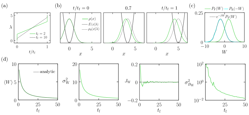
Figure 1: Model of an overdamped colloidal particle in an optical trap, at constant temperature $\beta^{-1}=1$, translated according to the work-minimizing protocol of Ref. Schmiedl and Seifert (2007). (a) Protocol $\lambda^{\star}(t)$ for two values of trajectory length $t_{\rm f}$. (b) Particle-position distribution, potential, and associated Boltzmann distribution, at three times $t$, for trajectories of length $t_{\rm f}=10$. (c) Work statistics for this protocol and its time reverse satisfy the fluctuation relation (4). (d) Mean work $\left\langle W\right\rangle$ (compared with the exact result $W^{\star}$ Schmiedl and Seifert (2007), shown as a dashed line); work variance $\sigma^{2}_{W}$; Jarzynski free-energy estimator $J_{W}$; and variance $\sigma^{2}_{{\rm B}_{W}}$ of the block average of the exponential of $J_{W}$ (note the vertical log scale). Averages and distributions are calculated over $10^{6}$ trajectories.

This problem motivates the search for nonequilibrium protocols that perform desired transformations while minimizing work or other path-extensive quantities Schmiedl and Seifert (2007); Vaikuntanathan and Jarzynski (2008); Davie et al. (2014); Blaber et al. (2021); Engel et al. (2022) . However, while protocols of this nature can involve varying temperature – such as the protocol that reverses the magnetization of the Ising model with least dissipation Rotskoff and Crooks (2015); Gingrich et al. (2016) – Eq. (1) applies only at fixed temperature.

In this paper we consider a variant of (1) that applies to protocols whose temperature can vary with time. Such variants have been derived within the framework of Hamiltonian dynamics Williams et al. (2008); Chelli (2009) or Markovian dynamics specific to the Ising model Chatelain (2007). We follow Ref. Crooks (1998) and consider a general Markovian dynamics satisfying detailed balance. If we consider the protocol to involve a set of time-varying control parameters and a time-varying reciprocal temperature $\beta(t)$, with the latter starting and ending at a value $\beta$ , then (1) is replaced by

$$\left\langle{\rm e}^{-\Omega}\right\rangle={\rm e}^{-\beta\Delta F}.$$ (2)

Here $\Omega\equiv\beta W+\beta Q-\Sigma$, where $Q$ is the heat exchanged with the bath and $-\Sigma$ is the path entropy produced by the trajectory (the instantaneous change of heat divided by the instantaneous temperature, summed over the trajectory). The quantity $\Omega-\beta\Delta F$ is the total entropy production . The angle brackets in (2) denote an average over nonequilibrium trajectories that start in equilibrium at temperature $\beta^{-1}$, that finish at the same temperature (not necessarily in equilibrium), and that otherwise involve an arbitrary change of temperature and other control parameters.

Under the same conditions, the fluctuation relation

$$P_{\rm F}(\Omega)\hskip 0.3pt{\rm e}^{-\Omega}={\rm e}^{-\beta\Delta F}P_{\rm R}(-\Omega)$$ (3)

holds. Here $P_{\rm F}(\Omega)$ denotes the probability distribution of $\Omega$ under the protocol, and $P_{\rm R}(-\Omega)$ the distribution of $-\Omega$ under the time-reversed protocol. For a fixed-temperature trajectory we have $\beta Q=\Sigma$ and so $\Omega=\beta W$, and (2) and (3) reduce to the Jarzynski equality (1) and the Crooks fluctuation relation Crooks (1999a)

$$P_{\rm F}(W)\hskip 0.3pt{\rm e}^{-\beta W}={\rm e}^{-\beta\Delta F}P_{\rm R}(-W),$$ (4)

respectively.

In what follows we sketch the derivation of (2) and (3). Details of the derivation are given in Sections S2–S4, which follow Ref. Crooks (1998) with minor notational changes . We use simulation models of a colloidal particle in an optical trap and a ferromagnet undergoing magnetization reversal to illustrate that the fluctuation relation (3) holds for varying-temperature protocols. Moreover, such protocols can give rise to smaller fluctuations of $\Omega$ and better convergence properties of (2) than do fixed-temperature protocols for $W$ and (1), allowing more accurate extraction of free-energy differences.

Sketch of derivation.— Consider a system at instantaneous temperature $\beta^{-1}(t)$. The system’s microscopic coordinates are given by a vector ${\bm{x}}$ and its energy function is $E({\bm{x}}|{\bm{\lambda}})$, where ${\bm{\lambda}}$ is a vector of control parameters. We define the protocol as the deterministic time evolution of ${\bm{\lambda}}(t)$ and $\beta(t)$. Starting in microstate ${\bm{x}}(0)={\bm{x}}_{0}$ with the parameter values ${\bm{\lambda}}(0)={\bm{\lambda}}_{0}$ and $\beta(0)=\beta_{0}$, a dynamical trajectory $\omega$ of the system consists of a series of alternating changes of the protocol, $\beta_{0},{\bm{\lambda}}_{0}\to\beta_{1},{\bm{\lambda}}_{1}\to\cdots\to\beta_{N},{\bm{\lambda}}_{N}$, and coordinates, ${\bm{x}}_{0}\to{\bm{x}}_{1}\to\cdots\to{\bm{x}}_{N}$. If $P[0\to N]$ is the probability of generating the trajectory $\omega$, and $P[0\leftarrow N]$ the probability of generating its reverse under the time-reversed protocol, then, for Markovian stochastic dynamics satisfying detailed balance, we have $P[0\to N]/P[0\leftarrow N]={\rm e}^{-\Sigma_{\omega}}$, where

$$\Sigma_{\omega}\equiv\sum_{i=0}^{N-1}\beta_{i+1}\left[E({\bm{x}}_{i+1}|{\bm{\lambda}}_{i+1})-E({\bm{x}}_{i}|{\bm{\lambda}}_{i+1})\right]$$ (5)

is (minus) the path entropy produced by $\omega$. If we assume that $\omega$ and its reverse start in thermal equilibrium with respective control-parameter values $\beta_{0},{\bm{\lambda}}_{0}$ and $\beta_{N},{\bm{\lambda}}_{N}$, where $\beta_{0}=\beta_{N}\equiv\beta$, then the path-probability ratio can be written

$$P_{0}[0\to N]{\rm e}^{-\beta W_{\omega}-\beta Q_{\omega}+\Sigma_{\omega}}={\rm e}^{-\beta\Delta F}P_{0}[0\leftarrow N].$$ (6)

Here $\Delta F$ is the Helmholtz free energy difference at temperature $\beta^{-1}$ corresponding to the change ${\bm{\lambda}}_{0}\to{\bm{\lambda}}_{N}$, and

$$W_{\omega}=\sum_{i=0}^{N-1}[E({\bm{x}}_{i}|{\bm{\lambda}}_{i+1})-E({\bm{x}}_{i}|{\bm{\lambda}}_{i})]$$ (7)

and

$$Q_{\omega}=\sum_{i=0}^{N-1}\left[E({\bm{x}}_{i+1}|{\bm{\lambda}}_{i+1})-E({\bm{x}}_{i}|{\bm{\lambda}}_{i+1})\right]$$ (8)

are the work done and heat exchanged with the bath within $\omega$.

Summing (6) over all trajectories $\omega$ gives Eq. (2) (there we have dropped the path label subscript $\omega$ on $\Omega$). Multiplying both sizes of (6) by $\delta{\left(\Omega_{\omega}-\Omega\right)}$ and summing over trajectories $\omega$ gives Eq. (3).

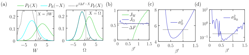
Figure 2: Trap-translation protocols run at varying temperature, with $\beta(t)=\beta^{\prime}$ for $0<t<t_{\rm f}=10$. (a) Probability distributions of $W$ and $\Omega$ for the protocol with $\beta^{\prime}=0.64$. The varying-temperature fluctuation relation (3) holds (right panel), while the work fluctuation relation (4) does not (left panel). (b) The logarithm of the estimator of (2), $J_{\Omega}$, approximates $\Delta F$, while the logarithm of the estimator of (1), $J_{W}$, does not. Fluctuations of (c) $\Omega$ and of (d) the block average of the estimator can be smaller for varying-temperature protocols ($\beta^{\prime}\neq 1$) than for constant-temperature protocols ($\beta^{\prime}=1$).

Constant-temperature protocols.— Consider a model of an overdamped colloidal particle in an optical trap Schmiedl and Seifert (2007). The particle has position $x$ and the system has energy function $E(x|\lambda)=k(t)\left(x-\lambda(t)\right)^{2}/2$, where $\lambda$ specifies the trap center. The particle undergoes the Langevin dynamics

$$\dot{x}=-\partial_{x}E(x|\lambda)+\xi(t),$$ (9)

which satisfies detailed balance with respect to the system’s energy function Crooks (1999b); Dellago et al. (1998). The noise $\xi$ satisfies $\left\langle\xi(t)\right\rangle=0$ and $\left\langle\xi(t)\xi(t^{\prime})\right\rangle=2\beta(t)^{-1}\delta(t-t^{\prime})$. Initially we set $k(t)=1$ for all $t$.

We simulate (9) using the forward Euler discretization with timestep $\Delta t=10^{-3}$. Starting in equilibrium at temperature $\beta^{-1}=1$, with the trap center at $\lambda(0)=\lambda_{0}=0$, we consider the fixed-temperature protocol that moves the trap center to a final position $\lambda(t_{\rm f})=\lambda_{\rm f}=5$, in finite time $t_{\rm f}$, and that minimizes the work averaged over many realizations of the process. This protocol has the form $\lambda^{\star}(t)=\lambda_{\rm f}(t+1)/(t_{\rm f}+2)$, for $0<t<t_{\rm f}$, with jump discontinuities at the start $(t=0)$ and end $(t=t_{\rm f})$, and produces mean work $W^{\star}=\lambda_{\rm f}^{2}/(t_{\rm f}+2)$ Schmiedl and Seifert (2007). Note that $\Delta F=0$ for this protocol, because the energy function is translated but otherwise unchanged.

In Fig. 1 we verify that work distributions produced by the protocol $\lambda^{\star}$ obey the standard relations (1) and (4). In panel (a) we show the protocol $\lambda^{\star}$ for two trajectory lengths $t_{\rm f}$. In panel (b) we show for $t_{\rm f}=10$ the time-resolved distribution of particle positions $\rho(x)$ under this protocol, together with the energy function $E(x|\lambda)$ and the associated Boltzmann distribution $\rho_{0}(x|\lambda)$. Here and subsequently we calculate distributions and averages over $10^{6}$ independent trajectories. In panel (c) we verify that the work distribution produced by this protocol and its time reverse satisfy the work-fluctuation relation (4).

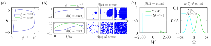
Figure 3: Ising model magnetization reversal using dissipation-minimizing fixed- and varying-temperature protocols. Protocols were determined by genetic algorithm applied to a neural network. (a) Learned protocols in parameteric form. The dotted line is the first-order phase transition line. (b) Protocols as functions of time, together with typical time-ordered snapshots. (c) Fixed-temperature protocols (for which $\Omega=\beta W$) generate large amounts of dissipation, preventing application of the standard relations (1) and (4) (left panel). Varying-temperature protocols produce much less dissipation, allowing application of (2) and (3) (right panel).

In panel (d) we compare protocols $\lambda^{\star}$ carried out for a range of trajectory lengths $t_{\rm f}$. Shown are the mean work $\left\langle W\right\rangle$; the variance $\sigma^{2}_{W}$ of the work distribution; the Jarzynski free-energy estimator $J_{W}=-\beta^{-1}\ln(N_{\rm traj}^{-1}\sum_{i=1}^{N_{\rm traj}}{\rm e}^{-\beta W_{i}})$, where $i$ labels trajectories and $N_{\rm traj}=10^{6}$; and the variance $\sigma^{2}_{{\rm B}_{W}}$ of the block average ${\rm B}_{W}=N_{\rm block}^{-1}\sum_{i=1}^{N_{\rm block}}{\rm e}^{-\beta W_{i}}$, where $N_{\rm block}=100$. The mean work satisfies $\left\langle W\right\rangle=W^{\star}$, as expected. The estimator $J_{W}$ returns $\Delta F=0$ for large values of $t_{\rm f}$, but for small values of $t_{\rm f}$ is imprecise; the fluctuation $\sigma^{2}_{W}$ is the source of this imprecision, and $\sigma^{2}_{{\rm B}_{W}}$ is one measure of its size.

Simple varying-temperature protocols.— In Fig. 2 we again consider the protocol $\lambda=\lambda^{\star}(t)$, for $t_{\rm f}=10$, but now set $\beta(t)=\beta^{\prime}$ for $0<t<t_{\rm f}$ (with $\beta(0)=\beta(t_{\rm f})=1$) and $k(t)=(1-t/t_{\rm f})k+(t/t_{\rm f})k^{\prime}$. The change of spring constant imposes a free-energy difference $\Delta F=\frac{1}{2}\ln(k^{\prime}/k)$: we choose $k^{\prime}=3k=3$, giving $\Delta F\approx 0.55$. We consider a range of $\beta^{\prime}$ either side of 1. In panel (a) we show that, as expected, the work fluctuation relation (4) is not obeyed for a varying-temperature protocol (here $\beta^{\prime}=0.64$), but the varying-temperature fluctuation relation (3) is. In panel (b) we we show that, as expected, the standard Jarzynski equality no longer applies: the green line is the free-energy estimator $J_{W}$, which for $\beta^{\prime}\neq 1$ does not equal $\Delta F$. By contrast, the estimator $J_{\Omega}=-\beta^{-1}\ln(N_{\rm traj}^{-1}\sum_{i=1}^{N_{\rm traj}}{\rm e}^{-\beta\Omega_{i}})$ provides a noisy estimate of $\Delta F$, indicating that (2) is obeyed.

In panels (c) and (d) we show, as a function of $\beta^{\prime}$, the variance $\sigma^{2}_{W}$ of $\Omega$ and the variance $\sigma^{2}_{{\rm B}_{\Omega}}$ of the block average ${\rm B}_{\Omega}=N_{\rm block}^{-1}\sum_{i=1}^{N_{\rm block}}{\rm e}^{-\beta\Omega_{i}}$, with $N_{\rm block}=100$. The minimum of the latter occurs around $\beta^{\prime}=0.65$, and is about a third of that at $\beta^{\prime}=1$ (where $\Omega=\beta W$ and the relations (2) and (3) reduce to (1) and (4)). While fluctuations tend to increase with temperature, the combination $\Omega\equiv\beta W+\beta Q-\Sigma$ and its fluctuations can be smaller than $W$ and its fluctuations. These effects compete, and for some range of $\beta^{\prime}\neq 1$ the fluctuations of $\Omega$ are smaller than those of $W$ at $\beta^{\prime}=1$, leading to better convergence of (2) than (1).

Varying-temperature protocols in the presence of a phase transition.— This difference in convergence properties is small, because the physics of the trap model does not change substantially with temperature. But when a system’s physics does change with temperature, the difference between the convergence properties of the fixed- and varying-temperature relations can be significant.

In Fig. 3 we consider the 2D ferromagnetic Ising model with fixed coupling $J=1$, on a $32\times 32$ lattice, simulated using Glauber dynamics for $t_{\rm f}=10^{3}$ Monte Carlo sweeps. Protocols start and end at parameter values $\beta(0)=\beta(t_{\rm f})=1$ and $h(0)=-h(t_{\rm f})=-1$, giving $\Delta F=0$, in which case $\Omega$ is equal to the total entropy production. We determine time-dependent protocols $\beta(t)$ and $h(t)$ for $0<t<t_{\rm f}$ by expressing these quantities using a deep neural network and training that network by genetic algorithm to minimize $\left\langle\Omega\right\rangle$ measured over $10^{4}$ independent trajectories Whitelam (2023). Protocols learned in this way effect magnetization reversal. We consider one set of learning simulations with the constraint that $\beta(t)$ remain constant, and another in which $\beta(t)$ is allowed to vary.

In panel (a) we show in parametric form the protocols learned in this way. The varying-temperature protocol avoids the critical point and the first-order phase transition line Rotskoff and Crooks (2015); Gingrich et al. (2016), while the fixed-temperature protocol is constrained to cross it. In panel (b) we show protocols as functions of time, together with time-ordered snapshots taken from typical trajectories. The fixed-temperature protocol effects nucleation and growth, accompanied by large values of dissipation: $\left\langle\Omega\right\rangle=\left\langle\beta W\right\rangle\approx 1550$. By contrast, the varying-temperature protocol is accompanied by much smaller dissipation, with $\left\langle\Omega\right\rangle\approx 11$.

As a result, distributions of work for the fixed-temperature protocol and its time-reverse are well-separated, while distributions of $\Omega$ for the varying-temperature protocol and its time reverse cross at a value that approximates $\Delta F=0$; see panel (c). Using $10^{5}$ trajectories, the free-energy estimator $J_{\Omega}$ yields a value 0.46, with block-average variance $\sigma^{2}_{{\rm B}_{\Omega}}\approx 13,700$. Thus (3) and (2) provide an accurate if imprecise measure of $\Delta F$. By contrast, if we are constrained to fixed temperature in order to apply the standard relations (1) and (4), measuring $\Delta F$ is not a realistic proposition. Fixed-temperature trajectories hundreds of times longer would be required to achieve convergence properties comparable to (2) and (3) using varying-temperature trajectories .

Conclusions.— We have shown, within the framework of Markovian stochastic dynamics satisfying detailed balance, that the relations (2) and (3) replace the Jarzynski equality (1) and Crooks work fluctuation relation (4), for trajectories influenced by a time-varying temperature that starts and ends at a value $\beta^{-1}$. We have used simulation models to show that free-energy differences can be calculated more accurately using the varying-temperature relations than the fixed-temperature ones, particularly when varying temperature gives us the freedom to avoid the large dissipation associated with a first-order phase transition. To measure the quantity $\Omega=\beta W+\beta Q-\Sigma$ that appears in (2) and (3) we must be able to measure the time-resolved heat flow, as well as total heat and work. For many experiments this will be technically demanding, but it is possible in principle.

Acknowledgments.— I thank Corneel Casert for comments on the paper. Code for the trap model can be found here tra . Code for doing neuroevolutionary learning of Ising model protocols can be found here dem , which accompanies Ref. Whitelam (2023) (for this paper we neglect the shear term, Eq. (7), used in that work). This work was performed at the Molecular Foundry at Lawrence Berkeley National Laboratory, supported by the Office of Basic Energy Sciences of the U.S. Department of Energy under Contract No. DE-AC02–05CH11231.

S1 Work fluctuations and the Jarzynski equality

To illustrate in a simple way the convergence problems of an exponential average, assume that the distribution $P(W)$ of nonequilibrium work values is Gaussian with mean $\bar{W}$ and variance $\sigma^{2}$, $P(W)\propto{\rm e}^{-(W-\bar{W})^{2}/(2\sigma^{2})}$. The average on the left-hand size of (1) can then be written

$$\left\langle{\rm e}^{-\beta W}\right\rangle\sim\int{\rm d}W{\rm e}^{-(W-W_{\rm a})^{2}/(2\sigma^{2})},$$ (S1)

which is dominated by contributions from the atypical work value $W=W_{\rm a}\equiv\bar{W}-\beta\sigma^{2}$. The probability of realizing this work value is $P(W_{\rm a})\propto{\rm e}^{-\beta^{2}\sigma^{2}/2}$, which requires a characteristic number of trajectories $\sim 1/P(W_{\rm a})\propto{\rm e}^{\beta^{2}\sigma^{2}/2}$. This quantity grows exponentially with the variance $\sigma^{2}$ of work fluctuations.

Work distributions are in general not Gaussian, but it is usually the case that the larger the fluctuations of $W$, the more trajectories are required to calculate (1).

S2 Constant-temperature protocols

S2.1 Markovian stochastic dynamics satisfying detailed balance

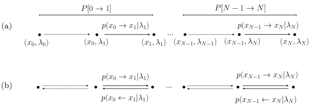
Figure S1: (a) Forward trajectory, and (b) forward-reverse trajectory pair.

In this supplement we derive the expressions (2) and (3) used in the main text, following Ref. Crooks (1998) with minor notational changes. We consider a stochastic, Markovian dynamics that satisfies detailed balance at temperature $\beta^{-1}$ with respect to the energy function $E({\bm{x}}|{\bm{\lambda}})$. Here ${\bm{x}}$ is the vector of microscopic coordinates of the system, and ${\bm{\lambda}}$ is a vector of control parameters. As shown in Fig. S1(a), a dynamical trajectory of the system involves $N$ deterministic changes of the control-parameter vector ${\bm{\lambda}}$, according to ${\bm{\lambda}}_{0}\to{\bm{\lambda}}_{1}\to\cdots\to{\bm{\lambda}}_{N}$. The system coordinates ${\bm{x}}$ evolve stochastically as ${\bm{x}}_{0}\to{\bm{x}}_{1}\to\cdots\to{\bm{x}}_{N}$. We consider these changes to occur in an alternating fashion: ${\bm{\lambda}}$ changes along dotted arrows, with work done or expended, and ${\bm{x}}$ changes along solid arrows, with heat exchanged with the thermal bath.

The probability with which the trajectory of Fig. S1(a) occurs is $P[0\to N]$, where

$$P[a\to b] = \prod_{i=a}^{b-1}P[i\to i+1]$$ (S2)

$$= \prod_{i=a}^{b-1}p({\bm{x}}_{i}\to{\bm{x}}_{i+1}|{\bm{\lambda}}_{i+1}).$$

Here $p({\bm{x}}_{i}\to{\bm{x}}_{i+1}|{\bm{\lambda}}_{i+1})$ is the probability of moving from microstate ${\bm{x}}_{i}$ to microstate ${\bm{x}}_{i+1}$, given that the control-parameter vector is ${\bm{\lambda}}_{i+1}$. The product structure of (S2) follows from the Markovian property of the dynamics.

As a convenient device, Ref. Crooks (1998) introduces the notion of a reverse trajectory, shown as the lower set of arrows in Fig. S1(b), in which ${\bm{\lambda}}$ and ${\bm{x}}$ evolve in the reverse order to the forward trajectory. The ratio of path probabilities of forward and reverse trajectories is

$$\frac{P[0\to N]}{P[0\leftarrow N]} = \prod_{i=0}^{N-1}\frac{p({\bm{x}}_{i}\to{\bm{x}}_{i+1}|{\bm{\lambda}}_{i+1})}{p({\bm{x}}_{i}\leftarrow{\bm{x}}_{i+1}|{\bm{\lambda}}_{i+1})}$$ (S3)

$$= \prod_{i=0}^{N-1}{\rm e}^{-\beta(E({\bm{x}}_{i+1}|{\bm{\lambda}}_{i+1})-E({\bm{x}}_{i}|{\bm{\lambda}}_{i+1}))}$$ (S4)

$$= {\rm e}^{-\beta Q_{0\to N}}.$$ (S5)

Here $p({\bm{x}}_{i}\leftarrow{\bm{x}}_{i+1}|{\bm{\lambda}}_{i+1})$ is the probability of moving from microstate ${\bm{x}}_{i+1}$ to microstate ${\bm{x}}_{i}$, given that the control-parameter vector is ${\bm{\lambda}}_{i+1}$, and

$$Q_{0\to N}=\sum_{i=0}^{N-1}\left[E({\bm{x}}_{i+1}|{\bm{\lambda}}_{i+1})-E({\bm{x}}_{i}|{\bm{\lambda}}_{i+1})\right]$$ (S6)

is the heat exchanged with the bath along the forward trajectory. In the main text we use the subscript $\omega$ to indicate a trajectory-dependent quantity. Here we use the more detailed notation $0\to N$, so that we can in describe portions of the trajectory using the notation $i\to j$. The passage from (S3) to (S4) follows from the fact that the dynamics satisfies detailed balance. Eq. (S5) is a statement of microscopic reversibility: it is guaranteed if the dynamics satisfies detailed balance, but also holds if the dynamics satisfied global balance and not detailed balance.

Given a control-parameter vector ${\bm{\lambda}}_{i}$, the likelihood of observing microstate ${\bm{x}}_{j}$ in thermal equilibrium is

$$\rho({\bm{x}}_{j}|{\bm{\lambda}}_{i})={\rm e}^{\beta(F_{\beta}({\bm{\lambda}}_{i})-E({\bm{x}}_{j}|{\bm{\lambda}}_{i}))},$$ (S7)

where

$$F_{\beta}({\bm{\lambda}}_{i})=-\beta^{-1}\ln\sum_{\bm{x}}{\rm e}^{-\beta E({\bm{x}}|{\bm{\lambda}}_{i})}$$ (S8)

is the Helmholtz free energy of the system under control-parameter vector ${\bm{\lambda}}_{i}$ (we shall drop subscript labels $\beta$ on $F$ unless considering free energies calculated at different temperatures). If we assume that forward and reverse trajectories each start in thermal equilibrium under respective control-parameter values ${\bm{\lambda}}_{0}$ and ${\bm{\lambda}}_{N}$, then the path-probability ratio (S3) becomes

$$\frac{\rho({\bm{x}}_{0}|{\bm{\lambda}}_{0})P[0\to N]}{P[0\leftarrow N]\rho({\bm{x}}_{N}|{\bm{\lambda}}_{N})}={\rm e}^{-\beta(\Delta F_{0\to N}-\Delta E_{0\to N}+Q_{0\to N})},$$ (S9)

where $\Delta F_{0\to N}\equiv F({\bm{\lambda}}_{N})-F({\bm{\lambda}}_{0})$ and $\Delta E_{0\to N}\equiv E({\bm{x}}_{N}|{\bm{\lambda}}_{N})-E({\bm{x}}_{0}|{\bm{\lambda}}_{0})$. Using the first law of thermodynamics,

$$Q_{0\to N}+W_{0\to N}=\Delta E_{0\to N},$$ (S10)

where

$$W_{0\to N}=\sum_{i=0}^{N-1}[E({\bm{x}}_{i}|{\bm{\lambda}}_{i+1})-E({\bm{x}}_{i}|{\bm{\lambda}}_{i})]$$ (S11)

is the work done along the forward trajectory, (S9) can be written

$$\frac{\rho({\bm{x}}_{0}|{\bm{\lambda}}_{0})P[0\to N]}{P[0\leftarrow N]\rho({\bm{x}}_{N}|{\bm{\lambda}}_{N})}={\rm e}^{-\beta(\Delta F_{0\to N}-W_{0\to N})}.$$ (S12)

It will be convenient to write (S12) as

$$\rho({\bm{x}}_{0}|{\bm{\lambda}}_{0}) P [0\to N]{\rm e}^{-\beta W_{0\to N}}$$ (S13)

$$= {\rm e}^{-\beta\Delta F_{0\to N}}P[0\leftarrow N]\rho({\bm{x}}_{N}|{\bm{\lambda}}_{N}).$$

S2.2 Jarzynski equality

Summing (S13) over all possible trajectories $\{{\bm{x}}\}$ gives

$$\sum_{\{{\bm{x}}\}}\rho({\bm{x}}_{0}|{\bm{\lambda}}_{0})P[0\to N]{\rm e}^{-\beta W_{0\to N}}$$ (S14)

$$= {\rm e}^{-\beta\Delta F_{0\to N}}\sum_{\{{\bm{x}}\}}P[0\leftarrow N]\rho({\bm{x}}_{N}|{\bm{\lambda}}_{N}).$$

The sum on the right-hand side of (S14) is unity, by normalization of probabilities, and we can write what remains as

$$\left\langle{\rm e}^{-\beta W_{0\to N}}\right\rangle_{{\bm{\lambda}}_{0}\to{\bm{\lambda}}_{N}}={\rm e}^{-\beta\Delta F_{0\to N}}.$$ (S15)

The angle brackets in (S15) denotes an average over all forward trajectories, starting from thermal equilibrium under the control-parameter vector ${\bm{\lambda}}_{0}$. This completes the proof of the Jarzynski equality given in Ref. Crooks (1998), for a Markovian, stochastic dynamics satisfying detailed balance. Only the starting point of the forward trajectory is in thermal equilibrium; no subsequent points on the trajectory, including the final one, need be in equilibrium. The reverse trajectory is introduced as a device to ensure a convenient cancellation of terms in the derivation of (S15), but no reverse trajectories need be considered for its calculation.

In the remainder of Section S2 we consider some special cases and limits of the Jarzynski equality.

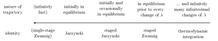
Figure S2: Summary of the results of Section S2, relating the nature of the forward trajectory of Fig. S1(a) to the identity that applies to it. The line points in the direction of increasing rate of transformation.

S2.3 Staged Jarzynski equality

Assume now that forward and reverse trajectories attain equilibrium when the control-parameter vector is ${\bm{\lambda}}_{i}$, where $0<i<N$. To enforce this assumption we insert the factor $\rho({\bm{x}}_{i}|{\bm{\lambda}}_{i})$ in the numerator and denominator of (S12), giving

$$\frac{\rho({\bm{x}}_{0}|{\bm{\lambda}}_{0})P[0\to i]\rho({\bm{x}}_{i}|{\bm{\lambda}}_{i})P[i\to N]}{P[0\leftarrow i]\rho({\bm{x}}_{i}|{\bm{\lambda}}_{i})P[i\leftarrow N]\rho({\bm{x}}_{N}|{\bm{\lambda}}_{N})}.$$ (S16)

The value of (S16) is again equal to ${\rm e}^{-\beta(\Delta F_{0\to N}-W_{0\to N})}$, but forward and reverse trajectories now possess a constraint not present in the previous case. This constraint could be enforced by having a time-varying protocol that pauses at the value ${\bm{\lambda}}_{i}$ for as long as required to achieve equilibrium. However, we could also consider the expression (S16) to refer to two sets of trajectory pairs that involve the portions $0\to i$ and $i\to N$ of the original trajectory, respectively. These trajectory pairs start in equilibrium and possess no additional constraints. The form of (S16) consistent with this assumption is

$$\frac{\rho({\bm{x}}_{0}|{\bm{\lambda}}_{0})P[0\to i]}{P[0\leftarrow i]\rho({\bm{x}}_{i}|{\bm{\lambda}}_{i})}\cdot\frac{\rho({\bm{x}}_{i}|{\bm{\lambda}}_{i})P[i\to N]}{P[i\leftarrow N]\rho({\bm{x}}_{N}|{\bm{\lambda}}_{N})},$$ (S17)

the two factors in (S17) corresponding to the two trajectory pairs. The arguments leading to (S15) can be applied separately to these two factors, yielding

$$\left\langle{\rm e}^{-\beta W_{0\to i}}\right\rangle_{{\bm{\lambda}}_{0}\to{\bm{\lambda}}_{i}}\left\langle{\rm e}^{-\beta W_{i\to N}}\right\rangle_{{\bm{\lambda}}_{i}\to{\bm{\lambda}}_{N}} = {\rm e}^{-\beta\Delta F_{0\to i}}{\rm e}^{-\beta\Delta F_{i\to N}}$$ (S18)

$$= {\rm e}^{-\beta\Delta F_{0\to N}},$$

where the two angle brackets denote averages over all trajectories, starting in equilibrium under control-parameter values ${\bm{\lambda}}_{0}$ and ${\bm{\lambda}}_{i}$, respectively.

Eq. (S18) is the statement that the Jarzynski equality (S15) can be evaluated by staging Pohorille et al. (2010), dividing a single trajectory (which starts in equilibrium but need not be in equilibrium subsequently) into shorter trajectories (each of which starts in equilibrium but need not be in equilibrium subsequently). This is obvious on physical grounds, given that the Jarzynski equality is a method for evaluating free-energy differences, and it applies to trajectories of arbitrary length.

S2.4 Staged Zwanzig formula for free-energy perturbation

A special case arises when we insert, in the numerator and denominator of (S12), factors of $\rho({\bm{x}}_{i}|{\bm{\lambda}}_{i})$ for all values of $i$, so assuming that both trajectories attain equilibrium between each variation of the control-parameter vector ${\bm{\lambda}}$ and the next. In this case (S12) becomes

$$\prod_{i=0}^{N-1}\frac{\rho({\bm{x}}_{i}|{\bm{\lambda}}_{i})P[i\to i+1]}{P[i\leftarrow i+1]\rho({\bm{x}}_{i+1}|{\bm{\lambda}}_{i+1})}={\rm e}^{-\beta\Delta F_{0\to N}}.$$ (S19)

Each factor on the left-hand side of (S19) is

$$\frac{\rho({\bm{x}}_{i}|{\bm{\lambda}}_{i})P[i\to i+1]}{P[i\leftarrow i+1]\rho({\bm{x}}_{i+1}|{\bm{\lambda}}_{i+1})} = {\rm e}^{-\beta(E({\bm{x}}_{i}|{\bm{\lambda}}_{i})-E({\bm{x}}_{i}|{\bm{\lambda}}_{i+1}))}$$ (S20)

$$\times {\rm e}^{-\beta(F({\bm{\lambda}}_{i+1})-F({\bm{\lambda}}_{i}))}.$$

The right-hand side of (S20) depends on the energy at a single coordinate ${\bm{x}}_{i}$ only, and so the notion of an explicit dynamics is absent. Rearranging (S20) and summing over trajectories $\{{\bm{x}}\}$ gives

$$\sum_{{\bm{x}}_{i}}\rho({\bm{x}}_{i}|{\bm{\lambda}}_{i}){\rm e}^{-\beta(E({\bm{x}}_{i}|{\bm{\lambda}}_{i+1})-E({\bm{x}}_{i}|{\bm{\lambda}}_{i}))}\sum_{{\bm{x}}_{i+1}}P[i\to i+1]$$

$$= {\rm e}^{-\beta(F({\bm{\lambda}}_{i+1})-F({\bm{\lambda}}_{i}))}\sum_{{\bm{x}}_{i},{\bm{x}}_{i+1}}P[i\leftarrow i+1]\rho({\bm{x}}_{i+1}|{\bm{\lambda}}_{i+1}),$$

which can be written

$$\left\langle{\rm e}^{-\beta(E({\bm{x}}|{\bm{\lambda}}_{i+1})-E({\bm{x}}|{\bm{\lambda}}_{i}))}\right\rangle_{{\bm{\lambda}}_{i}}={\rm e}^{-\beta\Delta F_{i\to i+1}}.$$ (S21)

Here the angle brackets $\left\langle(\cdot)\right\rangle_{{\bm{\lambda}}_{i}}$ denote an equilibrium average $\sum_{\bm{x}}\rho({\bm{x}}|{\bm{\lambda}}_{i})(\cdot)$ under the control-parameter vector ${\bm{\lambda}}_{i}$. Eq. (S21) is the exponential of the Zwanzig formula for free-energy perturbation Zwanzig (1954). Using (S21), (S19) can be written

$$\Delta F_{0\to N}=-\beta^{-1}\sum_{i=0}^{N-1}\ln\left\langle{\rm e}^{-\beta(E({\bm{x}}|{\bm{\lambda}}_{i+1})-E({\bm{x}}|{\bm{\lambda}}_{i}))}\right\rangle_{{\bm{\lambda}}_{i}},$$ (S22)

which is a staged version of Zwanzig formula for $N$ changes of the control-parameter vector ${\bm{\lambda}}$. To calculate (S22), it is natural to consider $N$ independent trajectories that all begin in equilibrium and consist of a single change of the control-parameter vector.

It was shown in Ref. Jarzynski (1997) that the Jarzynski equality reduces to the Zwanzig formula

$$\Delta F_{0\to N}=-\beta^{-1}\ln\left\langle{\rm e}^{-\beta(E({\bm{x}}|{\bm{\lambda}}_{0})-E({\bm{x}}|{\bm{\lambda}}_{N}))}\right\rangle_{{\bm{\lambda}}_{0}}$$ (S23)

for a single, instantaneous change of the control-parameter vector from ${\bm{\lambda}}_{0}\to{\bm{\lambda}}_{N}$. Eq. (S22) is the staged variant of this expression: (S22) applies if the transformation is done in well-separated stages, with the system coming to equilibrium after each control-parameter change.

S2.5 Thermodynamic integration

If we further assume that the trajectory involves only small changes of the control-parameter vector, ${\bm{\lambda}}_{i+1}={\bm{\lambda}}_{i}+\delta{\bm{\lambda}}$, such that

$$E({\bm{x}}|{\bm{\lambda}}_{i+1})\approx E({\bm{x}}|{\bm{\lambda}}_{i})+\delta{\bm{\lambda}}\cdot\frac{\partial E({\bm{x}}|{\bm{\lambda}})}{\partial{\bm{\lambda}}}|_{{\bm{\lambda}}={\bm{\lambda}}_{i}},$$ (S24)

then (S22) becomes

$$\Delta F_{0\to N} \approx -\beta^{-1}\sum_{i=0}^{N-1}\ln\left(1-\beta\delta{\bm{\lambda}}\cdot\left\langle\frac{\partial E({\bm{x}}|{\bm{\lambda}})}{\partial{\bm{\lambda}}}\right\rangle_{{\bm{\lambda}}_{i}}\right)$$ (S25)

$$\approx \sum_{i=0}^{N-1}\delta{\bm{\lambda}}\cdot\left\langle\frac{\partial E({\bm{x}}|{\bm{\lambda}})}{\partial{\bm{\lambda}}}\right\rangle_{{\bm{\lambda}}_{i}}.$$

In the limit of a large number $N\to\infty$ of vanishingly small changes $\delta{\bm{\lambda}}\to 0$ we can write the above as

$$\Delta F_{0\to N}=\int_{{\bm{\lambda}}_{0}}^{{\bm{\lambda}}_{N}}{\rm d}{\bm{\lambda}}\cdot\left\langle\frac{\partial E({\bm{x}}|{\bm{\lambda}})}{\partial{\bm{\lambda}}}\right\rangle_{\bm{\lambda}},$$ (S26)

which is the formula for thermodynamic integration Kirkwood (1935); Frenkel and Smit (2001). In Ref. Jarzynski (1997) it was shown, within the framework of Hamiltonian dynamics, that thermodynamic integration is recovered from the Jarzynski equality in the limit of an infinitely slow transformation.

S2.6 Summary of this section

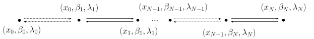
Figure S3: Modification of the protocol of Fig. S1 to permit a time-varying temperature $\beta_{i}^{-1}$.

Fig. S2 summarizes the results of Section S2. In Ref. Crooks (1998) it was shown that consideration of forward and reverse trajectory-pairs permits a simple proof of the Jarzynski equality Jarzynski (1997), Eq. (S15), for trajectories of a Markovian stochastic dynamics that satisfies detailed balance, provided that these trajectories begin in thermal equilibrium with respect to the initial value of the control-parameter vector. We have summarized this proof in Section S2.1 and Section S2.2. Using the same framework we have shown in Section S2.3 that if trajectories also attain thermal equilibrium with other values of the control-parameter vector then we recover the (physically obvious) statement that the Jarzynski equality can be evaluated in a staged way. In Section S2.4 we show that if trajectories attain thermal equilibrium after all changes of the control-parameter vector then the same considerations yield a staged version of the Zwanzig formula Zwanzig (1954) for free-energy perturbation, Eq. (S22). (The single-stage Zwanzig formula is recovered in the limit of a single, instantaneous change of ${\bm{\lambda}}$ Jarzynski (1997).) In Section S2.5 we show that if, in addition, the control-parameter vector is changed in a large number of infinitesimally small steps, we recover the formula for thermodynamic integration, Eq. (S26). (The same formula is recovered in the limit of an infinitely slow transformation with the framework of Hamiltonian dynamics Jarzynski (1997).)

S3 Varying-temperature protocols

In this section we modify the proof of Section S2 to allow for a time-varying reciprocal temperature $\beta$, such that $\beta_{0}\to\beta_{1}\to\cdots\to\beta_{N}$ along a trajectory. We change $\beta$ in step with the control-parameter vector ${\bm{\lambda}}$, as shown in Fig. S3, and so where ${\bm{\lambda}}={\bm{\lambda}}_{i}$ we have $\beta=\beta_{i}$. We note that the microscopic energies $E({\bm{x}}_{i}|{\bm{\lambda}}_{i})$ could in principle be temperature dependent.

Under this new protocol, Eq. (S5) reads

$$\frac{P[0\to N]}{P[0\leftarrow N]} = \prod_{i=0}^{N-1}\frac{p({\bm{x}}_{i}\to{\bm{x}}_{i+1}|{\bm{\lambda}}_{i+1})}{p({\bm{x}}_{i}\leftarrow{\bm{x}}_{i+1}|{\bm{\lambda}}_{i+1})}$$ (S27)

$$= \prod_{i=0}^{N-1}{\rm e}^{-\beta_{i+1}(E({\bm{x}}_{i+1}|{\bm{\lambda}}_{i+1})-E({\bm{x}}_{i}|{\bm{\lambda}}_{i+1}))}$$

$$= {\rm e}^{-\Sigma_{0\to N}},$$

where

$$\Sigma_{0\to N}\equiv\sum_{i=0}^{N-1}\beta_{i+1}\left[E({\bm{x}}_{i+1}|{\bm{\lambda}}_{i+1})-E({\bm{x}}_{i}|{\bm{\lambda}}_{i+1})\right]$$ (S28)

is (minus) the path entropy along the forward trajectory (i.e. neglecting the endpoint distributions). Eq. (S28) is an explicit realization of the path term appearing in the generic form $\Delta S_{\rm baths}$ given in Eq. (1.18) of Ref. Crooks (1999b).

For a varying-temperature protocol, Eq. (S9) becomes

$$\frac{\rho({\bm{x}}_{0}|{\bm{\lambda}}_{0})P[0\to N]}{P[0\leftarrow N]\rho({\bm{x}}_{N}|{\bm{\lambda}}_{N})} = {\rm e}^{\beta_{0}F_{\beta_{0}}({\bm{\lambda}}_{0})-\beta_{N}F_{\beta_{N}}({\bm{\lambda}}_{N})}$$

$$\times {\rm e}^{\beta_{N}E({\bm{x}}_{N}|{\bm{\lambda}}_{N})-\beta_{0}E({\bm{x}}_{0}|{\bm{\lambda}}_{0})-\Sigma_{0\to N}}.$$

Because our goal is to evaluate free-energy differences at fixed temperature $\beta^{-1}$, we now specify that the temperatures at the start and end of the trajectory are equal, $\beta_{0}=\beta_{N}\equiv\beta$ (we allow general $\beta_{i}>0$ for $0<i<N$). In this case the free-energy difference appearing in the first line of (S3) is again $-\beta\Delta F_{0\to N}$, and the difference of internal energies given on the second line of (S3) becomes $\beta\Delta E_{0\to N}$. This can be eliminated in favor of the path-dependent combination $\beta(W_{0\to N}+Q_{0\to N})$: $\beta$ times the sum of (S6) and (S11) is equal to $\beta\Delta E_{0\to N}$, whether or not the time-dependent temperature along the path is equal to the temperature at the trajectory endpoints.

Thus, for a varying-temperature trajectory that starts and ends at temperature $\beta^{-1}$, Eq. (S3) can be written

$$\frac{\rho({\bm{x}}_{0}|{\bm{\lambda}}_{0})P[0\to N]}{P[0\leftarrow N]\rho({\bm{x}}_{N}|{\bm{\lambda}}_{N})} = {\rm e}^{-\beta\Delta F_{0\to N}+\beta\Delta E_{0\to N}-\Sigma_{0\to N}}$$

$$= {\rm e}^{-\beta\Delta F_{0\to N}+\beta(W_{0\to N}+Q_{0\to N})-\Sigma_{0\to N}},$$

giving

$$\rho({\bm{x}}_{0}|{\bm{\lambda}}_{0})P[0\to N]{\rm e}^{-\beta W_{0\to N}-\beta Q_{0\to N}+\Sigma_{0\to N}}$$

$$=P[0\leftarrow N]\rho({\bm{x}}_{N}|{\bm{\lambda}}_{N}){\rm e}^{-\beta\Delta F_{0\to N}}.$$ (S31)

Summing (S3) over all trajectories $\{{\bm{x}}\}$ gives

$$\left\langle{\rm e}^{-\Omega_{0\to N}}\right\rangle_{{\bm{\lambda}}_{0}\to{\bm{\lambda}}_{N}}={\rm e}^{-\beta\Delta F_{0\to N}},$$ (S32)

where

$$\Omega_{0\to N}\equiv\beta W_{0\to N}+\beta Q_{0\to N}-\Sigma_{0\to N}.$$ (S33)

The angle brackets in (S32) denotes an average over nonequilibrium trajectories of fixed but arbitrary length that start in equilibrium with reciprocal temperature $\beta_{0}=\beta$ and control-parameter vector ${\bm{\lambda}}_{0}$, end with reciprocal temperature $\beta_{N}=\beta$ and control-parameter vector ${\bm{\lambda}}_{N}$, and otherwise involve an arbitrary time-dependent variation of $\beta_{i}$ and ${\bm{\lambda}}_{i}$.

Eq. (S32), Eq. (2) of the main text, is a variant of the Jarzynski equality (S15) that is valid for a varying-temperature protocol with equal start- and end temperatures.

The Jensen inequality applied to (S32) yields $\left\langle\Omega_{0\to N}\right\rangle\geq\beta\Delta F$, the statement that the total entropy production is nonnegative. This is an expression of the second law of thermodynamics, similar to the statement $\left\langle W\right\rangle\geq\Delta F$ that results from Jensen’s inequality applied to the Jarzynski equality.

S4 Fluctuation relations

S4.1 Fixed temperature

In this section we consider the fluctuation relations that correspond to the expressions (S15) and (S32). Thus far, reverse trajectories have been considered as a device to derive the Jarzynski equality and related identities, but evaluation of those identities requires only the generation forward trajectories. In this subsection we will consider expressions (again derived using reverse trajectories as a convenient device) that refer explicitly to the ensemble of trajectories generated using the time-reversed protocol.

Crooks’ work fluctuation relation Crooks (1999a) follows by multiplying (S13) by $\delta{\left(W_{0\to N}-W\right)}$ and summing over all possible trajectories $\{{\bm{x}}\}$. The result is

$$\sum_{\{{\bm{x}}\}}\delta{\left(W_{0\to N}-W\right)}\rho({\bm{x}}_{0}|{\bm{\lambda}}_{0})P[0\to N]{\rm e}^{-\beta W_{0\to N}}$$

$$= {\rm e}^{-\beta\Delta F_{0\to N}}\sum_{\{{\bm{x}}\}}\delta{\left(W_{0\to N}-W\right)}P[0\leftarrow N]\rho({\bm{x}}_{N}|{\bm{\lambda}}_{N}),$$

which can be written

$$P_{\rm F}(W)\,{\rm e}^{-\beta W}={\rm e}^{-\beta\Delta F_{0\to N}}P_{\rm R}(-W).$$ (S35)

Here $P_{\rm F}(W)$ is the probability of observing work value $W_{0\to N}=W$ for a forward trajectory, and $P_{\rm R}(-W)$ is the probability of observing work value $W_{N\to 0}=-W$ for a trajectory generated by the time-reversed protocol (note that $W_{0\to N}=-W_{N\to 0}$). Integrating (S35) over $W$ gives (S15).

S4.2 Varying temperature

The detailed fluctuation relation corresponding to (S32) follows by multiplying (S3) by $\delta{\left(W_{0\to N}-W\right)}\delta{\left(Q_{0\to N}-Q\right)}\delta{\left(\Sigma_{0\to N}-\Sigma\right)}$ and summing over $\{{\bm{x}}\}$, and is

$$P_{\rm F}(W, Q ,\Sigma)\,{\rm e}^{-\beta W-\beta Q+\Sigma}$$ (S36)

$$= {\rm e}^{-\beta\Delta F_{0\to N}}P_{\rm R}(-W,-Q,-\Sigma).$$

Here $P_{\rm F}(W,Q,\Sigma)$ is the joint probability of observing the values $(W_{0\to N},Q_{0\to N},\Sigma_{0\to N})=(W,Q,\Sigma)$ for a forward trajectory, and similarly for $P_{\rm R}(-W,-Q,-\Sigma)$ is is the joint probability of observing the values $(W_{0\to N},Q_{0\to N},\Sigma_{0\to N})=(-W,-Q,-\Sigma)$ for a trajectory generated by the time-reversed protocol.

The simple fluctuation relation associated with (S32) follows by multiplying both sizes of (S3) by $\delta{\left(\Omega_{0\to N}-\Omega\right)}$ and summing over $\{{\bm{x}}\}$, and is

$$P_{\rm F}(\Omega)\,{\rm e}^{-\Omega}={\rm e}^{-\beta\Delta F_{0\to N}}P_{\rm R}(-\Omega).$$ (S37)

Here $P_{\rm F}(\Omega)$ is the probability of observing the value $\Omega_{0\to N}=\Omega$ for a forward trajectory, and $P_{\rm R}(-\Omega)$ is the probability of observing the value $\Omega_{N\to 0}=-\Omega$ for a reverse trajectory (note that $\Omega_{0\to N}=-\Omega_{N\to 0}$). Eq. (S37) is Eq. (3) of the main text. Integrating (S37) over $\Omega$ gives (S32).

For a constant-temperature protocol, $\beta Q=\Sigma$ and $\Omega=\beta W$, and both (S36) and (S37) reduce to (S35).

Finally, note that $\Omega-\Delta F_{0\to N}$ is the total entropy production, and (S37) can be considered a special case (one where the temperatures at the trajectory endpoints are equal) of a varying-temperature version of the entropy-production fluctuation theorem Evans and Searles (2002).

References

- Jarzynski (1997) Christopher Jarzynski, “Nonequilibrium equality for free energy differences,” Physical Review Letters 78, 2690 (1997).
- Jarzynski (2008) C Jarzynski, “Nonequilibrium work relations: foundations and applications,” The European Physical Journal B 64, 331–340 (2008).
- Jarzynski (2006) Christopher Jarzynski, “Rare events and the convergence of exponentially averaged work values,” Physical Review E 73, 046105 (2006).
- Hummer and Szabo (2010) Gerhard Hummer and Attila Szabo, “Free energy profiles from single-molecule pulling experiments,” Proceedings of the National Academy of Sciences 107, 21441–21446 (2010).
- Rohwer et al. (2015) Christian M Rohwer, Florian Angeletti, and Hugo Touchette, “Convergence of large-deviation estimators,” Physical Review E 92, 052104 (2015).
- Schmiedl and Seifert (2007) Tim Schmiedl and Udo Seifert, “Optimal finite-time processes in stochastic thermodynamics,” Physical Review Letters 98, 108301 (2007).
- Vaikuntanathan and Jarzynski (2008) Suriyanarayanan Vaikuntanathan and Christopher Jarzynski, “Escorted free energy simulations: Improving convergence by reducing dissipation,” Physical Review Letters 100, 190601 (2008).
- Davie et al. (2014) Stuart J Davie, Owen G Jepps, Lamberto Rondoni, James C Reid, and Debra J Searles, “Applicability of optimal protocols and the Jarzynski equality,” Physica Scripta 89, 048002 (2014).
- Blaber et al. (2021) Steven Blaber, Miranda D Louwerse, and David A Sivak, “Steps minimize dissipation in rapidly driven stochastic systems,” Physical Review E 104, L022101 (2021).
- Engel et al. (2022) Megan C Engel, Jamie A Smith, and Michael P Brenner, “Optimal control of nonequilibrium systems through automatic differentiation,” arXiv preprint arXiv:2201.00098 (2022).
- Note (1) Minimizing work does not necessarily minimize the fluctuations of work, but there is usually a strong correlation between these things. See e.g. panel (d) of Fig. 1.
- Rotskoff and Crooks (2015) Grant M Rotskoff and Gavin E Crooks, “Optimal control in nonequilibrium systems: Dynamic riemannian geometry of the ising model,” Physical Review E 92, 060102 (2015).
- Gingrich et al. (2016) Todd R Gingrich, Grant M Rotskoff, Gavin E Crooks, and Phillip L Geissler, “Near-optimal protocols in complex nonequilibrium transformations,” Proceedings of the National Academy of Sciences 113, 10263–10268 (2016).
- Williams et al. (2008) Stephen R Williams, Debra J Searles, and Denis J Evans, “Nonequilibrium free-energy relations for thermal changes,” Physical review letters 100, 250601 (2008).
- Chelli (2009) Riccardo Chelli, “Nonequilibrium work relations for systems subject to mechanical and thermal changes,” The Journal of Chemical Physics 130 (2009).
- Chatelain (2007) Christophe Chatelain, “A temperature-extended Jarzynski relation: application to the numerical calculation of surface tension,” Journal of Statistical Mechanics: Theory and Experiment 2007, P04011 (2007).
- Crooks (1998) Gavin E Crooks, “Nonequilibrium measurements of free energy differences for microscopically reversible markovian systems,” Journal of Statistical Physics 90, 1481–1487 (1998).
- Note (2) with no time argument or subscript denotes the fixed reciprocal temperature at the start and end of the trajectory: we want to estimate the value appearing in (1) by allowing the system at intermediate times to have a value that may be different to the end-point value .
- Note (3) Eq. (2) can be considered a special case – one where the temperatures at the trajectory endpoints are equal – of a varying-temperature version of the entropy-production fluctuation theorem Evans and Searles (2002); Seifert (2012).
- Crooks (1999a) Gavin E Crooks, “Entropy production fluctuation theorem and the nonequilibrium work relation for free energy differences,” Physical Review E 60, 2721 (1999a).
- Note (4) We also show that the Jarzynski equality becomes the staged Zwanzig formula for free-energy perturbation if the trajectory remains in equilibrium, and becomes the formula for thermodynamic integration if, in addition, the control parameters change in infinitesimal increments; related limiting forms were derived in Ref. Jarzynski (1997) within the framework of Hamiltonian dynamics.
- Crooks (1999b) Gavin E. Crooks, Excursions in statistical dynamics (PhD Thesis, University of California, Berkeley, 1999).
- Dellago et al. (1998) Christoph Dellago, Peter G Bolhuis, and David Chandler, “Efficient transition path sampling: Application to lennard-jones cluster rearrangements,” The Journal of chemical physics 108, 9236–9245 (1998).
- Whitelam (2023) Stephen Whitelam, “Demon in the machine: learning to extract work and absorb entropy from fluctuating nanosystems,” Physical Review X 13, 021005 (2023).
- Note (5) For the Ising model we could change at fixed to mimic temperature variation. Our model study is carried out to represent an experiment in which we cannot change the microscopic parameters of a material, but we can use temperature as a control parameter to take us across a phase boundary.
- (26) https://github.com/swhitelam/trap.
- (27) https://github.com/swhitelam/demon.
- Evans and Searles (2002) Denis J Evans and Debra J Searles, “The fluctuation theorem,” Advances in Physics 51, 1529–1585 (2002).
- Seifert (2012) Udo Seifert, “Stochastic thermodynamics, fluctuation theorems and molecular machines,” Reports on progress in physics 75, 126001 (2012).
- Pohorille et al. (2010) Andrew Pohorille, Christopher Jarzynski, and Christophe Chipot, “Good practices in free-energy calculations,” The Journal of Physical Chemistry B 114, 10235–10253 (2010).
- Zwanzig (1954) Robert W Zwanzig, “High-temperature equation of state by a perturbation method. I. Nonpolar gases,” The Journal of Chemical Physics 22, 1420–1426 (1954).
- Kirkwood (1935) John G Kirkwood, “Statistical mechanics of fluid mixtures,” The Journal of Chemical Physics 3, 300–313 (1935).
- Frenkel and Smit (2001) Daan Frenkel and Berend Smit, Understanding molecular simulation: from algorithms to applications, Vol. 1 (Academic Press, 2001).