Analyzing Collections and Pipelines of Futures with Graph Types
Francis Rinaldi
frinaldi@hawk.iit.eduIllinois Institute of TechnologyUSA, june wunder
jwunder@bu.eduBoston UniversityUSA, Arthur Azevedo de Amorim
aaavcs@rit.eduRochester Institute of TechnologyUSA and Stefan K. Muller
smuller2@iit.eduIllinois Institute of TechnologyUSA
Pipelines and Beyond: Graph Types for ADTs with Futures
Francis Rinaldi
frinaldi@hawk.iit.eduIllinois Institute of TechnologyUSA, june wunder
jwunder@bu.eduBoston UniversityUSA, Arthur Azevedo de Amorim
aaavcs@rit.eduRochester Institute of TechnologyUSA and Stefan K. Muller
smuller2@iit.eduIllinois Institute of TechnologyUSA
Abstract.
Parallel programs are frequently modeled as dependency or cost graphs, which can be used to detect various bugs, or simply to visualize the parallel structure of the code. However, such graphs reflect just one particular execution and are typically constructed in a post-hoc manner. Graph types, which were introduced recently to mitigate this problem, can be assigned statically to a program by a type system and compactly represent the family of all graphs that could result from the program.
Unfortunately, prior work is restricted in its treatment of futures, an increasingly common and especially dynamic form of parallelism. In short, each instance of a future must be statically paired with a vertex name. Previously, this led to the restriction that futures could not be placed in collections or be used to construct data structures. Doing so is not a niche exercise: such structures form the basis of numerous algorithms that use forms of pipelining to achieve performance not attainable without futures. All but the most limited of these examples are out of reach of prior graph type systems.
In this paper, we propose a graph type system that allows for almost arbitrary combinations of futures and recursive data types. We do so by indexing datatypes with a type-level vertex structure, a codata structure that supplies unique vertex names to the futures in a data structure. We prove the soundness of the system in a parallel core calculus annotated with vertex structures and associated operations. Although the calculus is annotated, this is merely for convenience in defining the type system. We prove that it is possible to annotate arbitrary recursive types with vertex structures, and show using a prototype inference engine that these annotations can be inferred from OCaml-like source code for several complex parallel algorithms.
††copyright: none
1. Introduction
Decades of work on reasoning about parallel programs have focused
on computation or cost graphs, directed graphs that
represent the dependencies of threads.
Computation graphs are a convenient target for analysis because they abstract
away details of the program, language, and even the parallelism features that
were used, while still capturing enough information about the relationships
between threads to perform many useful analyses.
For example, computation graphs have been used to study
deadlock (Cogumbreiro et al., 2018),
data races (Banerjee
et al., 2006),
priority inversions (Babaoğlu et al., 1993) and
evaluation cost (Blelloch and
Greiner, 1995, 1996).
To analyze such properties, it is desirable to calculate the computation graph
of a program statically, at compile time or analysis time.
Doing so is often possible in languages and threading libraries for
coarse-grained parallelism, such as pthreads,
where thread creation and synchronization are expensive and rare.
Much recent interest in parallel programming, however, has been in the area
of fine-grained parallelism, in which threads are created cheaply and
eagerly, often based on runtime conditions.
For example, a program might fork at each level of a divide-and-conquer
algorithm, or a web server might spawn a new thread to handle every incoming
request asynchronously.
Reasoning statically about the dependency structure of fine-grained parallel
programs is difficult because of the highly dynamic nature of thread creation
and synchronization in these programs.
This difficulty is compounded when programs use futures and related
abstractions for fine-grained parallelism, which are becoming increasingly
popular and have been made available in Python, Scala, Rust, and the most recent
release of OCaml (Sivaramakrishnan
et al., 2020), among other
languages.
Essentially, a future is a first-class handle to an asynchronous computation.
The result of the computation can be demanded via a
force or touch operation, which blocks if the result
is not yet available.
Because futures run in separate threads,
we can model each future as its own vertex
in the computation graph of a program. Edges leading into track the
intermediate results used to compute the future, and when we touch the future,
we add an edge from to the thread where the touch happened.
Futures may be passed around a program arbitrarily and end up being touched in a
very different part of the program from where it was spawned, leading to great
power and flexibility but also complex computation graphs which are difficult to
reason about.
To address the difficulty of predicting parallel dependences in fine-grained
parallel programs, especially those with futures,
Muller (2022) introduced the notion of graph
types, which statically overapproximate the set of computation graphs that
might result from running a program.
A graph type system statically assigns graph types to programs, and its
soundness theorem ensures that the actual computation graph resulting from any
execution of a well-typed program is described by the program’s graph type.
Much of the complexity of the graph type system centers around futures.
Because futures can be touched in an entirely different part of the program from
where they are created, each future type is annotated with a distinguished vertex name, so that the graph type system can refer to the correct vertex
when tracking the dependencies of touch operations. (Explicit vertex names are
not needed in simpler parallelism models such as fork-join, because it is clear
what thread is being synchronized.)
To avoid tracking spurious dependencies, the graph type system ensures that each
vertex name is associated with at most one future during execution. More
precisely, when spawning a new future, the graph type system annotates the type
of the result with a fresh vertex name, which is tracked in a separate affine
context to prevent reuse.
This treatment of futures leads to a
significant limitation in prior work: it is difficult or
impossible to build useful data structures containing futures.
Even an expression as simple as
(a list containing two new futures) cannot
be assigned a type.
The reason is that the two elements of this list must have
types and , respectively,
where and are distinct vertex names and is the
type of a future returning a value of type with the vertex
named —these two elements can’t
be placed in a list because prior work supports only homogenous lists.
Although this example is simple and artificial,
much of the power of futures, as opposed to more limited
parallelism models such as fork-join, comes from the ability to
program with data structures that contain an unbounded number
of futures, such as lists and trees.
As examples, Blelloch and
Reid-Miller (1997) describe a number of algorithms and data
structures that use futures in complex ways to pipeline computations, resulting
in asymptotic improvements over the best known fork-join implementations.
These programming idioms exercise the full complexity of futures, motivating the
need for techniques to reason statically about the computation graphs of these
programs.
In this paper, we develop a graph type
system, and accompanying inference algorithm, that can handle complex
data structures using futures.
As a motivating example, consider a function that produces a pipeline of
increasingly precise approximations of .
This could be, for example, the first stage in a graphics or simulation
pipeline.
We wish to compute the approximations asynchronously so that earlier
approximations can be used while later ones are still being computed.
Figure 1 shows two possible implementations of such a function.
The implementation on the left produces a list of futures with the intermediate
results. The function takes a number and a future , which computes the st approximation.
Each iteration of spawns a new future to compute the th
term of the Gregory series multiplied by 4, adds it to the running total being
computed by , and adds the new future (which is completing the new
running total) to a list, then calls recursively to compute the
remaining terms.
To illustrate a use of this structure, the function
takes the second approximation from the list.
Note that the function, as written, doesn’t terminate.
Because the function produces a list of futures, it cannot be
given a graph type under prior work (Muller, 2022).111Actually, Muller (2022) does discuss a similar pipelining example in his
system; cf. Figure 10 and Section 6. However, that example is expressible
precisely because it does not accumulate the intermediate results in a list.
This is a shame, because its computation graph would have revealed a
subtle but fatal bug: despite the futures, there is no real asynchrony
or pipelining because almost the entire list of approximations (which, in
this example, is infinite) must be constructed before the program
proceeds.
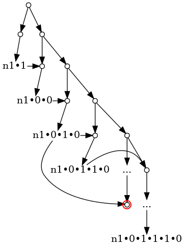
This can be seen in the visualization on the left side of
Figure 2, which is produced automatically by our
implementation from the inferred graph type.
In the figure, vertices in the graph, notated with either a text label or a
small circle, represent pieces of computation.
The vertices with labels like are the final vertices of
a future, and these labels are the vertex names assigned to the future.
The reason for these particular labels will become clear later in the paper.
Edges represent dependences: an edge out of a labeled vertex indicates a
touch of the corresponding future, and other edges represent sequential
dependences within a thread or the spawning of a future.
A path of edges in the graph therefore represents a chain of sequential
dependences and two vertices with no path between them indicate opportunities
for parallelism.
Long paths indicate a lack of parallelism.
The figure shows a visualization of the graph type of the program, with
the recursion of unrolled a fixed number of times to make
the recursive structure visually clear.
A vertex labeled indicates a recursive call that has been elided
because of the cutoff on number of unrollings.
The vertex representing the operation in
is circled in red: we can see that there is a long chain
of dependences on the critical path to reach this operation, which means the
operation will be significantly delayed when running the program.
Indeed, the topmost appears on the critical path, indicating a
potentially (and, in this case, actually) infinite critical path.
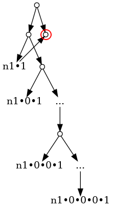
The second implementation in Figure 1 instead uses
a new data structure which resembles a lazy list: the head
of the list is computed eagerly and may be used immediately but the tail of
the list is computed asynchronously in a future.
The function takes the running total
(now as an actual float, rather than a future) and .
It adds the th approximation to the running total,
then returns the new running total as well as a future to
call recursively to compute the remainder of the pipeline.
This is reminiscent of the “producer” example of Blelloch and
Reid-Miller (1997).
As we can see from the visualization on the right side of
Figure 2, the graphs corresponding
to exhibit much more parallelism than the previous version.
Here, the operation in (again circled in red)
occurs in parallel with the computation of the remainder of the list
and there are only a small, finite number of operations on its critical path.
Figure 1. Two implementations of a function that iteratively computes
with futures.
In this paper, we present a graph type system that can statically compute graph
types for the above pipelining examples (and many more), thus allowing us to
detect and repair the parallelism bugs we discussed.
We present the type system in , a core calculus containing
both futures and recursive types.
The key to our approach is parameterizing recursive data structures involving
futures with a source of fresh vertex names called a vertex structure (or
VS, for short).
Conceptually, one can think of a VS as a separate structure of the same shape
as the program’s recursive data structure, containing unique vertex names.
For example, both the and the of
Figure 1 would be parameterized by a stream of vertices.
The two functions and would take this
vertex stream, let’s call it ,
as an implicit parameter and, at each iteration, use the next
vertex in the stream () to spawn the new future and pass the
rest of the stream () to the recursive call.
As a result, the returned list (resp., pipe) will be “zipped” together with
the vertex stream in the sense that the first future in the list (resp., pipe)
will use the first vertex of the stream, and so on.
In this way, we need not “unroll” the vertex structure at compile time:
the types will refer to projections of a VS parameter.222We do, however,
unroll a VS when unrolling the corresponding graph types, e.g., to create
the visualizations in Figure 2. In the figure,
is the “root” of a VS and the notations that follow are projections
of this VS.
Vertex structures are not limited to streams: in general, a VS can be an
infinite (corecursive) tree with arbitrary branching patterns.
We show that this allows us to construct a VS corresponding to
arbitrary recursive data structures.
Figure 2. Visualizations for list_pi (left) and pipeline_pi
(right) showing the differences in parallelization strategies. In both
figures, the node corresponding to the touch operation in
main is circled in red for emphasis.
Recall that we require vertex names to be unique.
The vertices contained by a vertex structure are all unique,
but ensuring that each vertex is used at most once is non-trivial
and requires numerous extensions to the graph type system.
One source of complexity is that types can perform significant computation
on vertex structures.
As an example, as we discussed above, the same vertex cannot be used as
a name for two futures.
In the presence of computation on VSs, this is not a simple restriction to
enforce syntactically: if is a vertex structure,
then under a reasonable semantics for
vertex structures, and refer
to the same vertex name and therefore cannot both be used to spawn futures.
The calculus assumes that data structures are annotated with
vertex structures and makes explicit many of the manipulations of VSs
described above.
However, should be seen as an intermediate representation—an
inference algorithm can infer all necessary annotations from unannotated code
in a high-level source language.
As a proof of concept, we extend GML (Muller, 2022), a graph type checker for
a subset of OCaml (but which did not previously support lists containing
futures, or any sort of user-defined algebraic data types) with support for
user-defined algebraic data types containing futures.
Our graph type checker is able to infer annotations and produce graph
types from the examples in Figure 1, as well as all of the
other examples contained in this paper, with no additional
annotations or programmer burden, as well as to produce visualizations of their
graph types.
As shown in the example above, such visualizations can allow programmers to
identify errors in the parallelization of their code, and can also be used
to reason about parallel complexity and other features.
Prior work (Muller, 2022) also explains how graph types can be used to
aid other analyses, such as deadlock detection.
A formal presentation of the inference algorithm is out of the scope of this
paper, but much of the challenge in our extension is constructing the
vertex structure corresponding to an arbitrary user-defined algebraic data
type.
We describe this process formally and prove some metatheoretic results about
it.
In sum, our contributions are:
•
, a parallel calculus with a graph type system
supporting recursive data types (Section 3).
•
A soundness result for , guaranteeing that the graph type of a
program correctly describes the computation graph that arises when running the
program (Section 4).
•
An algorithm for inferring the shape of a vertex structure that will
provide the necessary vertex names for an arbitrary recursive data structure,
and results showing (among other things) that such a VS exists for any
valid recursive data type (Section 5).
•
A prototype implementation of graph type inference for an OCaml-like
source language, including OCaml-style user-defined algebraic
data types mixed with futures (Section 6).
Technical details of the type system and many of the proofs are contained
in the appendix, which we reference throughout the paper.
We begin with an overview of graph types as well as a high-level description of
our extensions.
2. Overview
We begin with an overview of graph types but refer the interested reader to
the original paper (Muller, 2022) for a more thorough presentation; we
indicate using footnotes where we diverge from that paper’s presentation.
Our motivating example is a parallel implementation of Quicksort using
futures (Figure 3).
The code is supplemented with annotations in gray that are inserted during type
inference and used in the formal presentation of , but are not
written in actual code; these annotations will be explained later, in
Section 3.
The implementation returns immediately in the case of an empty list.
On a non-empty list, the first element is selected as a pivot and used to
partition the list using a sequential function , whose
implementation we omit.
A future is spawned to sort the first list recursively while the
second list is sorted in the main thread.
When the second list is sorted, we touch the future to retrieve the sorted
first list, and append the lists.
The type of the function in is given below the code; the type
indicates that accepts and returns an .
As is common in presentations of type-and-effect systems, we write an
annotation over the arrow indicating the effects performed by running the
function.
In this case, the “effect” is the graph type of the function; that is,
a graph type describing the family of computation graphs which might arise
from executing .
The prefix indicates that binds a recursive instance of
itself as —this notation is taken from standard presentations of
recursive types.
The body of is
a disjunction of two families of graphs, indicated by the symbol.
This notation appears when the code executes a conditional or pattern
match and indicates two possible families of graphs:
indicates that the graph can take a form indicated by either
or .
In the example,
the first graph type, , indicates a sequential computation
and corresponds to executing the base case.
The second graph type corresponds to the recursive case, and indicates that a
future is spawned.
In order to refer to this future later in the graph type, futures are assigned
unique names.
By convention, these names are assumed to refer to a vertex “attached” to the
computation graph of a future as a final vertex.
We will refer to this vertex as the “sink” vertex of the future,
borrowing a term from graph
theory because, until the future is touched, it has no outgoing edges.
The notation , which appears in
corresponding locations in the graph type and as an annotation in the
code, indicates binding a new vertex variable which locally refers
to a new, fresh vertex name; is the type of this variable and means
that refers to a single vertex.333This type annotation is not
used or needed in prior work, where only single vertices are bound. We
introduce it here for consistency with the syntax used in the rest of this
paper.
When the annotated program is evaluated (we do this only to prove soundness;
the vertex name annotations have no runtime meaning in the actual program)
or the graph type is unrolled (e.g., to produce the visualizations of
Figure 2), will be instantiated with a new,
fresh vertex name.444In the terminology of this paper, it will actually
be instantiated with a new vertex structure of type .
Figure 3. Code and types for parallel-recursive Quicksort using futures.
Code annotations
in gray are shown for convenience; these are not written by the
programmer.
The sequential composition of two graph types is
denoted , indicating that the program performs
a computation described by followed by one described by .
In our example graph type, the graph type corresponding to the recursive
case is the sequential composition of three operations.
The graph type indicates that is the sink
of a future whose graph is described by the graph type
(which, recall, is a recursive
instance of corresponding to a recursive call to ).
In general, indicates a future whose computation
graph can be described by and whose sink vertex is given the
name .
In , spawns using the keyword are also annotated
with the vertex that is used; this annotation is shown in gray in the code.
The spawn in the graph type
is then sequentially composed
with another instance of
for the other recursive call, and finally a touch of the future whose sink
is (a touch of vertex is denoted ).
Note that the vertex in the Quicksort example exists only within the
scope of the binding and so, in particular,
cannot be allowed to escape the scope.
If futures are, e.g., returned from a function, the vertices for those futures
must be created outside and passed as parameters to the function.
As an example, take the function in
Figure 4, which returns a future. This function is similar to
the analogous function of Section 1, but limited to two
approximations of .
The vertex parameter is made explicit in the annotations, and
also appears in the type of the function (shown on the
right side of the figure) as a binding.
This construct in a graph type binds two parameters.
Both parameters stand for vertex structures (VSs), type-level
(co)data structures containing vertices,
and both are annotated with vertex structure types
indicating their shapes.
The first parameter, , will contain the vertices the function may use to
spawn futures.
In the case of , it is annotated with VS
type , indicating a pair of vertices (recall
that is a VS type representing a single vertex).555Note that prior work had similar notation for
vertex parameters but, as it did not have vertex structures, allowed s to
bind arbitrary-length vectors of vertex parameters.
The introduction of vertex structures in the present work, which we will use
later to more substantial effect, also simplifies this notation and makes it
more uniform.
The second parameter contains the vertices the function may touch; in the
case of , it is empty as indicated by the unit VS
type .666The theory of does not include the
VS type to keep the calculus minimal, but it is included in our
implementation and would be a straightforward addition to the calculus.
The function returns a future (spawned using the first
component of the vertex structure ) that produces a pair of a float and
another future, spawned with the second component.
Note that the types of futures explicitly indicate the vertices with which
the future was spawned.
As in the Quicksort code, these vertices also appear as annotations on the
keyword which are inferred during type checking.
Finally, the graph type of the function body shows that the function
spawns a future using the vertex , which in turn spawns a future
using the vertex , which finally does not spawn further threads.
The code in Figure 4 also shows a function that calls
and touches the two futures.
The graph type of this function binds a new vertex structure for
the two futures, which no longer need to escape the function.
As in Quicksort, the new vertex structure is bound using a binding of the
form , where the vertex structure
type is now the product instead of .
The call to instantiating the bound vertex structure
variable with the new VS is indicated by substituting
for in .
Figure 4. A function that iteratively approximates
twice in a pipelined manner
Before proceeding, we make one additional note about the
graph type system.
We have referred to and similar as unique vertex
names—each vertex name can be used to spawn a future at most once,
otherwise the resulting graph will be ambiguous (if two futures have
as a sink vertex, there is no way to know to which future a
touch refers).
The graph type system (both ours and that of prior work) enforce this using
an affine type system that restricts the use of vertex names.
Figure 5. Code and types for a function that iteratively approximates
indefinitely in a pipelined manner.
Thus far, we have discussed examples that are within the capabilities of prior
work.
Now suppose we wish to generalize to continue producing
iterative approximations indefinitely.
The code in Figure 5 does this,
producing a value of type , also defined in the figure, which
is a recursive type containing an approximation and a future to
continue the pipeline.
This is reminiscent of the “producer” example of Blelloch and
Reid-Miller (1997), who
use futures in this general pattern to construct a wide variety of
pipelined data structures.
As in the Introduction, each iteration
computes the th term in the approximation, adds it to a
running total , and returns the new running total as well as a future to
call recursively to compute the st term.
Useful instances of the recursive data type cannot be typed with
the existing graph type system, because doing so would require an infinite
sequence of new vertex names and a way of associating each future in the
pipeline with successive vertex names.
One (incorrect but illustrative) approach would be to instantiate each future
in the type with a fresh vertex name using, for example, an existential.
The pipe type would then be annotated as follows:
This is still not useful, however, because it doesn’t allow any vertex name
to escape the scope of the single future type, just as the vertex in
the function was confined to the function.
The type tells us that the
future is spawned with some vertex, but gives no information about
which, an untenable loss of precision when we try to touch this future
and add an edge to its vertex.
As an illustration of this loss of precision, consider the following program,
and suppose we wish to use its graph type to check for deadlocks (simply put,
a program may deadlock if its graph type can unroll to a cyclic graph):
Each future in the list contains a function that touches the following
future in the list.
This is a fairly clear structure and a
visualization or suitable analysis of the graph type produced by our
system could show that the program is deadlock-free.
However, if the type of the output list were given as
,
the most precise thing that could be said about this list
is that it is a list of thunks under futures, each of which touches
any future in the list (or, indeed, without further information, any
future in the program), including itself.
Thus, a sound deadlock
detector would have to conclude that the program might deadlock.
As a more precise solution to the problem of generating unique vertex names
for elements in a data structure,
we introduce vertex structures, mentioned above, which we
allow to be (co)recursive and thus serve as the source or collection of vertex
names we need.
In the code annotations and the type of on the right side
of the figure, the function takes a vertex structure parameter of vertex
structure type , which is defined in the lower right side of
the figure to be a corecursive type of an infinite list or stream of vertices.
The return type of the function is , where the
recursive type is now parameterized by a vertex structure.
This vertex structure is threaded through the recursive structure of the
pipeline data type such that successive futures in the data type are associated
with corresponding vertices from .
The details of this are technical and so we defer them, as well as the formal
presentation of recursive data types in , to the next section.
As in , the first future
uses the vertex , which appears as an annotation in
the code and on the graph type ( contains ,
indicating a spawn of ).777We treat
corecursive vertex structure types as equi(co)recursive, so no unrolling is
needed.
However, now the function calls itself recursively to generate
the rest of the pipeline.
Because the function takes a vertex parameter, this recursive call must
instantiate the vertex parameter with a , and it does so with
the tail of the stream, .
This appears in the graph type
as .
We complete this overview with a demonstration of how the pipeline can be
consumed, which shows how vertex structures link individual futures to their
touches.
The function in Figure 5 consumes a pipeline recursively,
returning the value.
It also takes a parameter of vertex structure type , but
this time as the second parameter, because the function uses these vertices
to touch futures and does not spawn futures.
The use of as the parameter to the data type indicates that
vertices for futures in the pipeline will be drawn from the stream ,
which is enough information to infer in the graph type that the
touch targets the first vertex of .
The function then calls itself recursively with the tail of the vertex stream,
which also appears in the recursive instantiation of in the graph
type.
Finally, calls with the pipeline.
As we have seen before, the vertex structure is bound here so that its
scope covers its uses both for spawns (in ) and for
touches (in ).
The calls to both functions instantiate the vertex structure parameter with
the same vertex structure , linking the spawns and touches in the
graph types.
The graph type for composes the graph types of the producer and the
consumer and links the spawns and touches by instantiating both graph types
with the same vertex structure.
3. Graph Types with Vertex Structures
Figure 6. Syntax of .
This section provides a formal presentation of , whose syntax
is given in Figure 6.
In the remainder of this section, we describe the features of the language
in detail, focusing on the main novelties of compared to prior
work: vertex structures (VSs) and recursive types.
3.1. Vertex Structures and Their Types
Vertex Structures () contain vertices that represent futures in
computation graphs. As shown in Figure 6, VSs appear in
annotations within expressions, type constructors, and graph types;
these annotations are not inserted into real code by programmers, but
are filled in during type inference.
Vertex structures are classified with VS types (). The
VS type represents a single vertex, and only VSs of type can be used
to name futures. The product type
represents pairs of VSs in
and . The availability annotations and
indicate whether the corresponding component is available () or
unavailable () for spawning new futures; their use is
inspired by record types in the Cogent language (O’Connor et al., 2021).
The need for availability will become clearer later, when we
discuss the type system. Finally, we can also form
corecursive VS types , which we will use to generate
graph types that require a potentially unbounded number of vertices.
Figure 7 presents the rules for assigning VS types
to VSs. The judgment
denotes that the VS has VS type
, where and are contexts that map VS variables to
their types.
Vertices, and thus VSs, are treated in an affine manner to ensure that any
vertex is used at most once to spawn a future—this affine treatment leads
to the use of two contexts.
The first, , is an affine context storing vertices that may be used
to spawn futures and the second, , is an unrestricted context for
vertices that may be used to touch futures (we may touch a vertex any number
of times).
Because we wish to be able
to touch any vertex we spawn, the set of variables in will always be a
subset of that in .
A VS variable is well-typed if it is in either or , and
we assume that does not contain multiple
mappings for the same variable.
VSs can be variables (),888
Unlike the original
presentation (Muller, 2022), refers to a variable instead of a
vertex. pairs, and
projections. As seen in the rules U:Fst and U:Snd,
only available components can be projected. For example, if has VS type
, then is safe to
use, but is not.
Rule U:Subtype is a subsumption rule for the subtyping
relation on VS types, denoted and defined
in Figure 8.
We allow three forms of subtyping: first (UT:Corec1 and
UT:Corec2), we can freely roll and unroll corecursive VS types.
Second
(UT:ProdLeft and UT:ProdRight),
it is safe to take an available component and treat it as unavailable.
Third, the types of
unavailable components of VSs may be changed at will, which is safe since those
sides can never be used.
The VS typing rule U:Pair uses an auxiliary splitting relation
(O’Connor et al., 2021), which is
described in Figure 10.
This relation is responsible for
enforcing the affine treatment of contexts. The judgment
states that splits into the
disjoint contexts and . It is important that
and be disjoint so that futures spawned under and under
have distinct vertices. However, we allow a variable with a product
VS type to appear in both contexts, as long as the availability of the products is
in turn split between the two. This is allowed by OM:VarTypeSplit:
may split to
and if
holds. Intuitively, , ,
and are the same types but with different availabilities: if a
component of a product VS type is available in , then that component is
available in or or neither, but not both. For example,
if appears
in , we may
have in
and in ,
but we cannot have
appear in either and .
The VS type splitting judgment is defined in
Figure 9. The core mechanism of VS type splitting is
US:Prod, which states a VS type
may split into and
. Most of the other rules are
“search” rules allowing applications of US:Prod in nested VS types. The
other significant VS type splitting rule is US:Subtype, which allows for
“weakening” the VS types resulting from a split (by turning available sides of
product VS types to unavailable).
3.2. Graph Types and Type Constructors
(DW:Spawn)(DW:Touch)(DW:New)(DW:RecPi)(DW:App)
Figure 11. Selected rules for graph type formation.
There are two kinding judgments to
characterize well-formed types: one for graph
types, and another one for type constructors.
For graph types, the judgment
states that the graph type
has graph kind
(Figure 11).
The context maps graph type variables to their kinds, and is
used to check that recursive graph types are well-formed
(see DW:RecPi).
The full set of graph type formation rules are given in Figure 32 in the appendix.
For type constructors, the judgment
states that the type
constructor is well-formed and has kind (Figure 12).
The context maps type
variables to their kinds.
Type constructors can be ordinary types, which are given the kind
(and for which we sometimes use the metavariable ).
Types may also be parameterized by vertex structures.
This allows, for example, a type of lists of futures which is parameterized
by the VS providing the vertices for the futures.999We could use the
same type parameter mechanism to allow types to be parameterized by other
types, as in the ML type ’a list, but this is orthogonal and we
do not consider it in the formalism to streamline the presentation.
The kind classifies
type-level functions that take a VS of type and return a type
constructor of kind . Rule K:Lambda describes how to
assign the kind to such functions.
As mentioned earlier, the motivation behind is to allow
recursive types containing futures. We achieve this by
parameterizing recursive types by VSs containing the vertices for these
futures. The syntax for a parameterized recursive data type is
, where
is a type level VS function (equivalent to
), is a recursive binding of
, and is the argument applied to
when the recursive type is unrolled. The formation
of parameterized recursive types is performed by K:Rec, in which
has kind within since it
represents a type-level function that passes a VS argument to the VS argument of
the recursive instance (seen in more detail below). By applying a sub-VS of to an instance of
in , the type
is able to recur over
. (Note that non-parameterized recursive types do not require special
syntax because we can parameterize them in a trivial way by using a dummy VS as
the parameter.) We can now implement the type constructor for a list of integer
futures as
(UE:FstPair)(UE:SndPair)
Figure 13. Selected rules for vertex structure equivalence.
(CE:Fut)(CE:BetaEq)
Figure 14. Selected rules for type constructor equivalence.
Because VSs can occur in types, type checking programs may require
performing some type-level computation, notably when projecting vertices out of
a VS. To address this, we introduce two judgments: an equivalence judgment on
VSs, (see Figure 13), and an equivalence
judgment on type constructors,
(see Figure 14). Regarding VSs, the most notable
rules are UE:FstPair and UE:SndPair, which
extract (available) components of a pair.
For type constructors, equivalence has two
purposes: performing a type-level VS function application, which is performed by
CE:BetaEq; and changing VSs within types to equivalent VSs according
to the VS equivalence rules (CE:Future is given as an example).
The full set of VS equivalence and type equivalence rules are given in Figures 33 and
34 respectively in the appendix.
Figure 15 presents the type system for , which assigns
graph types (and types) to expressions. The judgment
states that the
expression has type and graph type . In addition to the
graph type context and
VS contexts and , this judgment uses the
context which, as usual, maps expression variables to their types.
We give a quick overview of the graph type system: represents
expressions that execute purely sequentially;
represents expressions that execute an expression with graph type
followed by an expression with graph type ;
represents expressions that execute an
expression with graph type or an expression with graph type
; is a recursive graph type;
represents spawning a future at vertex that
executes an expression with graph type in parallel;
and represents touching the future at vertex .
A parameterized graph type
accepts two VSs as arguments ( has VS type
and is added to and while has VS type
and is only added to ).
Such graph type functions are applied
with the syntax .
Finally, binds a new
VS variable of VS type and represents expressions that do the same.
Rule S:Fun types function expressions
where is the name of the function,
is an expression parameter, and are two VS parameters, and
is the body of the function. Excluding bindings of new VS variables within
, the only VS variable that can be used for spawning futures in is
, while future touches can use any VS variable within the context
(including and ), hence the function having two VS
parameters. The type of functions is
where is the type of the
parameter , is the type of the function body, is the graph
type of the function body, and
is the graph type representing graphs produced by applying the function. The
function type is parameterized by the VS parameters and (the same
ones from the function expression), which have VS types and
respectively. The graph type
contains a recursive binding to a graph type function whose body is
(note that this function binds a new, separate and within
), and this recursive binding is applied to the and
bound within the type. This allows to pass different VS arguments to
recursive instances of itself (this is useful, for example, when recursive
instances access deeper levels of a vertex stream). In addition to adding the
function expression’s parameters to the context when typing the function body, we add , the
recursive binding of the function; and , the recursive binding of the
graph type function whose body is .
Rule S:Type-Eq ensures that typing respects type
constructor equivalence.
Rules S:Roll and
S:Unroll roll and unroll parameterized recursive data types:
unrolls to
by applying to (hence
) and then substituting itself recursively. Instead of
replacing the with an instance of the recursive type, we replace it
with a type-level VS function that passes its argument to the recursive type.
4. Soundness
The goal of this section is to prove the soundness of the graph type system
for ; that is, that the computation graph of a program is described
by its graph type.
In order to prove this theorem, we must first formalize 1) the notion of a computation graph being “described by” a graph type
and 2) the operational
semantics by which a program evaluates to produce a computation graph.
The first notion is one of normalization (Muller, 2022), a process
for constructing the set of computation graphs corresponding to a given
graph type.
The second is a cost semantics, which we present as a big-step semantics
that evaluates an expression to a value and a computation graph.
The rest of this section is structured as follows.
In Section 4.1, we discuss how we represent the
creation of new vertices (which occurs during both normalization, as
bindings are normalized, and during evaluation, as they are evaluated).
We then formalize normalization (Section 4.2), and
finally present the cost semantics and prove soundness
(Section 4.3).
Figure 16. Selected rules for vertex structure normalization.
Recall that the constructs in graph
types and in expressions
bind “fresh” vertex structure (VS) variables to be used in the graph type
and the
expression, respectively.
Because VSs can be infinite and of arbitrary type,
some care must be taken in how to represent them at
“runtime”, i.e., in normalization
and the cost semantics.
The key insight is that VSs
are (possibly infinite) trees with unique vertices at each leaf.
It is thus possible to uniquely identify a vertex by the VS it
comes from, and the path taken to reach it from the root of the VS.
Paths in a vertex structure are already represented in our syntax
as sequences of projections, e.g., , so most of the
new conceptual work is in representing the roots of the vertex structures.
We use the syntax and variants to represent a unique vertex
name, called a generator,
which serves as the root of a VS .
Generators are included in the contexts and like VS
variables, but are meaningful runtime symbols representing unique
VSs.
We will use the notation and to refer to contexts that
contain only generators, and no variables.
These are the only contexts that will exist at runtime for typing top-level
terms and graph types, as such terms and graph types contain no free variables.
We refer to these terms and graph types as closed
even though they may contain free vertex names in
the form of generators.
The judgments for VS typing and context splitting are extended with
rules for generators that resemble the rules for variables.
Equipped with a way to represent the roots of new vertex structures, we turn
our attention again to paths from the root to a vertex.
Currently, the same path can be represented in multiple ways,
for example .
It will be useful to have a normal form for paths,
so we introduce a normalization operation on VSs with the
judgment , defined in
Figure 16 (rules symmetric to these are omitted).
Intuitively, the operation -reduces any projections of pairs (but
leaves alone projections of vertex structures that are not syntactically
pairs, e.g. ).
Figure 17. Extended syntax for generators, vertex paths, and values
(S:Handle)
Figure 18. Rule for typing handles.
We use the term vertex paths, and the notation ,
to refer to closed, normal VSs.
Figure 17 extends the syntax for VSs with generators and
gives the syntax for vertex paths.
We now have a way of producing references to unique vertices: generators give
rise to unique, non-intersecting VSs, and unique vertex paths in
a given VS refer to unique vertices.
When evaluating a binding, we will simply create a fresh generator.
The remainder of the vertices in the VS are then created
implicitly, and will be accessed by the program as it traverses the VS.
4.2. Normalization
(UR:Seq1)(UR:Seq2)(UR:Rec)
Figure 19. Selected rules for graph type unrolling.
Figure 20. New- normal form.
Figure 21. Graph type expansion.
Figures 19–21 present the machinery for
normalization.
Because a recursive graph type represents an infinite set of graphs (as it
can be unrolled any number of times), we stage the construction of these sets
so that every set constructed is finite.
Constructing a set of graphs consists of three operations, each of which
performs some of the required tasks.
First, recursive graph types are unrolled a desired number of times,
yielding another graph type that is equivalent up to unrollings of
recursive bindings.
Next, the graph type is reduced to “New- normal form” (NBNF),
which “evaluates” any exposed “new” bindings by generating and substituting
fresh vertex structures.
This process also performs any applicable reductions on exposed
applications.
At this point, we are left with a valid graph type, but one with no exposed
“new” bindings or applications.
Finally, the resulting graph type is expanded into the set of graphs;
because there are no exposed “new” bindings, this process does not involve
generating any new vertex names or structures.
We will now discuss each of these steps in more detail.
Figure 19 gives a small-step semantics for unrolling
recursive bindings in graph types.
The bulk of the work is done by rule UR:Rec, which steps
a binding to .
The remaining rules “search” the graph type for recursive bindings, so
we defer the full set of rules to Figure 38 in the appendix.
Note that, unlike in a standard left-to-right (or right-to-left) operational
semantics, the rules UR:Seq1 and UR:Seq2 allow any
instance of recursion in the type to be unrolled at any time in a
nondeterministic fashion.
For example, both steps below are valid:
The rules for reducing to NBNF, given in Figure 20,
eliminate “new” bindings by substituting fresh vertex structure generators,
and perform any exposed applications.
Evaluation proceeds recursively through sequential compositions
and alternatives, but not under binders.
As a result, closed sub-graph-types of NBNF graph types are themselves NBNF.
Finally, Figure 21 gives the rules for expanding a graph
type into the set of graphs it represents.
We represent a graph
formally as a 4-tuple
containing the sets of vertices and edges , as well as
a designated “start” vertex and “end” vertex .
We use shorthands for combining graphs sequentially and in parallel; these
shorthands use many of the same operators as graph type composition, but
should not be confused.
Figure 22 gives formal definitions for these shorthands; for more
description of them, the reader is referred to prior work (Muller, 2022).
In brief, sequential composition joins the end vertex of the first
graph to the start vertex of the second graph.
The “left composition” operator (Spoonhower, 2009),
written , adds a subgraph
corresponding to a future to the graph, with an edge representing the spawn.
It also adds the vertex as the sink of the future’s graph.
The “touch” operator adds an edge from .
Figure 22. Shorthands for combining graphs.
Sequential compositions are expanded by expanding both
subgraphs, and then sequentially composing the resulting graphs.
Alternation simply takes the union of the two sets of graphs.
Expansion does not perform any additional unrolling, so the expansion of
a recursive graph type is the empty set of graphs.
Expansion of the future
is performed by left-composing all of the resulting graphs with the
vertex , and touches simply expand to the singleton
graph consisting of the touch.
Note that because NBNF has already expanded all “new” bindings,
there is no rule for expanding these, and
expansion does not generate new vertex names.
The latter is a key property in guaranteeing that expansion results in
well-formed graphs.
These three operations combine to form a normalization process that is correct:
any set of graphs that results from unrolling, normalizing, and expanding a
well-formed graph type is well-formed. This result is formalized by Theorem 1,
which is proven in Appendix B alongside several necessary technical lemmas in Appendices A and B.
Theorem 1.
If
and ,
then exists and if ,
then is a well-formed graph.
4.3. Cost Semantics and Soundness
We equip with a cost semantics,
a big-step operational semantics that evaluates an expression and also produces
the computation graph that represents the execution.
The judgment is , meaning that expression
evaluates to value , producing the cost graph .
The rules for this judgment are in Figure 23,
and the syntax for values are in Figure 17.
In C:Future, the body of the future is evaluated (in a real
execution, the body of the future will be evaluated in parallel, but the
big-step cost semantics deliberately abstracts away evaluation order)
and the future evaluates to a handle, a new syntactic form which records the
result of the future.
In addition, we evaluate the vertex structure used to spawn the future
to a vertex path , which is recorded by the handle.
The C:Touch rule extracts both the vertex path and future result
from the handle.
In C:New, a new generator is created and used to
generate a vertex structure which instantiates the variable .
Figure 23. Cost Semantics for (selected).
Rules symmetric to these are omitted.
The soundness theorem for the graph type system of is that
if a program has a graph type and evaluates to produce
a graph , then is described by (that is,
should be in the set of graphs obtained by
normalizing using the machinery in the previous subsection).
This is stated formally as Theorem 2.
The formal statement of the theorem also includes a context containing
generators created during execution which may be captured in the result
value .
Theorem 2.
If
and ,
then there exists a
such that implies
and
and there exists a such that
and .
The proof of the theorem can be found in Appendix B
alongside several necessary technical lemmas in Appendices A and B.
5. Elaboration of Recursive Types with Vertex Structures
Thus far, we have presented the annotated language containing
recursive data types ,
annotated with a vertex path of type that provides
vertex names for data structures of the recursive type.
We have motivated that should have a structure that in some sense
“maps on” to the recursive structure of the list so that any futures in
the structure have a corresponding vertex name.
As examples, a list data type corresponds to an infinite stream of vertices,
and a binary tree data type corresponds to an infinite binary tree of vertices.
As discussed, the annotated language is provided merely as a core calculus
for expressing the ideas of the graph type system; the annotations can be
inferred from unannotated code by our implementation.
Other than the addition of vertex structures, the general structure of the
algorithm for inferring these annotations is similar to that of
GML (Muller, 2022), and the details of the algorithm are largely outside the
scope of this paper.
However, one important and non-obvious fact for inferring annotations
for is that it is indeed possible to annotate any recursive
data structure with a corresponding vertex path.
Showing this fact is the goal of this section.
We do so by defining a set of rules for annotating unannotated types and
values with vertex structure annotations.
For simplicity, the system we present in this section is declarative and not
algorithmic, so it still abstracts away many of the complexities of our
inference algorithm, but we show that the rules are complete and thus that any
recursive type may be so annotated.
We first define a syntax for unannotated types and
unannotated values .
Unannotated types consist of the unit type, functions, products, and sums,
as well as an unannotated future type and an unannotated recursive type.
Note that the annotation of functions is orthogonal to the annotation of
recursive data types; we assume that function types and function values have
already been annotated and include annotated function types and annotated
function values as unannotated types and unannotated values, respectively.
The unannotated future type is similar to the annotated
future type but is not annotated with a VS.
Similarly, the unannotated recursive type
binds a type variable but does not bind a VS variable and
does not take a VS as an argument.
Because unannotated types do not interact with vertex structures, there is
no type-level lambda and all unannotated types have kind (and so
we do not distinguish between “unannotated types” and “unannotated type
constructors”).
Unannotated values differ from values only in that future handles are
not annotated with vertex paths.
Figure 24 defines the
judgment .
This indicates that may be annotated to the type constructor
(which will, by construction, have kind ).
It also returns a vertex structure type that “corresponds” to the
type .
For recursive types , the VS type is the
type of the VS annotation for the recursive type (that is,
will be annotated to be
for some and some ).
As an example, if is the type of int future
lists,
then will be (equivalent to) the type of vertex
streams, .
The judgment takes a type variable context mapping type variables
to kinds (these will be annotated types and so their kinds will not be ).
It is also parameterized by a vertex structure to use for annotations.
When annotating a closed unannotated type , this parameter will
simply be instantiated with a fresh vertex path to
derive .
The returned type would be annotated with projections of .
The returned VS type would be the type that
should be assigned in order for to be well-kinded.
Rule F:TyVar looks up the type variable in the context.
By construction, its kind will be of the form ,
indicating that to properly annotate the use of the variable ,
it must be applied to a VS of type .
We use the VS for the annotation and return the
type as the required type of .
The unit and function types do not require additional annotations, and so
are simply returned.101010The returned VS type is ,
which will result in the
addition of unnecessary vertices to the final VS; it would
be straightforward to add a multiplicative unit to VS types,
which would be the most appropriate VS type to return here, but
we have not done so this far to keep the VS type language as
simple as possible.
Rule F:Prod takes a VS and annotates
the first component with the left projection of
and the second component with the right projection.
The type required for is thus the product of the two returned types.
Rule F:Sum, somewhat counterintuitively, also returns a product
of the two VS types.
This is because if a data structure can take one of two forms, the
corresponding VS must offer either
possibility.111111As an optimization, we could take a “maximum” over the
two VS types. For example, in a 2-3 tree, where each node
may have two or three children, the corresponding VS could
always offer three branches and a 2-node would use the first two.
Rule F:Fut takes to be a product whose second component
is a single vertex, which it uses to annotate the
future; the first component is used to annotate the future’s return type.
Finally, rule F:Rec annotates a recursive
type .
It begins by adding to the context with
kind
(this is the only truly non-algorithmic feature of these rules;
we do not discuss how to construct ).
With this context, it annotates .
The resulting VS type is rolled back into the corecursive
type , which is the type required for .
Example.
We can represent the type of a list of integer futures as an unannotated
type :
Using the rules of Figure 24,
we can infer the following annotation for :
where .
The VS corresponding to is a stream of vertices
(note that because we treat VS types equi-corecursively, the VS type above is
equivalent to
but unrolled slightly).
In the body of the recursive annotated type, which is
,
the first vertex of the stream is discarded (this is an effect of mapping the
type to the VS type even though it does not need a vertex),
the second vertex of the stream (the first vertex of the tail) is used for the
future and the remainder (the tail of the tail) is passed to the recursive
instance of the type.
Figure 24. Annotating types with vertex structures.
The judgment described above declaratively shows a correspondence between
unannotated types and the vertex structure types required to annotate them.
Later in this section, we show that this relation is complete with respect to
well-kinded unannotated types, and thus that any type has a corresponding
VS type.
We next wish to show that a VS of the returned VS type actually
does suffice to provide all necessary vertices for a data structure of the
given type.
We do this using another judgment that annotates unannotated values.
This judgment is defined in Figure 25
and takes the form ,
where is a vertex path to use for annotation (similar to the type
annotation judgment above), is an unannotated value, and
is the annotated value.
We restrict annotations of values to vertex paths since the value may only use vertex paths as the handle.
Otherwise, annotation of values proceeds in much the same way as annotation of types.
Rule FE:Pair uses the two components of
to annotate the components of the pair.
Rules FE:InL and FE:InR use the first
and second components, respectively, of to annotate left and right
injections (recall that, for a sum type, is given a product
type so that the two components of may be used for the two
injections).
Finally, just as F:Fut uses the first component of
to annotate the type of the future’s payload and the second component as the
vertex for the future, rule FE:Handle uses to
annotate the payload and to annotate the handle itself.
Figure 25. Annotating values with vertex structures.
Example.
Consider the list of integer futures from above.
We claimed that the correct VS type for this type
is .
The rules of Figure 25 provide a “recipe” for
constructing a future list using a vertex path of VS type .
As an example, consider the unannotated value
which represents the list containing two future handles, one returning 1 and
the other returning 2.
Applying the rules, we get the expression
As described above, the futures take
consecutive odd vertices from the stream .
The main result of this section has three components.
First, any well-kinded unannotated type may be matched with an annotated type
by the rules of Figure 24.
Second, if a well-kinded unannotated type is annotated with a VS of the VS type
returned by the annotation judgment, then the annotated type is also well-kinded.
Third, if an unannotated type is annotated with a vertex path
(that is, if ),
then any well-typed unannotated value of type
may be annotated with by the rules of Figure 25,
and the annotated value is well-typed when has type .
Moreover, to show that has “enough” vertices to fully
annotate the value with unique vertices, we show that the annotated value
is well-typed under a new typing judgment that uses only an affine context
for vertices.
Usually, values would be typed with the unrestricted
context , because a data structure is allowed to contain multiple
handles to the same future, but in this case, we wish to show that we
can restrict data structures to use new vertices for each handle.
We write the new judgment .
The rules are similar to the standard
typing rules, but use the affine context for typing handles.
This rule for typing handle values
is given in Figure 27.
Values always have the graph type , so we omit the graph
type from the judgment.
The full set of affine typing rules for values is given in Figure 39 in the appendix.
(SV:Handle)
Figure 26. Affine typing rule for handle values.
Figure 27. Annotating and unannotating kinds in .
Theorem 1 formalizes the main result of this section,
that is, that 1) type annotation is complete with respect to well-kinded
unannotated types, 2) type annotation annotates well-kinded unannotated types
into well-kinded types, and 3) annotating values with vertex structures of the
returned VS type results in well-typed values.
In order to show this, we introduce a kinding judgment for unannotated types,
,
and a typing judgment for unannotated values, .
The rules for these judgments are similar to those for annotated types
and expressions and can be found in Figures 40 and
41 of the appendix, respectively.
Since the kinds of type variables
bound by unannotated and annotated recursive types are different
( and respectively),
we need some way to change the kinds that these type variables are bound to.
We address this with the functions and .
takes a context suitable for annotating types
and kinding annotated types
(where type variables can, and will always,
have kind ),
and return an unannotated context,
one suitable for kinding unannotated types
(where every type variable has kind ).
performs this process in reverse, where the VS type
expected by every type variable in is a fresh VS type variable
unique to that type variable (each which can be substituted with the desired VS type).
The proof of Theorem 1, as well as statements and proofs of several
necessary technical lemmas, appears in Appendix C.
Theorem 1.
(1)
For an unannotated context ,
if ,
then for any ,
there exist and
such that .
(2)
If
and
and ,
then .
(3)
If
and
and ,
then there exists such that
and for any such that .
we have .
6. Implementation and Examples
We have implemented a prototype graph inference algorithm for on top
of GML (Muller, 2022), an existing graph type inference algorithm.
The goal of the implementation, which we call GMLμ,
is to infer vertex structure annotations
and graph types from ordinary, unannotated OCaml programs.
GML extends OCaml syntax with the keywords for
spawning
expressions into a future, for joining a future handle’s value to
the current thread, and a type .
Additionally, GMLμ supports OCaml’s user-definable recursive datatypes,
which were not previously supported by GML (there are some limitations,
which we discuss at the end of this section).
For example, we can define the type from
Sections 1 and 2
using standard OCaml syntax:
Our extension of GML successfully infers the corresponding vertex
structure annotations, for the type itself and for all of its uses in the
code in Figure 5.
In addition, we implemented (by extending facilities existing in GML)
a visualizer that uses several heuristics to generate a visualization of
a representative graph corresponding to each inferred
graph type.121212Once the graph type is unrolled to generate the
representative graph, we output a file that can be turned into a visualization
using GraphViz (Gansner and North, 2000).
This allows developers to see at a glance how their program will parallelize.
We have used GMLμ to infer graph types
for all example programs in this paper.
The details of the implementation are out of the scope of the paper.
However, the main challenge in extending GML with support for algebraic data
types is generating the VS type corresponding to an ADT.
Our algorithm for this closely follows the presentation of
Section 5.131313As discussed in that section, the only
non-algorithmic
detail of the presentation was constructing in F:Rec;
in the implementation, we add
to the context instead of .
This means the context contains non-well-formed VS types, which makes the
theory more unwieldy but yields a convenient implementation.
When processing a type declaration, GML generates the associated
VS type, and also generates a constructor and deconstructor function for
each constructor.
Constructor applications are desugared to ordinary applications of the
constructor function and the deconstructor function is used during pattern
matching.
Another major challenge is implementing unification on vertex structures.
At the moment, our implementation uses a set of heuristics that are not
guaranteed to be complete (i.e., unification may fail for VSs that could be
unified, resulting in a spurious type error) but work well in practice on the
large examples tested.
In addition to extending the subset of OCaml supported by GML, we
have also substantially re-architected the code.
In GMLμ,
the graph type checker is completely separate from the type checker.
This simplifies the implementation and has a number of other benefits.
First, all futures in a program are known by the time graph checking begins.
This allows the implementation to infer graph types in several instances
where type annotations would previously have been required
(one such instance is noted in prior work (Muller, 2022) as a limitation
of GML,
which is not a limitation of GMLμ).
Additionally, this architecture would simplify the process of integrating
graph checking as an extension of the OCaml compiler, as an additional pass
on type-checked ASTs.
6.1. Examples
To show the utility of GMLμ, we discuss several example programs
for which it can infer and visualize graph types.
Produce-consume
The producer-consumer example of Blelloch and
Reid-Miller (1997), shown in
Figure 28,
is similar to the function of Figure 5,
but allows the pipelined list to be finite (ending with ).
As in the pipeline example, the constructor allows the
tail of the to continue being computed in a future.
We compose , which (for the sake of a simple example)
outputs a list of the numbers 1–n,
with the function which calculates the sum of the list.
In the graph of the composed functions (right side of the figure), the
touches of happen in parallel with the production of
the list.
Figure 28. Blelloch-Reid-Miller produce-consume example
Tree Sum
In Figure 29, we present operations
on a pipelined tree data structure (Blelloch and
Reid-Miller, 1997).
As with , the two subtrees of an are futures, so they may be computed asynchronously while the value at the node is used.
The function
generates a tree of numbers 0 to 10, then
calculates the sum of elements in the generated tree.
While the particular application of summing a binary tree is fairly simple,
one can imagine using the same structure for more complicated use-cases.
Because of the design of the data structure,
immediately returns a future and then
can perform its calculation as later recursive steps of
are still executing.
The function in Figure 30 reverses a pipelined tree of
the type defined in Figure 29.
Here, the interesting feature of the output was not the visualization of the
function’s graph type, which shows a similar structure to
and , but the function type, which is
where .
We omit the graph type for clarity.
The function takes two VS parameters and a tree indexed by and
returns a tree indexed by .
At first glance, this may seem imprecise because one might expect the VSs
parameterizing the input and output tree to be related (after all, the output
tree is the reverse of the input).
However, this is not correct:
touches (in a pipelined way) all of the
futures of the input tree and constructs a new tree with the reversed
values but new futures from the VS .
Here, not just the graph type but the return type parameterized by its VS
can correct a misunderstanding about the parallel behavior of a program.
6.2. Limitations
Though our inference algorithm checks most useful programs, there are some limitations.
First, polymorphic types cannot be instantiated with types
that include futures.
For example, a list of futures would have to be explicitly defined as a
new type rather than by instantiating built-in lists
to form the type .
This represents a design trade-off; graph types are not currently expressive
enough to represent, say, a function on lists of futures.
If the standard list type could be instantiated with a
future, the polymorphic function would need to be
assigned a general enough type to cover all instantiations of ,
which wouldn’t be possible.
A limitation we inherit from GML is that functional arguments
of higher order functions
cannot spawn futures.
This is possible in , but cannot be inferred without annotations.
7. Related Work
Graph Types and Related Analyses.
The use of graphs to represent the parallel programs dates back
to at least the late 1960s (Karp and Miller, 1966; Rodriguez Bezos, 1969).
Our notation is most directly inspired by the work
of Blelloch and
Greiner (1995, 1996) and Spoonhower (2009), who extended
these graphs with notations for futures.
In this work, graphs were produced dynamically from programs using a cost semantics, which abstractly evaluates the program to form the graph
(or a family of graphs if execution is nondeterministically).
The first work we are aware of on statically approximating such graphs for
fine-grained parallel programs was the prior work of
one of us (Muller, 2022), which developed
a calculus and corresponding graph type system for inferring
graph types of parallel programs with futures.
Our work builds on , including the use of an affine type system
to ensure that vertex names are unique and therefore do not appear twice
in a graph, which would result in an invalid graph.
However, the main thrust of this paper is overcoming the significant limitation
in that affine treatment of vertex names prevents building
collections of futures.
Dependency graphs are frequently used to represent
control dependencies in coarse-grained parallel programs and these have been
the target of several static analyses
(e.g., (Chen
et al., 2002; Cheng, 1993; Kasahara et al., 1995)) but such tools do
not contend with the substantial dynamicity inherent in fine-grained parallel
programs, especially those with futures.
Dependency graphs are also used to represent other dependencies in a program,
including data dependencies; analyzing the structure of such dependencies is
a form of program slicing (e.g., (Weiser, 1984; Korel, 1987)).
As observed in prior work (Muller, 2022), graph type systems draw on ideas from
region type systems (Tofte and Talpin, 1997), where assigning a vertex to
a future corresponds to allocating an object within a region of memory,
in order to
aid in memory management and/or ensure safety (e.g. (Fluet
et al., 2006)),
including in the presence of concurrency and complex, dynamic
data structures (Milano
et al., 2022).
It is not possible to list all of the
related work on regions and related systems, so we refer the interested reader
to the chapter by Henglein
et al. (2005).
Two major differences with region systems are that vertex assignments must
be unique (whereas typically many objects are allocated within a single
region) and that, to generate useful graphs, we wish for vertex assignments
to be visible at a global scope (see the example from the Introduction of
why locally allocated vertices are not suitable for graph types of data
structures).
Heterogeneous and Indexed Data Structures.
Indexed types (Zenger, 1997; Xi and Pfenning, 1999), a limited form of dependent types
in which a type is indexed by a value from a specified domain,
have long been used to add expressiveness to types—a classic example is a
type of vectors indexed with a natural number giving the vector’s length.
We index recursive data types with a vertex structure
to assign unique vertices to futures in recursive data structures.
Vertex structures have a non-trivial semantics of their own but are not
first-class objects at the expression level, so computation on VSs
may be seen as an instance of type-level computation.
A similar indexing idea and type-level computation have been previously
combined to achieve heterogeneity in HList (Kiselyov
et al., 2004), a Haskell
library that expresses heterogeneous lists by indexing the list type
constructor with a type-level list.
Their work does not appear to generalize beyond lists or to infinite indices.
Richer forms of type-level computation have been explored, and could be used
to further generalize the theory of vertex structures.
Yorgey et al. (2012) extend Haskell’s kind system with features for
expressing a variety of type-level data structures.
As another example, we have considered extending vertex structures
with sums (so a vertex structure could, e.g., represent a
finite list) and using type-level
matching (Blanvillain et al., 2022) to constrain the lengths of lists
by the length of the vertex structure parameter.
While this would expand the expressiveness of vertex structures, extending
VSs beyond tree-like corecursive structures causes a problem for inference
and so it seems likely that such an extension would require programmer
annotations in some cases.
We note that this paper enters a rich design space of combining data and
codata (e.g. (Thibodeau
et al., 2016)).
We have shown in Section 5 that any data type can be
“overapproximated by” a codata type in the sense that there is a
straightforward, local mapping from nodes in the data type’s AST to those
of the codata type (the vertex structure in our case).
Whether this has a deeper meaning in the theory of data and codata is left
to future work.
Affine Type Systems.
We use an affine type system to handle vertex structures and ensure that
vertex names in output graphs are unique.
Affine type systems have been used in a number of languages to ensure safe
usage of resources (broadly construed), notably including
Cyclone (Jim et al., 2002) and Rust (Rus, [n.d.]).
Our notation for splitting and availability is inspired by
Cogent (O’Connor et al., 2021), which uses these ideas for an affine
treatment of record types.
Encoding in Rust.
As a memory safety focused language, Rust’s type
system would likely benefit from the features GML.
Though Rust is able to encode other type systems such as session
types (Jespersen
et al., 2015; Lagaillardie et al., 2020), we do not
believe GML could be usefully or at least conveniently encoded in Rust as is.
The main limiting factor we forsee is that we believe each vertex name would
need its own lifetime.
This is a problem because Rust requires all lifetimes to be declared statically,
and each piece of code can only refer to finitely many lifetimes.
However, in GML, vertex names are generated dynamically, therefore a function
might manipulate infinitely many vertices.
8. Conclusion
We have presented a type system for annotating parallel programs with futures
with graph types, which compactly represent the parallel structure of
the program.
Unlike prior work, we support complex data structures
containing futures.
As evidenced by our prototype implementation, it is possible to infer these
graph types automatically for examples that use this feature for efficient
pipelined algorithms.
Our implementation is also able to generate visualizations of the
resulting graph types, which can aid in understanding the structure of
parallel code and finding bugs.
In the future, we hope to expand on the types of program analysis and
bug-finding that can be done with these graph types.
For example, we could build on the prototype analyses of Muller (2022)
to study deadlock and asymptotic complexity in the
complex, pipelined graphs that arise from programs with data structures of
futures.
We also plan to scale the implementation up to support a larger subset of
OCaml, with the goal of integrating the analysis into the OCaml compiler.
Finally, because the graph type system itself does not depend on a particular
source language, we plan to explore implementing the graph type system in
front-ends for a variety of languages, so that more programmers
can benefit from graph types as an analysis tool and reasoning aid.
Babaoğlu et al. (1993)
Özalp Babaoğlu,
Keith Marzullo, and Fred B. Schneider.
1993.
A Formalization of Priority Inversion.
Real-Time Systems 5,
4 (1993), 285–303.
https://doi.org/10.1007/BF01088832
Banerjee
et al. (2006)
Utpal Banerjee, Brian
Bliss, Zhiqiang Ma, and Paul
Petersen. 2006.
A Theory of Data Race Detection. In
Proceedings of the 2006 Workshop on Parallel and
Distributed Systems: Testing and Debugging (Portland, Maine, USA)
(PADTAD ’06). Association for
Computing Machinery, New York, NY, USA,
69–78.
https://doi.org/10.1145/1147403.1147416
Blanvillain et al. (2022)
Olivier Blanvillain,
Jonathan Immanuel Brachthäuser, Maxime
Kjaer, and Martin Odersky.
2022.
Type-level programming with match types.
Proceedings of the ACM on Programming
Languages 6 (1 2022).
Issue POPL.
https://doi.org/10.1145/3498698We could use something like this to give stronger guarantees with
VSs, e.g., have some finite VSs.
Blelloch and
Greiner (1995)
Guy Blelloch and John
Greiner. 1995.
Parallelism in Sequential Functional Languages. In
Proceedings of the Seventh International Conference
on Functional Programming Languages and Computer Architecture (La Jolla,
California, USA) (FPCA ’95).
Association for Computing Machinery,
New York, NY, USA, 226–237.
https://doi.org/10.1145/224164.224210
Blelloch and
Greiner (1996)
Guy E. Blelloch and John
Greiner. 1996.
A Provable Time and Space Efficient Implementation
of NESL. In Proceedings of the First ACM SIGPLAN
International Conference on Functional Programming (Philadelphia,
Pennsylvania, USA) (ICFP ’96).
Association for Computing Machinery,
New York, NY, USA, 213–225.
https://doi.org/10.1145/232627.232650
Blelloch and
Reid-Miller (1997)
Guy E. Blelloch and
Margaret Reid-Miller. 1997.
Pipelining with Futures. In
Proceedings of the Ninth Annual ACM Symposium on
Parallel Algorithms and Architectures (Newport, Rhode Island, USA)
(SPAA ’97). Association for
Computing Machinery, New York, NY, USA,
249–259.
https://doi.org/10.1145/258492.258517
Chen
et al. (2002)
Zhenqiang Chen, Baowen
Xu, Jianjun Zhao, and Hongji Yang.
2002.
Static Dependency Analysis for Concurrent Ada 95
Programs. In Reliable Software Technologies —
Ada-Europe 2002, Johann Blieberger
and Alfred Strohmeier (Eds.).
Springer Berlin Heidelberg, Berlin,
Heidelberg, 219–230.
https://doi.org/10.1007/3-540-48046-3_17
Cheng (1993)
Jingde Cheng.
1993.
Process dependence net of distributed programs and
its applications in development of distributed systems. In
Proceedings of 1993 IEEE 17th International
Computer Software and Applications Conference COMPSAC ’93.
231–240.
https://doi.org/10.1109/CMPSAC.1993.404187
Cogumbreiro et al. (2018)
Tiago Cogumbreiro, Raymond
Hu, Francisco Martins, and Nobuko
Yoshida. 2018.
Dynamic Deadlock Verification for General Barrier
Synchronisation.
ACM Trans. Program. Lang. Syst.
41, 1, Article 1
(Dec. 2018), 38 pages.
https://doi.org/10.1145/3229060
Fluet
et al. (2006)
Matthew Fluet, Greg
Morrisett, and Amal Ahmed.
2006.
Linear Regions Are All You Need. In
Proceedings of the 15th European Conference on
Programming Languages and Systems (Vienna, Austria)
(ESOP’06). Springer-Verlag,
Berlin, Heidelberg, 7–21.
https://doi.org/10.1007/11693024_2
Henglein
et al. (2005)
Fritz Henglein, Henning
Makholm, and Henning Niss.
2005.
Effect Types and Region-Based Memory Management.
In Advanced Topics in Types and Programming
Languages, Benjamin C. Pierce (Ed.).
MIT Press, Cambridge, Massachusetts,
Chapter 3, 87–135.
Jespersen
et al. (2015)
Thomas Bracht Laumann Jespersen,
Philip Munksgaard, and Ken Friis
Larsen. 2015.
Session Types for Rust. In
Proceedings of the 11th ACM SIGPLAN Workshop on
Generic Programming (Vancouver, BC, Canada) (WGP
2015). Association for Computing Machinery,
New York, NY, USA, 13–22.
https://doi.org/10.1145/2808098.2808100
Jim et al. (2002)
Trevor Jim, J. Greg
Morrisett, Dan Grossman, Michael W.
Hicks, James Cheney, and Yanling
Wang. 2002.
Cyclone: A Safe Dialect of C. In
Proceedings of the General Track of the Annual
Conference on USENIX Annual Technical Conference(ATEC ’02). USENIX Association,
USA, 275–288.
Karp and Miller (1966)
Richard M. Karp and
Rayamond E. Miller. 1966.
Properties of a Model for Parallel Computations:
Determinacy, Termination, Queueing.
SIAM J. Appl. Math. 14,
6 (1966), 1390–1411.
https://doi.org/10.1137/0114108
Kasahara et al. (1995)
Y. Kasahara, Y. Nomura,
M. Kamachi, J. Cheng, and
K. Ushijima. 1995.
An integrated support environment for distributed
software development based on unified program representations. In
Proceedings 1995 Asia Pacific Software Engineering
Conference. 254–263.
https://doi.org/10.1109/APSEC.1995.496974
Kiselyov
et al. (2004)
Oleg Kiselyov, Ralf
Lämmel, and Keean Schupke.
2004.
Strongly typed heterogeneous collections.
Proceedings of the ACM SIGPLAN 2004 Haskell
Workshop, Haskell’04 (2004), 96–107.
https://doi.org/10.1145/1017472.1017488
Korel (1987)
Bogdan Korel.
1987.
The program dependence graph in static program
testing.
Inform. Process. Lett.
24, 2 (1987),
103–108.
https://doi.org/10.1016/0020-0190(87)90102-5
Lagaillardie et al. (2020)
Nicolas Lagaillardie,
Rumyana Neykova, and Nobuko Yoshida.
2020.
Implementing Multiparty Session Types in Rust. In
Coordination Models and Languages: 22nd IFIP WG 6.1
International Conference, COORDINATION 2020, Held as Part of the 15th
International Federated Conference on Distributed Computing Techniques,
DisCoTec 2020, Valletta, Malta, June 15–19, 2020, Proceedings (Valletta,
Malta). Springer-Verlag, Berlin,
Heidelberg, 127–136.
https://doi.org/10.1007/978-3-030-50029-0_8
Milano
et al. (2022)
Mae Milano, Joshua
Turcotti, and Andrew C. Myers.
2022.
A Flexible Type System for Fearless Concurrency.
In Proceedings of the 43rd ACM SIGPLAN
International Conference on Programming Language Design and Implementation
(San Diego, CA, USA) (PLDI 2022).
Association for Computing Machinery,
New York, NY, USA, 458–473.
https://doi.org/10.1145/3519939.3523443
Muller (2022)
Stefan K. Muller.
2022.
Static Prediction of Parallel Computation Graphs.
Proc. ACM Program. Lang.
6, POPL, Article 46
(jan 2022), 31 pages.
https://doi.org/10.1145/3498708
O’Connor et al. (2021)
Liam O’Connor, Zilin
Chen, Christine Rizkallah, Vincent
Jackson, Sidney Amani, Gerwin Klein,
Toby Murray, Thomas Sewell, and
Gabriele Keller. 2021.
Cogent: uniqueness types and certifying
compilation.
J. Funct. Program. 31
(2021), e25.
https://doi.org/10.1017/S095679682100023X
Rodriguez Bezos (1969)
Jorge E Rodriguez Bezos.
1969.
A Graph Model for Parallel Computations.
Ph.D. Dissertation.
Massachusetts Institute of Technology,
Cambridge, Massachusetts.
Sivaramakrishnan
et al. (2020)
K. C. Sivaramakrishnan,
Stephen Dolan, Leo White,
Sadiq Jaffer, Tom Kelly,
Anmol Sahoo, Sudha Parimala,
Atul Dhiman, and Anil Madhavapeddy.
2020.
Retrofitting parallelism onto OCaml.
Proc. ACM Program. Lang.
4, ICFP (2020),
113:1–113:30.
https://doi.org/10.1145/3408995
Spoonhower (2009)
Daniel Spoonhower.
2009.
Scheduling Deterministic Parallel Programs.
Ph.D. Dissertation. Carnegie
Mellon University, Pittsburgh, PA, USA.
Thibodeau
et al. (2016)
David Thibodeau, Andrew
Cave, and Brigitte Pientka.
2016.
Indexed Codata Types. In
Proceedings of the 21st ACM SIGPLAN International
Conference on Functional Programming (Nara, Japan)
(ICFP 2016). Association for
Computing Machinery, New York, NY, USA,
351–363.
https://doi.org/10.1145/2951913.2951929
Tofte and Talpin (1997)
Mads Tofte and
Jean-Pierre Talpin. 1997.
Region-Based Memory Management.
Information and Computation
132, 2 (1997),
109–176.
https://doi.org/10.1006/inco.1996.2613
Xi and Pfenning (1999)
Hongwei Xi and Frank
Pfenning. 1999.
Dependent Types in Practical Programming. In
Proceedings of the 26th ACM SIGPLAN-SIGACT
Symposium on Principles of Programming Languages (San Antonio, Texas, USA)
(POPL ’99). Association for
Computing Machinery, New York, NY, USA,
214–227.
https://doi.org/10.1145/292540.292560
Yorgey et al. (2012)
Brent A. Yorgey, Stephanie
Weirich, Julien Cretin, Simon
Peyton Jones, Dimitrios Vytiniotis, and
José Pedro Magalhães.
2012.
Giving Haskell a Promotion. In
Proceedings of the 8th ACM SIGPLAN Workshop on
Types in Language Design and Implementation (Philadelphia, Pennsylvania,
USA) (TLDI ’12). Association for
Computing Machinery, New York, NY, USA,
53–66.
https://doi.org/10.1145/2103786.2103795
Figure 31. Extended rules for VS typing and context splitting with generators.
Figure 31 gives the typing rules for generators and the context splitting rules for contexts containing generators, which are symmetric to their VS variable counterparts in Figures 7 and 10 respectively. Generators behave identically to VS variables throughout this section of the appendix, with the exception that generators cannot be substituted for using the substitution lemma given in this section.
We will now describe some technical properties of VS type splitting and context splitting.
Lemma 1 gives the canonical forms of VS types and -contexts that are involved in splitting judgements.
Lemma 2 states if splits into and , then all subtypes of also split into and (i.e. can be ”strengthened” in the splitting judgement).
Lemma 3 states that VS type splitting and splitting are associative. For example, if splits into three disjoint types, this is manifested by having split into one of the three types and an intermediate that splits into the other two types. The associative nature of splitting allows any one of the three types to be split directly from whie guaranteeing the existance of an intermediate that splits into the other two types. Loosely speaking, the order in which disjoint VS types and s are split from a single source is inconsequential.
Lemma 0.
(1)
If
then one of the following is true:
(a)
.
(b)
.
(c)
.
(d)
.
(2)
If
then there exists a and
such that
and
and .
(3)
If
then there exists a and
such that
and
and .
(4)
If
then at least one of the following is true:
(a)
and .
(b)
and .
(c)
There exists a and
such that
and
and .
(d)
There exists a and
such that
and
and .
(e)
There exists a and
such that
and
and .
(f)
There exists a and
such that
and
and .
(g)
There exists a and and and
such that
and
and
and .
(5)
If ,
then one of the following is true:
(a)
and
and .
(b)
and
and .
(c)
and
and
and .
(d)
and
and
and .
(6)
If ,
then one of the following is true:
(a)
and
and .
(b)
and
and .
(c)
and
and
and .
(d)
and
and
and .
Proof.
(1)
By induction on the derivation of
.
•
US:Prod.
By inversion on the rule.
•
US:SplitBoth.
By inversion on the rule.
•
US:SplitLeft.
By inversion on the rule.
•
US:SplitRight.
By inversion on the rule.
•
US:Corecursive.
By inversion on the rule.
•
US:Subtype
By induction.
•
US:Commutative.
By induction.
(2)
By induction on the derivation of
.
•
US:SplitLeft.
By inversion on the rule.
•
US:Subtype.
Then
and .
By induction,
there exists and such that and
and
.
Apply UT:Transitive.
•
US:Commutative.
Then .
By induction,
there exists and such that and
and
.
Apply US:Commutative.
US:Subtype.
Then
and .
By induction,
.
Apply US:Subtype.
•
US:Commutative.
Then .
By induction,
.
Apply US:Commutative.
(2)
By induction on the derivation of
.
•
UT:ProdLeft.
Then
and .
By Lemma 1,
.
By Lemma 1,
there exists and such that and
and
.
By US:SplitRight,
.
By UT:PairLeft,
.
By UT:PairLeft,
.
Apply US:Subtype four times.
•
UT:ProdLeft.
By symmetry with the previous case.
•
UT:Prod.
Then
and
and
and .
By Lemma 1, there are three cases:
(a)
and .
By Lemma 1,
there exists and such that and
and
.
By induction,
.
By US:SplitLeft,
.
By UT:Pair,
.
By UT:Pair,
.
Apply US:Subtype four times.
UT:Transitive.
Then
and .
By induction,
.
By induction.
∎
Lemma 0.
(1)
If then:
(a)
If
then there exists a
such that
and .
(b)
If
then there exists a
such that
and .
(2)
If then:
(a)
If
then there exists an
such that
and .
(b)
If
then there exists an
such that
and .
(3)
If
and
and
then there exists an and
such that
and
and .
Proof.
(1)
By induction on the derivation of
.
•
US:Prod.
Then
and
and .
(a)
If ,
by Lemma 1,
there exists and such that and
and
.
By US:SplitLeft,
.
By US:Subtype,
.
By US:Prod,
.
By UT:ProdLeft,
.
Apply US:Subtype twice.
(b)
If ,
by symmetry with the previous case.
•
US:SplitLeft.
Then
and
and
and .
(a)
If ,
there are two cases:
(i)
.
By Lemma 1,
there exists and such that and
and
.
By induction,
there exists such that and .
By US:SplitLeft,
.
By US:Subtype,
.
By US:SplitLeft,
.
Apply US:Subtype.
and .
By US:Prod,
.
By UT:ProdLeft,
.
By two applications of US:Subtype,
.
By US:SplitLeft,
.
Apply US:Subtype.
(B)
and .
By symmetry with the previous case.
(C)
There exists and such that and
and
.
By induction,
there exists such that and .
By US:SplitLeft,
.
By US:Subtype,
.
By US:SplitLeft,
.
Apply US:Subtype.
(D)
There exists and such that and
and
.
By symmetry with the previous case.
(E)
There exists and such that and
and
.
By US:SplitRight,
.
By UT:ProdLeft,
.
By two applications of US:Subtype,
.
By US:SplitLeft,
.
Apply US:Subtype.
(F)
There exists and such that and
and
.
By symmetry with the previous case.
(G)
There exists and and and such that and
and
and
.
By induction,
there exists such that and .
By US:SplitBoth,
.
By US:Subtype,
.
By US:SplitLeft,
.
By UT:ProdRight,
.
Apply US:Subtype twice.
(b)
If ,
by symmetry with the previous case when .
•
US:SplitRight.
By symmetry with the previous case.
and .
By US:Commutative,
.
By US:SplitRight,
.
By UT:ProdLeft,
.
By two applications of US:Subtype,
.
By US:Commutative,
.
By US:SplitLeft,
.
By US:Commutative,
.
By UT:ProdRight,
.
Apply US:Subtype.
(ii)
and .
By symmetry with the previous case.
(iii)
There exists and such that and
and
.
By induction,
there exists such that and .
By US:SplitLeft,
.
By UT:ProdRight,
.
By two applications of US:Subtype,
.
By US:SplitBoth,
.
Apply US:Subtype.
(iv)
There exists and such that and
and
.
By symmetry with the previous case.
(v)
There exists and such that and
and
.
By symmetry with the previous case.
(vi)
There exists and such that and
and
.
By symmetry with the previous case.
(vii)
There exists and and and such that and
and
and
.
By induction,
there exists such that and
and there exists such that and .
By US:SplitBoth,
.
By US:Subtype,
.
By US:SplitBoth,
.
Apply US:Subtype.
(b)
If ,
by symmetry with the previous case.
•
US:Recursive.
Then
and .
(a)
If ,
by induction,
there exists such that and .
Apply US:Recursive.
(b)
If ,
by symmetry with the previous case.
•
US:Corecursive.
By symmetry with the previous case.
and .
By induction,
there exists such that and .
By OM:Var,
.
By OM:VarTypeSplit,
.
(ii)
and .
By symmetry with the previous case.
(iii)
and
and
and
.
By part 1,
there exists such that and .
By induction,
there exists such that and .
By OM:VarTypeSplit,
.
By OM:VarTypeSplit,
.
(iv)
and
and
and
.
By symmetry with the previous case.
(b)
If ,
by symmetry with the previous case.
•
OM:GenTypeSplit.
By symmetry with the previous case.
(3)
By part 2,
there exists such that and .
By part 2,
there exists such that and .
By OM:Commutative,
.
By OM:Commutative,
.
By part 2,
there exists such that and .
By OM:Commutative,
.
By OM:Commutative,
.
∎
With the help of Lemmas 4 and 5, Lemma 6 proves that context splitting maintains weakening in VS typing: if splits into and is well-typed under , then is also well-typed under . The notable complication is a result of rule OM:VarTypeSplit: a variable may be mapped to in while being mapped to in if splits into . In order for to be weakened to , it must be valid for to have type when it was expected to have type ; in other words, must be a subtype of . This is accomplished by Lemma 4, which shows that VS types always split into supertypes. Lemma 5 acts as intermidiate between 4 and 6, stating that if splits into and a variable is mapped to in , then is mapped to a subtype of in . An additional consequence of Lemma 5 is that context splitting cannot introduce new domain elements: if splits into , then only variables and generators within may appear within .
Lemma 0.
If
then
and .
Proof.
By induction on the derivation of .
•
US:Prod.
Then
and
and .
Apply UT:ProdLeft and UT:ProdRight.
•
US:SplitBoth.
Then
and
and
and
and .
By induction,
and
and
and .
Apply UT:Prod twice.
•
US:SplitLeft.
Then
and
and
and .
By induction,
and .
By UT:Prod,
and .
By UT:ProdRight,
.
Apply UT:Transitive.
•
US:SplitRight.
By symmetry with the previous case.
•
US:Corecursive.
Then
and .
By induction,
and .
By UT:Rec1,
.
Apply UT:Transitive twice.
•
US:Subtype.
Then .
and .
By induction,
and .
Apply UT:Transitive.
Figures 32, 33, and 34 give the full rules for graph type formation,
VS equivalence, and type constructor equivalence respectively.
Figure 35 adds the syntax and rules for a fork-join parallel expression and graph type.
Fork-join parallellism in functions similar to how it does in Muller (2022).
The expression executes and in parallel, and this expression
is given the graph type where has graph type
and has graph type .
Lemma 9 shows that well-formed VSs, expressions, type
constructors, and graph types maintain their types and kinds when substituting
any free variables appropriately. In addition, substituting variables in
equivalent VSs and type constructors maintains their equivalence. When
substituting VS variables found in the affine context , we require that
the term undergoing the substitution and the VS being substituted
are well-typed under two disjoint contexts and
, and the resulting term is well-typed under their conjoinment (any
where ). When substituting a
VS variable with a VS in expressions and graph types, there are
two distinct cases: is in both and and is
well-typed under a disjoint and separately well-typed under ,
or is only in and is well-typed under (when
assigning types to expressions and graph kinds to graph types, it never occurs
that a variable is only in ). We make these cases separate so that
substituting variables in does not cause vertices only found within
to appear within future spawns, but variables in that do not
appear within future spawns can be more freely substituted for. Since we always
require that VSs are either typed under an empty or an empty
in the rules for other judgements,
we have two cases for substituting VS variables that reflect that: either the
variable is in and is empty, or vice-versa.
This substitution lemma requires Lemmas 7 and 8.
Lemma 7 states that if a VS
is given a type under some , and
splits into and , then must split into some
and where has type under and
has type under .
Lemma 8 states that the affine restriction can be removed
from a VS typing judgement and that judgement still holds.
Lemma 0.
If
and
then there exists an and
such that
and
and .
Proof.
By induction on the derivation of
.
We prove some representative cases.
•
U:OmegaVar.
Then
and .
Since ,
by OM:TypeSplit,
.
Apply U:Omega twice.
•
U:Pair.
Then
and
and
and
and .
By Lemma 1, there are seven cases:
(1)
and .
By U:OnlyLeftPair,
.
By U:OnlyRightPair,
.
Apply U:Subtype twice.
(2)
and .
By symmetry with the previous case.
(3)
There exists and such that and
and
.
By induction,
there exists and such that
and
and
.
By Lemma 3,
there exists such that and .
By U:Pair,
.
Apply U:Subtype.
By U:OnlyLeftPair,
.
Apply U:Subtype.
(4)
There exists and such that and
and
.
By symmetry with the previous case.
(5)
There exists and such that and
and
.
By symmetry with the previous case.
(6)
There exists and such that and
and
.
By symmetry with the previous case.
(7)
There exists and and and such that and
and
and
.
By induction,
there exists and such that
and
and
and there exists and such that
and
and
.
By Lemma 3,
there exists and such that and and .
By U:Pair,
.
Apply U:Subtype.
By U:Pair,
.
Apply U:Subtype.
•
U:OnlyLeftPair.
Then
and
and
and .
By Lemma 1,
there exists and such that and
and
.
By induction,
there exists and such that
and
and
.
By U:OnlyLeftPair,
.
Apply U:Subtype.
By U:OnlyLeftPair,
.
Apply U:Subtype.
•
U:Fst.
Then
and .
By US:SplitLeft,
.
By induction,
there exists and such that
and
and
.
Apply U:Fst twice.
•
U:Subtype.
Then
and .
By Lemma 2,
.
Apply induction.
∎
The proof for Lemma 8 is straightforward, so it is ommited.
Lemma 0.
If
then .
Lemma 0.
(1)
If
and
then .
(2)
If
and
then .
(3)
If
and
then .
(4)
If
and
then .
(5)
If
and
then .
(6)
If
and
then .
(7)
If
and
then .
(8)
If
and
and
then .
(9)
If
and
and
then .
(10)
If
and
and
and
then .
(11)
If
and
then .
(12)
If
and
then .
(13)
If
and
then .
(14)
If
and
and
then .
(15)
If
and
and
and
then .
Proof.
We show the interesting cases for all parts except (1),
which is standard.
(1)
By induction on the derivation of
.
(2)
By induction on the derivation of
.
•
K:Rec.
Then
and
and .
Since is bound inside , .
By induction,
.
Apply K:Rec.
(3)
By induction on the derivation
of .
•
DW:RecPi.
Then
and
and .
By induction,
.
Apply DW:RecPi.
(4)
By induction on the derivation
of .
•
K:Fun.
Then
and
and
and
and .
By induction,
and .
By part 3,
.
Apply K:Fun.
(5)
By induction on the derivation of
.
•
CE:Reflexive.
Then ,
and .
By part 4,
.
Apply CE:Reflexive.
•
CE:Prod.
Then
and
and
and
and .
By induction,
and .
Apply CE:Prod.
(6)
By induction on the derivation
of .
•
S:Fun.
Then
and
and
and
and
and .
By induction,
.
By part 4,
and .
Apply S:Fun.
•
S:Type-Eq.
Then
and .
By induction,
.
By part 5,
.
Apply S:Type-Eq.
•
S:App.
Then
and
and
and
and
and
and
and
and
and .
By induction,
and .
Apply S:App.
(7)
By induction on the derivation of
.
•
U:PsiVar.
Then
and .
Since ,
.
Apply U:PsiVar.
•
U:Pair.
Then
and
and
and
and .
By inversion on OM:Empty,
.
By induction,
and .
Apply U:Pair.
•
U:OnlyLeftPair.
Then
and
and
and .
By weakening and induction,
and .
Apply U:OnlyLeftPair.
U:Pair.
Then
and
and
and
and .
By Lemma 1 there are four cases:
(a)
and
and .
Therefore,
does not contain .
By Lemma 3,
there exists such that and .
By induction,
.
Apply U:Pair.
(b)
and
and .
By symmetry with the previous case.
(c)
and
and
and
.
By Lemma 7,
there exists and such that
and
and
.
By Lemma 3,
there exists and such that and and .
By induction,
and .
Apply U:Pair.
(d)
and
and
and
.
By symmetry with the previous case.
•
U:OnlyLeftPair.
Then
and
and
and .
By induction,
.
By weakening,
.
By Lemma 8,
.
By weakening and part 7,
.
Apply U:OnlyLeftPair.
•
U:Fst.
Then
and .
By induction,
.
Apply U:Fst.
(9)
By induction on the derivation of
.
•
DW:App
Then
and
and
and
and
and
and .
By the contrapositive of Lemma 5,
and .
Therefore,
does not contain .
By induction,
.
By part 7,
and.
Apply DW:App.
(10)
By induction on the derivation of
.
•
DW:RecPi
Then
and
and .
By part 9,
.
Apply DW:RecPi.
•
DW:New
Then
and
and .
By OM:Var,
.
By induction,
.
Apply DW:New.
•
DW:App
Then
and
and
and
and
and
and .
By part 7,
and .
By Lemma 1 there are four cases:
(a)
and
and .
Therefore,
does not contain .
By Lemma 3,
there exists such that and .
By induction,
.
Apply DW:App.
(b)
and
and .
By Lemma 3,
there exists such that and .
By part 9,
.
By part 8,
.
Apply DW:App.
(c)
and
and
and
.
By Lemma 7,
there exists and such that
and
and
.
By Lemma 3,
there exists and such that and and .
By induction,
.
Apply DW:App.
(d)
and
and
and
.
By symmetry with the previous case.
(11)
By induction on the derivation of
.
•
K:Fun.
Then
and
and
and
and .
By induction,
and .
By part 9,
.
Apply K:Fun.
(12)
By induction on the derivation of
.
•
UE:Reflexive.
Then
and .
By part 7,
.
Apply UE:Reflexive.
•
UE:Pair.
Then )
and )
and
and
and .
By induction,
and .
Apply UE:Pair.
•
UE:OnlyLeftPair.
Then )
and )
and
and
and .
By weakening and induction,
and .
Apply UE:OnlyLeftPair.
(13)
By induction on the derivation of
.
•
CE:Reflexive.
Then
and .
By part 11,
.
Apply CE:Reflexive.
•
CE:Fut.
Then
and
and
and .
and .
By induction,
.
By part 12,
.
Apply CE:Fut.
(14)
By induction on the derivation of
.
•
S:Fun.
Then
and
and
and
and
and .
By induction,
.
By part 11,
and .
Apply S:Fun.
•
S:Roll.
Then
and
and
and .
By induction,
.
By part 11,
.
Apply S:Roll.
•
S:Future.
Then
and
and
and
and
and
and .
By the contrapositive of Lemma 5,
and .
Therefore,
does not contain .
By part 7,
.
By induction,
.
Apply S:Future.
•
S:Type-Eq.
Then
and .
By induction,
.
By part 13,
.
Apply S:Type-Eq.
(15)
By induction on the derivation of
.
•
S:App.
Then
and
and
and
and
and
and
and
and
and .
By part 7,
and .
By Lemma 1 there are four cases:
(a)
and
and .
By the contrapositive of Lemma 5,
and .
Therefore,
does not contain .
By Lemma 3,
there exists such that and .
By induction,
.
By part 14,
Apply S:App.
(b)
and
and .
By Lemma 3,
there exists such that and .
By part 14,
.
By Lemma 1 there are four cases:
(i)
and
and .
Therefore,
does not contain .
By Lemma 3,
there exists such that and .
By induction,
Apply S:App.
(ii)
and
and .
By Lemma 3,
there exists such that and .
By part 14,
.
By part 8,
.
Apply S:App.
(iii)
and
and
and
.
By Lemma 7,
there exists and such that
and
and
.
By Lemma 3,
there exists and such that and and .
By induction,
.
By part 8,
.
Apply S:App.
(iv)
and
and
and
.
By symmetry with the previous case.
(c)
and
and
and
.
By Lemma 7,
there exists and such that
and
and
.
By Lemma 3,
there exists and such that and and .
By induction,
.
By Lemma 1 there are four cases:
(i)
and
and .
Therefore,
does not contain .
By Lemma 3,
there exists such that and .
By induction,
Apply S:App.
(ii)
and
and .
By Lemma 3,
there exists such that and .
By part 14,
.
By part 8,
.
Apply S:App.
(iii)
and
and
and
.
By Lemma 7,
there exists and such that
and
and
.
By Lemma 3,
there exists and such that and and .
By induction,
.
By part 8,
.
Apply S:App.
(iv)
and
and
and
.
By symmetry with the previous case.
(d)
and
and
and
.
By symmetry with the previous case.
∎
Lemmas 10 shows that VS type assignments in VS equivalence judgements are consistent with the VS typing judgements:
if and are equivalent VSs with type , then and can both be given type with a VS typing judgement.
Lemma 11 shows the same property for type constructor equivalence with regards to kinding.
Lemma 0.
If
then
and .
Proof.
By induction on the derivation of
.
•
UE:Reflexive.
Then
and .
•
UE:Commutative.
Then .
Apply induction.
•
UE:Transitive.
Then
and .
Apply induction.
•
UE:Pair.
Then
and
and
and
and .
By induction,
and
and
and .
Apply OM:Empty and U:Pair twice.
•
UE:OnlyLeftPair.
Then
and
and
and
and .
By induction,
and
and
and .
Apply U:OnlyLeftPair twice.
•
UE:Fst.
Then
and
and .
By induction,
and .
Apply U:Fst twice.
•
UE:FstPair.
Then
and .
By induction,
and .
Apply U:Fst.
By inversion on the VS typing rules, there are two cases:
(1)
By inversion on U:Subtype and U:Pair,
and
and .
By inversion on OM:Empty,
.
By inversion on the VS subtyping rules,
.
Apply U:Subtype.
(2)
By inversion on U:Subtype and U:OnlyLeftPair,
and .
By inversion on the VS subtyping rules,
.
Apply U:Subtype.
•
UE:Subtype.
Then
and .
By induction,
and .
Apply U:Subtype twice.
•
All other cases are by symmetry with another case of the proof.
∎
Lemma 0.
If
then
and .
Proof.
By induction on the derivation of
.
•
CE:Reflexive.
Then
and .
•
CE:Commutative.
By induction.
•
CE:Transitive.
By induction.
•
CE:Prod.
Then
and
and
and
and .
By induction,
and
and
and .
Apply K:Prod twice.
•
CE:Sum.
Similar to the previous case.
•
CE:Fut.
Then
and
and
and
and .
By induction,
and .
By Lemma 10,
and .
Apply K:Fut twice.
•
CE:Lambda.
Then
and
and
and .
By induction,
and .
Apply K:Lambda twice.
•
CE:App.
Then
and
and
and .
and .
By induction,
and .
By Lemma 10,
and .
Apply K:App twice.
•
CE:BetaEq.
Then
and
and
and
and .
By K:Lambda,
.
Apply K:App.
Apply Lemma 9.
•
CE:Rec.
Then
and
and
and
and .
By induction,
and .
By Lemma 10,
and .
Apply K:Rec twice.
∎
Lemma 12 establishes that the type system for only gives well-formed types and graph types to expressions. However, this is only true for expressions typed under well-formed contexts. To formalize what it means for a context to be well-formed, we extend the definition of type formation to contexts in the natural way: is well-formed if all of the types in it are. The contexts , , and are always well-formed. The judgment denotes that is well-formed under and . Using the rules for this judgement, we can now prove that if an expression has type and
graph type under well-formed contexts, then has kind and has graph kind .
(CN:Empty)(CN:Elem)
Lemma 0.
If
and
then
and .
Proof.
By induction on the derivation of
.
We prove some representative cases.
•
S:Var.
Then
and
and .
By inversion on CN:Elem,
.
Apply DW:Empty.
•
S:Fun.
Then
and
and
and
and
and .
By DW:Empty,
.
By DW:Var,
.
By K:Fun,
.
By weakening and two applications of CN:Elem,
.
By induction,
.
By DW:RecPi,
.
Apply K:Fun.
•
S:App.
Then
and
and
and
and
and
and
and
and
and .
By induction,
and
and .
By inversion on K:Fun,
and .
By two applications of Lemma 9,
.
By DW:App,
.
Apply DW:Seq twice.
•
S:Roll.
Then
and
and
and .
By induction.
•
S:Unroll.
Then
and
and .
By induction,
and .
By inversion on K:Rec,
and .
By U:PsiVar,
.
By weakening and K:Rec,
.
By K:Lambda,
.
By two applications of Lemma 9.
•
S:Future.
Then
and
and
and
and
and
and .
By induction,
and .
Apply K:Fut.
Apply DW:Spawn.
•
S:Touch.
Then
and
and .
By induction,
and .
By inversion on K:Fut,
and .
By DW:Touch,
.
Apply DW:Seq.
•
S:New.
Then
and
and
and .
By induction,
.
Apply DW:New.
•
S:Type-Eq.
Then
and .
By Lemma 11,
.
By induction.
Figure 36 gives the rules for evaluating projections of VS
which are symmetric to those for projections in Figure 16.
Together, Figures 16 and 36 form the complete ruleset for VS evaluation.
We now prove some properties involving the interactions between VS typing, VS evaluation, and VS equivalence.
Lemma 1 proves a combined progress and preservation property for VS evaluation.
Lemma 2 shows that evaluation implies equivalence:
a well-formed VS is equivalent to any VS that evaluates to.
Lemma 3 shows that equivalent VSs evaluate to the same VSs:
if evaluates to , then any VSs equivalent to also evaluate to .
Lemma 0.
If
then there exists a such that
and .
Proof.
By induction on the derivation of
.
•
U:OmegaVar, U:PsiVar.
Then . By UV:Var, . True by premise.
•
U:OmegaGen, U:PsiGen.
Then . By UV:Path, . True by premise.
•
U:Pair.
Then
and
and
and
and .
By induction,
and
and
and .
By UV:Pair,
.
Apply U:Pair.
•
U:OnlyLeftPair.
Then
and
and
and .
By induction,
and
and
and .
By UV:Pair,
.
Apply U:OnlyLeftPair.
•
U:OnlyRightPair.
By symmetry with the previous case.
•
U:Fst.
Then
and .
By induction,
and .
There are two cases:
(1)
.
By UV:FstNotPair,
.
Apply U:Fst.
(2)
.
By UV:FstPair,
.
By inversion on the VS typing rules, there are two cases:
(a)
By inversion on U:Subtype and U:Pair,
and
and .
By Lemma 6,
.
By inversion on the VS subtyping rules,
.
Apply U:Subtype.
(b)
By inversion on U:Subtype and U:OnlyLeftPair,
and .
By inversion on the VS subtyping rules,
.
Apply U:Subtype.
•
U:Snd.
By symmetry with the previous case.
•
U:Subtype.
Then
and .
By induction,
and .
Apply U:Subtype.
∎
Lemma 0.
If
and
then .
Proof.
By induction on the derivation of
.
•
U:OmegaVar, U:PsiVar.
Then . By inversion on UV:Var, . Apply UE:Reflexive.
•
U:OmegaGen, U:PsiGen.
Then . By inversion on UV:Path, . Apply UE:Reflexive.
•
U:Pair.
Then
and
and
and
and .
By inversion on OM:Empty,
.
By inversion on UV:Pair,
and
and .
By induction,
and .
Apply UE:Pair.
•
U:OnlyLeftPair.
Then
and
and
and .
By inversion on UV:Pair,
and
and .
By induction,
and .
Apply UE:OnlyLeftPair.
•
U:OnlyRightPair.
By symmetry with the previous case.
•
U:Fst.
Then
and .
By inversion on the VS evaluation rules, there are two cases:
(1)
By inversion on UV:FstNotPair,
.
By induction,
.
Apply UE:Fst.
(2)
By inversion on UV:FstPair,
.
By induction,
.
Apply UE:FstPair.
•
U:Snd.
By symmetry with the previous case.
•
U:Subtype.
Then
and .
By induction,
.
Apply UE:Subtype.
∎
Lemma 0.
If
and
then .
Proof.
By induction on the derivation of or .
•
UE:Reflexive.
Then .
True by premise of the lemma.
•
UE:Commutative.
Apply induction.
•
UE:Transitive.
–
.
Then
and .
By induction,
.
Apply induction.
–
.
By symmetry with the previous case.
•
UE:Pair.
–
.
Then
and
and
and .
By inversion on UV:Pair,
and
and .
By induction,
and .
Apply UV:Pair.
–
.
By symmetry with the previous case.
•
UE:Fst.
–
.
Then
and
and .
By inversion on the VS evaluation rules, there are two cases:
*
By inversion on UV:FstPair,
.
By induction,
.
Apply UV:FstPair.
*
By inversion on UV:FstNotPair,
and
and .
By induction,
.
Apply UV:FstNotPair.
–
.
By symmetry with the previous case.
•
UE:FstPair.
–
.
Then
and .
By inversion on the VS evaluation rules, there are two cases:
*
By inversion on UV:FstPair,
.
By induction,
.
By inversion on UV:Pair,
.
*
By inversion on UV:FstNotPair,
and
and .
By induction,
.
By inversion on UV:Pair,
,
which contradicts ,
so this case does not apply.
–
.
Then
and .
By Lemma 10,
.
By inversion on U:Subtype and either U:Pair or U:OnlyLeftPair,
.
By Lemma 1,
there exists a such that .
By UV:Pair,
.
By induction,
.
Apply UV:FstPair.
•
UE:Subtype.
Apply induction.
•
All other cases are by symmetry with another case of the proof.
∎
We now show that the three-step normalization
process can be performed on any well-formed graph type and results in a set
of well-formed graphs.
The first step is to show that graph type unrolling and conversion to
NBNF both preserve well-formedness of graphs.
This in particular ensures that affine restrictions on vertices are maintained,
which is necessary to ensure that when a graph is unrolled and converted to
NBNF, it can still be expanded into a well-formed graph (recall that duplicate
vertices will make a graph ill-formed).
Lemma 4 shows that graph type unrolling preserves
well-formedness.
Lemma 5 shows that for a well-formed graph type,
there exists an NBNF, and the NBNF of the graph type is still well-formed.
Finally, we show (Lemma 12)
that if a well-formed graph type in NBNF is expanded, all of
the graphs in the resulting set are well-formed graphs (in particular, have no
duplicate vertices).
Lemma 0.
If
and
then .
Proof.
By induction on the derivation of .
•
UR:Seq1.
Then
and
and .
By inversion on DW:Seq,
and
and
and .
By induction,
.
Apply rule DW:Seq.
•
UR:Seq2. Symmetric to above.
•
UR:Par1. Then
and
and .
By inversion on DW:Par,
and
and
and .
By induction,
.
Apply rule DW:Par.
•
UR:Par2. Symmetric to above.
•
UR:Or1. Then
and
and .
By inversion on DW:Or,
and
and .
By induction,
.
Apply rule DW:Or.
•
UR:Or2. Symmetric to above.
•
UR:Future.
Then
and
and .
By inversion on DW:Spawn,
and
and .
By induction, .
Apply DW:Spawn.
•
UR:Rec.
Then
and .
By inversion on DW:RecPi,
and
and .
By DW:RecPi,
.
By DW:Pi,
.
By multiple applications of OM:Var and OM:Gen,
.
Apply Lemma 9 and Lemma 6.
•
UR:Pi.
Then
and
and .
By inversion on DW:Pi,
.
By induction,
.
Apply DW:Pi.
•
UR:App.
Then
and
and .
By inversion on DW:App,
and
and
and .
By induction, .
Apply DW:App.
•
UR:New.
Then
and
and .
By inversion on DW:New,
.
By induction, .
Apply DW:New.
∎
Lemma 0.
If
then there exist , , and
such that
and and consist of only fresh generators,
and .
Proof.
By induction on the derivation
of .
•
DW:Empty.
Then .
We have .
•
DW:Var. This case cannot occur since is empty.
•
DW:Seq.
Then
and
and
and .
By induction,
there exist , , , , , and
such that
and ,
and , , , and consist of only fresh generators,
and
and .
Let
and
and .
We have .
By multiple applications of OM:Gen and OM:Commutative,
.
Apply weakening and DW:Seq.
•
DW:Par, DW:OR. Similar to above.
•
DW:RecPi.
Then .
We have .
•
DW:Spawn.
Then
and
and
and .
By induction, there exists , , and such
that ,
and and consist of only fresh generators,
and .
By Lemma 1, there exists such that
and .
We have .
By multiple applications of OM:Gen,
.
Apply DW:Spawn.
•
DW:Touch.
Then .
By Lemma 1, there exists such that
and .
We have .
Apply DW:Touch.
•
DW:New.
Then
and
and .
By Lemma 9,
.
By induction, there exists
such that
and .
•
DW:Pi.
Then .
We have .
•
DW:App.
Then
and
and
and
and
and .
By induction, there exists , , and
such that ,
and and consist of only fresh generators,
and .
By inversion on the graph type formation rules, there are two cases:
(1)
By inversion on DW:RecPi,
.
We have .
(2)
By inversion on DW:Pi,
and .
By multiple applications of OM:Gen,
.
By Lemma 9,
.
We have .
Apply induction.
∎
Corollary 11 proves an especially important
property of context splitting: it maintains the affine restriction
on well-typed vertices under contexts. If splits
into and (and contains at most one
mapping per generator), then the set of VSs where
is completely distinct from
that where , meaning it is
impossible for a future spawned under to have the same
vertex as a future spawned under .
In order to prove this, we first prove weaker lemmas that apply only to
VPs (Lemmas 9 and 10).
We then extend the results to general VSs by formally defining the relation
between VSs and VPs.
Figure 37 defines the judgment
(by way of an auxiliary judgment ), and
Lemma 6 shows that a VS resulting from evaluation is
normal.
Furthermore (Lemma 7), any normal VS of VS type
is a VP.
Because evaluation preserves typing and any well-formed VS under a context may be evaluated to
an equivalent VP, this completes the proof of the corollary.
Figure 37. Definition of normal vertex structures.
Lemma 0.
If
then .
Proof.
By induction on the derivation of
.
•
UV:Var.
Then .
Apply VNN:Var and VN:VNN.
•
UV:Path.
Then .
Apply VNN:Gen and VN:VNN.
•
UV:Pair.
Then
and
and
and .
By induction,
and .
Apply VN:Pair.
•
UV:FstPair.
Then
and .
By induction,
.
By inversion on VN:Pair
(inversion on VN:VNN does not apply since a pair cannot be ).
•
UV:SndPair.
Similar to previous case.
•
UV:FstNotPair.
Then
and
and
and .
By induction,
.
By inversion on VN:VNN,
.
Apply VNN:Fst and VN:VNN.
•
UV:SndNotPair.
Similar to previous case.
∎
Lemma 0.
If
and either or
then .
Proof.
By induction on the derivation of
or .
•
VNN:Var.
This case does not apply since it is not possible to type a variable under .
•
VNN:Gen.
Then .
•
VNN:Fst.
Then
and .
By induction,
.
•
VNN:Snd.
Similar to the previous case.
•
VN:VNN.
Apply induction.
•
VN:Pair.
By inversion on the VS typing rules,
a pair cannot be given the type ,
so this case does not apply.
∎
Lemma 0.
For every , there exists a such that
if , then
there exists a such
that
and .
Proof.
By induction on the structure of .
•
.
Let = .
If ,
then by inversion on U:Subtype and U:OmegaGen,
and .
Apply U:OmegaGen and U:Subtype.
•
.
By induction, there exists a such that
if , then
there exists a such
that
and .
If ,
then by inversion on U:Subtype and U:Fst,
and .
Therefore,
there exists a such
that
and .
Apply U:Fst and U:Subtype.
•
.
Similar to the previous case.
∎
Lemma 0.
If ,
then there is no such that
and
.
Proof.
By induction on the derivation of .
•
US:Prod.
Then
and
and .
Consider possible prefixes of .
–
. This would not have the type .
–
begins with .
This is not possible because it is not possible to derive
.
–
begins with .
Symmetric to above.
•
US:SplitBoth.
Then
and
and
where
and .
Consider possible prefixes of .
–
. This would not have the type .
–
begins with .
We have
and .
Replacing in
with gives us derivations
and ,
which is a contradiction by induction.
–
begins with .
Symmetric to above.
•
US:SplitLeft.
Then
and
and
where .
Consider possible prefixes of .
–
. This would not have the type .
–
begins with .
We have
and .
Replacing in
with gives us derivations
and ,
which is a contradiction by induction.
–
begins with .
This is not possible because it is not possible to derive
.
•
US:SplitRight. Symmetric to above.
•
US:Corecursive. By induction.
•
US:Subtype.
Then
and .
If a VP existed such that
and ,
then must be true
in order to derive .
By inversion, ,
so by UT:Transitive.
By U:Subtype, ,
so ,
which is a contradiction by induction.
•
US:Commutative. By induction.
∎
Lemma 0.
If
then there is no such that
and
.
Proof.
Suppose that
and
.
By Lemma 8, there exists such that
and
and and
.
By Lemmas 1 and 5,
there exists
such that
(one case requires an application of US:Commutative).
This contradicts Lemma 9.
∎
Corollary 0.
If
and
and
this contradicts our assumption that the domain of contains no duplicates.
Proof.
By Lemmas 1–3, there
exists such that
and
and .
By Lemmas 6 and 7, .
This contradicts Lemma 10,
given our assumption that contains
no duplicate generators.
∎
In the statement of Lemma 12, which is the soundness
result for graph type expansion, we use the function
to get the set of vertices of a graph.
Formally, .
Lemma 0.
If
and is in NBNF
and ,
then is a well-formed graph
and for all ,
either
or is a fresh vertex.
Proof.
By induction on the derivation
of .
•
DW:Empty.
Then .
By inversion,
and , where .
•
DW:Seq.
Then
and
and
and .
By inversion, and are in NBNF.
By inversion,
where
and .
By induction, and are well-formed graphs
and for all non-fresh vertex paths ,
we have
and for all non-fresh vertex paths ,
we have .
By Corollary 11,
there is no such that
and .
Without loss of generality, the sets of fresh vertices in
and are disjoint from each other and the
contexts, so
and are disjoint,
and so is a well-formed graph.
For all non-fresh vertex paths ,
either or
and so by Lemma 6,
.
•
DW:Or.
Then
and
and .
By inversion, and are in NBNF.
By inversion,
or .
Apply induction in both cases.
•
DW:Spawn.
Then
and
and
and .
By inversion, is in NBNF.
By inversion,
where .
By induction, is a well-formed graph
and for all non-fresh vertex paths ,
we have .
By Corollary 11,
there is no such that
and .
Therefore, .
Thus, is a well-formed graph.
For all non-fresh vertex paths ,
either
or and so by Lemma 6,
.
•
DW:Touch.
Then .
By inversion,
and , where .
•
DW:New.
Then .
By inversion, is not in NBNF, so this case does not apply.
•
DW:Pi, DW:RecPi.
These cases do not apply because the graph kind is .
•
DW:App.
Then .
This contradicts
since ,
so this case does not apply.
To prove the theorem, we must first state and prove two technical lemmas about
graph type unrolling, whose full rules are given in Figure 38.
The first, Lemma 13, is a “framing” property that allows us to unroll part of a graph
type multiple times while keeping the rest of the graph type the same.
The second, Lemma 14, allows us to commute unrolling and substitution of VS variables.
Lemma 0.
(1)
If
then .
(2)
If
then .
(3)
If
then .
(4)
If
then .
(5)
If
then .
(6)
If
then .
(7)
If
then .
(8)
If
then .
(9)
If
then .
(10)
If
then .
Proof.
(1)
By induction on .
•
.
Therefore,
.
•
and .
By induction,
.
By UR:Seq1,
.
Therefore,
.
(2)
All cases are similar.
∎
Lemma 0.
(1)
If
then there exists a
such that
and .
(2)
If
then there exists a
such that
and .
Proof.
(1)
By induction on .
•
UR:Rec.
Then
and
and .
By UR:Rec,
.
•
UR:Seq1.
Then
and
and
and .
By induction,
there exists a
such that
and .
Therefore,
.
By UR:Seq1,
.
•
UR:Future.
Then
and
and
and .
By induction,
there exists a
such that
and .
Therefore,
.
By UR:Future,
.
(2)
By induction on .
•
.
Therefore .
•
and .
By part 1,
there exists a
such that
and .
Therefore
.
By induction,
there exists a
such that
and .
Therefore
.
and
and
and
and .
By induction,
there exists such that implies
and
and there exists such that implies
and
and there exists such that and
and there exists such that and .
By inversion on S:Fun,
By inversion on K:Fun,
.
By weakening and 5 applications of Lemma 9,
.
(Since ,
then , and similar for .)
By induction,
there exists such that implies
and
and there exists such that and .
Apply weakening and S:Type-Eq.
By 2 applications of Lemma 14,
C:Pair.
Then
and
and
and
and .
By inversion on S:Type-Eq and S:Pair,
and
and
and
and .
By induction,
there exists such that implies
and
and there exists such that implies
and
and there exists such that and
and there exists such that and .
By OM:Empty,
.
By S:Pair and weakening,
(Since ).
Apply weakening and S:Type-Eq.
By 2 applications of Lemma 13,
.
We have
and
Therefore, .
•
C:Future.
Then
and
and
and
and .
By inversion on S:Type-Eq and S:Future,
and
and
and
and
and .
By induction,
there exists such that implies
and
and there exists such that and .
By Lemma 2,
.
By Lemma 10 and weakening,
.
By S:Handle,
.
By CE:Reflexive and CE:Fut,
.
Apply weakening and S:Type-Eq twice.
By inversion on S:Type-Eq and S:Touch,
and
and
.
By induction,
there exists such that implies
and
and there exists such that and .
By inversion on S:Type-Eq and S:Handle,
and
and
Apply weakening and S:Type-Eq twice.
By inversion on CE:Fut,
.
By UV:Path and Lemma 3,
.
As stated in the main body of this paper, the main result of this section
requires an affine typing judgement for (annotated) values,
a kinding judgement for unannotated types, and a typing judgement for unannotated values,
whose rules are given in Figures 39, 40, and 41 respectively.
Before showing the main result of the section, we state and prove a lemma
about how the two annotation judgments commute with substitution.
Lemma 1 allows us to substitute any VS type for
a free VS type variable in the type annotation judgement.
This lemma is required for the proof of the main theorem, but is also useful
for thinking about annotating polymorphic types.
For example, to annotate a type ,
we can add to the context with
kind for a fresh vertex structure type
variable .
The annotated type and vertex structure type will refer to .
If we instantiate with a concrete type ,
the resulting annotated type and vertex structure type will strongly depend on
the particular type .
For example, no vertices need to be added if , but we
need more vertices if .
We also prove Lemma 2,
which states that well-formed unannotated types maintain their kinds
when substituting any free type variables appropriately.
Lemma 0.
If
then .
Proof.
By induction on the derivation
of .
•
F:TyVar.
Then
and
and .
We have .
Apply F:TyVar.
•
F:Unit.
Then
and .
Apply F:Unit.
•
F:Fun.
Then
and .
We have .
Apply F:Fun.
•
F:Prod.
Then
and
and
and
and .
By induction,
and .
Apply F:Prod.
•
F:Sum.
By symmetry with the previous case.
•
F:Fut.
Then
and
and
and .
By induction,
.
Apply F:Fut.
•
F:Rec.
Then
and
and
and .
By induction,
(since is bound within , ).
Apply F:Rec.
∎
Lemma 0.
If
and
then .
Proof.
By induction on the derivation of .
•
KU:Unit.
Then .
Apply KU:Unit.
•
KU:Var.
Then .
There are two cases:
(1)
.
Then .
Apply KU:Var.
(2)
.
Then .
True by premise.
•
KU:Fun.
Then
and
and .
Therefore, and contain no instances of ,
so
Apply KU:Fun
•
KU:Prod.
Then
and
and .
By induction,
and .
Apply KU:Prod.
•
KU:Sum.
By symmetry with the previous case.
•
KU:Fut.
Then
and .
By induction,
.
Apply F:Fut.
•
KU:Rec.
Then
and .
By induction,
.
Apply KU:Rec.
∎
The main result of this section additionally requires the ability to commute both recursive type annotation and recursive type kinding with the unrolling of recursive types. Lemma 3 allows us to do this: loosely speaking, if a type annotates to a well-formed where and are the bodies of recursive types and respectively, then the unrolling of annotates to a well-formed unrolling of . Note that the statement of Lemma 3 is stronger than this description.
Lemma 0.
If
and
and ,
then ,
and for any such that
and ,
it follows that .
Proof.
By induction on the derivation
of .
•
F:TyVar.
Then
and .
There are two cases:
(1)
.
Then .
We have
and .
By F:TyVar,
.
By K:Var and K:App,
for all such that
and .
Apply CE:Reflexive.
(2)
.
Then .
We have
and .
By F:Rec,
.
By U:PsiVar,
.
By weakening and K:Rec,
for all such that
and .
By CE:BetaEq,
(since is a fresh binding, contains no instances of ).
Apply CE:Commutative.
•
F:Unit.
Then
and .
Apply F:Unit.
By K:Unit and CE:Reflexive,
for all .
•
F:Fun.
Then
and .
By inversion on KU:Fun,
and
and .
Therefore
, , and contain no instances of or ,
so we have .
Apply F:Fun.
By K:Fun and CE:Reflexive and weakening,
for all .
•
F:Prod.
Then
and
and
and
and .
By inversion on KU:Prod,
and .
By induction,
and ,
and for any such that
and ,
,
and for any such that
and ,
.
By F:Prod,
.
By U:Fst and U:Snd,
and
for all such that
and .
Apply CE:Prod.
•
F:Sum.
By symmetry with the previous case.
•
F:Fut.
Then
and
and
and .
By inversion on KU:Fut,
.
By induction,
,
and for any such that
and ,
.
By F:Fut,
.
By U:Fst and U:Snd,
and
for all such that
and .
Apply UE:Reflexive and CE:Fut.
•
F:Rec.
Then
and
and
and .
By inversion on KU:Rec,
.
By induction,
,
and for any such that
and ,
.
By F:Rec,
.
By U:PsiVar and UT:Corec1 and U:Subtype and weakening,
and
for all such that
and .
Apply UE:Reflexive and CE:Rec.
KU:Var.
Then .
and .
Thus
where .
By F:TyVar,
for all .
•
KU:Fun.
Then .
By F:Fun,
for all .
•
KU:Prod.
Then
and
and .
By induction,
for all
there exists , , , and
such that
and .
Apply F:Prod.
•
KU:Sum.
By symmetry with the previous case.
•
KU:Fut.
Then
and .
By induction,
for all
there exists and
such that .
Apply F:Fut.
•
KU:Rec.
Then
and .
Thus
where .
By induction,
there exists and
such that .
By Lemma 1,
(since ,
and ).
By F:Rec,
for all .
(2)
By induction on the derivation
of .
•
F:TyVar.
Then
and .
Apply K:Var and K:App.
•
F:Unit.
Then .
Apply K:Unit.
•
F:Fun.
Then .
By inversion on KU:Fun,
and
and .
Apply K:Fun and weakening.
•
F:Prod.
Then
and
and
and
and .
By inversion on KU:Prod,
and .
By U:Fst and U:Snd,
and .
By induction,
and .
Apply K:Prod.
•
F:Sum.
By symmetry with the previous case.
•
F:Future.
Then
and
and
and .
By inversion on KU:Fut,
.
By U:Fst and U:Snd,
and .
By induction,
.
Apply K:Fut.
•
F:Rec.
Then
and
and
and .
By inversion on KU:Rec,
.
By U:PsiVar,
.
By UT:Corec1 and U:Subtype,
.
By induction,
.
Apply K:Rec.
(3)
By induction on the derivation
of .
•
F:Unit.
Then .
By inversion on SU:Unit,
.
By FE:Unit,
.
Apply SV:Unit
for all .
•
F:Fun.
Then .
By inversion on SU:Fun,
and
and
and
and
and .
By FE:Fun,
.
Apply SV:Fun
for all .
•
F:Prod.
Then
and
and
and
and .
By inversion on SU:Pair,
and
and .
By inversion on KU:Prod,
and .
By induction,
there exist and
such that
and ,
and for all such that ,
we have ,
and for all such that ,
we have .
By FE:Pair,
.
By US:Prod,
.
By Lemma 7,
there exists and such that
and
and
for all such that .
By U:Fst and U:Snd,
and .
Apply SV:Pair.
•
F:Sum.
Then
and
and
and
and .
By inversion on either SU:InL or SU:InR,
either
and
or
and .
We take the former case, the other is similar.
By inversion on KU:Sum,
.
By induction,
there exists
such that ,
and for all such that ,
we have .
By FE:InL,
.
By U:Fst,
for all such that .
Apply SV:InL.
•
F:Future.
Then
and
and
and .
By inversion on SU:Handle,
and .
By inversion on KU:Fut,
.
By induction,
there exists
such that ,
and for all such that ,
we have .
By FE:Handle,
.
By US:Prod,
.
By Lemma 7,
for all such that ,
there exists and such that
and
and
.
By U:Fst and U:Snd,
and .
Apply SV:Handle.
•
F:Rec.
Then
and
and
and .
By inversion on SU:Roll,
and .
By inversion on KU:Rec,
.
By Lemma 2,
.
By Lemma 3,
,
and for all such that
and ,
.
By induction,
there exists
such that ,
and for all such that ,
we have .
By FE:Roll,
.
By UT:Corec1 and U:Subtype,
for all such that .
By Lemma 8,
and .
By part 2,
.
By inversion on K:Rec,
.
Thus .
Apply SV:Type-Eq and SV:Roll.