Spectral stability and perturbation results for kernel differentiation matrices on the sphere
T. Hangelbroek, C. Rieger, G. Wright
Department of Mathematics, University of Hawai‘i – Mānoa, 2565 McCarthy Mall,
Honolulu, HI 96822, USA, hangelbr@math.hawaii.edu. Research supported by by grant DMS-2010051 from the National Science Foundation.Philipps-Universität Marburg, Department of Mathematics and Computer Science,
Hans-Meerwein-Straße 6, 35032 Marburg,
Germany, riegerc@mathematik.uni-marburg.deBoise State University, 1910 University Drive, 83725, Boise, Idaho, USA, gradywright@boisestate.edu. Research supported by by grants DMS-1952674 and DMS-2309712 from the National Science Foundation.
Abstract
We investigate the spectrum of differentiation matrices for certain operators on the sphere that are generated from collocation at a set of “scattered” points with positive definite and conditionally positive definite kernels. We focus on cases where these matrices are constructed from collocation using all the points in and from local subsets of points (or stencils) in . The former case are called global methods (e.g., the Kansa or radial basis function (RBF) pseudospectral method), while the latter are referred to as local methods (e.g., the RBF finite difference (RBF-FD) method). Both techniques are used extensively for numerically solving certain partial differential equations on spheres, as well other domains. For time-dependent PDEs like the diffusion equation, the spectrum of the differentiation matrices and their stability under perturbations are central to understanding the temporal stability of the underlying numerical schemes.
In the global case, we present a perturbation estimate for
differentiation matrices which discretize operators
that commute with the Laplace-Beltrami operator.
In doing so, we demonstrate that if such an operator has
negative spectrum, then the differentiation matrix
does, too.
For conditionally positive definite kernels this is particularly challenging since the differentiation matrices are not necessarily diagonalizable.
This perturbation theory is then used to obtain bounds on the spectra of the differentiation matrices that arise from a local method using conditionally positive definite surface spline kernels. Numerical results are presented to confirm the theoretical estimates.
Keywords: Kansa method, RBF Pseudospectral, Hurwitz stability, local Lagrange, RBF-FD
MSC Codes: 65D12, 65D25, 65M06, 65M20, 65N12
1 Introduction
Kernel-based collocation methods have become increasingly popular for approximating solutions of partial differential equations (PDEs) on spheres, , and other smooth surfaces as they do not require a grid or mesh and they can produce high-orders of accuracy (e.g., [20, 19, 13, 14, 38, 29, 44]). These methods are typically formulated in terms of differentiation matrices (DMs) that approximate the underlying continuous spatial differential operators, generically denoted by , of the PDE at a set of ‘scattered” nodes (or point cloud) . For time-dependent problems, these kernel-based collocation methods are typically used in a method-of-lines approach, where the spatial derivatives are approximated by DMs and some initial value problem solver is used to advance the semi-discrete system in time [16].
The success of this technique in terms of temporal stability is fundamentally dependent on properties of the spectrum of the DMs. For example, from classical linear stability analysis, a necessary condition for the method-of-lines scheme to be stable in time is that the spectrum of the DM associated with the spatial derivatives of the PDE (scaled by the time-step) is contained in the stability domain of the initial value problem solver. At the very least, this condition generally requires that the real part of the eigenvalues of the DM are negative, or non-positive (i.e., the DM is Hurwitz stable). While there are several numerical studies that investigate the spectral properties of kernel-based DMs on spheres and more general surfaces (e.g., [19, 29, 13, 15]), there are surprisingly very few theoretical results in the literature despite the increasing popularity of these methods. One reason for this may be that the kernel-based DMs do not immediately inherit any symmetry properties of (e.g., self-adjointness). The aim of this article is to partially fill this gap by developing a spectral stability theory (and an associated perturbation theory) of DMs that arise from discretizations of operators that commute with the Laplace-Beltrami operator . This has application to a wide class of semi-linear parabolic PDEs on spheres, including reaction diffusion equations for modeling pattern formation and chemical signaling [19].
It is worth noting that there are some existing theoretical results on temporal stability of the semi-discrete systems. For example, the study [35] shows that DMs for certain operators on have real spectra (a property sometimes called aperiodicity), although this is not sufficient to guarantee Hurwitz stability. Another study [20] demonstrates “energy stability” for a global collocation method of the heat equation on based on positive definite kernels (this is also a consequence of our results, addressed in Section 5.1, and generalized to the conditionally positive definite case). Finally, some recent works have theoretically studied temporal stability of kernel collocation methods on planar domains using a different approach [41, 21]. These studies have primarily focused on hyperbolic PDEs and employ oversampling (or least squares formulations) to demonstrate “energy stability”.
1.1 Differentiation matrices
The global (or Kansa or pseudospectral) kernel-based collocation approach of constructing a DM associated with a given set of distinct points for the differential operator is based on interpolation with a positive definite (PD) or conditionally positive definite (CPD) kernel using all points in . Such DMs can be defined naturally using the Lagrange basis
for the trial space as
(1)
Note that the precise definition of a PD or CPD kernel is given in section 2, and the construction of this DM is described in more detail
in section 3.
While DMs based on this global method can be computational expensive to compute since they use all the points in , they have theoretical appeal, at least for certain elliptic problems. For example, in [12], it is shown that, for PD kernels and operators like ,
is invertible with a modest stability bound,
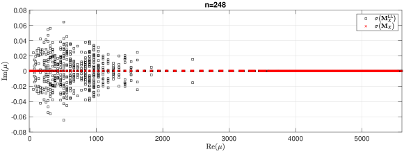
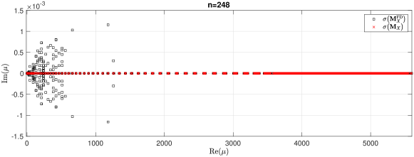
see [12, Proposition 4.4], and that the spectrum of is strictly positive. One of the primary motivations of this paper is to show that similar results hold for CPD kernels and more general operators involving polynomials of . For example, for the simpler case of , we prove that the spectrum of is real and non-negative, as illustrated for a particular in Figure 1 ( markers).
\stackinsetl40ptb18pt
(a) Local Lagrange
\stackinsetl40ptb18pt
(b) RBF-FD
Figure 1: Comparison of the spectra of the DMs for the (negative) Laplace-Beltrami operator on based on the global kernel collocation method () and two local methods: (a) local Lagrange () and (b) RBF-FD (). All results are for the CPD restricted surface spline kernel of order and a minimum energy point set on (described in section 2) with points. Both local DMs were computed using stencils with points. Insets show the spectra near the origin of the complex plane.
A more computationally efficient approach considers instead constructing a DM by approximating using kernel-collocation over local subsets (or stencils) of . One of these techniques uses a “local Lagrange functions”, , generated by a PD or CPD kernel , but only using a small stencil
consisting of points near to , so that for . In this case the DM, which we denote by , is sparse and is given by
(2)
For certain point sets and kernels , is very close to even for relatively small stencils.
This is a consequence of results in [17], which considers local Lagrange bases for certain CPD kernels on spheres (e.g., restricted surface splines), but has been generalized to other kernels on other manifolds [26].
Note that the local Lagrange approach is described in more detail in section 5.2.
Another local technique is the radial basis function finite difference (RBF-FD) method, which has been used widely in many applications on surfaces and general Euclidean domains (e.g. [14, 38, 34, 10, 40, 38]). This method also constructs a sparse DM, which we denote by , but it uses a different stencil-based kernel-collocation approach (as detailed in Section 5.3).
While these local methods are much more computationally efficient than the global method, it is more difficult to prove results about the spectral stability of their DMs because they do not have an underlying structure to exploit. Figure 1 shows that the spectra of DMs of both local methods are indeed more complicated than the global method.
The approach we follow to study the spectral stability of the local DMs is to view them as perturbations of the the global DM, ,
and to bound their spectra in terms of the spectrum of .
Indeed, both local methods recover in the limit that their stencils include every point in .
This motivates two problems:
•
to determine the spectrum for the global DM when is CPD
•
to develop a perturbation theory for the spectrum of kernel-based DMs
Both of these problems are relevant beyond the specific motivation mentioned here. There are many reasons the DM might be perturbed (e.g. by small adjustments to the point set, or
evaluation of the kernel, or by approximation of the differential operator, either
from approximation or by addition of higher order “viscosity” terms),
and it is common practice
to supplement the kernel with an auxiliary polynomial space and provide corresponding
constraints [14, Section 5.1] – in short, to treat a PD kernel as CPD.
Our spectral stability analysis is limited to the local Lagrange DMs , where, for certain kernels and point sets , recent results allow us to bound . Analogous results are not yet available for RBF-FD DMs, but we give numerical evidence that a similar stability analysis may hold.
1.2 Objectives and Outline
The main goals of this article are to produce a perturbation result for global kernel-based DMs on spheres for operators involving polynomials of , and
to employ this result to control the spectrum
of nearby local Lagrange DMs. For strictly PD kernels,
the first goal is achieved by using a fairly straightforward application of the Bauer-Fike theorem. However, the situation is considerably more challenging for CPD kernels, which produce
DMs that are not obviously diagonalizable
(and may have generalized eigenvectors).
However, this is the apposite case for working
with local Lagrange bases on spheres.
A final objective is to show that the
local Lagrange DMs constructed from the restricted surface spline kernels on can have positive spectra.
The outline for the remaining sections of the paper are as follows.
In section 2, we establish notation and give necessary background for spheres, including the spherical Laplace-Beltrami operator, the operators for which our theory applies, PD and CPD kernels on spheres, and point sets.
Section 3 treats the perturbation of the global DMs
generated by PD kernels. The perturbation result follows by estimating the conditioning of the eigenbasis for the DM and applying the Bauer-Fike theorem. This approach can be generalized to other settings (i.e., other
choices of kernel/manifold/differential operator) and we discuss how this might done at the end of section 3.
Section 4 introduces global DMs generated
by CPD kernels.
In section 4.1, we present
Lemma 4.1,
which shows that the
DM for a CPD kernel
is similar to a block-upper-triangular matrix
with diagonal principal blocks.
This factorization is
sufficient to provide
Proposition 4.3, which is
a version of the Bauer-Fike theorem for DMs from CPD kernels.
We then discuss
necessary and sufficient conditions for the DM to be
diagonalizable in section 4.3.
Section 4.4 provides estimates
of the () matrix norms of various blocks appearing in
the decomposition of Lemma 4.1 and
which appear as terms in Proposition 4.3.
Section 4.5 gives experimental evidence
which suggests it is possible to improve the estimates
of some of the matrix norms estimated in section
4.4, and therefore that the
perturbation result Proposition 4.3 can be tightened.
Section 5 provides some applications of the theory from Sections 3 and 4 as well as some numerical results. Energy stability of certain semi-discrete problems is given
in section 5.1. Section 5.2 applies the results of section
4 to the local Lagrange DMs constructed from restricted surface spline kernels on .
In this setting, we show that it is possible to consider a relatively sparse as a perturbation of the global DM that has a closely matching spectrum. In particular, if the spectrum has strictly positive real part, then the spectrum of will also have strictly positive real part for sufficiently large stencils or sufficiently dense point sets . We illustrate these theoretical results on with some numerical examples. Finally, we provide some numerical evidence that similar theoretical estimates may also hold for the RBF-FD DMs .
2 Preliminaries
We denote the d-dimensional sphere as and let denote the Euclidean distance function for .
The sphere has the usual spherical coordinate
parameterization
by where for
and . Here
The Laplace-Beltrami operator on is a self-adjoint, negative semi-definite operator
defined recursively as
where is the Laplace-Beltrami operator on the sphere parameterized
by .
For each ,
is an eigenvalue of the Laplace-Beltrami operator.
The corresponding eigenspace
has an orthonormal
basis of
eigenfunctions,
spherical harmonics
of degree .
Thus
We denote the space of spherical harmonics of degree
as
(3)
and let .
The collection forms an
orthonormal basis for .
Operator
Throughout this article we use to denote
an operator (not differential, per se)
of the form
,
where
is a function which grows at most algebraically.
We define
and note that is diagonalized by
spherical harmonics:
.
If is a polynomial of degree ,
then is a differential
operator of order .
The most elementary choices
are the second order operators generated by
and generated by ,
but there are many
higher order operators which arise in practice:
for the biharmonic, or for the linear part
of the Cahn-Hilliard equation as described in [22],
or higher order powers of the Laplace-Beltrami
as considered for hyperviscosity terms added to differential operators
in order to stabilize kernel-based methods for certain time-dependent PDEs [37].
Point sets
For and finite subset ,
we define the fill distance of in
as
and the separation radius as
In general, the cardinality of can be estimated above and below by
.
A family of point sets is called quasi-uniform
if there is a constant
so that for every in the family, the ratio is bounded by . In this setting,
one has , and thus . Although most of our results hold for general point sets without an a priori bound on the mesh ratio,
some portions (in particular sections 4.4 and 5.1) make use of quasi-uniformity.
For numerical experiments, we employ some benchmark families of
equi-distributed subsets of for our numerical experiments
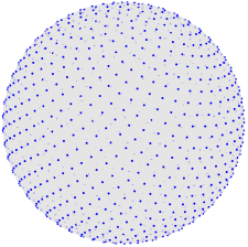
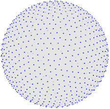
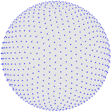
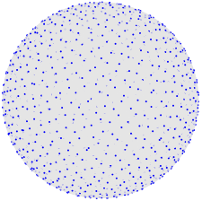
in sections 4.5 and 5.2; namely, Fibonacci, minimum energy, maximum determinant, and Hammersley point sets
(illustrated in Figure 2).
The first three of these sets are quasi-uniform, with separation radii that decay
with the cardinality
like , while the Hammersley points are highly unstructured; see [27] for more information on all of these point sets.
(a) Fibonacci
(b) Min energy
(c) Max determinant
(d) Hammersley
Figure 2: Examples from the point set families on used in the numerical experiments. (a) has points, while for (b)–(d) have points.
Conditionally positive definite kernels
We consider kernels which are
conditionally positive definite (CPD) of order
(i.e., CPD with respect to the spherical harmonic space ).
This means that for any point set , the collocation matrix
(4)
is
strictly positive definite on the space of vectors
A kernel is positive definite (PD)
if for every ,
the collocation matrix (4) is
strictly PD on .
Since such a kernel is CPD with respect to the trivial space
, for ease of exposition we use CPD of order to mean
PD.
For a given point set , define
(5)
The kernels we consider in this paper are zonal, which means
that they have a Mercer-like expansion
(6)
which is absolutely and uniformly convergent.
By the addition theorem for spherical harmonics [32, Theorem 2],
,
where is an algebraic polynomial of degree
with and for all
by [32, Lemma 9].111The functions are orthogonal with respect to the weight , and are thus
proportional to a Gegenbauer polynomials as defined in [1, Chapter 22].
It follows that a series of the form (6) converges uniformly and absolutely on if and only if
the coefficients satisfy
Here we have used the fact that
for and for a -dependent constant .
Note that, by [31, Theorem 4.6],
an expansion of the form (6)
yields a
kernel which is CPD of order if and only
the expansion coefficients satisfy for all , and
for infinitely many odd and infinitely
many even values of (the
PD
case (i.e., ) was given in
[8, Theorem 3]).
However, most
CPD
kernels of interest have the property that
for all .
We direct the reader to [4] for a number of prominent examples of
kernels (both PD and CPD)
with precisely calculated coefficients .
Compatibility assumption between and
For a kernel , and a differential operator ,
we adopt the convention that
means that the operator is applied to the first argument, i.e.,
.
The following assumption guarantees
that is CPD and
that is a zonal kernel.
It is in force throughout this paper.
Assumption 2.1.
Let denote
a kernel
with a Mercer-like expansion (6),
which is CPD of order (where means is PD).
Let be a linear operator
obtained by
so that the eigenvalues
grow at most algebraically, and that
.
Note that some of these assumptions have already been mentioned earlier in this section – the critical
hypothesis is the compatibility condition between and ,
namely .
This condition can be further simplified if is a differential operator of order
(in other words, if is polynomial of degree or less).
The requirement that
converges can be expressed in this case as
.
Miscellaneous notation
Throughout the paper, we let (with or without subscripts) denote a generic positive constant.
To denote matrices, we use bold upper case letters. We also use to denote the induced matrix norm.
3 Spectral stability for PD kernels
If Assumption 2.1 holds with ,
we define the global DM
for the
finite point set
as the unique matrix in which satisfies the identity
for all .
It has the form
It follows that is a
symmetric matrix generated by sampling
.
We can thus conclude that
the spectrum of is the same as that of the symmetric matrix
.
In particular, if has non-negative spectrum (each ),
then is positive semi-definite, so .
Furthermore, if
for infinitely many odd and infinitely many even ,
then is strictly positive definite, and .
3.1 Conditioning of the eigenbasis of
While the above setup shows that is diagonalizable
and we have control on ,
the eigenvectors of may be far from orthogonal.
To understand the conditioning of the eigenbasis of ,
we consider the matrix
which, by the above factorization, satisfies
,
and is therefore symmetric.
Proposition 3.1.
Suppose Assumption 2.1 holds with .
If
has cardinality
and if
then for every eigenvalue
of ,
there is an eigenvalue of with
where
is the condition number of .
Proof.
By the above comment,
with an orthogonal matrix.
Hence, we have a diagonalization of the form
with .
As is orthogonal,
satisfies
The result then follows by an application of
the Bauer-Fike theorem [3].
∎
In case has coefficients which have prescribed algebraic decay ,
it is possible to control the smallest eigenvalue of the collocation matrix by a power of
the separation radius .
This situation corresponds to a number of kernels with Sobolev native spaces, including
compactly supported kernels and restricted Matérn kernels, as described in [12, Appendix].
Corollary 3.2.
Suppose the hypotheses of Proposition 3.1 hold, and
the expansion coefficients of satisfy
.
Then
for every eigenvalue
of ,
there is an eigenvalue of with
Proof.
By [12, Lemma 4.2],
the decay of the coefficients allows us
to bound
by , while
since is bounded and .
Thus
and the corollary follows.
∎
Note that if and is a polynomial of degree or less,
so is a differential operator of
order , then
the summability condition from
Assumption 2.1
is equivalent to
.
3.2 Generalizations to other settings
The above setup can be generalized considerably to other manifolds
and operators .
We begin by assuming that the underlying set
is a metric space with distance function
.
If
is one of a countable collection of continuous functions whose span is
dense in then any series
(8)
which converges absolutely and uniformly
is PD
if
for every .
In particular, the collocation matrix
is positive definite for any finite set .
If is a linear operator diagonalized by the ’s,
i.e.,
and for which the series
converges absolutely and uniformly, then the DM
has the form
where is symmetric,
and
the perturbation
result of Proposition
3.1 holds in this setting.
Example 1: (intrinsic) compact Riemannian Manifolds
A common setup involves a compact, -dimensional
Riemannian manifold endowed
with Laplace-Beltrami operator, given in intrinsic coordinates as
In this case, there exists
a countable orthonormal basis
of eigenvectors of
with corresponding eigenvalues .
We may assume each
to be real-valued.
In this setting, we may again let for a function
defined on .
The requirement of absolute and uniform convergence
of the series
may be simplified by using Weyl laws to control the growth of .
Estimates in the uniform norm of eigenfunctions can be obtained in specific
cases, see e.g. [39, Theorem 2.1] or [11].
There are two immediate challenges to this approach.
The first comes purely from adapting Corollary 3.2.
In order to estimate the condition number of the eigenbasis
in terms of
the separation radius .
As in the case , this can be controlled by estimating the minimal eigenvalue
of the collocation matrix .
To control this eigenvalue one may attempt to adapt [12, Lemma 4.2],
although the much more general spectral theoretic arguments of [23], specifically
[23, Proposition 8] may be more easily adapted to this setting.
The second challenge stems form using the kernel and the DM .
Although nicely defined by a series, the kernel
may not have a convenient closed-form representation.
This challenge can be addressed if the eigenfunctions appearing in (8) are known.
If this is the case, it may be suitable to truncate the Mercer-like series at a sufficiently large threshold .
Of course, truncating the kernel imposes some error which would need to be managed (for instance
by way of perturbation results like Corollary 3.2).
Example 2: embedded compact Riemannian Manifolds
If is a compact Riemannian manifold
embedded in Euclidean space, we may follow [18]
by considering
a radial basis function (RBF)
,
namely a function which is symmetric under rotations
(i.e., for some function )
and has Fourier transform which satisfies
for some .
In that case, is a PD kernel on .
By Mercer’s theorem,
it has an absolutely and uniformly convergent
expansion of the form (8), where
the functions are eigenfunctions of the integral
operator .
The challenge in this case is that
closed form expressions for the eigenfunctions
’s and coefficients are not known in general (see
[36] for an approach to
approximate these).
As a result, it is difficult to identify
the operators
diagonalized by which are necessary
to apply Proposition 3.1.
In contrast to the case of Example 1,
[43, Theorem 12.3] guarantees that
the collocation matrix has minimal eigenvalue
,
so
.
On
the other hand
is guaranteed
by the continuity of
and the compactness of ,
so an analogue of Corollary 3.2 holds in this case
with estimate
4 Spectral stability for CPD kernels
We now present our main results for
global DMs constructed using CPD kernels.
In section 4.1
we show that is similar to
the sum of a diagonal matrix
and nilpotent matrix
with a single nonzero block.
This is Lemma 4.1.
In section 4.2 we give a preliminary version
of the Bauer-Fike theorem which treats the block triangular
factorization.
Section 4.3
considers the full diagonalization of
under mild assumptions on the operator .
We analyze the norms of various factors
appearing in the factorization in Section 4.4.
4.1 DM block decomposition
For a CPD kernel of order and operator
which satisfy Assumption 2.1,
and for a point set ,
define the DM so that
holds for all .
Then can be expressed as
(9)
where
and
is an Vandermonde
matrix associated with a basis for (see (3)).
Here we take
,
for a suitable enumeration , so that is the diagonal matrix such that
.
The matrices
and occur as solutions
to the augmented kernel collocation problem
(10)
where
is the kernel collocation matrix.
The kernel collocation matrix is a saddle-point matrix and we
will exploit this structure and known facts for those matrices
as they can be found for instance in [6] later on.
Let be the standard left inverse
of and
be the orthogonal projector onto the space where
Let be a matrix whose columns
form an orthonormal basis for .
Then .
The first equation shows that is positive semi-definite
and that
(13)
From (12), we can begin to decompose , obtaining first
(14)
Adding and subtracting
,
we write the second term in (14) as
The first term in this expression is ,
which equals by (13).
This gives the identity:
(15)
The first term in (15)
corresponds to a diagonalizable block.
Indeed, restricting to the invariant subspace
yields
for
.
The second term in (15) can also be viewed as a block of ,
this time restricted to (recall that annihilates ).
Indeed,
can be diagonalized, as we did in section 3.1.
This can be made more explicit with a change of basis using .
Change of basis
For a matrix , let
(16)
Recall that the columns of form an
orthonormal basis for . Thus
and
its inverse
are both positive definite.
By the same reasoning,
is symmetric, and if for , then
is positive semi-definite.
If, in addition,
for infinitely many even values
of and infinitely many odd values of ,
then
[31, Theorem 4.6] guarantees that
is strictly positive definite
(this occurs, for instance, if and is a polynomial).
This yields the following result.
Lemma 4.1.
If Assumption 2.1
holds with
and is finite,
then
the DM
has factorization
where
and
are
diagonal, and each entry
is
determined by the spectrum of on ; i.e.,
with
where .
If for all , then each diagonal entry of is non-negative, and if, furthermore,
for infinitely many even and infinitely many odd values of ,
then each diagonal entry of
is strictly positive.
Finally, we note that if for all , then
is positive semi-definite, and
so is
.
This implies that
,
is positive semi-definite.
Since is diagonal,
each .
The last statement follows from the observation that is positive definite in this case.
∎
Remark 4.2.
As a consequence of Lemma 4.1 we obtain that
for an operator with also for a CPD kernel of order .
More quantitative results will be shown in Lemma 4.4.
4.2 A generalization of the Bauer-Fike Theorem
By adapting the argument from [9],
we obtain the following estimate on perturbation of eigenvalues of .
so the block upper triangular matrix is diagonalizable.
There are practical solution methods for problems of the form (27)
under significantly more general conditions than we use
(just the assumption that the spectra of
and
are separated, see [7, 2]
and [28] for an overview).
In our case, where and are diagonal, the
solution is very simple.
We may rewrite (27) with the help of the matrix
.
In that case, (27) has the form
, where is entry-wise multiplication.
This leads to three cases:
1.
The spectra of and are disjoint,
in which case has no zero entries, and
has a unique solution obtained by entry-wise division.
2.
There is some overlap between spectra of and ,
but each zero entry of corresponds
to a zero entries of .
In this case, there are many solutions to (27).
3.
and ,
have overlapping spectra and
for some for which .
In this case,
has a generalized eigenvector.
If either case 1. or 2. holds, then (27) has a solution
Under basic hypotheses on the operator , we can estimate the separation between and , and therefore
we can estimate the norm of .
and where .
The condition number for the eigenbasis is controlled by
.
We can estimate .
The result then follows from the standard Bauer-Fike theorem.
∎
4.4 Matrix norms of elements of the block decomposition
We now restrict the situation to
kernels which are CPD of order
and for which
the coefficients in the expansion (6) satisfy
for all .
Estimating
and
We can estimate
via Hölder’s inequality.
so
.
Since is assumed to be fixed and ,
we can express this estimate as
A simple consequence of
[33, Theorem 4.2] guarantees that
the Gram matrix
has spectrum contained in the interval
for constants and independent of
(see [12, Lemma 4.2]
for this argument in the case ).
It follows that
,
where is the mesh ratio of ,
and is a constant that only depends on and .
Thus,
(30)
Estimating
and
By [17, Proposition 5.2], the minimal eigenvalue
of
is bounded below by
for some constant .
Additionally, since is the positive square root of and
The latter two use the matrix norms
and , which can be
estimated by introducing supremum norms
and ,
to obtain
and .
Recalling that ,
we obtain the bound
(31)
It is conceivable that a much better estimate is possible, since
the factor
,
which involves a commutator-like factor
(namely ),
has been roughly estimated with a triangle inequality.
We investigate this numerically in the next section.
Estimating the condition number of
We now consider the condition number
appearing in Lemma 4.3.
The blocks and of
have orthogonal ranges and nullspaces.
Indeed, we have
and
Thus,
and
.
It follows that
If ,
we have
Together, this implies
Corollary 4.6.
Under hypotheses of Proposition 4.3, if
we assume the kernel’s expansion coefficients
satisfy
for all
and ,
then for a matrix
sufficiently close to ,
and
there is a for which
Proof.
Plugging the estimate
into Proposition 4.3 gives
the first inequality.
Using the bound (31)
for
gives
the second.
∎
4.5 Numerical estimates on
In this section, we give numerical evidence that much better estimates for than (31) may be possible.
We consider DMs for on using the four families of point sets discussed in section 2 and illustrated in Figure 2.
(a) Fibonacci
(c) Maximum determinant
(b) Minimum Energy
(d) Hammersley
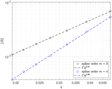
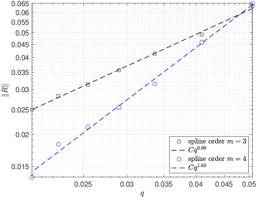
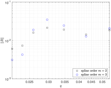
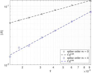
Figure 3: Numerical results on vs. the separation radius for different point set families on using . Each plot shows the results for the restricted surface (32) spline kernels of order and using augmented spherical harmonic spaces . The dashed lines in (a), (c), & (d) show the lines of best fit (on a log-scale) to the data, which indicate an algebraic decay rate of with decreasing . The results in (b) do not show a discernible pattern of in terms of , so the estimated rates are omitted.
We first consider DMs formed from the restricted surface spline kernels:
(32)
These kernels are CPD of order , where , and have
a Mercer-like expansion (6) with
coefficients that decay like
for .
Indeed, for , the kernel has expansion (6)
with coefficients satisfying
by [25, Lemma 3.4]. We consider the and kernels with augmented spherical harmonic spaces (the minimum degree space required for well-posedness). Figure 3 displays the results of computed for points of increasing cardinality (and hence decreasing ) from each family of point sets. Included in the plots from (a), (c), & (d) of this figure are the estimated algebraic rates of decay of in terms of decreasing ; these estimates were omitted from (b) since no discernible pattern was evident. We note that the estimated rates in the three figures all involve positive powers of rather than negative powers as in the bound (31). Furthermore, even the results in (b) do not follow (31).
(a) surface spline
(b) inverse multiquadric
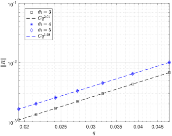
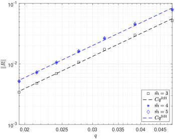
Figure 4: Numerical results on vs. the separation radius for the Fibonacci points on using . (a) Results from three experiments with the order of the restricted surface spline kernel (32) fixed at and the degree of augmented spherical harmonic spaces changing. (b) Same as (a), but for the restricted inverse multiquadric kernel. Dashed lines estimate the algebraic decay rate of with decreasing .
In the next experiment we test how depends on the degree of the augmented spherical harmonic basis , , when the kernel is fixed. This is especially common for applications of kernel-based methods on (and more general domains) where the order of the spline kernel is kept low and the degree of the polynomial basis is allowed to grow [37, 5]. Figure 4 (a) shows the results for the Fibonacci nodes. We see from this plot that increasing the degree does not change the algebraic rate of decay of with decreasing , but only (possibly) the constant. We note that similar results were observed for the maximum determinant and Hammersley points and are thus omitted.
Finally, we consider the behavior of for the restricted inverse multiquadric kernel , where is the free shape parameter. This kernel is PD with coefficients in (6) that decay exponentially fast with [4]. Hence, the estimates for bounding in (31) do not apply. Figure 4 (b) displays the results associated with this kernel using the Fibonacci nodes. Similar to part (a) we include results for when including different augmented spherical harmonic bases with this kernel. As with the restricted surface spline results, seems to have an algebraic decay rate (of approximately 3) with decreasing and this rate does not seem to depend on . We note that similar results were observed (with different algebraic rates) for the other point set families and hence are omitted.
These experiments suggest that the estimate in (31) is indeed overly pessimistic and better bounds for may be possible, even ones that extend to kernels with exponentially decaying Mercer expansions. Unfortunately, the geometry of the points seems to affect the algebraic decay of with decreasing , so any tighter estimates may need to take the geometry into account.
5 Applications
In this section consider two applications of the theory of sections 3 and 4.
5.1 Continuous time-stability for the global DMs
Consider the semi-discrete approximation of the equation at a set of points , where and (e.g., for corresponding to the diffusion equation). We denote the approximation as
(33)
where and is the global DM associated with a PD or CPD kernel .
A straightforward application of the results from sections 3 and 4 can be used to show the solution of the semi-discrete system is energy stable, and thus the norm of does not grow in time. The proofs differ depending on the kernel used to construct .
PD Kernel
Using the norm ,
we note that
which implies, using (7) that
,
so the semi-discrete problem (33) is energy stable.
CPD Kernel
In this case, we employ the
semi-norm
where is the positive semi-definite matrix given in (11).
Then
which implies, since , that
Here we have used (13) and the change of basis (16).
Since has negative spectrum,
we have
as long as
. However, if
, then ,
in which case is exact and we can use the standard norm to show . Thus, the semi-discrete problem (33) is energy stable also for the CPD case.
5.2 Spectral stability of the local Lagrange DMs from restricted surface splines
We apply the results of section 4 to
the restricted surface spline kernels
on defined in
(32).
Recall that is CPD of order as long as .
When , these kernels have the property, introduced in [17],
that for quasi-uniform point sets ,
the kernel spaces
possess a
localized basis:
a basis , which enjoys the following two properties
(among others)
•
each function employs a small stencil:
where consists of points near to ,
•
each
is close to in a variety of norms (roughly, for
the norm of any Banach space in which the native space is embedded
– this will be made more precise below).
The sphere, along with Euclidean space, provides the most readily
available kernels having localized bases, although they exist in other
settings as well. For any general compact, closed Riemannian manifold,
there exist PD kernels with this property, as shown in [26],
although they generally do not have convenient closed form expressions,
or even expansions of the form (6) in a familiar orthonormal set.
For compact, rank 1 symmetric spaces
(which include spheres of all dimensions,
as well as a number of other sphere-like manifolds),
there exist kernels with Mercer-like expansions
in the Laplacian eigenbasis, as shown in [24],
for which the ideas of [17] can be applied to
construct localized bases – in particular, this is possible for
restricted surface splines and similar kernels
on higher dimensional spheres.
Perturbation of the DM via localized bases
Let have mesh ratio .
For , and for ,
we define the stencil ,
and note that has cardinality
.
We define
the local Lagrange function
via the condition
Note that ,
since .
By [12, Lemma 5.2], there exist positive constants and so that
for any stencil parameter
and
for sufficiently dense ,
The local Lagrange DM, , is constructed by applying to each :
Since has mesh-ratio
the stencil has cardinality
.
Thus
there are nonzero
entries in each row (or column) of .
Following the arguments in [12],
specifically estimates [12, (6.3)] and [12, (5.9)],
we have that
(34)
We note that the approximation
order given by (34)
has an linear dependence on the stencil parameter ,
namely for some , with .
We can measure the distance between spectra of and
by using either Proposition
4.3 in the most general setting,
or Theorem 4.5
in cases where separates from its orthogonal complement.
General (non-diagonalized) case
We apply Proposition 4.3,
with , and observe
that for every eigenvalue
there is
for which
.
At this point, we use the estimates on ,
and
collected in Corollary 4.6 to note that
This suggests that (and therefore )
should be chosen
larger than in order to ensure fidelity
to the original
(positive) spectrum of .
Remark 5.1.
If the pessimistic bound is replaced
by ,
as suggested by the experimental results
of section 4.5,
then Corollary 4.6 gives the improved estimate
Diagonalizable case
If satisfies
,
then we may apply
Theorem 4.5
to obtain
In particular, this holds if .
(We recall that in this section
we require .)
Remark 5.2.
Here, as in Remark 5.1,
if
is replaced
by ,
as suggested by the experimental results
of section 4.5,
then Theorem 4.5 gives the improved estimate
5.2.1 Numerical results on spectra of the local Lagrange DMs
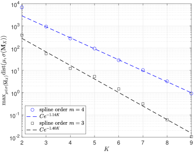
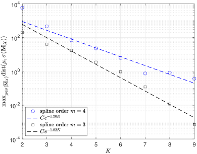
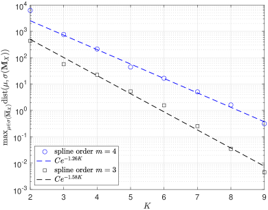
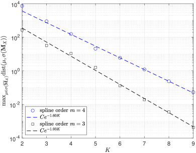
(a) Fibonacci
(c) Maximum determinant
(b) Minimum Energy
(d) Hammersley
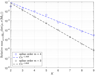
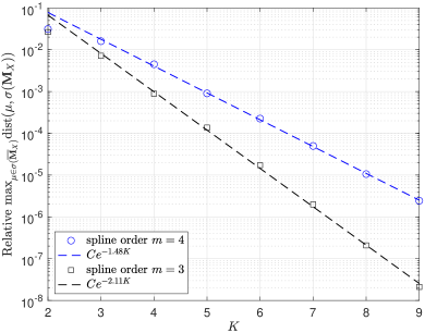
Figure 5: Numerical results comparing the maximum of the minimum distances between the spectra of the global DM () and local Lagrange DM () as a function of the parameter controlling the stencil size of the local Lagrange basis. Results are for computed from the restricted surface splines (32) of order and with augmented spherical harmonic spaces . Dashed lines are the lines of best fit (on a log-linear scale) to the data for , which indicate an exponential decay rate with increasing .
The results from the previous section
show that
(35)
can be controlled by an expression of the form
where , although the precise dependence of and
on and are not
easily determined analytically.
In this section, we numerically examine the exponential decay of these bounds in terms of for .
Rather than choosing the support points in each stencil from a ball search with a radius that depends on , we use a nearest neighbor search so that the cardinality of each stencil is fixed at
(36)
For a quasi-uniform point set , this gives similar results to a ball search. Additionally, this nearest neighbor approach with a fixed stencil size is more common in RBF-FD methods [14].
We again use the four families of point sets described in section 2 (and displayed in
Figure 2): Fibonacci, minimum energy, maximum determinant, and Hammersley. As discussed in that section, the first three of these are quasi-uniform so the theory from the previous section applies. We also include results on the Hammersley points to see if this theory can potentially be generalized to more general point sets. For the numerical experiments we set for all but the Fibonacci nodes, where since they are only defined for odd numbers.
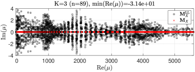
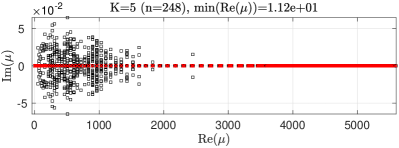
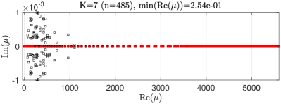
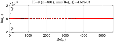
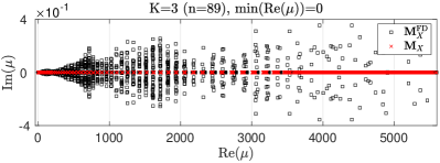
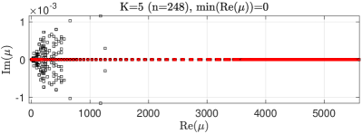
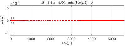
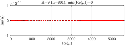
Figure 6: Comparison of the spectra of the global () and local Lagrange () DMs based on different stencil sizes. Results are for the with minimum energy points and the kernel is the restricted surface spline kernel of order . The minimum real part of spectrum of is listed in the title of each plot . Note the different scales for the vertical (imaginary) axes on each plot.
Figure 5 displays the results from the experiments for the restricted surface spline kernels of orders and . We see from the figure that distance between the spectra (35) decreases exponentially fast with for all four families of point sets, but that the rate depends on the geometry of the point set. We also see that the decay rate depends on the order of the kernels as the estimates from the previous section predict.
To better compare the spectra of and , we plot the entire spectrum of each matrix for the minimum energy points and four different values in Figure 6. We see from the plots in this figure that as increases the spread of the eigenvalues of in the complex plane decreases. Additionally, for this point set, the real part of the spectrum of is non-negative for all but the case (see in the titles of the plots of the spectra).
5.3 Numerical results on spectra of the RBF-FD DMs
(a) Fibonacci
(c) Maximum determinant
(b) Minimum Energy
(d) Hammersley
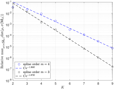
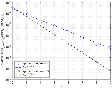
Figure 7: Same as Figure 5, but for the RBF-FD DM ().
The RBF-FD method is similar to the local Lagrange method in that it produces a sparse DM, , for approximating at a set of points using kernel interpolation over local stencils of points. However, unlike the local Lagrange case, estimates are not yet available for bounding so that the results of Proposition
4.3 or Theorem 4.5 can be applied to the spectral stability of . In this section we numerically compare the stability of in terms of using (36) to give evidence that similar bounds to the ones from Section 5.2 for hold.
First, we briefly review the RBF-FD method for the case of surface splines on ; see [14] for more general settings and details. Let again denote a local stencil of points for each , and be some generic function. To approximate the operator at , the RBF-FD method uses
where are stencil Lagrange functions associated with and is the index set for the stencil in the global node set . The stencil Lagrange functions are in the space defined in (5) and satisfy for . The entries of RBF-FD DM are then given as follows:
The difference between the local Lagrange and RBF-FD methods may be subtle, but it is important. The latter is based on a separate interpolant over the stencil defined by the target point , while the former is based on interpolants defined over all stencils that have a non-empty intersection with the target point . The RBF-FD method is then necessarily exact on the space , but the local Lagrange method is not. We finally note that both methods produce in the limit that each stencil includes every point in , i.e., .
For the numerical results, we follow exactly the same set-up as the previous section and compare the spectra of to using the measure (35) for different and surface spline orders . We note that since is exact on its spectrum will included , where are the first eigenvalues of .
Figure 8: Same as Figure 6, but for the RBF-FD DM ().
Figure 7 displays the results from the experiments. Similar to the local Lagrange case, we see from the figure that the distance between the spectra (35) for also decreases exponentially fast with for all four families of point sets. This indicates that similar bounds to those from Section 5.2 for may also hold for .
The spectra of and are directly compared in Figure 8 for the minimum energy points. We see from this figure that for the same the spectrum of does not extend as far in the complex plane as the spectrum of given in Figure 6. Additionally, the rate at which the spectrum approaches the positive real axis as increases is higher for the RBF-FD method. Finally, the figure shows that for each the eigenvalue of with the smallest real part is 0, which is the expected value for .
6 Concluding remarks
The results of this paper have addressed important issues regarding the spectrum of DMs that arise in global and local kernel collocation methods and their stability under perturbations. However, there remain significant open questions in both the global and the local cases. We briefly note three interesting open problems:
•
There is more to temporal stability of method of lines (or semi-discrete) approximations like (33) considered in section 5.1 than the spectrum of the DM or the energy stability of the solutions of (33). Showing stability for the fully discrete problem (i.e., after discretizing (33) in time) requires addressing questions about the pseudospectra (resolvent stability) [42] or strong stability [30] of the DMs. In the latter case, [30, Section 3.1] considers the coercivity condition
of a matrix in some inner product (this is[30, (3.2)]). Coercivity guarantees stability of certain Runge-Kutta method applied to (33) provided a CFL-type condition holds.
•
If and , then
a perturbed DM may fail to inherit the Hurwitz stability of .
In short, the results presented here do not guarantee that perturbation preserves
weak Hurwitz stability (semi-stability).
•
The challenge of obtaining useful perturbation errors for that are similar to (34) amounts to controlling
the difference .
Superficially, this may seem similar to
, but the challenge
stems from the fact that the center associated with
may be
situated near to the boundary of the domain of
, which is
where the decay conditions of the Lagrange
functions are not yet well understood.
References
[1]
Milton Abramowitz and Irene A Stegun.
Handbook of mathematical functions with formulas, graphs, and
mathematical tables, volume 55.
National bureau of standards, 1964.
[2]
Richard H. Bartels and George W Stewart.
Solution of the matrix equation AX+ XB= C [f4].
Communications of the ACM, 15(9):820–826, 1972.
[3]
Friedrich L Bauer and Charles T Fike.
Norms and exclusion theorems.
Numerische Mathematik, 2:137–141, 1960.
[4]
Brad JC Baxter and Simon Hubbert.
Radial basis functions for the sphere.
In Recent Progress in Multivariate Approximation: 4th
International Conference, Witten-Bommerholz (Germany), September 2000, pages
33–47. Springer, 2001.
[5]
Victor Bayona, Natasha Flyer, Bengt Fornberg, and Gregory A Barnett.
On the role of polynomials in RBF-FD approximations: II.
Numerical solution of elliptic PDEs.
J. Comput. Phys., 332:257–273, 2017.
[6]
Michele Benzi, Gene H Golub, and Jörg Liesen.
Numerical solution of saddle point problems.
Acta numerica, 14:1–137, 2005.
[7]
William Gee Bickley and J McNamee.
Matrix and other direct methods for the solution of systems of linear
difference equations.
Philosophical Transactions of the Royal Society of London.
Series A, Mathematical and Physical Sciences, 252(1005):69–131, 1960.
[8]
Debao Chen, Valdir Menegatto, and Xingping Sun.
A necessary and sufficient condition for strictly positive definite
functions on spheres.
Proceedings of the American Mathematical Society,
131(9):2733–2740, 2003.
[9]
King-wah Eric Chu.
Generalization of the Bauer-Fike theorem.
Numerische Mathematik, 49:685–691, 1986.
[10]
Oleg Davydov.
Error bounds for a least squares meshless finite difference method on
closed manifolds.
Advances in Computational Mathematics, 49(4):48, 2023.
[11]
Harold Donnelly.
Bounds for eigenfunctions of the Laplacian on compact Riemannian
manifolds.
Journal of Functional Analysis, 187(1):247–261, 2001.
[12]
Wolfgang Erb, Thomas Hangelbroek, Francis J. Narcowich, Christian Rieger, and
Joseph D. Ward.
Highly localized RBF Lagrange functions for finite difference
methods on spheres, 2023.
[13]
Natasha Flyer and Grady B Wright.
A radial basis function method for the shallow water equations on a
sphere.
In Proceedings of the Royal Society of London A: Mathematical,
Physical and Engineering Sciences, pages rspa–2009. The Royal Society,
2009.
[14]
B. Fornberg and N. Flyer.
Solving PDEs with radial basis functions.
Acta Numer., 24:215–258, 2015.
[15]
B. Fornberg and E. Lehto.
Stabilization of RBF-generated finite difference methods for
convective PDEs.
Journal of Computational Physics, 230:2270–2285, 2011.
[16]
Bengt Fornberg and Natasha Flyer.
A Primer on Radial Basis Functions with Applications to
the Geosciences.
Society for Industrial and Applied Mathematics, Philadelphia, PA,
USA, 2015.
[17]
E. Fuselier, T. Hangelbroek, F. J. Narcowich, J. D. Ward, and G. B. Wright.
Localized bases for kernel spaces on the unit sphere.
SIAM J. Numer. Anal., 51(5):2538–2562, 2013.
[18]
Edward Fuselier and Grady B Wright.
Scattered data interpolation on embedded submanifolds with restricted
positive definite kernels: Sobolev error estimates.
SIAM Journal on Numerical Analysis, 50(3):1753–1776, 2012.
[19]
Edward J Fuselier and Grady B Wright.
A high-order kernel method for diffusion and reaction-diffusion
equations on surfaces.
Journal of Scientific Computing, 56(3):535–565, 2013.
[20]
Q. T. Lê Gia.
Approximation of parabolic PDEs on spheres using spherical basis
functions.
Adv. Comput. Math., 22:377–397, 2005.
[21]
Jan Glaubitz, Jan Nordström, and Philipp Öffner.
Summation-by-parts operators for general function spaces.
SIAM Journal on Numerical Analysis, 61(2):733–754, 2023.
[22]
John B Greer, Andrea L Bertozzi, and Guillermo Sapiro.
Fourth order partial differential equations on general geometries.
Journal of Computational Physics, 216(1):216–246, 2006.
[23]
Michael Griebel, Christian Rieger, and Barbara Zwicknagl.
Regularized kernel-based reconstruction in generalized besov spaces.
Foundations of Computational Mathematics, 18:459–508, 2018.
[24]
T. Hangelbroek, F. J. Narcowich, and J. D. Ward.
Polyharmonic and related kernels on manifolds: interpolation and
approximation.
Found. Comput. Math., 12(5):625–670, 2012.
[25]
Thomas Hangelbroek.
Polyharmonic approximation on the sphere.
Constructive Approximation, 33(1):77–92, 2011.
[26]
Thomas Hangelbroek, Francis J Narcowich, Christian Rieger, and Joseph D Ward.
Direct and inverse results on bounded domains for meshless methods
via localized bases on manifolds.
Contemporary Computational Mathematics-A Celebration of the 80th
Birthday of Ian Sloan, pages 517–543, 2018.
[27]
D. P. Hardin, T. Michaels, and E. B. Saff.
A comparison of popular point configurations on .
Dolomites Res. Notes Approx., 9:16–49, 2016.
[28]
Nick Higham.
What is the Sylvester equation?
https://nhigham.com/2020/09/01/what-is-the-sylvester-equation/.
[29]
E Lehto, V Shankar, and G. B. Wright.
A radial basis function (RBF) compact finite difference (FD)
scheme for reaction-diffusion equations on surfaces.
SIAM J. Sci. Comput., 39:A219–A2151, 2017.
[30]
Doron Levy and Eitan Tadmor.
From semidiscrete to fully discrete: Stability of Runge–Kutta
schemes by the energy method.
SIAM review, 40(1):40–73, 1998.
[31]
Valdir Antônio Menegatto and Ana Paula Peron.
Conditionally positive definite kernels on euclidean domains.
Journal of mathematical analysis and applications,
294(1):345–359, 2004.
[33]
Francis J Narcowich, Pencho Petrushev, and Joseph D Ward.
Localized tight frames on spheres.
SIAM Journal on Mathematical Analysis, 38(2):574–594, 2006.
[34]
Dang Thi Oanh, Oleg Davydov, and Hoang Xuan Phu.
Adaptive rbf-fd method for elliptic problems with point singularities
in 2d.
Applied Mathematics and Computation, 313:474 – 497, 2017.
[35]
Rodrigo B Platte and Tobin A Driscoll.
Eigenvalue stability of radial basis function discretizations for
time-dependent problems.
Computers & Mathematics with Applications, 51(8):1251–1268,
2006.
[36]
Gabriele Santin and Robert Schaback.
Approximation of eigenfunctions in kernel-based spaces.
Advances in Computational Mathematics, 42:973–993, 2016.
[37]
Varun Shankar and Aaron L. Fogelson.
Hyperviscosity-based stabilization for radial basis function-finite
difference (RBF-FD) discretizations of advection-diffusion equations.
J. Comput. Phys., 372:616–639, 2018.
[38]
Varun Shankar, Grady B. Wright, Robert M. Kirby, and Aaron L. Fogelson.
A radial basis function (RBF)-finite difference (FD) method for
diffusion and reaction-diffusion equations on surfaces.
J. Sci. Comput., 63(3):745–768, 2014.
[39]
Christopher D Sogge.
Concerning the norm of spectral clusters for second-order
elliptic operators on compact manifolds.
Journal of Functional Analysis, 77(1):123–138, 1988.
[40]
Igor Tominec, Elisabeth Larsson, and Alfa Heryudono.
A least squares radial basis function finite difference method with
improved stability properties.
SIAM Journal on Scientific Computing, 43(2):A1441–A1471, 2021.
[41]
Igor Tominec, Murtazo Nazarov, and Elisabeth Larsson.
Stability estimates for radial basis function methods applied to
time-dependent hyperbolic pdes.
arXiv preprint arXiv:2110.14548, 2021.
[42]
Lloyd N. Trefethen and Mark Embree.
Spectra and Pseudospectra: The Behavior of Nonnormal Matrices
and Operators.
Princeton University Press, Princeton, 2005.
[43]
Holger Wendland.
Scattered data approximation, volume 17.
Cambridge university press, 2004.
[44]
Holger Wendland and Jens Künemund.
Solving partial differential equations on (evolving) surfaces with
radial basis functions.
Advances in Computational Mathematics, 46:64, 2020.