Augmented bridge matching

Abstract

Flow and bridge matching are a novel class of processes which encompass diffusion models. One of the main aspect of their increased flexibility is that these models can interpolate between arbitrary data distributions, i.e. they generalize beyond generative modeling and can be applied to learning stochastic (and deterministic) processes of arbitrary transfer tasks between two given distributions. In this paper, we highlight that while flow and bridge matching processes preserve the information of the marginal distributions, they do not necessarily preserve the coupling information unless additional, stronger optimality conditions are met. This can be problematic if one aims at preserving the original empirical pairing. We show that a simple modification of the matching process recovers this coupling by augmenting the velocity field (or drift) with the information of the initial sample point. Doing so, we lose the Markovian property of the process but preserve the coupling information between distributions. We illustrate the efficiency of our augmentation in learning mixture of image translation tasks.

1 Introduction

Diffusion models (Song & Ermon, 2019; Ho et al., 2020; Sohl-Dickstein et al., 2015) have recently emerged as state-of-the-art models in generative modeling for diverse modalities: from text-to-images (Saharia et al., 2022b), 3D (Poole et al., 2022), video (Ho et al., 2022) and protein synthesis (Watson et al., 2022). They rely on an iterative procedure, where the target data distribution is first corrupted using a forward noising process converging to a Gaussian distribution. Then, the time-reversal of this process is learned leveraging techniques from score-matching (Hyvärinen & Dayan, 2005; Vincent, 2011).

Diffusion models have recently been adapted to tackle general inverse problems. In that case, several frameworks have been proposed: from classifier and classifier-free guidance (Dhariwal & Nichol, 2021; Ho & Salimans, 2022; Chung et al., 2022b; a), with or without Sequential Monte Carlo correction (Trippe et al., 2022), to the replacement method in the context of inpainting (Lugmayr et al., 2022) or Denoising Diffusion Restoration Models (Kawar et al., 2022). While these models have been successful they can be seen as guided modifications of diffusion models and in particular, at inference time, the output is still initialized with Gaussian noise. In the context of inverse problems where one observes a corrupted sample and tries to recover a clean version, it is desirable to instead start the inference from the corrupted sample. However, this requires changing the target distribution of the forward process which is often intractable and leads to numerical difficulties.

To circumvent this issue, Lipman et al. (2022); Peluchetti (2021) have introduced a generalization of diffusion models called flow matching (we call bridge matching its stochastic counterpart) which interpolates between two distributions. In particular, both endpoints of the process are fixed by the user and the specific application. If the terminal distribution is given by the output of the forward noising process, then we recover diffusion models. However, bridge matching procedures are more flexible and recent works have leveraged them to solve inverse problems (Somnath et al., 2023; Liu et al., 2023; Delbracio & Milanfar, 2023; Tong et al., 2023; Albergo et al., 2023; Chung et al., 2023; Heitz et al., 2023). In that case, we learn the velocity field of an Ordinary Differential Equation (ODE), or the drift of a Stochastic Differential Equation (SDE), between degraded and clean samples. To train such models, we assume that we have access to a coupled dataset. This means that we can draw samples $(x_{0},x_{1})$ from a joint distribution. In particular, the training process assumes the knowledge of a certain coupling between the two data distributions.

In this work, we answer the following question: does the flow/bridge matching procedure preserve the coupling information? We already know from Gyöngy (1986) that it preserves the marginal information. This is because both flow and bridge matching can be seen as specific instances of a Markovian projection (Shi et al., 2023) which enjoys desirable properties. On the other hand, it has been shown that the flow matching procedure provides a coupling which has a lower cost than the original one for every convex cost (Liu, 2022). As a first contribution, we show that the Markovian projection in fact preserves the trajectories if and only if the original coupling is the entropic regularized optimal transport one, i.e. a static Schrödinger bridge. Since in practice, available datasets of paired clean/corrupted samples are not ensured to satisfy this property it turns out that both bridge and flow matching do not preserve the coupling. Preserving the coupling information is a desirable property especially in the context of inverse problems where the paired dataset, and therefore the training coupling, encodes the relationship between the clean and the corrupted samples.

Next, we show that simply augmenting the drift (or velocity field) with the information of the initial position solves this problem, see Figure 1. We call this procedure augmented bridge matching. In order to show that these processes preserve the coupling information we leverage tools from the Doob $h$-transform literature (Palmowski & Rolski, 2002; Léonard, 2022). Using the notion of augmented bridge matching we draw links with a recently introduced family of diffusion models (Zhou et al., 2023) which also interpolate between arbitrary data distributions and show that augmented bridge matching and these models are two sides of the same coin. We illustrate the practical benefits of augmented bridge matching in synthetic examples as well as in image inverse problems.

The rest of the paper is structured as follows. In Section 2, we recall the basics on bridge matching and the Doob $h$-transform which is a central tool to derive our augmented bridge matching procedure. In Section 3 we introduce our methodology and show that it preserves the coupling. We take a step back in Section 4 and show that in fact augmented bridge matching can be defined in the context of diffusion models, drawing links with Zhou et al. (2023). We discuss related work in Section 5. Finally, we showcase the efficiency of augmented bridge matching in Section 6 in the context of image inverse problems and conclude in Section 7.

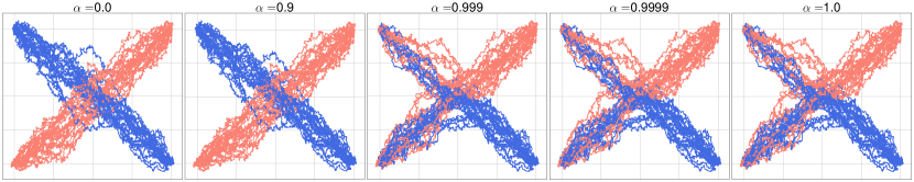
Figure 1: Influence of the augmentation on the bridge matching procedure in a toy example. In the training dataset the initial distribution corresponds to the Gaussian mixture with centers $(-2,-2)$ and $(-2,2)$. The terminal distribution corresponds to the Gaussian mixture with centers $(2,-2)$ and $(2,2)$. In the training dataset, the initial samples from the component with center $(-2,-2)$ are paired with the terminal ones from the component $(2,2)$ while the initial samples from the component with center $(-2,2)$ are paired with the terminal ones from the component $(2,-2)$. Each plot represents the learned coupling with a varying degree of augmentation ($\alpha=0$, augmented bridge matching and $\alpha=1$ original bridge matching, without augmentation). In blue we depict the trajectories arriving at the component $(2,-2)$ and in the red the ones arriving at $(2,2)$. While the training coupling is preserved for $\alpha=0$, its properties are lost as $\alpha$ increases from $0$ to $1$.

Notation. Given a probability space $\mathsf{X}$, we denote $\mathcal{P}(\mathsf{X})$ the space of probability measures on $\mathsf{X}$. We denote by $\mathcal{P}(\mathcal{C})$, the space of path measures, i.e. $\mathcal{P}(\mathcal{C})=\mathcal{P}(\mathrm{C}(\left[0,1\right],\mathbb{R}^{d}))$. The subset of Markov path measures associated with an SDE of the form $\mathrm{d}\mathbf{X}_{t}=v_{t}(\mathbf{X}_{t})\mathrm{d}t+\sigma_{t}\mathrm{d}\mathbf{B}_{t}$, with $\sigma,v$ locally Lipschitz, is denoted $\mathcal{M}$. For any $\mathbb{Q}\in\mathcal{M}$, we denote $\mathbb{Q}_{t}$ its marginal distribution at time $t$, $\mathbb{Q}_{s,t}$ the joint distribution at times $s$ and $t$, $\mathbb{Q}_{s|t}$ the conditional distribution at time $s$ given state at time $t$, and $\mathbb{Q}_{|0,1}\in\mathcal{P}(\mathcal{C})$ its diffusion bridge, i.e.  the distribution of $\mathbb{Q}$ conditioned on both endpoints. Unless specified otherwise, all gradient operators $\nabla$ are w.r.t. the variable $x_{t}$ with time index $t$. Let $(\mathsf{X},\mathcal{X})$ and $(\mathsf{Y},\mathcal{Y})$ be probability spaces. Given a Markov kernel $\mathrm{K}:\ \mathsf{X}\times\mathcal{Y}\to[0,1]$ and a probability measure $\mu$ defined on $\mathcal{X}$, we write $\mu\mathrm{K}$ the probability measure on $\mathcal{Y}$ such that for any $\mathsf{A}\in\mathcal{Y}$ we have $\mu\mathrm{K}(\mathsf{A})=\int_{\mathsf{X}}\mathrm{K}(x,\mathsf{A})\mathrm{d}\mu(x)$. In particular, for any joint distribution $\Pi_{0,1}\in\mathcal{P}(\mathbb{R}^{d}\times\mathbb{R}^{d})$, we denote the mixture of bridges measure as $\Pi=\Pi_{0,1}\mathbb{Q}_{|0,1}\in\mathcal{P}(\mathcal{C})$, which is short for $\Pi(\cdot)=\int_{\mathbb{R}^{d}\times\mathbb{R}^{d}}\mathbb{Q}_{|0,1}(\cdot|x_{0},x_{1})\Pi_{0,1}(\mathrm{d}x_{0},\mathrm{d}x_{1})$. For any measure $\Pi\in\mathcal{P}(\mathbb{R}^{d})$ we define the entropy of $\Pi$ has $\mathrm{H}(\Pi)=-\int_{\mathbb{R}^{d}}\log(\mathrm{d}\Pi/\mathrm{d}\lambda)(x)\mathrm{d}\Pi(x)$ if $\Pi$ admits a density w.r.t. the Lebesgue measure and $+\infty$ otherwise.

2 Background

Flow and Bridge matching.

We start by recalling some basics about bridge matching, see Lipman et al. (2022); Peluchetti (2021) for instance. We consider an initial coupling $\Pi_{0,1}$, i.e. a probability measure on $\mathbb{R}^{d}\times\mathbb{R}^{d}$. For example, in an imaging inverse problem, $\Pi_{0}$ represents the distribution of corrupted images and $\Pi_{1}$ the distribution of clean images. We also consider the path-measure $\mathbb{Q}$ associated with the Brownian motion $(\sigma\mathbf{B}_{t})_{t\in\left[0,1\right]}$, with $\sigma>0$. Practically, speaking, a sample from $\mathbb{Q}$ is a Brownian motion trajectory. We consider the path measure $\mathbb{P}=\Pi_{0,1}\mathbb{Q}_{|0,1}$. To sample from $\mathbb{P}$, first sample $(\mathbf{X}_{0},\mathbf{X}_{1})\sim\Pi_{0,1}$ and then sample a trajectory according to $\mathbb{Q}_{|0,1}(\cdot|(\mathbf{X}_{0},\mathbf{X}_{1}))$, i.e. sample a Brownian bridge interpolating between $\mathbf{X}_{0}$ and $\mathbf{X}_{1}$. For any $t\in\left[0,1\right]$ we have that $\mathbf{X}_{t}\sim\mathbb{P}_{t}$ with

$$\mathbf{X}_{t}=(1-t)\mathbf{X}_{0}+t\mathbf{X}_{1}+\sigma(t(1-t))^{1/2}\mathbf{Z},\qquad\mathbf{Z}\sim\mathrm{N}(0,\operatorname{Id}),\qquad(\mathbf{X}_{0},\mathbf{X}_{1})\sim\Pi_{0,1}.$$ (1)

This can also be expressed in a forward fashion with

$$\mathrm{d}\mathbf{X}_{t}=(\mathbf{X}_{1}-\mathbf{X}_{t})/(1-t)\mathrm{d}t+\sigma\mathrm{d}\mathbf{B}_{t},\qquad(\mathbf{X}_{0},\mathbf{X}_{1})\sim\Pi_{0,1}.$$ (2)

Note that the measure $\mathbb{P}$ is a priori non-Markovian. In Section 3, we will show that the measure is Markovian if and only if $\Pi_{0,1}$ is an entropic regularized Optimal Transport coupling between $\Pi_{0}$ and $\Pi_{1}$, i.e. a static Schrödinger Bridge. We are now ready to define the bridge matching measure $\mathbb{P}^{\star}$, associated with $(\mathbf{X}_{t}^{\star})_{t\in\left[0,1\right]}$ and given by

$$\mathrm{d}\mathbf{X}_{t}^{\star}=(\mathbb{E}_{\mathbb{P}_{1|t}}[\mathbf{X}_{1}]-\mathbf{X}_{t}^{\star})/(1-t)\mathrm{d}t+\sigma\mathrm{d}\mathbf{B}_{t},\qquad\mathbf{X}_{0}\sim\Pi_{0}.$$ (3)

The conditional expectation $\mathbb{E}_{\mathbb{P}_{1|t}}[\mathbf{X}_{1}]$ is estimated using that $\mathbb{E}_{\mathbb{P}_{1|t}}[\mathbf{X}_{1}]$ is the minimizer of a $\ell_{2}$ reconstruction loss. Note that in the case $\sigma=0$, the stochastic term vanishes and we recover the flow matching framework of Lipman et al. (2022). In practice, we train a neural network $\hat{x}_{1}^{\theta}$ to estimate $\mathbb{E}_{\mathbb{P}_{1|t}}[\mathbf{X}_{1}]$. The discrete Markov chain used at inference time is then obtained by discretizing $\mathrm{d}\mathbf{X}_{t}^{\star}=(\hat{x}_{1}^{\theta}(\mathbf{X}_{t})-\mathbf{X}_{t}^{\star})/(1-t)\mathrm{d}t+\sigma\mathrm{d}\mathbf{B}_{t}$ with $\mathbf{X}_{0}\sim\Pi_{0}$. The full training algorithm is recalled in Algorithm 1.

Algorithm 1 Bridge Matching

1:  Input: Joint distribution $\Pi_{0,1}$, Brownian bridge $\mathbb{Q}_{|0,1}$

2:  Let $\mathbb{P}=\Pi_{0,1}\mathbb{Q}_{|0,1}$.

3:  while not converged do

4:     Sample $(\mathbf{X}_{0},\mathbf{X}_{1})\sim\Pi_{0,1}$

5:     Sample $t\sim\mathrm{Unif}([0,1])$

6:     Sample $\mathbf{Z}\sim\mathrm{N}(0,\operatorname{Id})$

7:     Sample $\mathbf{X}_{t}=(1-t)\mathbf{X}_{0}+t\mathbf{X}_{1}+\sigma(t(1-t))^{1/2}\mathbf{Z}$

8:     ADAM step on $\|\hat{x}_{1}^{\theta}(\mathbf{X}_{t})-\mathbf{X}_{1}\|^{2}$

9:  end while

10:  Output: $\hat{x}_{1}^{\theta^{\star}}$

Schrödinger Bridges.

We briefly recall the concept of (static) Schrödinger bridge (Schrödinger, 1932). Given a path measure $\mathbb{Q}\in\mathcal{P}(\mathcal{C})$ and two distributions $\Pi_{0},\Pi_{1}\in\mathcal{P}(\mathbb{R}^{d})$, the static Schrödinger bridge is defined as

$$\Pi_{0,1}^{\star}=\operatorname*{arg\,min}\{\operatorname{KL}(\mu_{0,1}|\mathbb{Q}_{0,1})\,:\;\mu\in\mathcal{P}(\mathbb{R}^{d}\times\mathbb{R}^{d}),\ \mu_{0}=\Pi_{0},\ \mu_{1}=\Pi_{1}\}.$$ (4)

In other words, $\Pi^{\star}_{0,1}$ is the closest measure to $\mathbb{Q}_{0,1}$ w.r.t. the Kullback-Leibler divergence which satisfies the marginal constraints $\Pi_{0}$ and $\Pi_{1}$. In the case where $\mathbb{Q}$ is associated with $(\sigma\mathbf{B}_{t})_{t\in\left[0,1\right]}$ with $\sigma>0$, equation 4 can be rewritten as

$$\textstyle\Pi_{0,1}^{\star}=\operatorname*{arg\,min}\{\int\|x_{0}-x_{1}\|^{2}\mathrm{d}\mu(x_{0},x_{1})-(2\sigma^{2})\mathrm{H}(\mu)\,:\;\mu\in\mathcal{P}(\mathbb{R}^{d}\times\mathbb{R}^{d}),\ \mu_{0}=\Pi_{0},\ \mu_{1}=\Pi_{1}\},$$ (5)

where $\mathrm{H}$ is the entropy. Hence, in that setting, Schrödinger bridges coincide with the optimal coupling for the entropy regularized Wasserstein$-2$ distance. We refer to Peyré & Cuturi (2019) for more details on the links between Optimal Transport and Schrödinger Bridges. In our study we will show that the introduced augmented bridge matching procedure and the original bridge matching scheme coincide if and only if the training paired coupling is given by the static Schrödinger Bridge.

Doob $h$-transform.

The main theoretical tool of our analysis is the Doob $h$-transform (Palmowski & Rolski, 2002; Léonard, 2022). Assume that an initial path measure $\mathbb{P}$ can be represented as an SDE, then the Doob $h$-transform theory implies that some modification of $\mathbb{P}$ at the terminal end point can also be expressed using an SDE. More precisely, let $\mathbb{Q}\in\mathcal{P}(\mathrm{C}(\left[0,1\right],\mathbb{R}^{d}))$ be a path measure associated with $\mathrm{d}\mathbf{X}_{t}=b_{t}(\mathbf{X}_{t})\mathrm{d}t+\sigma_{t}\mathrm{d}\mathbf{B}_{t}$ with $b_{t}:\ \mathbb{R}^{d}\to\mathbb{R}^{d}$ and $\sigma_{t}\geq 0$. Next, given a potential function $h_{1}:\ \mathbb{R}^{d}\to\mathbb{R}_{+}$, we define $\mathbb{P}\in\mathcal{P}(\mathrm{C}(\left[0,1\right],\mathbb{R}^{d}))$ such that for any $\omega\in\mathrm{C}(\left[0,1\right],\mathbb{R}^{d})$

$$(\mathrm{d}\mathbb{P}/\mathrm{d}\mathbb{Q})(\omega)=h_{1}(\omega_{1}).$$ (6)

According to equation 6, $\mathbb{P}$ can be thought as a twisted version of $\mathbb{Q}$. We also define $h_{t}(x_{t})=\int_{\mathbb{R}^{d}}h_{1}(x_{1})\mathbb{Q}_{1|t}(\mathrm{d}x_{1},x_{t})$. Under mild assumptions on $h_{1}$, $\mathbb{P}$ is also associated with an SDE, see (Palmowski & Rolski, 2002, Lemma 3.1), which we recall in the following proposition.

Proposition .

Assume that $h\in\mathrm{C}^{2}(\left[0,1\right]\times\mathbb{R}^{d},\mathbb{R}_{+})$ is bounded and that $(t,x)\mapsto\langle b_{t}(x),\nabla h_{t}(x)\rangle+(\sigma_{t}^{2}/2)\Delta h_{t}(x)$ is measurable and bounded. Assume that $\inf\{h_{t}(x)\,:\;x\in\mathbb{R}^{d},t\in\left[0,1\right]\}>0$. Then, $\mathbb{P}$ is associated with $\mathrm{d}\mathbf{X}_{t}=\{b_{t}(\mathbf{X}_{t})+\sigma_{t}^{2}\nabla\log h_{t}(\mathbf{X}_{t})\}\mathrm{d}t+\sigma_{t}\mathrm{d}\mathbf{B}_{t}$.

This result will be key to establish the SDE representation of mixture of bridges and to derive the augmented bridge matching procedure. In particular, using Section 2, we have that if $\nabla\log h_{t}$ is available, then one can sample from $\mathbb{P}$, the twisted version $\mathbb{Q}$, by first sampling $\mathbf{X}_{0}\sim\mathbb{P}_{0}$ and then discretizing the dynamics given by $\mathrm{d}\mathbf{X}_{t}=\{b_{t}(\mathbf{X}_{t})+\sigma_{t}^{2}\nabla\log h_{t}(\mathbf{X}_{t})\}\mathrm{d}t+\sigma_{t}\mathrm{d}\mathbf{B}_{t}$.

3 Augmented Bridge Matching

In this section, we first show that the fixed points of the bridge matching procedure are necessarily Schrödinger bridges. Then, we introduce Augmented Bridge Matching, a simple modification of Bridge Matching which ensures that couplings are preserved. As in Liu et al. (2023); Somnath et al. (2023), we consider a paired setting with a coupling $\Pi_{0,1}\in\mathcal{P}(\mathbb{R}^{d}\times\mathbb{R}^{d})$. We aim at deriving a SDE representation of $\mathbb{P}=\Pi_{0,1}\mathbb{Q}_{|0,1}$, where $\mathbb{Q}_{|0,1}$ is a given bridge, usually a Brownian bridge. In what follows, we assume that $\mathbb{Q}$ is associated with $\mathrm{d}\mathbf{X}_{t}=b_{t}(\mathbf{X}_{t})\mathrm{d}t+\sigma_{t}\mathrm{d}\mathbf{B}_{t}$ with $b:\ \left[0,1\right]\times\mathbb{R}^{d}\to\mathbb{R}^{d}$ and $\sigma:\ [0,1]\to(0,+\infty)$. We recover the Brownian case if $b=0$ and $\sigma_{t}=\sigma>0$.

Fixed points of bridge matching.

In the next proposition, we provide necessary and sufficient conditions under which the coupling is preserved when considering bridge matching. More precisely, we consider $(\mathbf{X}_{t}^{\mathcal{M}})_{t\in\left[0,1\right]}$ given by

$$\textstyle\mathrm{d}\mathbf{X}_{t}^{\mathcal{M}}=\{b_{t}(\mathbf{X}_{t}^{\mathcal{M}})+\sigma_{t}^{2}\mathbb{E}_{\mathbb{P}_{1|t}}[\nabla\log\mathbb{Q}_{1|t}(\mathbf{X}_{1}^{\mathcal{M}}|\mathbf{X}_{t}^{\mathcal{M}})\ |\ \mathbf{X}_{t}^{\mathcal{M}}]\}\mathrm{d}t+\sigma_{t}\mathrm{d}\mathbf{B}_{t},\quad\mathbf{X}_{0}^{\mathcal{M}}\sim\Pi_{0}.$$ (7)

Importantly, note that in the case where $\mathbb{Q}$ is associated with $(\sigma\mathbf{B}_{t})_{t\in\left[0,1\right]}$ then $(\mathbf{X}_{t}^{\mathcal{M}})_{t\in\left[0,1\right]}$ coincides with $(\mathbf{X}_{t}^{\star})_{t\in\left[0,1\right]}$ in Section 2. In particular, equation 7 is a generalization of the bridge matching procedure considered in Peluchetti (2021); Liu et al. (2023); Somnath et al. (2023); Lipman et al. (2022), see Shi et al. (2023) for a study of such bridges. We denote by $\mathbb{P}^{\mathcal{M}}$ the (Markov) path measure associated with equation 7. We recall that the (static) Schrödinger Bridge $\Pi_{0,1}^{\star}$ is given by equation 4. The next proposition is our main result.

Proposition .

Under mild assumptions on $\Pi$ and $\mathbb{Q}$, $\mathbb{P}^{\mathcal{M}}_{0,1}=\Pi_{0,1}$ if and only if $\Pi_{0,1}=\Pi_{0,1}^{\star}$.

In other words, Section 3 shows that the bridge matching procedure preserves the coupling if and only if the original coupling used for training is the static Schrödinger Bridge. In Somnath et al. (2023); Liu et al. (2023), it remains debatable whether the training dataset pairs $\{(X_{0}^{i},X_{1}^{i})\}_{i=1}^{N}$ inherently represent the solution to the static Schrödinger Bridge equation 4. In particular, this assumption is not ensured in real-world applications and can be easily violated even in low-dimensional cases as shown in Figure 1. Hence, the bridge matching procedure does not preserve the original coupling in general.

Comparison between stochastic and deterministic matching.

One key assumption of Section 3 is that $\sigma>0$. In the case $\sigma=0$, we recover the flow matching procedure (Lipman et al., 2022), which is the deterministic counterpart of bridge matching. The fixed points of flow matching have been investigated in Liu et al. (2022b); Liu (2022). In particular, it is shown in Liu et al. (2022b) that any straight coupling is a fixed point of flow matching. In particular it can be shown that there exists straight couplings which are not optimal coupling for any convex cost (Liu, 2022, Example 3.5). In contrast, Section 3 ensures that fixed points of bridge matching are always optimal couplings. This is a key difference between the deterministic and the stochastic setting. More precisely, by introducing stochasticity into the original process we can obtain the uniqueness of the fixed point of the bridge matching, which is not the case in the deterministic setting (flow matching).

Augmented Bridge Matching.

We are now ready to introduce the Augmented Bridge Matching procedure. We recall that $\mathbb{P}=\Pi_{0,1}\mathbb{Q}_{|0,1}$, where $\Pi_{0,1}$ is the original training coupling and $\mathbb{Q}$ is associated with

$$\mathrm{d}\mathbf{X}_{t}=b_{t}(\mathbf{X}_{t})\mathrm{d}t+\sigma_{t}\mathrm{d}\mathbf{B}_{t},\qquad\mathbf{X}_{0}\sim\mathbb{Q}_{0}.$$ (8)

We define $h_{1}:\ \mathbb{R}^{d}\times\mathbb{R}^{d}\to\mathbb{R}_{+}$ given for any $x_{0},x_{1}$ by $h_{1}(x_{0},x_{1})=(\mathrm{d}\mathbb{P}_{1|0}/\mathrm{d}\mathbb{Q}_{1|0})(x_{0},x_{1})$. Similarly, as in Section 2, we define for any $t\in\left[0,1\right]$ and $x_{0},x_{t}\in\mathbb{R}^{d}$, $h_{t}(x_{0},x_{t})=\int_{\mathbb{R}^{d}}h_{1}(x_{0},x_{1})\mathbb{Q}_{1|t}(\mathrm{d}x_{1},x_{t})$. We have the following result, which is a direct consequence of Doob’s $h$-transform. The full proof is postponed to Appendix C.

Proposition .

Assume that for any $x_{0}\in\mathbb{R}^{d}$, $h(x_{0},\cdot)$ satisfies the conditions of Section 2. Then, $\mathbb{P}$ is associated with

$$\textstyle\mathrm{d}\mathbf{X}_{t}=\{b_{t}(\mathbf{X}_{t})+\sigma_{t}^{2}\mathbb{E}_{\mathbb{P}_{1|0,t}}[\nabla\log\mathbb{Q}_{1|t}(\mathbf{X}_{1}|\mathbf{X}_{t})\ |\ \mathbf{X}_{0},\mathbf{X}_{t}]\}\mathrm{d}t+\sigma_{t}\mathrm{d}\mathbf{B}_{t},\quad\mathbf{X}_{0}\sim\Pi_{0}.$$ (9)

In particular, $(\mathbf{X}_{0},\mathbf{X}_{1})\sim\Pi_{0,1}$.

Proof.

In what follows, we give an outline of the proof. We fix $x_{0}\in\mathbb{R}^{d}$ and for any $\omega\in\mathrm{C}(\left[0,1\right],\mathbb{R}^{d})$ we have $\mathrm{d}\mathbb{P}_{|0}(\omega|x_{0})=\mathrm{d}\mathbb{Q}_{|0}(\omega|x_{0})(\mathrm{d}\mathbb{P}_{1|0}/\mathrm{d}\mathbb{Q}_{1|0})(\omega_{1},x_{0})$. Then, using Section 2 we obtain that $\mathbb{P}_{|0}(\cdot,x_{0})$ is associated with

$$\textstyle\mathrm{d}\mathbf{X}_{t}=\{b_{t}(\mathbf{X}_{t})+\sigma_{t}^{2}\nabla\log h_{t}(\mathbf{X}_{t},x_{0})\}\mathrm{d}t+\sigma_{t}\mathrm{d}\mathbf{B}_{t}.$$ (10)

Finally, we remark that for any $t\in\left[0,1\right]$ and $x_{0},x_{t}\in\mathbb{R}^{d}$ we have

$$\textstyle\nabla\log h_{t}(x_{t},x_{0})\textstyle=\int_{\mathbb{R}^{d}}\tfrac{\mathbb{P}_{1|0}(x_{1}|x_{0})\mathbb{Q}_{1|t}(x_{1}|x_{t})}{\mathbb{Q}_{1|0}(x_{1}|x_{0})h_{t}(x_{t}|x_{0})}\nabla\log\mathbb{Q}_{1|t}(x_{1}|x_{t})\mathrm{d}x_{1}$$ (11)

$$\qquad\textstyle=\int_{\mathbb{R}^{d}}\tfrac{\mathbb{P}_{1|0}(x_{1}|x_{0})\mathbb{Q}_{t|0,1}(x_{t}|x_{0},x_{1})}{\mathbb{Q}_{t|0}(x_{t}|x_{0})h_{t}(x_{t}|x_{0})}\nabla\log\mathbb{Q}_{1|t}(x_{1}|x_{t})\mathrm{d}x_{1}$$ (12)

$$\qquad\textstyle=\int_{\mathbb{R}^{d}}\tfrac{\mathbb{P}_{t,1|0}(x_{t},x_{1}|x_{0})}{\mathbb{P}_{t|0}(x_{t}|x_{0})}\nabla\log\mathbb{Q}_{1|t}(x_{1}|x_{t})\mathrm{d}x_{1}=\textstyle\int_{\mathbb{R}^{d}}\nabla\log\mathbb{Q}_{1|t}(x_{1}|x_{t})\mathbb{P}_{1|t,0}(x_{1}|x_{t},x_{0})\mathrm{d}x_{1},$$ (13)

where the first equality is obtained using the definition of $h_{t}$, the second using the key relationship that $\mathbb{Q}_{1|t}\mathbb{Q}_{t|0}=\mathbb{Q}_{t|0,1}\mathbb{Q}_{1|0}$ and the third using the definition of $\mathbb{P}$ and that $\mathbb{P}_{t|0}=\mathbb{Q}_{t|0}h_{t}$. The last equality follows from Bayes’ rule. ∎

This suggests the following algorithm to approximately sample from $\Pi_{0,1}$: first sample $\mathbf{X}_{0}\sim\Pi_{0}$ and then sample $(\mathbf{X}_{t})_{t\in\left[0,1\right]}$ according to equation 10. The term $\int_{\mathbb{R}^{d}}\nabla\log\mathbb{Q}_{1|t}(x_{1}|\mathbf{X}_{t})\mathrm{d}\mathbb{P}_{1|0,t}(x_{1},(\mathbf{X}_{0},\mathbf{X}_{t}))$ is not tractable and is approximated by $v_{t}^{\theta}$ minimizing the following loss function

$$\textstyle\mathcal{L}(\theta)=\int_{0}^{1}\lambda_{t}\mathbb{E}[\|v_{t}^{\theta}(\mathbf{X}_{0},\mathbf{X}_{t})-\nabla\log\mathbb{Q}_{1|t}(\mathbf{X}_{1}|\mathbf{X}_{t})\|^{2}]\mathrm{d}\mathbb{P}(\mathbf{X}_{0},\mathbf{X}_{t},\mathbf{X}_{1}),$$ (14)

where $(\lambda_{t})_{t\in\left[0,1\right]}$ is a weighting function. The full algorithm is given in Algorithm 2.

Algorithm 2 Augmented Bridge Matching (AugBM)

1:  Input: Joint distribution $\Pi_{0,1}$, Brownian bridge $\mathbb{Q}_{|0,1}$

2:  Let $\mathbb{P}=\Pi_{0,1}\mathbb{Q}_{|0,1}$.

3:  while not converged do

4:     Sample $(\mathbf{X}_{0},\mathbf{X}_{1})\sim\Pi_{0,1}$

5:     Sample $t\sim\mathrm{Unif}([0,1])$

6:     Sample $\mathbf{Z}\sim\mathrm{N}(0,\operatorname{Id})$

7:     Sample $\mathbf{X}_{t}=(1-t)\mathbf{X}_{0}+t\mathbf{X}_{1}+\sigma(t(1-t))^{1/2}\mathbf{Z}$

8:     ADAM step on $\|\hat{x}_{1}^{\theta}(\mathbf{X}_{0},\mathbf{X}_{t})-\mathbf{X}_{1}\|^{2}$

9:  end while

10:  Output: $x_{1}^{\theta^{\star}}$

Comparison with bridge matching.

The algorithm described in Algorithm 2 closely resembles the ones proposed in Liu et al. (2023); Somnath et al. (2023), see Algorithm 1. However, the main difference (highlighted in red) is that the velocity field $v_{t}$ can depends on $x_{0}$ in our case. Doing so, we do not get that $(\mathbf{X}_{t})_{t\in\left[0,1\right]}$ is Markovian as it depends on the initial condition $\mathbf{X}_{0}$. However, in Liu et al. (2023); Somnath et al. (2023), the coupling $\Pi_{0,1}$ is provably not preserved by $(\mathbf{X}_{t})_{t\in\left[0,1\right]}$.

Therefore in Augmented Bridge Matching the drift depends on both $\mathbf{X}_{0}$ and $\mathbf{X}_{t}$, i.e. the dynamics is not Markovian, but the coupling is preserved. In the original bridge matching procedure, the drift only depends on $\mathbf{X}_{t}$ and the coupling is not preserved, as we have seen in Section 3. It is also possible to interpolate between the fully augmented bridge matching procedure and the original bridge matching by conditioning the velocity field on $\mathbf{X}_{\alpha t}$. If $\alpha=0$ we recover the augmented bridge matching while for $\alpha=1$ we recover the original scheme. The effect of $\alpha$ on the preservation of the original coupling is illustrated in Figure 1.

4 Bridge matching and diffusion model based interpolation

Finally, in this section, we show that the bridge matching procedure can be shown to be equivalent to a methodology based on diffusion models. We start by recalling the method introduced in Zhou et al. (2023), which leverages the framework of diffusion models to propose an interpolation procedure.

Denoising Diffusion Bridge Models.

As in the previous section, we consider a paired setting with a coupling $\Pi_{0,1}\in\mathcal{P}(\mathbb{R}^{d}\times\mathbb{R}^{d})$. We aim at deriving a SDE representation of $\mathbb{P}=\Pi_{0,1}\mathbb{Q}_{|0,1}$. First, consider the forward noising process given by $\mathbb{P}_{|1}(\cdot|x_{1})=\Pi_{0|1}\mathbb{Q}_{|0,1}(\cdot|x_{1})$ for an arbitrary $x_{1}\in\mathbb{R}^{d}$. This forward noising process is associated with

$$\mathrm{d}\mathbf{X}_{t}=\{b_{t}(\mathbf{X}_{t})+\sigma_{t}^{2}\nabla\log\mathbb{Q}_{1|t}(x_{1}|\mathbf{X}_{t})\}\mathrm{d}t+\sigma_{t}\mathrm{d}\mathbf{B}_{t},\qquad\mathbf{X}_{0}\sim\Pi_{0|1}.$$ (15)

This forward representation is associated with a backward one, $(\mathbf{Y}_{1-t})_{t\in\left[0,1\right]}=(\mathbf{X}_{t})_{t\in\left[0,1\right]}$ where

$$\mathrm{d}\mathbf{Y}_{t}=\{-b_{1-t}(\mathbf{Y}_{t})-\sigma_{1-t}^{2}\nabla\log\mathbb{Q}_{1|1-t}(\mathbf{Y}_{1}|\mathbf{Y}_{t})+\sigma_{1-t}^{2}\nabla\log\mathbb{P}_{1-t|1}(\mathbf{Y}_{t}|\mathbf{Y}_{1})\}\mathrm{d}t+\sigma_{1-t}\mathrm{d}\mathbf{B}_{t}.$$ (16)

If we consider $(\mathbf{Y}_{t})_{t\in\left[0,1\right]}$ such that $\mathbf{Y}_{1}\sim\Pi_{1}$ and $(\mathbf{Y}_{t})_{t\in\left[0,1\right]}$ satisfies equation 16, then we have that $(\mathbf{Y}_{t})_{t\in\left[0,1\right]}\sim\Pi_{1}\mathbb{P}_{|1}=\Pi_{0,1}\mathbb{Q}_{|0,1}$. Hence, we have that $(\mathbf{Y}_{t})_{t\in\left[0,1\right]}\sim\mathbb{P}$ and in particular the coupling is preserved, i.e. $(\mathbf{Y}_{0},\mathbf{Y}_{1})\sim\Pi_{0,1}$ as in Augmented Bridge Matching. While $\nabla\log\mathbb{Q}_{1|1-t}$ is tractable, $\nabla\log\mathbb{P}_{1-t|1}$ is not and needs to be approximated. However, it can be shown that

$$\textstyle\nabla\log\mathbb{P}_{1-t|1}(x_{1-t}|x_{1})=\int_{\mathbb{R}^{d}}\nabla\log\mathbb{Q}_{1-t|0,1}(x_{1-t}|x_{0},x_{1})\mathrm{d}\mathbb{P}_{0|1-t,1}(x_{0}|x_{1-t},x_{1}).$$ (17)

Hence, we get that

$$\textstyle\nabla\log\mathbb{P}_{t|1}(x_{t}|x_{1})=\operatorname*{arg\,min}_{s}\mathbb{E}_{\Pi_{0,1}\mathbb{Q}_{t|0,1}}[\|s(t,\mathbf{X}_{t},\mathbf{X}_{1})-\nabla\log\mathbb{Q}_{t|0,1}(\mathbf{X}_{t}|\mathbf{X}_{0},\mathbf{X}_{1})\|^{2}],$$ (18)

which can be approximately computed since $\mathbb{Q}_{t|0,1}$ is tractable, see (Zhou et al., 2023, Theorem 1). At inference time, Zhou et al. (2023) sample from $\Pi_{1}$ and compute $(\mathbf{Y}_{t})_{t\in\left[0,1\right]}$ using equation 16 and the score approximation.

Unifying the models.

We now show that DDBM is equivalent to the augmented bridge matching procedure we propose. By definition $\mathbb{Q}$ is associated with $\mathrm{d}\mathbf{X}_{t}=b_{t}(\mathbf{X}_{t})\mathrm{d}t+\sigma_{t}\mathrm{d}\mathbf{B}_{t}$ and $\mathbf{X}_{0}\sim\mathbb{Q}_{0}$, see equation 8. Using the time-reversal formula, we get that $\mathbb{Q}$ is also associated with $(\mathbf{Y}_{1-t})_{t\in\left[0,1\right]}$ such that

$$\mathrm{d}\mathbf{Y}_{t}=\{-b_{1-t}(\mathbf{Y}_{t})+\sigma_{1-t}^{2}\nabla\log\mathbb{Q}_{1-t}(\mathbf{Y}_{t})\}\mathrm{d}t+\sigma_{t}\mathrm{d}\mathbf{B}_{t},\qquad\mathbf{Y}_{1}\sim\mathbb{Q}_{1}.$$ (19)

Therefore, in order to sample from $\Pi_{1}\mathbb{Q}_{|1}$, first sample $\mathbf{Y}_{1}\sim\Pi_{1}$ and then sample $(\mathbf{Y}_{t})_{t\in\left[0,1\right]}$ according to equation 19. Next, we apply Section 3 with $b_{t}$ replaced $-b_{1-t}+\sigma_{1-t}^{2}\nabla\log\mathbb{Q}_{1-t}$, and $\Pi_{0}$ replaced by $\Pi_{1}$. The augmented bridge matching procedure of Section 3 is given by $\mathbf{Y}_{0}\sim\Pi_{1}$ and

$$\textstyle\mathrm{d}\mathbf{Y}_{t}=\{-b_{1-t}(\mathbf{X}_{t})+\sigma_{1-t}^{2}\nabla\log\mathbb{Q}_{1-t}(\mathbf{Y}_{t})$$ (20)

$$\qquad\qquad\qquad+\sigma_{1-t}^{2}\mathbb{E}_{\mathbb{P}_{0|1,1-t}}[\nabla\log\mathbb{Q}_{0|1-t}(\mathbf{Y}_{1}|\mathbf{Y}_{0})\ |\ \mathbf{Y}_{0},\mathbf{Y}_{t}])\}\mathrm{d}t+\sigma_{1-t}\mathrm{d}\mathbf{B}_{t}.$$ (21)

The next proposition shows that equation 20 and equation 16 are the same SDEs.

Proposition .

For any $t\in\left[0,1\right]$ we have $\nabla\log\mathbb{Q}_{t}+\mathbb{E}_{\mathbb{P}_{0|1,t}}[\nabla\log\mathbb{Q}_{0|t}]=\nabla\log\mathbb{P}_{t|1}-\nabla\log\mathbb{Q}_{1|t}$.

Combining Section 4, equation 20 and equation 16 and we can conclude that DDBM is an augmented bridge matching procedure for the time-reversed SDE, i.e. the two methods coincide if we invert the roles of $\Pi_{0}$ and $\Pi_{1}$ and the arrow of time.

5 Related work

Bridge matching.

Bridge matching was first introduced by Peluchetti (2021). It has recently been applied to high dimensional settings in Liu et al. (2023); Somnath et al. (2023); Delbracio & Milanfar (2023); Tong et al. (2023); Albergo et al. (2023); Albergo & Vanden-Eijnden (2022); Pooladian et al. (2023). The deterministic counterpart to this procedure was first introduced in Lipman et al. (2022) and named flow matching, see also Heitz et al. (2023). These approaches first sample both the initial and terminal point according to a coupling, i.e. they assume access to a paired dataset (which might be given by the independent coupling). Then, they consider an interpolation between these two samples using a Brownian bridge (or a linear interpolation in the case of Lipman et al. (2022)). Finally, they learn a drift (or velocity field) which best approximates this non-Markovian dynamics. It turns out that this procedure is the Markovian projection (Gyöngy, 1986) which has been studied in finance. We note that it is possible to extend this procedure to the case where only unpaired datasets are available has been considered in using iterative procedure and tools from Optimal Transport (Liu et al., 2022b; Liu, 2022; Shi et al., 2023; Peluchetti, 2023; Tong et al., 2023).

Diffusion Schrödinger Bridge.

The theoretical properties of Schrödinger Bridges (Schrödinger, 1932) have been extensively investigated using tools from probability and stochastic control theory (Léonard, 2014; Dai Pra, 1991; Chen et al., 2021b). In the context of machine learning, the Diffusion Schrödinger Bridge algorithm was introduced in De Bortoli et al. (2021); Vargas et al. (2021); Chen et al. (2021a). These methods have been extended to solve conditional simulation and more general control problems (Shi et al., 2022; Thornton et al., 2022; Liu et al., 2022a; Tamir et al., 2023). Recently Shi et al. (2023); Peluchetti (2023) have introduced a new iterative methodology to solve Schrödinger bridges based on Markovian and reciprocal class projections.

Doob $h$-transform.

The Doob $h$-transform is an ubiquitous tool in probability theory (Palmowski & Rolski, 2002; Rogers & Williams, 2000; Chung & Walsh, 2006). In the context of diffusion models it has been leveraged in Heng et al. (2021); Liu et al. (2022c) to learn bridges. Recently, machine learning approaches have also been proposed to learn Doob $h$-transforms in the context of sampling (Chopin et al., 2023).

6 Experiments

In Section 6.1 we first empirically verify that the Schrödinger Bridge is the only fixed point of the bridge matching procedure in a Gaussian setting. In Section 6.2, we illustrate the efficiency of the augmented bridge matching procedure in a multi-domain image-to-image translation setting.

6.1 Toy experiment

First, we illustrate Section 3 in a simple Gaussian setting. We consider the case where $\Pi_{0}=\Pi_{1}=\mathrm{N}(0,1)$. We assume that $\mathbb{P}_{0,1}=\mathrm{N}(0,\Sigma^{\alpha})$, with $\Sigma^{\alpha}\in\mathbb{R}^{d\times d}$ symmetric with $\Sigma^{\alpha}_{0,0}=\Sigma^{\alpha}_{1,1}=1$ and $\Sigma^{\alpha}_{0,1}=\alpha$ with $\alpha\in\left(0,1\right)$. We consider $\mathbb{Q}$ associated with $(\sigma\mathbf{B}_{t})_{t\in\left[0,1\right]}$. We have the following result.

Proposition .

The static Schrödinger Bridge $\Pi_{0,1}^{\star}$, solution of equation 4 is given by $\Pi^{\star}_{0,1}=\mathrm{N}(0,\Sigma^{\star})$ with $\Sigma^{\star}=\Sigma^{\alpha^{\star}}$ with $\alpha^{\star}=(\sigma^{2}/2)(\sqrt{1+4/\sigma^{4}}-1)$. In addition, for any $\alpha\in\left(0,1\right)$ and $\Pi_{0,1}=\mathrm{N}(0,\Sigma^{\alpha})$, we get that $\mathbb{P}_{0,1}^{\mathcal{M}}=\mathrm{N}(0,\Sigma^{f(\alpha)})$ with $f$ explicit and given in the appendix.

Finally, in Figure 2, we empirically illustrate that $f(\alpha)=\alpha$, i.e. $\Pi_{0,1}=\mathbb{P}_{0,1}^{\mathcal{M}}$ only if $\alpha=\alpha^{\star}$ for different values of $\sigma$. This means that, even in this simplified Gaussian setting, the Markovian projection only preserves the coupling if and only if $\Pi_{0,1}$ is the Schrödinger Bridge.

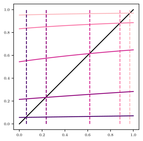
Figure 2: $f(\alpha)$ as a function of $\alpha$ for $\sigma\in\{0.25,0.5,1.,2.\}$ (dark to clear). Vertical lines correspond to the value of $\alpha^{\star}$ for the corresponding value of $\sigma$. Note that $f(\alpha)=\alpha$ if and only if $\alpha=\alpha^{\star}$, i.e. the coupling is preserved if and only if the original coupling is the Schrödinger Bridge.

6.2 Multi-domain image-to-image translation

Next, we test out our AugBM on multi-domain image-to-image translation. Our goal is to train a single diffusion model with versatile capabilities, enabling it to perform translations across multiple domains. Specifically, we consider two popular image-to-image translation tasks from pix2pix (Isola et al., 2017), namely edges2shoes and edges2handbags, and the colorization task on ImageNet dataset. For each task, we train an AugBM to transfer between two provided domains in a bidirectional manner, without prior knowledge of which domain is in focus. We compare our AugBM mainly to I²SB (Liu et al., 2023), which can be viewed as the special case of our AugBM without augmentation. To ensure a fair comparison, we adopt the same setup from I²SB, where we parametrize $\hat{x}_{1}^{\theta}$ using a U-Net (Ronneberger et al., 2015) initialized with the unconditional ADM checkpoint (Dhariwal & Nichol, 2021). We maintain consistency across all training hyperparameters to ensure that any observed performance disparities are solely attributed to the algorithmic distinctions between the models. All images are in 256$\times$256 resolution.

Figure 4 reports the qualitative results, which encompass both the generation processes (in the odd rows) and the predicted couplings (in the even rows), i.e., $\mathbf{X}_{T}^{\varepsilon}$. It’s worth noting a significant deviation in the generation processes between the two models beyond the midpoint, i.e., after $t\geq 0.5$. In the case of our AugBM, it effectively transports samples to their correct target domains. In contrast, I²SB tends to return them to their original source, effectively recreating the same source image. Indeed, for bidirectional translation tasks, it is extremely difficult to determine the target direction based merely on the intermediate samples, especially at the midpoint, without additional information, such as the augmentation utilized in AugBM.

It is essential to note that, in such cases, both models preserve the marginal, but only our AugBM preserves the coupling. Figure 4 provides quantitative demonstration, where we report the Frechet Inception Distance (FID; (Heusel et al., 2017)) w.r.t. the joint domain as a measure of marginal, and the averaged FID w.r.t. individual domains—as a measure of coupling. All FID values are computed w.r.t. the validation statistics. Although both models manage to achieve low marginal FIDs (with AugBM maintaining a performance advantage), our AugBM surpasses I²SB when it comes to coupling FIDs, particularly in scenarios with high number of function evaluation (NFE) regimes.

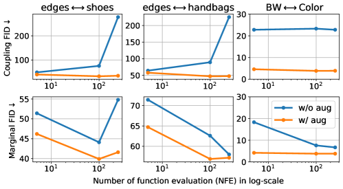
Figure 3: Qualitative results between our augmented bridge matching (2${}^{\text{nd}}$-5${}^{\text{th}}$ columns) and standard bridge matching (6${}^{\text{th}}$-9${}^{\text{th}}$ columns). We include both the generation trajectories, $\mathbf{X}_{t}$, and the predicted coupling, $\mathbf{X}_{T}^{\varepsilon}$, at different time steps.

Figure 4: Quantitative results between standard bridge matching (marked blue) and our augmented bridge matching (marked orange). We report three pix2pix (Isola et al., 2017) datasets in each column. It is clear that our augmented bridge matching not only preserve the coupling (first row), but also yields better marginal (second row).

7 Discussion

In this work, we introduce Augmented Bridge Matching, a simple modification of the original Bridge Matching methodology which relaxes the Markovian property and preserves the original training coupling. One of our main contribution is to clarify what properties are preserved by the bridge matching procedure. In particular, we show that the training coupling is preserved if and only if it is given by the optimal transport coupling. Our main conclusion is that if the pairing properties of the training dataset are of importance then one should use augmented bridge matching.

Several methodological challenges remain to be addressed. First, while we have proposed a smooth interpolation between the original bridge matching and the augmented bridge matching, i.e. by conditioning on $\mathbf{X}_{\alpha t}$ with $\alpha\in\left[0,1\right]$, it is not clear which properties are preserved if $\alpha\in(0,1)$. In practice the loss of the Markovian property and the extra conditioning might make the training more difficult by increasing the variance of the loss. This is especially true if the training coupling is highly entropic, as illustrated in Appendix E. In future work, we will further investigate the interaction between the loss variance and the entropy of the training coupling.

Organization of the appendix

In Appendix A, we recall some basics of stochastic calculus. In Appendix B, we prove Section 3. In Appendix C, we prove Section 3. We complement Section 3 with an in-depth study of the Gaussian case in Appendix D. Additional image examples are presented in Appendix F.

Appendix A Basics of stochastic calculus

We start by recalling some useful definitions from stochastic calculus.

Definition (Infinitesimal generator).

An operator $\mathcal{A}$ is an infinitesimal generator if there exists $b$ measurable such that for any $\varphi\in\mathrm{C}_{c}^{2}(\mathbb{R}^{d})$, $t\in\left[0,1\right]$ and $x\in\mathbb{R}^{d}$

$$\mathcal{A}_{t}(\varphi)(x)=\langle b_{t}(x),\nabla\varphi(x)\rangle+(1/2)\Delta\varphi(x).$$ (22)

Equipped with the definition of infinitesimal generator, we define solutions to martingale problem.

Definition (Martingale solution).

We say that a path measure $\mathbb{P}\in\mathcal{P}(\mathrm{C}(\left[0,1\right],\mathbb{R}^{d}))$ is a solution to a martingale problem with infinitesimal generator $\mathcal{A}$ if for any $\varphi\in\mathrm{C}_{c}^{2}(\mathbb{R}^{d})$, $u(\mathbf{X}_{t})-\int_{0}^{t}\mathcal{A}_{s}(\varphi)(\mathbf{X}_{s})\mathrm{d}s$ is a local $\mathbb{P}$-martingale.

In Section 2, we say that $\mathbb{P}\in\mathcal{P}(\mathrm{C}(\left[0,1\right],\mathbb{R}^{d})$ is associated with $\mathrm{d}\mathbf{X}_{t}=b_{t}(\mathbf{X}_{t})\mathrm{d}t+\mathrm{d}\mathbf{B}_{t}$ if $\mathbb{P}$ is a solution to the martingale problem with infinitesimal generator equation 22. We refer to Stroock & Varadhan (2007) for more details about the notion of martingale problem.

Appendix B Proof of Section 3

We recall that $\mathbb{P}=\Pi_{0,1}\mathbb{Q}_{|0,1}$, where $\mathbb{Q}_{|0,1}$ is a given bridge, usually a Brownian bridge. In what follows, we assume that $\mathbb{Q}$ is associated with $\mathrm{d}\mathbf{X}_{t}=b_{t}(\mathbf{X}_{t})\mathrm{d}t+\sigma_{t}\mathrm{d}\mathbf{B}_{t}$ with $b:\ \left[0,1\right]\times\mathbb{R}^{d}\to\mathbb{R}^{d}$ and $\sigma:\ [0,1]\to(0,+\infty)$. We recover the Brownian case if $b=0$ and $\sigma_{t}=\sigma>0$. We recall that the Markovian projection $\mathbb{P}^{\mathcal{M}}$ is associated with

$$\textstyle\mathrm{d}\mathbf{X}_{t}^{\mathcal{M}}=\{b_{t}(\mathbf{X}_{t}^{\mathcal{M}})+\sigma_{t}^{2}\mathbb{E}_{\mathbb{P}_{1|t}}[\nabla\log\mathbb{Q}_{1|t}(\mathbf{X}_{1}^{\mathcal{M}}|\mathbf{X}_{t}^{\mathcal{M}})\ |\ \mathbf{X}_{t}^{\mathcal{M}}]\}\mathrm{d}t+\sigma_{t}\mathrm{d}\mathbf{B}_{t},\quad\mathbf{X}_{0}^{\mathcal{M}}\sim\Pi_{0}.$$ (23)

We also consider the following assumptions.

A 1.

$(t,x_{t})\mapsto\mathbb{E}_{\Pi_{1|t}}[\nabla\log\mathbb{Q}_{1|t}(\mathbf{X}_{1}|\mathbf{X}_{t})\ |\ \mathbf{X}_{t}=x_{t}]$ are locally Lipschitz and there exist $C>0$, $\psi\in\mathrm{C}(\left[0,1\right],\mathbb{R}_{+})$ such that for any $t\in\left[0,1\right]$ and $x_{0},x_{t}\in\mathbb{R}^{d}$, we have

$$\|\mathbb{E}_{\Pi_{1|t}}[\nabla\log\mathbb{Q}_{1|t}(\mathbf{X}_{1}|\mathbf{X}_{t})\ |\ \mathbf{X}_{t}=x_{t}]\|\leq C\psi(t)(1+\|x_{t}\|).$$ (24)

In addition, we consider the following assumption ensuring that the Doob $h$-transform is well-defined.

A 2.

For any $x_{0}\in\mathbb{R}^{d}$, $\Pi_{1|0}$ is absolutely continuous w.r.t. $\mathbb{Q}_{1|0}$. For any $x_{0}\in\mathbb{R}^{d}$, let $\varphi_{1|0}$ be given for any $x_{1}\in\mathbb{R}^{d}$ by $\varphi_{1|0}(x_{1}|x_{0})=\mathrm{d}\Pi_{1|0}(x_{1}|x_{0})/\mathrm{d}\mathbb{Q}_{1|0}(x_{1}|x_{0})$ and assume that for any $x_{0}\in\mathbb{R}^{d}$, $x_{1}\mapsto\varphi_{1|0}(x_{1}|x_{0})$ is bounded. For any $x_{0}\in\mathbb{R}^{d}$, let $\varphi_{t|0}$ given for any $x_{t}\in\mathbb{R}^{d}$ and $t\in\left[0,1\right]$ by

$$\textstyle\varphi_{t|0}(x_{t}|x_{0})=\int_{\mathbb{R}^{d}}\varphi_{1|0}(x_{1}|x_{0})\mathrm{d}\mathbb{Q}_{1|t}(x_{1}|x_{t}).$$ (25)

Finally, we assume that for any $x_{0}\in\mathbb{R}^{d}$, $(t,x_{t})\mapsto 1/\varphi_{t|0}(x_{t}|x_{0})$ and $(t,x_{t})\mapsto(1/2)\Delta\varphi_{t|0}(x_{t}|x_{0})$ are bounded.

Finally, we assume that the growth of the Doob $h$-transform is controlled.

A 3.

For any $x_{0}\in\mathbb{R}^{d}$, there exists $C\geq 0$ such that for any $t\in\left[0,1\right]$ and $x_{t}\in\mathbb{R}^{d}$, $\|\nabla\log\varphi_{t|0}(x_{t}|x_{0})\|\leq C(1+\|x_{0}\|+\|x_{t}\|)$.

These assumptions will allow us to apply (Shi et al., 2023, Lemma 6). However, we emphasize that these conditions are not tight and could be improved. We now state our main results.

Proposition .

Assume that $\mathbb{Q}$ is a Brownian motion. Assume 1, 2 and 3. In addition, assume that $\mathrm{H}(\Pi_{i})\in\left(-\infty,+\infty\right)$ and that $\int_{\mathbb{R}^{d}}\|x\|^{2}\mathrm{d}\Pi_{i}(x)<+\infty$ for $i\in\{0,1\}$. Let $\Pi_{0,1}^{\star}$ be the static Schrödinger Bridge

$$\Pi_{0,1}^{\star}=\operatorname*{arg\,min}\{\operatorname{KL}(\mathbb{P}_{0,1}|\mathbb{Q}_{0,1})\,:\;\mathbb{P}\in\mathcal{P}(\mathbb{R}^{d}\times\mathbb{R}^{d}),\ \mathbb{P}_{0}=\Pi_{0},\ \mathbb{P}_{1}=\Pi_{1}\}.$$ (26)

Then, we have that $\mathbb{P}^{\mathcal{M}}$ associated with equation 23 satisfies $\mathbb{P}^{\mathcal{M}}_{0,1}=\mathbb{P}_{0,1}\mathbb{Q}_{|0,1}$ if and only if $\mathbb{P}_{0,1}=\Pi_{0,1}^{\star}$.

Proof.

First, assume that $\mathbb{P}^{\mathcal{M}}_{0,1}=\mathbb{P}_{0,1}$, i.e. the coupling is preserved. Using 1, 2 and 3, we can apply (Shi et al., 2023, Lemma 6) and we have the following result

$$\operatorname{KL}(\mathbb{P}|\mathbb{P}^{\star})=\operatorname{KL}(\mathbb{P}|\mathbb{P}^{\mathcal{M}})+\operatorname{KL}(\mathbb{P}^{\mathcal{M}}|\mathbb{P}^{\star}),$$ (27)

where $\mathbb{P}^{\star}$ is the Schrödinger bridge path measure. In particular, we have that $\mathbb{P}^{\star}=\Pi^{\star}\mathbb{Q}_{|0,1}$. Therefore, we have that $\operatorname{KL}(\mathbb{P}|\mathbb{P}^{\star})=\operatorname{KL}(\mathbb{P}_{0,1}|\mathbb{P}^{\star}_{0,1})$. In addition, using the data processing inequality and that $\mathbb{P}^{\mathcal{M}}_{0,1}=\mathbb{P}_{0,1}$, we have that $\operatorname{KL}(\mathbb{P}^{\mathcal{M}}|\mathbb{P}^{\star})\geq\operatorname{KL}(\mathbb{P}_{0,1}|\mathbb{P}^{\star}_{0,1})$. Therefore, combining these results and equation 27, we have that

$$\operatorname{KL}(\mathbb{P}|\mathbb{P}^{\star})=\operatorname{KL}(\mathbb{P}_{0,1}|\mathbb{P}^{\star}_{0,1})\geq\operatorname{KL}(\mathbb{P}|\mathbb{P}^{\mathcal{M}})+\operatorname{KL}(\mathbb{P}_{0,1}|\mathbb{P}^{\star}_{0,1}).$$ (28)

Hence, we have $\mathbb{P}=\mathbb{P}^{\mathcal{M}}$. In addition, we have that $\mathbb{P}^{\mathcal{M}}$ is a Markov path measure, $\mathbb{P}^{\mathcal{M}}_{|0,1}=\mathbb{Q}_{|0,1}$ and $\mathbb{P}_{0}=\Pi_{0}$, $\mathbb{P}_{1}=\Pi_{1}$. Combining (Léonard et al., 2014, Theorem 2.14) and (Léonard, 2014, Theorem 2.12), we get that $\mathbb{P}$ is the (unique) Schrödinger Bridge, which concludes the first part of the proof. Note that the conditions of (Léonard et al., 2014, Theorem 2.14) and (Léonard, 2014, Theorem 2.12) are met since $\mathbb{Q}$ is a Brownian motion with $\mathbb{Q}_{0}=\mathrm{Leb}$. Second, if $\Pi_{0,1}$ is the static Schrödinger bridge, then $\Pi_{0,1}\mathbb{Q}_{|0,1}$ is the dynamic Schrödinger bridge and hence Markov using (Léonard, 2014, Proposition 2.10). We conclude using (Shi et al., 2023, Lemma 6) that $\mathbb{P}^{\mathcal{M}}=\mathbb{P}$. ∎

Let us briefly comment on the assumptions of Section 3. The conditions $\mathrm{H}(\Pi_{i})\in\left(-\infty,+\infty\right)$ and $\int_{\mathbb{R}^{d}}\|x\|^{2}\mathrm{d}\Pi_{i}(x)<+\infty$ are assumptions on the marginals of the target coupling. The condition $\mathbb{P}^{\star}=\Pi_{0,1}^{\star}\mathbb{Q}_{|0,1}\in\mathcal{M}$ is technical. It ensures that not only the Schrödinger bridge is Markov, which is known using (Léonard et al., 2014, Theorem 2.14) and (Léonard, 2014, Theorem 2.12), but that it admits a SDE representation. This can also be ensured by imposing further conditions on the marginals, see (Léonard, 2011, Theorem 4.12).

Appendix C Proof of Section 3

First, we recall that $\mathbb{P}$ is given by $\mathbb{P}=\mathbb{Q}\varphi_{0,1}$ with $\varphi_{0,1}=\tfrac{\mathrm{d}\Pi_{0,1}}{\mathrm{d}\mathbb{Q}_{0,1}}$. In particular, we have $\mathbb{P}_{|0}=\mathbb{Q}_{|0}\varphi_{1|0}$, where $\varphi_{1|0}=\tfrac{\mathrm{d}\Pi_{1|0}}{\mathrm{d}\mathbb{Q}_{1|0}}$. Therefore, using (Palmowski & Rolski, 2002, Lemma 3.1, Lemma 4.1), the remark following (Palmowski & Rolski, 2002, Lemma 4.1), 1, 2 and 3, we get that $\Pi_{1|0}$ is Markov and associated with the distribution of $(\mathbf{X}_{t})_{t\in\left[0,1\right]}$ given for any $t\in\left[0,1\right]$ by

$$\textstyle\mathbf{X}_{t}=\int_{0}^{t}\nabla\log\varphi_{s|0}(\mathbf{X}_{s}|\mathbf{X}_{0})\mathrm{d}s+\mathbf{B}_{t},$$ (29)

where for any $t\in\left[0,1\right]$, $x_{0},x_{t}\in\mathbb{R}^{d}$ we recall that

$$\textstyle\varphi_{t|0}(x_{t}|x_{0})=\int_{\mathbb{R}^{d}}\varphi_{1|0}(x_{1}|x_{0})\mathrm{d}\mathbb{Q}_{1|t}(x_{1}|x_{t}).$$ (30)

First, we have that for any $t\in\left[0,1\right]$, $x_{t},x_{0}\in\mathbb{R}^{d}$

$$\textstyle\mathbb{Q}_{t|0}(x_{t}|x_{0})\varphi_{t|0}(x_{t}|x_{0})=\int_{\mathbb{R}^{d}}\mathbb{Q}_{t|0,1}(x_{t}|x_{T},x_{0})\mathrm{d}\Pi_{1|0}(x_{1}|x_{0})=\mathbb{P}_{t|0}(x_{t}|x_{0}).$$ (31)

Therefore, we get that for any $t\in\left[0,1\right]$ and $x_{t},x_{0}\in\mathbb{R}^{d}$

$$\varphi_{t|0}(x_{t}|x_{0})=\tfrac{\mathrm{d}\mathbb{P}_{t|0}(x_{t}|x_{0})}{\mathrm{d}\mathbb{Q}_{t|0}(x_{t}|x_{0})}.$$ (32)

In addition, we have the following identity for any $t\in\left[0,1\right]$, $x_{0},x_{t},x_{1}\in\mathbb{R}^{d}$

$$\mathbb{Q}_{1|0}(x_{1}|x_{0})\mathbb{Q}_{t|0,1}(x_{t}|x_{0},x_{1})=\mathbb{Q}_{t|0}(x_{t}|x_{0})\mathbb{Q}_{1|t}(x_{1}|x_{t}).$$ (33)

Using equation 30, this result and equation 32, we get that for any $t\in\left[0,1\right]$ and $x_{0},x_{t}\in\mathbb{R}^{d}$

$$\textstyle\nabla\log\varphi_{t|0}(x_{t}|x_{0}) \textstyle=\int_{\mathbb{R}^{d}}\tfrac{\mathbb{P}_{1|0}(x_{1}|x_{0})\mathbb{Q}_{1|t}(x_{1}|x_{t})}{\mathbb{Q}_{1|0}(x_{1}|x_{0})\varphi_{t|0}(x_{t}|x_{0})}\nabla\log\mathbb{Q}_{1|t}(x_{1}|x_{t})\mathrm{d}x_{1}$$ (34)

$$\textstyle=\int_{\mathbb{R}^{d}}\tfrac{\mathbb{P}_{1|0}(x_{1}|x_{0})\mathbb{Q}_{t|0,1}(x_{t}|x_{0},x_{1})}{\mathbb{Q}_{t|0}(x_{t}|x_{0})\varphi_{t|0}(x_{t}|x_{0})}\nabla\log\mathbb{Q}_{1|t}(x_{1}|x_{t})\mathrm{d}x_{1}$$ (35)

$$\textstyle=\int_{\mathbb{R}^{d}}\tfrac{\mathbb{P}_{t,1|0}(x_{t},x_{1}|x_{0})}{\mathbb{P}_{t|0}(x_{t}|x_{0})}\nabla\log\mathbb{Q}_{1|t}(x_{1}|x_{t})\mathrm{d}x_{1}$$ (36)

$$=\textstyle\int_{\mathbb{R}^{d}}\nabla\log\mathbb{Q}_{1|t}(x_{1}|x_{t})\mathrm{d}\mathbb{P}_{1|t,0}(x_{1}|x_{t},x_{0}).$$ (37)

Hence, combining this result and equation 29, we get

$$\textstyle\mathbf{X}_{t}=\int_{0}^{t}\mathbb{E}_{\Pi_{1|t,0}}[\nabla\log\mathbb{Q}_{1|t}(\mathbf{X}_{1}|\mathbf{X}_{t})\ |\ \mathbf{X}_{t},\mathbf{X}_{0}]\mathrm{d}s+\mathbf{B}_{t}.$$ (38)

Let $\mathbb{M}$ be Markov defined by $\mathrm{d}\mathbf{X}_{t}=+v_{t}(\mathbf{X}_{t})\mathrm{d}t+\mathrm{d}\mathbf{B}_{t}$, such that $\operatorname{KL}(\Pi|\mathbb{M})<+\infty$ with $v$ locally Lipschitz. Using (Léonard, 2012, Theorem 2.3), we get that

$$\textstyle\operatorname{KL}(\Pi|\mathbb{M})=\tfrac{1}{2}\int_{0}^{1}\mathbb{E}_{\Pi_{0,t}}[\|\mathbb{E}_{\Pi_{1|t,0}}[\nabla\log\mathbb{Q}_{1|t}(\mathbf{X}_{1}|\mathbf{X}_{t})\ |\ \mathbf{X}_{t},\mathbf{X}_{0}]-v_{t}(\mathbf{X}_{t})\|^{2}]\mathrm{d}t.$$ (39)

In addition, we have that for any $t\in\left[0,1\right]$,

$$\mathbb{E}_{\mathbb{P}_{0,t}}[\|\mathbb{E}_{\mathbb{P}_{1|t,0}}[\nabla\log\mathbb{Q}_{1|t}(\mathbf{X}_{1}|\mathbf{X}_{t})\ |\ \mathbf{X}_{t},\mathbf{X}_{0}]-v_{t}(\mathbf{X}_{t})\|^{2}]$$ (40)

$$\geq\mathbb{E}_{\mathbb{P}_{0,t}}[\|\mathbb{E}_{\mathbb{P}_{1|t,0}}[\nabla\log\mathbb{Q}_{1|t}(\mathbf{X}_{1}|\mathbf{X}_{t})\ |\ \mathbf{X}_{t},\mathbf{X}_{0}]-v^{\star}_{t}(\mathbf{X}_{t})\|^{2}],$$ (41)

where $v^{\star}_{t}(x_{t})=\sigma_{t}^{2}{\mathbb{E}}[\Pi_{1|t}|\nabla\log\mathbb{Q}_{1|t}(\mathbf{X}_{1}|\mathbf{X}_{t})]{\mathbf{X}_{t}=x_{t}}$ which concludes the first part of the proof.

Appendix D A study of the Gaussian case

In what follows, we illustrate Section 3 in a simple Gaussian setting. We consider the case where $\Pi_{0}=\Pi_{1}=\mathrm{N}(0,1)$. We assume that $\mathbb{P}_{0,1}=\mathrm{N}(0,\Sigma^{\alpha})$, with $\Sigma^{\alpha}\in\mathbb{R}^{d\times d}$ symmetric with $\Sigma^{\alpha}_{0,0}=\Sigma^{\alpha}_{1,1}=1$ and $\Sigma^{\alpha}_{0,1}=\alpha$ with $\alpha\in\left(0,1\right)$. We consider $\mathbb{Q}$ associated with $(\sigma\mathbf{B}_{t})_{t\in\left[0,1\right]}$. We have the following result.

Proposition .

The static Schrödinger Bridge $\Pi_{0,1}^{\star}$, solution of equation 4 is given by $\Pi^{\star}_{0,1}=\mathrm{N}(0,\Sigma^{\star})$ with $\Sigma^{\star}=\Sigma^{\alpha^{\star}}$ with $\alpha^{\star}=(\sigma^{2}/2)(\sqrt{1+4/\sigma^{4}}-1)$. In addition, for any $\alpha\in\left(0,1\right)$ and $\Pi_{0,1}=\mathrm{N}(0,\Sigma^{\alpha})$, we get that $\mathbb{P}_{0,1}^{\mathcal{M}}=\mathrm{N}(0,\Sigma^{f(\alpha)})$ with $f$ explicit.

We recall that in Figure 2, we empirically illustrate that $f(\alpha)=\alpha$, i.e. $\Pi_{0,1}=\mathbb{P}_{0,1}^{\mathcal{M}}$ only if $\alpha=\alpha^{\star}$ for different values of $\sigma$. This confirms that, even in this simplified Gaussian setting, the Markovian projection only preserves the coupling if and only if $\Pi_{0,1}$ is the Schrödinger Bridge.

We recall the following useful lemma.

Lemma .

Let $\eta_{i}=\mathrm{N}(\mu_{i},\Sigma_{i})$ for $i\in\{0,1\}$, with $\mu_{i}\in\mathbb{R}^{d}$ and $\Sigma_{i}$ a $d\times d$ symmetric positive matrices. Then, we have

$$\operatorname{KL}(\eta_{0}|\eta_{1})=(-1/2)\log(\det(\Sigma_{1}^{-1}\Sigma_{0}))+(1/2)\mathrm{Tr}(\Sigma_{1}^{-1}\Sigma_{0})-d/2+(1/2)\langle\mu_{0}-\mu_{1},\Sigma_{1}^{-1}(\mu_{0}-\mu_{1})\rangle.$$ (42)

We also recall the following lemma.

Lemma .

Let $\eta=\mathrm{N}(\mu,\Sigma)$ with $\mu=(\mu_{0},\mu_{1})$ and

$$\Sigma=\left(\begin{matrix}\Sigma_{0,0}&\Sigma_{0,1}\\ \Sigma_{1,0}&\Sigma_{1,1}\end{matrix}\right),$$ (43)

with $\mu_{i}\in\mathbb{R}^{d}$ and $\Sigma_{i,j}\in\mathbb{R}^{d\times d}$ for $i,j\in\{0,1\}$, with $\Sigma_{0,0}$ invertible. Then for any $x_{0}\in\mathbb{R}^{d}$, $\eta_{1|0}(\cdot|x_{0})$ is a Gaussian random variable with mean $\mu_{0}+\Sigma_{1,0}\Sigma_{0,0}^{-1}(x_{0}-\mu_{0})$ and covariance matrix $\Sigma_{1,1}-\Sigma_{1,0}\Sigma_{0,0}^{-1}\Sigma_{0,1}$.

We divide the proof into two parts.

1. First, we derive the static Schrödinger Bridge. Recall that $\Pi_{0}=\Pi_{1}=\mathrm{N}(0,1)$ and that $\mathbb{Q}$ is associated with $(\sigma\mathbf{B}_{t})_{t\in\left[0,1\right]}$ and $\mathbb{Q}_{0}=\mathrm{N}(0,1)$. We recall the static problem

   $$\mathbb{P}^{\star}_{0,1}=\operatorname*{arg\,min}\{\operatorname{KL}(\mathbb{P}_{0,1}|\mathbb{Q}_{0,1})\,:\;\mathbb{P}\in\mathcal{P}(\mathbb{R}^{d}\times\mathbb{R}^{d}),\ \mathbb{P}_{0}=\Pi_{0},\ \mathbb{P}_{1}=\Pi_{1}\}.$$ (44)

   Using (De Bortoli et al., 2021, Appendix G.1) for instance, we have that $\mathbb{P}^{\star}$ is Gaussian with zero mean. Hence, there exists $\alpha^{\star}\in\mathbb{R}$ with $\alpha^{\star}\in\left(0,1\right)$ such that

   $$\mathbb{P}^{\star}_{0,1}=\mathrm{N}(\mu^{\star},\Sigma^{\star}),\qquad\mu^{\star}=\left(\begin{matrix}0\\ 0\end{matrix}\right),\quad\Sigma^{\star}=\left(\begin{matrix}1&\alpha^{\star}\\ \alpha^{\star}&1\end{matrix}\right).$$ (45)

   Denote $\mathbb{P}_{0,1}^{\alpha}$ such that for any $\alpha\in\left(0,1\right)$

   $$\mathbb{P}^{\alpha}_{0,1}=\mathrm{N}(\mu^{\alpha},\Sigma^{\alpha}),\qquad\mu^{\alpha}=\left(\begin{matrix}0\\ 0\end{matrix}\right),\quad\Sigma^{\alpha}=\left(\begin{matrix}1&\alpha\\ \alpha&1\end{matrix}\right).$$ (46)

   We also have that

   $$\mathbb{Q}_{0,1}=\mathrm{N}(\mu,\Sigma),\qquad\mu=\left(\begin{matrix}0\\ 0\end{matrix}\right),\quad\Sigma=\left(\begin{matrix}1&1\\ 1&1+\sigma^{2}\end{matrix}\right).$$ (47)

   In particular, we have that

   $$\Sigma^{-1}\Sigma^{\alpha}=(1/\sigma^{2})\left(\begin{matrix}1+\sigma^{2}-\alpha&\alpha(1+\sigma^{2})-1\\ -1+\alpha&1-\alpha\end{matrix}\right).$$ (48)

   Using Appendix D, we get that

   $$\mathrm{Tr}(\Sigma^{-1}\Sigma^{\alpha})=(1/\sigma^{2})(2-2\alpha+\sigma^{2}),\qquad\det(\Sigma^{-1}\Sigma^{\alpha})=(1-\alpha^{2})/\sigma^{2}.$$ (49)

   We have that for any $\alpha\in\left(0,1\right)$,

   $$\operatorname{KL}(\mathbb{P}_{0,1}^{\alpha}|\mathbb{Q}_{0,1})=-(1/2)\log(1-\alpha^{2})-\alpha/\sigma^{2}+C,$$ (50)

   with $C$ which does not depend on $\alpha$. Hence, at optimality, we have $1-(\alpha^{\star})^{2}=\sigma^{2}\alpha^{\star}$. Therefore, we get that

   $$\mathbb{P}^{\star}_{0,1}=\mathrm{N}(\mu^{\star},\Sigma^{\star}),\qquad\mu^{\star}=\left(\begin{matrix}0\\ 0\end{matrix}\right),\quad\Sigma^{\star}=\left(\begin{matrix}1&\alpha^{\star}\\ \alpha^{\star}&1\end{matrix}\right),\qquad\alpha^{\star}=(\sigma^{2}/2)((1+4/\sigma^{4})^{1/2}-1)\in\left(0,1\right).$$ (51)

   In particular, note that $\alpha^{\star}\to 1$ if $\sigma\to 0$ and $\alpha^{\star}\to 0$ if $\sigma\to+\infty$.

2. Next, we derive $\mathbb{P}^{\mathcal{M}}_{0,1}$. We recall that $\mathbb{P}^{\mathcal{M}}_{0,1}$ is associated with $(\mathbf{X}_{t})_{t\in\left[0,1\right]}$ such that $\mathrm{d}\mathbf{X}_{t}=(\int_{\mathbb{R}}x_{1}\mathrm{d}\mathbb{P}_{1|t}(x_{1}|\mathbf{X}_{t})-\mathbf{X}_{t})/(1-t)\mathrm{d}t+\sigma\mathrm{d}\mathbf{B}_{t}$. Therefore, we first compute the mean of $\mathbb{P}_{1|t}$. For any $t\in\left[0,1\right]$ we have

   $$\mathbf{X}_{t}=t\mathbf{X}_{1}+(1-t)\mathbf{X}_{0}+\sigma(t(1-t))^{1/2}\mathbf{Z},$$ (52)

   with $\mathbf{Z}\sim\mathrm{N}(0,1)$ independent from $(\mathbf{X}_{0},\mathbf{X}_{1})$. In particular, we have

   $$\mathrm{Cov}_{\mathbb{P}}(\mathbf{X}_{t},\mathbf{X}_{1})=t+(1-t)\alpha,$$ (53)

   $$\mathrm{Var}_{\mathbb{P}}(\mathbf{X}_{t})=t^{2}+(1-t)^{2}+\sigma^{2}t(1-t)+2t(1-t)\alpha=1+t(1-t)(\sigma^{2}+2\alpha-2).$$ (54)

   In what follows, we denote $\mu_{1|t}(x_{t})=\int_{\mathbb{R}}x_{1}\mathrm{d}\mathbb{P}_{1|t}(x_{1}|x_{t})$. Using Appendix D and equation 53, we have for any $t\in\left(0,1\right)$ and $x_{t}\in\mathbb{R}$

   $$\mu_{1|t}(x_{t})=(t+(1-t)\alpha)/(1+t(1-t)(\sigma^{2}+2\alpha-2))x_{t}.$$ (55)

   In addition, we have for any $t\in\left(0,1\right)$ and $x_{t}\in\mathbb{R}$

   $$\mu_{1|t}(x_{t})-x_{t} =(t+(1-t)\alpha-1-t(1-t)(\sigma^{2}+2\alpha-2))/(1+t(1-t)(\sigma^{2}+2\alpha-2))x_{t}$$ (56)

   $$=(1-t)(-1+\alpha-t(\sigma^{2}+2\alpha-2))/(1+t(1-t)(\sigma^{2}+2\alpha-2))x_{t}.$$ (57)

   Hence, we get that for any $t\in\left(0,1\right)$ and $x_{t}\in\mathbb{R}$

   $$(\mu_{1|t}(x_{t})-x_{t})/(1-t)=(-1+\alpha-t(\sigma^{2}+2\alpha-2))/(1+t(1-t)(\sigma^{2}+2\alpha-2))x_{t}.$$ (58)

   In what follows, we denote for any $t\in\left(0,1\right)$

   $$\textstyle\kappa(t)=(-1+\alpha-t(\sigma^{2}+2\alpha-2))/(1+t(1-t)(\sigma^{2}+2\alpha-2)),\qquad K(t)=\int_{0}^{t}\kappa(s)\mathrm{d}s.$$ (59)

   Using (Barczy & Kern, 2013, Section 3), we get that

   $$\textstyle\mathrm{Cov}_{\mathbb{P}^{\mathcal{M}}}(\mathbf{X}_{1},\mathbf{X}_{0})=1+\sigma^{2}\exp[2K(1)]\int_{0}^{1}\exp[-2K(s)]\mathrm{d}s,$$ (60)

   which concludes the proof.

Appendix E Entropic Coupling

We demonstrate that our algorithm effectively preserves the coupling when the coupling strength is not excessively entropic. Figure 5 illustrates the performance of our algorithm on Gaussian Mixture datasets, where ${\mathbf{X}}_{0}$ represents the desired dataset. We introduce a controlled level of noise with a standard deviation of $k$ to the target distribution, which serves as the source for sampling ${\mathbf{X}}_{1}\sim\mathrm{N}({\mathbf{X}}_{0},k^{2})$. The augmented algorithm succeeds in maintaining the coupling when the coupling is within a manageable entropic range. However, as the pairing becomes increasingly entropic, our algorithm encounters challenges and fails to accurately recover the data distribution.

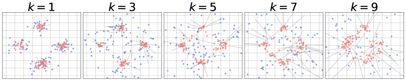
Figure 5: The red particles represent samples drawn from the target distribution, while the blue particles correspond to the noisy data originating from the target distribution. This noise is introduced by corrupting the target distribution with Gaussian noise, characterized by a standard deviation of $k$. The gray lines denote the pairing induced by model.

Appendix F Additional visual results

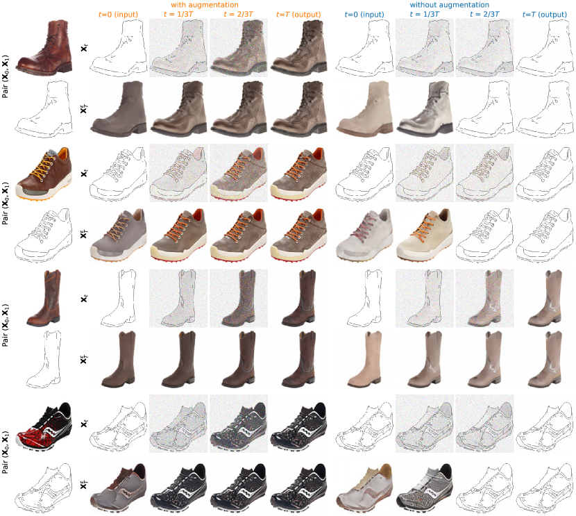
Figure 6: Additional qualitative results between our augmented bridge matching (2nd-5th columns) and standard bridge matching (6th-9th columns) on the bidirectional translation of edges2shoes task.

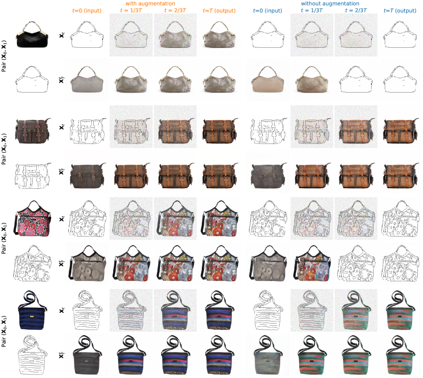
Figure 7: Additional qualitative results between our augmented bridge matching (2nd-5th columns) and standard bridge matching (6th-9th columns) on the bidirectional translation of edges2handbags task.

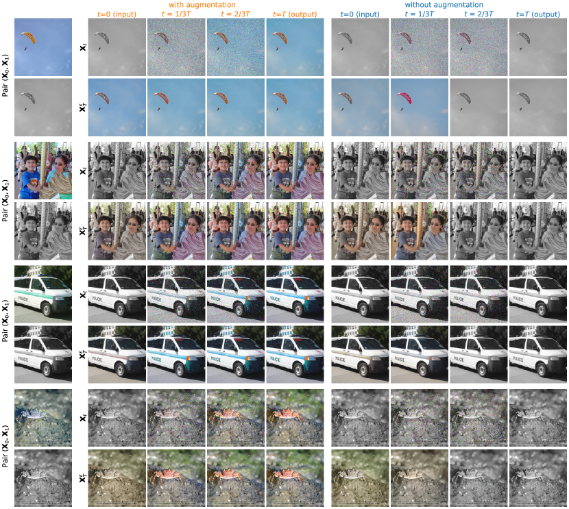
Figure 8: Additional qualitative results between our augmented bridge matching (2nd-5th columns) and standard bridge matching (6th-9th columns) on the bidirectional translation of (de-)colorization task.

References

• Albergo & Vanden-Eijnden (2022) Michael S Albergo and Eric Vanden-Eijnden. Building normalizing flows with stochastic interpolants. arXiv preprint arXiv:2209.15571, 2022.
• Albergo et al. (2023) Michael S Albergo, Nicholas M Boffi, and Eric Vanden-Eijnden. Stochastic interpolants: A unifying framework for flows and diffusions. arXiv preprint arXiv:2303.08797, 2023.
• Barczy & Kern (2013) Mátyás Barczy and Peter Kern. Representations of multidimensional linear process bridges. Random Operators and Stochastic Equations, 21(2):159–189, 2013.
• Chen et al. (2021a) Tianrong Chen, Guan-Horng Liu, and Evangelos A Theodorou. Likelihood training of Schrodinger bridge using forward-backward sdes theory. arXiv preprint arXiv:2110.11291, 2021a.
• Chen et al. (2021b) Yongxin Chen, Tryphon T Georgiou, and Michele Pavon. Optimal transport in systems and control. Annual Review of Control, Robotics, and Autonomous Systems, 4, 2021b.
• Chopin et al. (2023) Nicolas Chopin, Andras Fulop, Jeremy Heng, and Alexandre H Thiery. Computational doob h-transforms for online filtering of discretely observed diffusions. In International Conference on Machine Learning, pp.  5904–5923. PMLR, 2023.
• Chung et al. (2022a) Hyungjin Chung, Byeongsu Sim, Dohoon Ryu, and Jong Chul Ye. Improving diffusion models for inverse problems using manifold constraints. arXiv preprint arXiv:2206.00941, 2022a.
• Chung et al. (2022b) Hyungjin Chung, Byeongsu Sim, and Jong Chul Ye. Come-closer-diffuse-faster: Accelerating conditional diffusion models for inverse problems through stochastic contraction. In Proceedings of the IEEE/CVF Conference on Computer Vision and Pattern Recognition, pp.  12413–12422, 2022b.
• Chung et al. (2023) Hyungjin Chung, Jeongsol Kim, and Jong Chul Ye. Direct diffusion bridge using data consistency for inverse problems. arXiv preprint arXiv:2305.19809, 2023.
• Chung & Walsh (2006) Kai Lai Chung and John B Walsh. Markov processes, Brownian motion, and time symmetry, volume 249. Springer Science & Business Media, 2006.
• Dai Pra (1991) Paolo Dai Pra. A stochastic control approach to reciprocal diffusion processes. Applied mathematics and Optimization, 23(1):313–329, 1991.
• De Bortoli et al. (2021) Valentin De Bortoli, James Thornton, Jeremy Heng, and Arnaud Doucet. Diffusion schrödinger bridge with applications to score-based generative modeling. Advances in Neural Information Processing Systems, 34, 2021.
• Delbracio & Milanfar (2023) Mauricio Delbracio and Peyman Milanfar. Inversion by direct iteration: An alternative to denoising diffusion for image restoration. arXiv preprint arXiv:2303.11435, 2023.
• Dhariwal & Nichol (2021) Prafulla Dhariwal and Alex Nichol. Diffusion models beat GAN on image synthesis. arXiv preprint arXiv:2105.05233, 2021.
• Gyöngy (1986) István Gyöngy. Mimicking the one-dimensional marginal distributions of processes having an itô differential. Probability theory and related fields, 71(4):501–516, 1986.
• Heitz et al. (2023) Eric Heitz, Laurent Belcour, and Thomas Chambon. Iterative $\alpha$-(de) blending: a minimalist deterministic diffusion model. arXiv preprint arXiv:2305.03486, 2023.
• Heng et al. (2021) Jeremy Heng, Valentin De Bortoli, Arnaud Doucet, and James Thornton. Simulating diffusion bridges with score matching. arXiv preprint arXiv:2111.07243, 2021.
• Heusel et al. (2017) Martin Heusel, Hubert Ramsauer, Thomas Unterthiner, Bernhard Nessler, Günter Klambauer, and Sepp Hochreiter. Gans trained by a two time-scale update rule converge to a nash equilibrium. CoRR, abs/1706.08500, 2017. URL http://arxiv.org/abs/1706.08500.
• Ho & Salimans (2022) Jonathan Ho and Tim Salimans. Classifier-free diffusion guidance. arXiv preprint arXiv:2207.12598, 2022.
• Ho et al. (2020) Jonathan Ho, Ajay Jain, and Pieter Abbeel. Denoising diffusion probabilistic models. Advances in Neural Information Processing Systems, 2020.
• Ho et al. (2022) Jonathan Ho, Tim Salimans, Alexey Gritsenko, William Chan, Mohammad Norouzi, and David J Fleet. Video diffusion models. arXiv preprint arXiv:2204.03458, 2022.
• Hyvärinen & Dayan (2005) Aapo Hyvärinen and Peter Dayan. Estimation of non-normalized statistical models by score matching. Journal of Machine Learning Research, 6(4), 2005.
• Isola et al. (2017) Phillip Isola, Jun-Yan Zhu, Tinghui Zhou, and Alexei A Efros. Image-to-image translation with conditional adversarial networks. In Proceedings of the IEEE conference on computer vision and pattern recognition, pp.  1125–1134, 2017.
• Kawar et al. (2022) Bahjat Kawar, Michael Elad, Stefano Ermon, and Jiaming Song. Denoising diffusion restoration models. arXiv preprint arXiv:2201.11793, 2022.
• Léonard (2011) Christian Léonard. Stochastic derivatives and generalized h-transforms of markov processes. arXiv preprint arXiv:1102.3172, 2011.
• Léonard (2012) Christian Léonard. Girsanov theory under a finite entropy condition. In Séminaire de Probabilités XLIV, pp.  429–465. Springer, 2012.
• Léonard (2014) Christian Léonard. A survey of the Schrödinger problem and some of its connections with optimal transport. Discrete & Continuous Dynamical Systems-A, 34(4):1533–1574, 2014.
• Léonard (2022) Christian Léonard. Feynman-kac formula under a finite entropy condition. Probability Theory and Related Fields, 184(3-4):1029–1091, 2022.
• Léonard et al. (2014) Christian Léonard, Sylvie Rœlly, Jean-Claude Zambrini, et al. Reciprocal processes. a measure-theoretical point of view. Probability Surveys, 11:237–269, 2014.
• Lipman et al. (2022) Yaron Lipman, Ricky TQ Chen, Heli Ben-Hamu, Maximilian Nickel, and Matt Le. Flow matching for generative modeling. arXiv preprint arXiv:2210.02747, 2022.
• Liu et al. (2022a) Guan-Horng Liu, Tianrong Chen, Oswin So, and Evangelos A Theodorou. Deep generalized Schrodinger bridge. arXiv preprint arXiv:2209.09893, 2022a.
• Liu et al. (2023) Guan-Horng Liu, Arash Vahdat, De-An Huang, Evangelos A. Theodorou, Weili Nie, and Anima Anandkumar. I2sb: Image-to-image schrödinger bridge, 2023. URL https://arxiv.org/abs/2302.05872.
• Liu (2022) Qiang Liu. Rectified flow: A marginal preserving approach to optimal transport. arXiv preprint arXiv:2209.14577, 2022.
• Liu et al. (2022b) Xingchao Liu, Chengyue Gong, and Qiang Liu. Flow straight and fast: Learning to generate and transfer data with rectified flow. arXiv preprint arXiv:2209.03003, 2022b.
• Liu et al. (2022c) Xingchao Liu, Lemeng Wu, Mao Ye, and Qiang Liu. Let us build bridges: Understanding and extending diffusion generative models. arXiv preprint arXiv:2208.14699, 2022c.
• Lugmayr et al. (2022) Andreas Lugmayr, Martin Danelljan, Andres Romero, Fisher Yu, Radu Timofte, and Luc Van Gool. Repaint: Inpainting using denoising diffusion probabilistic models. In Proceedings of the IEEE/CVF Conference on Computer Vision and Pattern Recognition, pp.  11461–11471, 2022.
• Palmowski & Rolski (2002) Zbigniew Palmowski and Tomasz Rolski. A technique for exponential change of measure for markov processes. Bernoulli, pp.  767–785, 2002.
• Peluchetti (2021) Stefano Peluchetti. Non-denoising forward-time diffusions. 2021.
• Peluchetti (2023) Stefano Peluchetti. Diffusion bridge mixture transports, schrodinger bridge problems and generative modeling. arXiv preprint arXiv:2304.00917, 2023.
• Peyré & Cuturi (2019) Gabriel Peyré and Marco Cuturi. Computational optimal transport. Foundations and Trends® in Machine Learning, 11(5-6):355–607, 2019.
• Pooladian et al. (2023) Aram-Alexandre Pooladian, Heli Ben-Hamu, Carles Domingo-Enrich, Brandon Amos, Yaron Lipman, and Ricky Chen. Multisample flow matching: Straightening flows with minibatch couplings. arXiv preprint arXiv:2304.14772, 2023.
• Poole et al. (2022) Ben Poole, Ajay Jain, Jonathan T Barron, and Ben Mildenhall. Dreamfusion: Text-to-3d using 2d diffusion. arXiv preprint arXiv:2209.14988, 2022.
• Rogers & Williams (2000) L. C. G. Rogers and David Williams. Diffusions, Markov processes, and martingales. Vol. 2. Cambridge Mathematical Library. Cambridge University Press, Cambridge, 2000. ISBN 0-521-77593-0. doi: 10.1017/CBO9781107590120. URL https://doi.org/10.1017/CBO9781107590120. Itô calculus, Reprint of the second (1994) edition.
• Ronneberger et al. (2015) Olaf Ronneberger, Philipp Fischer, and Thomas Brox. U-net: Convolutional networks for biomedical image segmentation. In Medical Image Computing and Computer-Assisted Intervention–MICCAI 2015: 18th International Conference, Munich, Germany, October 5-9, 2015, Proceedings, Part III 18, pp.  234–241. Springer, 2015.
• Saharia et al. (2022a) Chitwan Saharia, William Chan, Huiwen Chang, Chris Lee, Jonathan Ho, Tim Salimans, David Fleet, and Mohammad Norouzi. Palette: Image-to-image diffusion models. In ACM SIGGRAPH 2022 Conference Proceedings, pp.  1–10, 2022a.
• Saharia et al. (2022b) Chitwan Saharia, William Chan, Saurabh Saxena, Lala Li, Jay Whang, Emily Denton, Seyed Kamyar Seyed Ghasemipour, Burcu Karagol Ayan, S Sara Mahdavi, Rapha Gontijo Lopes, et al. Photorealistic text-to-image diffusion models with deep language understanding. arXiv preprint arXiv:2205.11487, 2022b.
• Schrödinger (1932) Erwin Schrödinger. Sur la théorie relativiste de l’électron et l’interprétation de la mécanique quantique. Annales de l’Institut Henri Poincaré, 2(4):269–310, 1932.
• Shi et al. (2022) Yuyang Shi, Valentin De Bortoli, George Deligiannidis, and Arnaud Doucet. Conditional simulation using diffusion schröodinger bridges. arXiv preprint arXiv:2202.13460, 2022.
• Shi et al. (2023) Yuyang Shi, Valentin De Bortoli, Andrew Campbell, and Arnaud Doucet. Diffusion schrodinger bridge matching. arXiv preprint arXiv:2303.16852, 2023.
• Sohl-Dickstein et al. (2015) Jascha Sohl-Dickstein, Eric Weiss, Niru Maheswaranathan, and Surya Ganguli. Deep unsupervised learning using nonequilibrium thermodynamics. In International Conference on Machine Learning, 2015.
• Somnath et al. (2023) Vignesh Ram Somnath, Matteo Pariset, Ya-Ping Hsieh, Maria Rodriguez Martinez, Andreas Krause, and Charlotte Bunne. Aligned diffusion schrödinger bridges, 2023. URL https://arxiv.org/abs/2302.11419.
• Song & Ermon (2019) Yang Song and Stefano Ermon. Generative modeling by estimating gradients of the data distribution. In Advances in Neural Information Processing Systems, 2019.
• Stroock & Varadhan (2007) Daniel W Stroock and SR Srinivasa Varadhan. Multidimensional diffusion processes. Springer, 2007.
• Tamir et al. (2023) Ella Tamir, Martin Trapp, and Arno Solin. Transport with support: Data-conditional diffusion bridges. arXiv preprint arXiv:2301.13636, 2023.
• Thornton et al. (2022) James Thornton, Michael Hutchinson, Emile Mathieu, Valentin De Bortoli, Yee Whye Teh, and Arnaud Doucet. Riemannian diffusion schr$\backslash$” odinger bridge. arXiv preprint arXiv:2207.03024, 2022.
• Tong et al. (2023) Alexander Tong, Nikolay Malkin, Guillaume Huguet, Yanlei Zhang, Jarrid Rector-Brooks, Kilian Fatras, Guy Wolf, and Yoshua Bengio. Conditional flow matching: Simulation-free dynamic optimal transport. arXiv preprint arXiv:2302.00482, 2023.
• Trippe et al. (2022) Brian L Trippe, Jason Yim, Doug Tischer, Tamara Broderick, David Baker, Regina Barzilay, and Tommi Jaakkola. Diffusion probabilistic modeling of protein backbones in 3d for the motif-scaffolding problem. arXiv preprint arXiv:2206.04119, 2022.
• Vargas et al. (2021) Francisco Vargas, Pierre Thodoroff, Neil D. Lawrence, and Austen Lamacraft. Solving schrödinger bridges via maximum likelihood. arXiv preprint arXiv:2106.02081, 2021.
• Vincent (2011) Pascal Vincent. A connection between score matching and denoising autoencoders. Neural Computation, 23(7):1661–1674, 2011.
• Watson et al. (2022) Joseph L Watson, David Juergens, Nathaniel R Bennett, Brian L Trippe, Jason Yim, Helen E Eisenach, Woody Ahern, Andrew J Borst, Robert J Ragotte, Lukas F Milles, et al. Broadly applicable and accurate protein design by integrating structure prediction networks and diffusion generative models. BioRxiv, pp.  2022–12, 2022.
• Zhou et al. (2023) Linqi Zhou, Aaron Lou, Samar Khanna, and Stefano Ermon. Denoising diffusion bridge models. arXiv preprint arXiv:2309.16948, 2023.