CL-Flow:Strengthening the Normalizing Flows by Contrastive Learning for Better Anomaly Detection

Abstract

In the anomaly detection field, the scarcity of anomalous samples has directed the current research emphasis towards unsupervised anomaly detection. While these unsupervised anomaly detection methods offer convenience, they also overlook the crucial prior information embedded within anomalous samples. Moreover, among numerous deep learning methods, supervised methods generally exhibit superior performance compared to unsupervised methods. Considering the reasons mentioned above, we propose a self-supervised anomaly detection approach that combines contrastive learning with 2D-Flow to achieve more precise detection outcomes and expedited inference processes. On one hand, we introduce a novel approach to anomaly synthesis, yielding anomalous samples in accordance with authentic industrial scenarios, alongside their surrogate annotations. On the other hand, having obtained a substantial number of anomalous samples, we enhance the 2D-Flow framework by incorporating contrastive learning, leveraging diverse proxy tasks to fine-tune the network. Our approach enables the network to learn more precise mapping relationships from self-generated labels while retaining the lightweight characteristics of the 2D-Flow. Compared to mainstream unsupervised approaches, our self-supervised method demonstrates superior detection accuracy, fewer additional model parameters, and faster inference speed. Furthermore, the entire training and inference process is end-to-end. Our approach showcases new state-of-the-art results, achieving a performance of 99.6% in image-level AUROC on the MVTecAD dataset and 96.8% in image-level AUROC on the BTAD dataset.

I INTRODUCTION

In the contemporary world, industrial products, ranging from aircraft wings to semiconductor chips, require dependable defect detection to ensure quality. Traditional methods were labor-intensive and inefficient. However, recent advances in computer vision and deep learning have revolutionized industrial defect detection, garnering significant attention in both academia and industry.

In many production processes, due to the scarcity of anomalous samples and the presence of unpredictable anomalous patterns, most of previous anomaly detection methods [5, 22, 32, 40, 15, 30, 39, 36, 37, 33, 19] only modeled normal samples. However, it is worth contemplating whether the absence of anomalous samples and their corresponding labels hinders the model from learning more precise mapping relationships. Recently, some studies[20, 37] have begun incorporating automatically generated negative samples to enhance model performance. But in the work of [20], the incorporation of negative samples was not coupled with more intricate network architectures, and the proxy task configurations were overly simplistic, leading to suboptimal performance. In another study[37], researchers need to manually set classification boundaries to guide training, and the two-stage training process introduces inconvenience. While the aforementioned methods have their limitations, they also open up new avenues for unsupervised anomaly detection. We can explore the direction of self-supervised learning by utilizing automatically generated negative samples, allowing the network to acquire more precise mapping relationships.

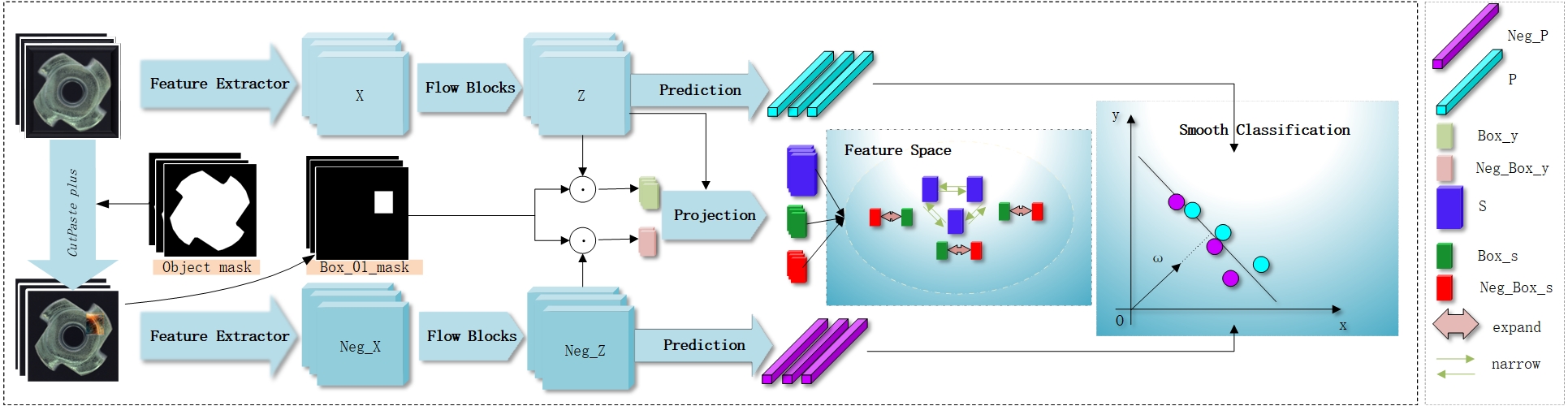
Figure 1: Our model framework is an end-to-end Siamese network, where the upper and lower pathways share the same network weights. In the above figure, we employ Cait as the feature extractor, and the Flow Blocks adopt the 2D-Flow module. The Projection module consists of a simple structure comprising linear, ReLU, and linear layers. The Prediction module is a two-layer linear classifier.

In summary, we introduce CL-Flow shown in Fig.1, a novel self-supervised anomaly detection framework, which leverages 2D-Flow[39] as its baseline and enhances model performance through the integration of contrastive learning. Firstly, we proposed an improved version of the CutPaste method to generate realistic abnormal defects and defect masks. Secondly, both positive and negative samples are fed into the network and projected into a new feature space. Finally, distinct feature distance losses and smooth classification losses are employed in the new feature space to optimize network parameters. The detailed description is in sec III-B.

In addition, we also investigate the widespread applicability of the CL-Flow training approach. Experimental results demonstrate that our method not only enhances the performance of flows models but also shows improvements in the performance of convolutional neural networks[17] and transformers[13, 21]. The detailed description is in sec III-C.

Overall, our main contributions are as follows:

• We introduce a novel self-supervised anomaly detection framework with end-to-end training and inference, achieving elevated detection accuracy while retaining the rapid and lightweight characteristics of the 2D-Flow model.

• We introduce a novel anomaly generation method capable of generating high-quality anomaly samples along with their corresponding region labels. We further incorporate contrastive learning into the 2D-Flow framework to enhance the performance of the base network.

• We have investigated the inherent limitations of pre-trained models trained on ImageNet[10] when applied to anomaly detection datasets, as they may possess prior information that is not applicable. By using novel pretraining methods, we can effectively enhance the adaptability of the feature extractor.

• Our method achieves state-of-the-art image-level and pixel-level accuracy on the MVTecAD [4]dataset and the more challenging BTAD[23] dataset.

II Related work

II-A Unsupervised Anomaly Detection

Existing unsupervised anomaly detection methods can be primarily categorized into reconstruction-based and feature representation-based approaches. Reconstruction-based methods typically employ image generators such as Generative Adversarial Networks (GANs) [14, 31, 41, 32, 2, 25] or teacher-student models [3, 35] to generate or reconstruct input images. These methods also leverage the differences between input images and their reconstructed counterparts to localize the anomalous regions. However, the assumption underlying reconstruction-based methods is not entirely reliable. Even when trained on normal samples only, the model can still fully reconstruct unseen defects and affect detection accuracy.

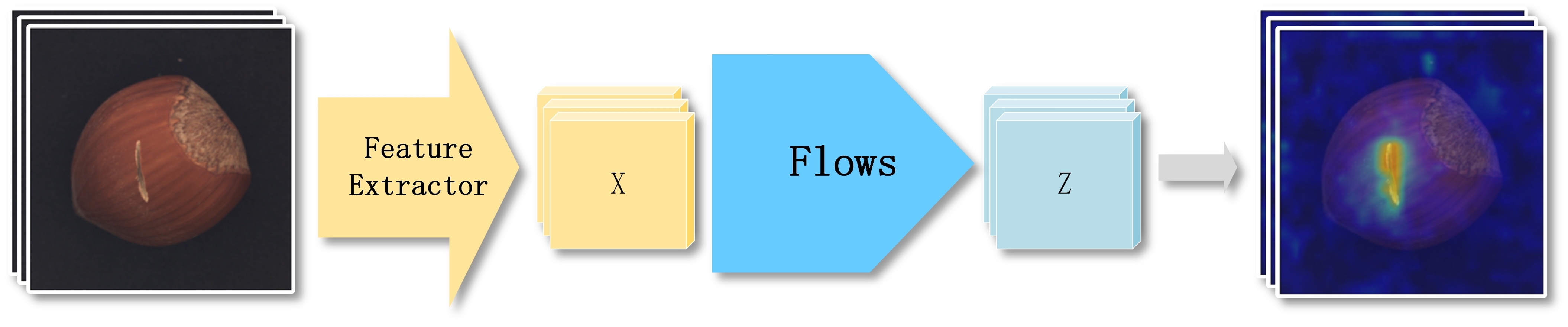
Figure 2: The mainstream framework for anomaly detection utilizing normalizing flows.

Feature representation-based methods typically utilize pre-trained feature extractors to extract image features. One intuitive approach in this category[24, 8, 28] is to construct a positive sample database by using normal images as templates and to localize anomalies by measuring the feature differences between negative samples and the positive sample database. However, this approach has the drawbacks of high storage costs and slow retrieval times. Another approach is to use probabilistic modeling to capture the feature distribution of normal samples, which compares the distributions of normal and anomalous regions without additional storage costs. Rippel et al[27] initially modeled each feature map as a multivariate Gaussian distribution. During testing, the Mahalanobis distance from the feature vector to normal sample distribution detects anomalies. PaDim[9] further extended the modeling of multivariate Gaussian distributions to the granularity of image blocks, enabling pixel-level segmentation. In contrast, DifferNet[29] introduced the concept of normalizing flow (NF) in recent years, providing greater potential for such methods.

II-B Normalizing Flow

Normalizing Flows (NF)[26] transform complex data distributions into simple Gaussian distributions. NF is widely used in generative models and can also perform the inverse transformation. NICE[11], RealNVP[12], and Glow[18] are common NF implementations.

Recent works[29, 15, 30, 39, 37, 19] use pre-trained models to extract features from normal samples and map them to a Gaussian distribution in latent space Z using the NF module. Anomalous samples in Z space exhibit non-Gaussian features with lower likelihood, as shown in Fig.2. DifferNet[29] initially introduced the NF and achieved excellent anomaly classification results at the image level. CFlow-AD[15] achieved initial localization of anomalies at the pixel level. FastFlow[39] introduced the 2D-Flow and accelerated the training and inference process by employing 1x1 convolutions. Although BGAD-FAS[37] initially used self-generated negative samples to optimize classification boundaries during training, the two-stage process and manual boundary delineation posed inconvenience.

II-C Contrastive Learning

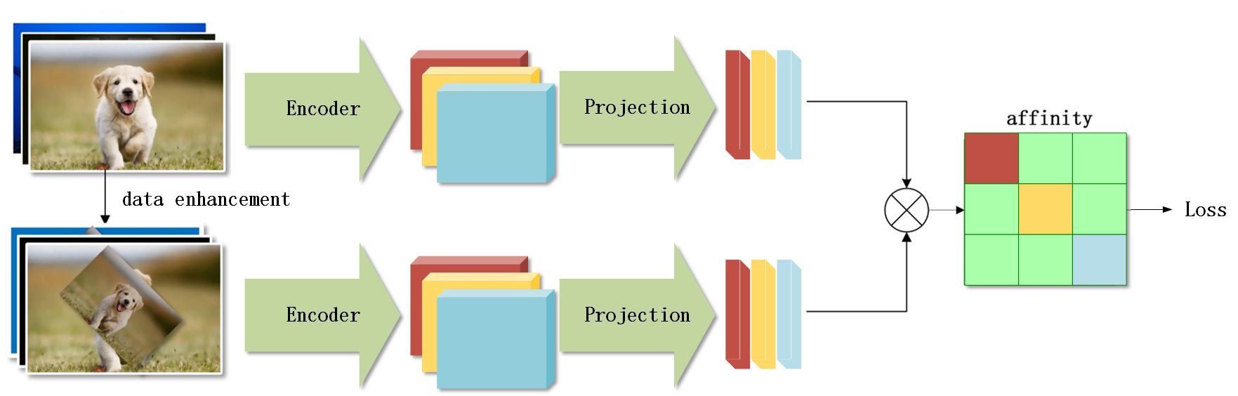
Figure 3: The main process of contrastive learning, which enables the encoder to have excellent feature extraction capabilities.

Contrastive learning is a self-supervised learning method used to enhance the feature extraction capability of networks in the absence of labels. It involves setting up proxy tasks and flexible loss functions to train the network. In recent work, SimCLR[6] and MOCO[16] introduced the concept of automatically generating negative samples and feeding both positive and negative samples into a Siamese network. By maximizing the feature similarity between positive sample pairs within a training batch and minimizing the feature similarity between positive and negative sample pairs, the network learns the features of the dataset, as shown in Fig.3.

Our approach combines contrastive learning with the normalizing flow, introducing a novel self-supervised anomaly detection framework.

III Method

III-A CutPaste Plus

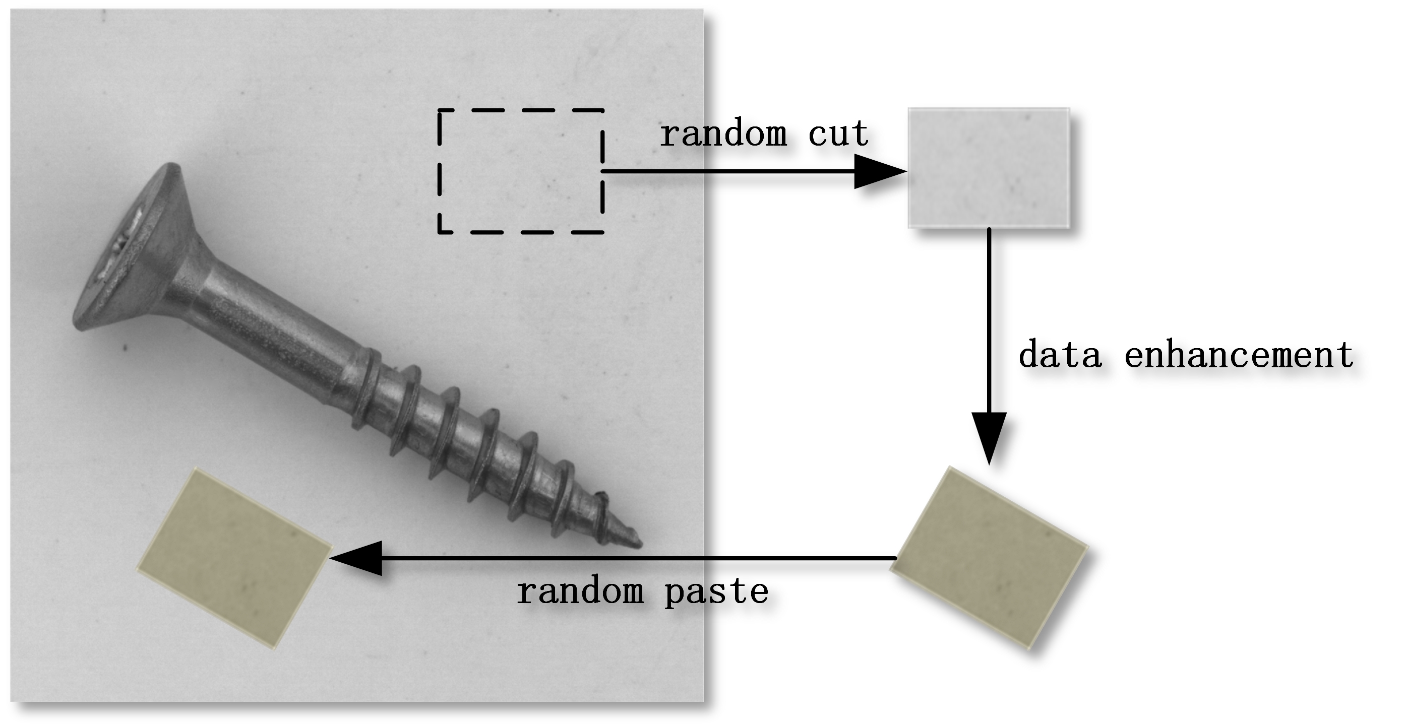
Figure 4: The initial CutPaste method generates substandard abnormal images, which undermine the performance of the model.

In self-supervised methods that require negative samples, the quality of negative samples is especially crucial. It is essential to emphasize that low-quality negative samples not only fail to augment the model’s expressive capabilities but may also inflict substantial detriment to its overall performance.

CutPaste[20] is a data augmentatio technique that involves randomly cropping patches from the original image and pasting them back into random locations within the same image to create anomaly images. While this method can generate high-quality anomalies in texture datasets, it presents challenges in object datasets. As illustrated in Fig.4, these patches are pasted onto the background of the screw images. But in anomaly detection tasks, we often need to disregard the background. Consequently, negative samples produced by this approach are of poor quality and have limited practicality in real-world scenarios.

In summary, we have made improvements to the CutPaste method. Specifically, we incorporate the FT[1] saliency detection algorithm to generate object masks for images before training. The FT saliency detection algorithm is a frequency-tuned approach that analyzes an image’s energy distribution at various frequencies in order to identify regions of interest. For randomly cropped patches from the original image, we used the object mask to confine their pasting area, ensuring that they solely introduce defects into the foreground of the image. Additionally, we recorded the defect locations as anomaly region labels, which facilitated subsequent processing of local features in samples. As shown in Table V, CutPaste Plus significantly enhances anomaly detection across most object-class datasets.

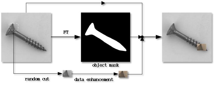
Figure 5: The CutPaste Plus method restricts the pasting area of abnormal patches and records it to generate authentic and effective anomaly samples.

III-B CL-Flow

In mathematical notation, we represent our normalization flow as $f_{\theta}:\mathcal{X}\in\mathbb{R}^{d}\rightarrow\mathcal{Z}\in\mathbb{R}^{d}$ , where $\mathcal{X}\in\mathbb{R}^{d}$ denotes the original feature space, $\mathcal{Z}\in\mathbb{R}^{d}$ denotes the transformed space and $d$ denotes the feature dimensions. In recent studies, the principle of utilizing normalization flows for anomaly detection can be summarized as follows. The normal samples are first passed through a feature extractor, which can be either a VIT or a CNN. The resulting feature maps $x$ are then transformed using the NF into latent tensors $z$ that follow a Gaussian distribution, as shown in the equation:

$$p_{X}(x)=p_{Z}(z)\left|\operatorname{det}\left(\frac{\partial z}{\partial x}\right)\right|$$ (1)

We optimize this transformation process by maximizing the log-likelihood:

$$\log p_{X}(x) =\log p_{Z}(z)+\log\left|\operatorname{det}\left(\frac{\partial z}{\partial x}\right)\right|$$ (2)

$$=\log p_{Z}\left(f_{\theta}(x)\right)+\log\left|\operatorname{det}\left(\frac{\partial f_{\theta}(x)}{\partial x}\right)\right|$$

Here, $\operatorname{det}\left(\frac{\partial f_{\theta}(x)}{\partial x}\right)$ represents the Jacobian matrix of the invertible transformations ${z}=f_{\theta}(x)$ and ${x}=f_{\theta}^{-1}(z)$, and $\theta$ represents the parameters of the flow model. We typically assume $z\sim\mathcal{N}(0,I)$ :

$$p_{Z}(z)=(2\pi)^{-\frac{d}{2}}\mathrm{e}^{-\frac{1}{2}z^{T}z}$$ (3)

Substituting it into equation (2), we have:

$$\log p_{X}(x)=-\left[\frac{1}{2}f_{\theta}(x)^{T}f_{\theta}(x)-\log\left|\operatorname{det}\left(\frac{\partial z}{\partial x}\right)\right|+\frac{d}{2}\log(2\pi)\right]$$ (4)

The NF loss function can be defined as:

$$\mathcal{L}_{ml}=\frac{1}{2}f_{\theta}(x)^{T}f_{\theta}(x)-\log\left|\operatorname{det}\left(\frac{\partial z}{\partial x}\right)\right|+\frac{d}{2}\log(2\pi)$$ (5)

In CL-Flow, we continue to use the strategy of NF, but we introduce negative samples to construct a Siamese network and add new loss functions to strengthen the network, as shown in Fig.1. During the training phase, the negative samples generated through the CutPaste Plus method are introduced into the network along with the positive samples. Additionally, our CutPaste Plus module records the abnormal region Box_01_mask. The resulting Z and Neg_Z from the Flow Blocks module are multiplied by Box_01_mask, yielding Box_y and Neg_Box_y respectively. Subsequently, Box_y and Neg_Box_y, along with Z, are input into the Projection module to obtain Box_s, Neg_Box_s and S. We optimize the network parameters by minimizing the feature distance between the S tensors while expanding the feature distance between Box_s and Neg_Box_s using (6):

$$\mathcal{L}_{pnd}= -\log\left\{\sum_{\mathrm{i}=1}^{\mathrm{K}}\sum_{\mathrm{j}=1}^{\mathrm{K}}1_{[\mathrm{i}\neq\mathrm{j}]}\mathrm{F}\left(\mathrm{S}_{\mathrm{i}},\mathrm{S}_{\mathrm{j}}\right)+\right.$$ (6)

$$\left.\sum_{\mathrm{i}=1}^{\mathrm{K}}\left[1-\mathrm{F}\left(\text{ Box\_s}_{\mathrm{i}},\text{ Neg\_Box\_s}_{\mathrm{i}}\right)\right]\right\}$$

In (6), $\mathrm{K}$ represents the batch size, $\mathrm{F}$ denotes the cosine similarity function, $\mathrm{S}$ represents the features of positive samples, $\mathrm{Neg\_Box\_s}$ represents the features of anomalous regions in negative samples and $\mathrm{Box\_s}$ represents the features of corresponding regions in positive samples.

Apart from that, Z and Neg_Z are separately processed through the Prediction module to obtain P and Neg_P, and further network parameter optimization is achieved using (7):

$$\mathcal{L}_{scf}=\text{CELoss }^{\tau}\left(\mathrm{Neg}\_{\mathrm{P}},1\right)+\text{ CELoss }{}^{\tau}(\mathrm{P},0)$$ (7)

where $\mathrm{CELoss}$ represents $\mathrm{CrossEntropyLoss}$, and $\tau$ is the label smoothing coefficient. Table IV have shown that if label smoothing is not applied, $\mathcal{L}_{scf}$ can negatively impact the model’s performance. This is because the object category of anomalous samples is fundamentally the same as that of normal samples, and our goal is to determine whether they contain defects.

Finally, the overall loss of CL-Flow can be defined as follows:

$$\mathcal{L}=\mathcal{L}_{ml}+\lambda_{1}\mathcal{L}_{pnd}+\lambda_{2}\mathcal{L}_{scf}$$ (8)

During the inference stage, only $\mathcal{L}_{ml}$ is retained for anomaly assessment. The settings of $\lambda_{1}$ and $\lambda_{2}$ need to ensure that all three loss functions remain on the same scale of magnitude at the beginning of training.

TABLE I: Complexity Analysis of Anomaly Detection Methods based on Flow.

	FPS				Additional Params
backbone	CFlow	FastFlow	U-Flow	CL-Flow(ours)	CFlow	FastFlow	U-Flow	CL-Flow(ours)
ResNet18	40.5	61.3	32.7	65.2	5.5M	4.9M	4.3M	4.5M
WideResnet50-2	24.3	40.6	21.4	42.1	81.6M	41.3M	34.8M	36.2M
DeiT-base-distilled	30.0	52.1	-	56.3	10.5M	14.8M	-	10.2M
CaiT-M48-distilled	5.5	8.1	-	8.5	10.5M	14.8M	-	10.2M
MS-CaIT	-	-	3.3	-	-	-	12.2M	-

III-C Feature Extractor

In previous works, the feature extractors were typically pretrained on the ImageNet[10] dataset, which may not be applicable to anomaly detection datasets. Therefore, we investigated novel pretraining approaches on the DeiT[34] and ResNet[17] models, encompassing transfer learning, traditional contrastive learning, as well as our CL-Flow method illustrated in Fig.1.

For transfer learning, we appended a classification head to the feature extractor and trained it on the normal samples of the MVTec AD[4] dataset for a 15-class classification task. And for contrastive learning, we employed SimSiam[7] for transfer learning on the backbone network, which is a traditional contrastive learning method proposed in 2021 and has outperformed contemporary contrastive learning models.

Furthermore, we employed the CL-Flow approach to train individual feature extractors for each specific class dataset. Specifically, we utilized CutPaste Plus to generate negative samples. For the positive and negative samples’ features obtained from the backbone output, we applied cosine similarity loss on the anomaly box regions and used label smoothing for the final binary classification task. The experimental results are presented in Table IV.

TABLE II: We present the results in the format (image-level, pixel-level) of our method and other state-of-the-art approaches in anomaly detection and localization on the MVTec AD dataset.

Category	Draem[2021]	Padim[2021]	Patch-Core[2022]	CFlow[2021]	CSFlow[2022]	FastFlow[2021]	PyramidFlow[2023]	CL-Flow(ours)[2023]
Carpet	(97.0,95.5)	(-,99.1)	(98.7,98.9)	(100.0,99.3)	(99.0,-)	(100.0,99.4)	( - ,97.4)	(100.0,99.4)
Grid	(99.9,99.7)	(-,97.3)	(98.2,98.7)	(97.6,99.0)	(100.0,-)	(99.7,98.3)	( - ,95.7)	(100.0,98.7)
Leather	(100.0,98.6)	(-,99.2)	(100.0,99.3)	(97.7,99.7)	(100.0,-)	(100.0,99.5)	( - ,98.7)	(100.0,99.6)
Tile	(99.6,99.2)	(-,94.1)	(98.7,95.6)	(98.7,98.0)	(100.0,-)	(100.0,96.3)	( - ,97.1)	(100.0,96.9)
Wood	(99.1,96.4)	(-,94.9)	(99.2,95.0)	(99.6,96.7)	(100.0,-)	(100.0,97.0)	( - ,97.0)	(100.0,96.8)
Av. texture	(99.1,97.8)	(-,96.9)	(98.9,95.7)	(98.7,98.5)	(99.8,-)	(99.9,98.1)	( - ,97.1)	(100.0,98.3)
Bottle	(99.2,99.1)	(-,98.3)	(100.0,98.6)	(100.0,99.0)	(99.8,-)	(100.0,97.7)	( - ,97.8)	(100.0,98.3)
Cable	(91.8,94.7)	(-,96.7)	(99.5,98.4)	(100.0,97.6)	(99.1,-)	(100.0,98.4)	( - ,91.8)	(99.0,98.5)
Capsule	(98.5,94.3)	(- ,98.5)	(98.1,98.8)	(99.3 ,99.0)	(97.1,-)	(100.0,99.1)	( - ,98.6)	(98.8,99.1)
Hazelnut	(100.0,99.7)	(- ,98.2)	(100.0,98.7)	(96.8 ,98.9)	(99.6,-)	(100.0,99.1)	( - ,98.1)	(99.8,99.3)
Metal nut	(98.7,99.5)	(-,97.2)	(100.0,98.4)	(91.9,98.6)	(99.1,-)	(100.0,98.5)	( - ,97.2)	(100.0,98.3)
Pill	(98.9,97.6)	(-,95.7)	(96.6,97.1)	(99.9,99.0)	(98.6,-)	(99.4,99.2)	( - ,94.2)	(98.9,99.1)
Screw	(93.9,97.6)	(-,98.5)	(98.1,99.4)	(99.7,98.9)	(97.6,-)	(97.8,99.4)	( - ,94.6)	(98.3,99.5)
Toothbrush	(100.0,98.1)	(-,98.8)	(100.0,98.7)	(95.2,99.0)	(91.9,-)	(94.4 ,98.9)	( - ,98.5)	(100.0,99.2)
Transistor	(93.1,90.9)	(-,97.5)	(100.0,96.3)	(99.1 ,98.0)	(99.3,-)	(99.8,97.3)	( - ,96.9)	(100.0,97.0)
Zipper	(100.0,98.8)	(-,98.5)	(98.8,98.8)	(98.5 ,99.1)	(99.7,-)	(99.5,98.7)	( - ,96.6)	(100.0,98.7)
Av. objects	(97.1,97.0)	(-,97.7)	(99.1,99.3)	(98.0,98.6)	(98.2,-)	(99.1,98.7)	( - ,97.0)	(99.5,98.7)
Av. total	(98.0,97.3)	(97.9,97.5)	(99.1,98.1)	(98.3,98.6)	(98.7,-)	(99.4,98.5)	( - ,97.1)	(99.6,98.6)

IV Experiments

IV-A Datasets and Metrics

We evaluated our method on the MVTec Anomaly Detection Dataset[4] (MVTecAD) and BeanTech Anomaly Detection Dataset[23] (BTAD). MVTec AD contains high-resolution images from 15 categories with both normal and anomalous samples. The training set only includes normal samples, while the test set contains both. BTAD dataset consists of texture images captured in real industrial scenes, featuring three different categories. The defects present in each category are subtle and difficult to distinguish with the naked eye, posing greater challenges for anomaly classification and localization.

We employed AUROC (Area Under the Receiver Operating Characteristic curve) as the evaluation metric for our experiments. It is widely used in anomaly detection to compare and assess the performance of different models or algorithms. It measures the performance of a classifier by plotting the true positive rate against the false positive rate at various classification thresholds. The AUROC score represents the area under this curve, which ranges from 0 to 1.

TABLE III: Quantitative results in the format (image-level, pixel-level) of CL-Flow and other outstanding methods approaches in anomaly detection and localization on the BTAD dataset.

Methods	Classes			Mean
	01	02	03
VT-ADL[2021]	(97.6,99.0)	(71.0,94.0)	(82.6,77.0)	(83.7,90.0)
P-SVDD[2020]	(95.7,91.6)	(72.1,93.6)	(82.1,91.0)	(83.3,92.1)
SPADE[2020]	(91.4,97.3)	(71.4,94.4)	(99.9,99.1)	(87.6,96.9)
PaDiM[2021]	(99.8,97.0)	(82.0,96.0)	(99.4,98.8)	(93.7,97.3)
PatchCore[2022]	(90.9,95.5)	(79.3,94.7)	(99.8,99.3)	(90.0,96.5)
FastFlow[2021]	(-,95.0)	(-,96.0)	(-,99.0)	(-,96.6)
PyramidFlow[2023]	(100.0,97.4)	(88.2,97.6)	(99.3,98.1)	(95.8,97.7)
CL-Flow(ours)[2023]	(100.0,99.0)	(91.1,95.8)	(99.4,99.3)	(96.8,98.0)

TABLE IV: Anomaly detection and localization results in the format (image-level, pixel-level) on the MVTecAD dataset based on CutPaste Plus. 2D-Flow means the baseline network.

	w/o Abnormal Samples	w/ Abnormal Samples
Object Category	2D-Flow	CutPaste	CutPaste Plus
Bottle	(100.0,97.7)	(100.0,97.6)	(100.0,98.3)
Cable	(98.5,98.3)	(96.5,98.2)	(99.0,98.5)
Capsule	(98.3,99)	(98.5,98.8)	(98.8,99.1)
Hazelnut	(99.9,99.1)	(98.3,99.2)	(99.8,99.3)
Metal nut	(100.0,98.5)	(100.0,97.6)	(100.0,98.3)
Pill	(97.6,98.8)	(98.3,99.0)	(98.9,99.1)
Screw	(94.8,99.4)	(93.9,99.4)	(98.3,99.5)
Toothbrush	(94.9,98.9)	(91.6,99.0)	(100.0,99.2)
Transistor	(99.7,96.6)	(97.4,98.3)	(100.0,97.0)
Zipper	(99.5,98.6)	(100.0,98.8)	(100.0,98.7)
Mean	(98.3,98.4)	(97.4,98.5)	(99.5,98.7)

IV-B Complexity Analysis

We evaluated the computational complexity of CL-Flow and other Flow methods in terms of FPS and additional model parameters (excluding the backbone network parameters). The hardware configuration of the machine used for testing is Intel(R) Xeon(R) Silver 4310 CPU @ 2.10GHz and NVIDIA Geforce RTX 3090 GPU (24GB graphics memory). The backbone used in our study were VIT (CaiT and DeiT) and ResNet. Compared to CFlow, CL-Flow achieves faster inference speed and smaller model parameters due to the utilization of lightweight 2D-Flow modules. In comparison to FastFlow, CL-Flow utilizes fewer (16 blocks for VIT) Flow blocks. When compared to U-Flow, CL-Flow does not require multiple backbone networks applied at different scales, resulting in faster inference speed. The comparison results are shown in Table I.

TABLE V: Detailed investigation experiments on the CL-Flow architecture, including the use of negative samples, the inclusion of projection, and the determination of smoothing coefficient for classification task.

Category	w/o AS	w/ AS
	$\mathcal{L}_{ml}$	$\mathcal{L}_{ml}+\mathcal{L}_{pnd}$		$\mathcal{L}_{ml}+\mathcal{L}_{scf}$				$\mathcal{L}_{ml}+\mathcal{L}_{pnd}+\mathcal{L}_{scf}$
		w/o projection	A.w/ projection	$\tau$=0	$\tau$=0.2	B.$\tau$=0.35	$\tau$=0.5	A+B
Carpet	(99.9,98.6)	(99.6,98.9)	(100.0,99.1)	(99.9.98.6)	(98.9,99.2)	(100.0,99.3)	(98.9,99.1)	(100.0,99.4)
Grid	(100.0,95.2)	(99.1,97.1)	(99.9,97.4)	(100.0,95.2)	(100.0,98.0)	(100.0,98.2)	(100.0,97.6)	(100.0,98.7)
Leather	(100.0,99.3)	(100.0,99.5)	(100.0,99.5)	(100.0,99.3)	(100.0,99.3)	(100.0,99.3)	(100.0,99.3)	(100.0,99.6)
Tile	(99.9,94.4)	(100.0,95.3)	(100.0,96.7)	(99.9,94.4)	(100.0,95.4)	(100.0,96.3)	(100.0,95.4)	(100.0,96.9)
Wood	(98.4,93.6)	(99.4,95.0)	(99.6,96.3)	(98.4,93.6)	(99.5,93.4)	(100.0,96.8)	(99.7,93.0)	(100.0,96.8)
Bottle	(100.0,97.7)	(100.0,97.8)	(100.0,98.1)	(99.8,96.4)	(99.9,98.1)	(100.0,98.3)	(100.0,98.0)	(100.0,98.3)
Cable	(98.5,98.3)	(98.5,98.0)	(99.3,98.4)	(88.7,97.3)	(96.4,97.8)	(98.4,98.4)	(97.6,98.2)	(99.0,98.5)
Capsule	(98.3,99)	(93.0,98.6)	(98.0,99.1)	(93.8,97.9)	(98.3,98.9)	(98.5,99.0)	(97.8,98.8)	(98.8,99.1)
Hazelnut	(99.9,99.1)	(98.0,98.3)	(99.7,99.4)	(95.7,97.5)	(98.5,99.2)	(99.5,99.2)	(96.8,99.2)	(99.8,99.3)
Metal nut	(100.0,98.5)	(100.0,97.7)	(100.0,98.1)	(100.0,95.5)	(100.0,98.0)	(100.0,98.3)	(100.0,97.8)	(100.0,98.3)
Pill	(97.6,98.8)	(95.5,97.8)	(98.9,99.1)	(92.8,96.8)	(98.9,98.7)	(98.7,99.2)	(98.3,98.5)	(98.9,99.1)
Screw	(94.8,99.4)	(78.7,95.0)	(98.0,99.4)	(89.6,97.3)	(95.1,99.4)	(96.7,99.2)	(89.3,99.2)	(98.3,99.5)
Toothbrush	(94.9,98.9)	(99.4,99.1)	(99.4,99.3)	(100.0,98.3)	(96.1,98.9)	(100.0,99.1)	(90.8,99.1)	(100.0,99.2)
Transistor	(99.7,96.6)	(97.9,93.1)	(99.8,97.0)	(97.2,93.4)	(99.0,95.9)	(99.5,96.6)	(99.1,96.0)	(100.0,97.0)
Zipper	(99.5,98.6)	(99.3,98.2)	(99.6,98.5)	(100.0,98.6)	(99.9,98.6)	(100.0,98.7)	(99.8,98.7)	(100.0,98.7)
Av. total	(98.7,97.6)	(97.2,97.2)	(99.5,98.4)	(97.0,96.7)	(98.7,97.9)	(99.4,98.3)	(97.9,97.9)	(99.6,98.6)

IV-C Comparison with state-of-art methods

IV-C1 MVTecAD

We compared CF-Flow with other state-of-the-art anomaly detection methods, including reconstruction-based (Draem[40]), feature distance-based (Padim[9], PatchCore[28]), and most of the Flow-based (CFlow[15], CSFlow[30], FastFlow[39]) approaches under the metrics of image-level AUC and pixel-level AUC. Detailed comparison results for all categories can be found in Table II. Among them, CL-Flow surpasses all other methods by achieving an Image-AUROC of 99.6% and a Pixel-AUROC of 98.6%.

IV-C2 BTAD

We conducted a comparative analysis of various anomaly detection and localization methods, namely VT-ADL[23], P-SVDD[38], SPADE[8], PatchCore[28], PaDiM[9], FastFlow[39], and PyramidFlow[19] on the BTAD dataset. The corresponding results have been presented in Table III. Among all the algorithms, CL-Flow demonstrated superior performance with a image-level AUROC of 96.8% and a pixel-level AUROC of 98.0%.

IV-D Ablation Study

We initially assessed CutPaste Plus against the original CutPaste on object-class datasets, as shown in Table IV. Training with the architecture in Fig.1, experiments indicate that inappropriate anomaly generation methods, such as CutPaste, can harm model performance.

Subsequently, we conducted ablation experiments on the architecture of CL-Flow. In TableV, w/o AS represents the baseline network without using negative samples, and $\mathcal{L}_{ml}$ refers to the loss function of the baseline network in (8). A denotes the incorporation of negative samples into $\mathcal{L}_{pnd}$ calculation, which requires feature projection onto a distinct feature space. B represents the optimal performance achieved by adding the $\mathcal{L}_{scf}$ (7) on the baseline, with a label smoothing coefficient of 0.35.

IV-E Feature extractor and new transfer learning method

We investigated the impact of different pretraining methods on anomaly detection performance using various feature extractors, including wide_resnet50_2[17] and Deit[34], within the testing framework of 2D-Flow. Different pretraining methods have been explained in sec III-C. In TableVI, a represents pre-training using the ImageNet dataset, b represents transfer learning on a 15-class classification task, c represents transfer learning using the SimSiam framework , and d represents a new transfer learning method under the CL-Flow architecture. The new transfer learning method demonstrated the best performance in terms of image-level AUROC, further validating the effectiveness and comprehensiveness of the CL-Flow training approach.

TABLE VI: Results in the format (image-level, pixel-level) of anomaly detection and localization using different pre-training methods on the feature extractors.

	Deit				wide_resnet50_2
Category	a	b	c	d(ours)	a	b	c	d(ours)
Carpet	(100.0,99.3)	(100.0,99.0)	(100.0,99.0)	(100.0,99.3)	(99.3,98.6)	(97.8,97.5)	(98.0,97.6)	(99.9,98.3)
Grid	(98.5,98.0)	(98.1,97.7)	(98.5,98.0)	(100.0,98.4)	(100.0,99.2)	(100.0,99.1)	(100.0,98.9)	(100.0,99.3)
Leather	(100.0,99.4)	(100.0,99.3)	(100.0,99.3)	(100.0,99.3)	(100.0,99.5)	(100.0,98.7)	(100.0,98.5)	(100.0,99.6)
Tile	(100.0,96.3)	(100.0,96.4)	(100.0,92.7)	(100.0,96.4)	(100.0,96.4)	(100.0,97.4)	(100.0,97.2)	(100.0,97.5)
Wood	(97.2,96.1)	(99.4,97.2)	(99.4,96.5)	(100.0,96.4)	(99.4,95.6)	(98.4,95.6)	(99.1,96.2)	(100.0,96.7)
Bottle	(98.4,98.1)	(99.6,97.8)	(99.5,97.9)	(100.0,98.0)	(100.0,98.5)	(100.0,98.4)	(99.5,96.8)	(100.0,98.8)
Cable	(97.9,97.8)	(98.2,97.5)	(99.1,96.9)	(100.0,98.1)	(98.2,97.0)	(97.1,96.9)	(99.7,95.1)	(100.0,96.9)
Capsule	(97.4,98.4)	(98.9,98.8)	(98.1,98.4)	(99.0,98.5)	(98.2,98.8)	(98.5,99.0)	(98.2,98.6)	(99.1,99.0)
Hazelnut	(98.4,99.1)	(99.5,99.2)	(99.6,98.8)	(99.6,99.0)	(99.5,98.3)	(98.2,97.8)	(98.5,97.9)	(99.3,98.1)
Metal nut	(99.7,97.5)	(99.1,94.6)	(98.6,95.7)	(100.0,97.3)	(99.9,99.4)	(99.9,98.5)	(99.7,98.8)	(100.0,99.0)
Pill	(97.4,98.8)	(91.2,98.5)	(95.1,97.9)	(98.2,98.5)	(98.8,97.6)	(97.0,97.6)	(97.6,97.0)	(99.2,98.3)
Screw	(94.1,99.1)	(89.6,99.2)	(86.3,98.3)	(97.4,98.9)	(90.6,98.0)	(88.5,97.4)	(89.9,98.4)	(95.3,99.2)
Toothbrush	(93.3,98.6)	(92.2,98.4)	(93.0,98.1)	(95.1,98.5)	(95.5,98.4)	(93.0,97.8)	(93.6,97.8)	(98.8,98.6)
Transistor	(99.5,93.9)	(99.9,97.0)	(99.2,95.3)	(100.0,95.6)	(99.6,97.6)	(97.0,98.3)	(97.3,97.9)	(100.0,97.5)
Zipper	(99.4,98.3)	(98.1,97.8)	(98.9,98.1)	(99.4,98.0)	(99.5,98.6)	(98.2,98.0)	(99.2,98.5)	(100.0,98.9)
Av. total	(98.1,97.9)	(97.6,97.9)	(97.7,97.4)	(99.2,98.0)	(98.6,98.1)	(97.6,97.9)	(98.0,97.6)	(99.4,98.3)

IV-F Qualitative Results

During the inference stage, we utilize Matplotlib to construct output feature distribution maps as shown in Fig.6. While CL-Flow does not directly modify the structure of the 2D-Flow module, the employed proxy tasks indirectly optimize the performance of the 2D-Flow module.

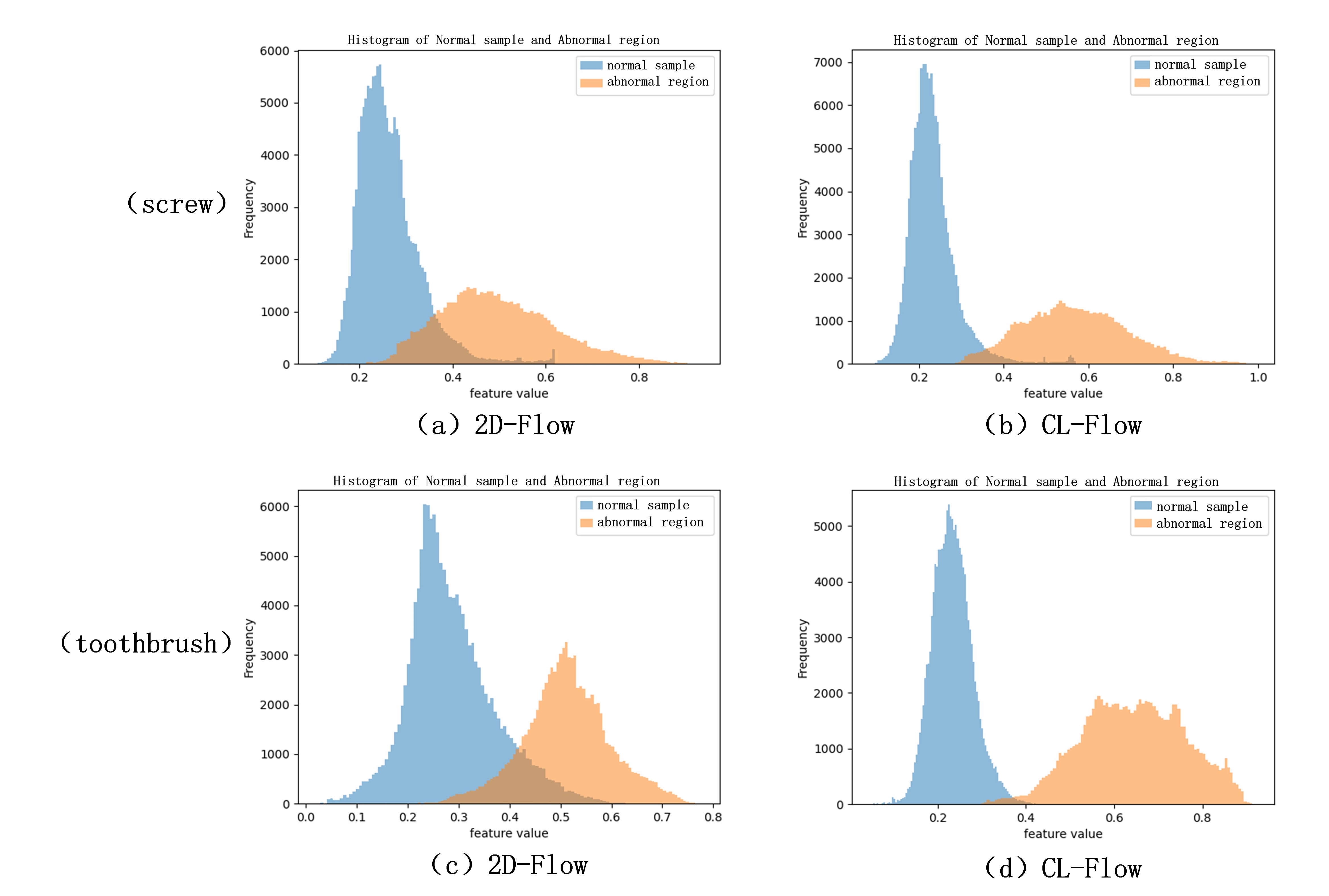
Figure 6: Feature distribution plots of the output features from the Flow Blocks.

V CONCLUSION

In this paper, we introduce CL-Flow, an efficient self-supervised algorithm for anomaly detection and localization. Our end-to-end approach balances high detection accuracy with the Flow model’s speed and lightweight nature. We propose CutPaste Plus for generating realistic negative samples and incorporate contrastive learning into 2D-Flow to optimize model parameters. CL-Flow achieves state-of-the-art image-level and pixel-level accuracy on MVTecAD and BTAD datasets. However, there is potential for improvement, particularly in pixel-level anomaly localization due to the lack of a mainstream multi-scale fusion module. Future work will address this limitation by focusing on fine-grained image feature handling. In summary, CL-Flow presents a promising solution for anomaly detection and localization.

References

- [1] Radhakrishna Achanta, Sheila Hemami, Francisco Estrada, and Sabine Susstrunk. Frequency-tuned salient region detection. In 2009 IEEE conference on computer vision and pattern recognition, pages 1597–1604. IEEE, 2009.
- [2] Samet Akçay, Amir Atapour-Abarghouei, and Toby P Breckon. Skip-ganomaly: Skip connected and adversarially trained encoder-decoder anomaly detection. In 2019 International Joint Conference on Neural Networks (IJCNN), pages 1–8. IEEE, 2019.
- [3] Paul Bergmann, Michael Fauser, David Sattlegger, and Carsten Steger. Uninformed students: Student-teacher anomaly detection with discriminative latent embeddings. In Proceedings of the IEEE/CVF conference on computer vision and pattern recognition, pages 4183–4192, 2020.
- [4] Paul Bergmann., Michael Fauser., and David Sattlegger.and Carsten Steger. Mvtec ad–a comprehensive real-world dataset for unsupervised anomaly detection. In Proceedings of the IEEE/CVF conference on computer vision and pattern recognition, page 9592–9600.
- [5] Paul Bergmann, Sindy Löwe, Michael Fauser, David Sattlegger, and Carsten Steger. Improving unsupervised defect segmentation by applying structural similarity to autoencoders. In VISIGRAPP (5: VISAPP), 2018.
- [6] Ting Chen, Simon Kornblith, Mohammad Norouzi, and Geoffrey Hinton. A simple framework for contrastive learning of visual representations. In International conference on machine learning, pages 1597–1607. PMLR, 2020.
- [7] Xinlei Chen and Kaiming He. Exploring simple siamese representation learning. In Proceedings of the IEEE/CVF conference on computer vision and pattern recognition, pages 15750–15758, 2021.
- [8] Niv Cohen and Yedid Hoshen. Sub-image anomaly detection with deep pyramid correspondences. arXiv preprint arXiv:2005.02357, 2020.
- [9] Thomas Defard, Aleksandr Setkov, Angelique Loesch, and Romaric Audigier. Padim: a patch distribution modeling framework for anomaly detection and localization. In International Conference on Pattern Recognition, pages 475–489. Springer, 2021.
- [10] Jia Deng, Wei Dong, Richard Socher, Li-Jia Li, Kai Li, and Li Fei-Fei. Imagenet: A large-scale hierarchical image database. In 2009 IEEE conference on computer vision and pattern recognition, pages 248–255. Ieee, 2009.
- [11] Laurent Dinh, David Krueger, and Yoshua Bengio. Nice: Non-linear independent components estimation. arXiv preprint arXiv:1410.8516, 2014.
- [12] Laurent Dinh, Jascha Sohl-Dickstein, and Samy Bengio. Density estimation using real nvp. arXiv preprint arXiv:1605.08803, 2016.
- [13] Alexey Dosovitskiy, Lucas Beyer, Alexander Kolesnikov, Dirk Weissenborn, Xiaohua Zhai, Thomas Unterthiner, Mostafa Dehghani, Matthias Minderer, Georg Heigold, Sylvain Gelly, et al. An image is worth 16x16 words: Transformers for image recognition at scale. arXiv preprint arXiv:2010.11929, 2020.
- [14] Ian Goodfellow, Jean Pouget-Abadie, Mehdi Mirza, Bing Xu, David Warde-Farley, Sherjil Ozair, Aaron Courville, and Yoshua Bengio. Generative adversarial networks. Communications of the ACM, 63(11):139–144, 2020.
- [15] Denis Gudovskiy, Shun Ishizaka, and Kazuki Kozuka. Cflow-ad: Real-time unsupervised anomaly detection with localization via conditional normalizing flows. In Proceedings of the IEEE/CVF Winter Conference on Applications of Computer Vision, pages 98–107, 2022.
- [16] Kaiming He, Haoqi Fan, Yuxin Wu, Saining Xie, and Ross Girshick. Momentum contrast for unsupervised visual representation learning. In Proceedings of the IEEE/CVF conference on computer vision and pattern recognition, pages 9729–9738, 2020.
- [17] Kaiming He, Xiangyu Zhang, Shaoqing Ren, and Jian Sun. Deep residual learning for image recognition. In Proceedings of the IEEE conference on computer vision and pattern recognition, pages 770–778, 2016.
- [18] Durk P Kingma and Prafulla Dhariwal. Glow: Generative flow with invertible 1x1 convolutions. Advances in neural information processing systems, 31, 2018.
- [19] Jiarui Lei, Xiaobo Hu, Yue Wang, and Dong Liu. Pyramidflow: High-resolution defect contrastive localization using pyramid normalizing flow. In Proceedings of the IEEE/CVF Conference on Computer Vision and Pattern Recognition, pages 14143–14152, 2023.
- [20] Chun-Liang Li, Kihyuk Sohn, Jinsung Yoon, and Tomas Pfister. Cutpaste: Self-supervised learning for anomaly detection and localization. In Proceedings of the IEEE/CVF Conference on Computer Vision and Pattern Recognition, pages 9664–9674, 2021.
- [21] Ze Liu, Yutong Lin, Yue Cao, Han Hu, Yixuan Wei, Zheng Zhang, Stephen Lin, and Baining Guo. Swin transformer: Hierarchical vision transformer using shifted windows. In Proceedings of the IEEE/CVF international conference on computer vision, pages 10012–10022, 2021.
- [22] Takashi Matsubara, Kazuki Sato, Kenta Hama, Ryosuke Tachibana, and Kuniaki Uehara. Deep generative model using unregularized score for anomaly detection with heterogeneous complexity. IEEE Transactions on Cybernetics, 52(6):5161–5173, 2020.
- [23] Pankaj Mishra, Riccardo Verk, Daniele Fornasier, Claudio Piciarelli, and Gian Luca Foresti. Vt-adl: A vision transformer network for image anomaly detection and localization. In 2021 IEEE 30th International Symposium on Industrial Electronics (ISIE), pages 01–06. IEEE, 2021.
- [24] Paolo Napoletano, Flavio Piccoli, and Raimondo Schettini. Anomaly detection in nanofibrous materials by cnn-based self-similarity. Sensors, 18(1):209, 2018.
- [25] Stanislav Pidhorskyi, Ranya Almohsen, and Gianfranco Doretto. Generative probabilistic novelty detection with adversarial autoencoders. Advances in neural information processing systems, 31, 2018.
- [26] Danilo Rezende and Shakir Mohamed. Variational inference with normalizing flows. In International conference on machine learning, pages 1530–1538. PMLR, 2015.
- [27] Oliver Rippel, Patrick Mertens, and Dorit Merhof. Modeling the distribution of normal data in pre-trained deep features for anomaly detection. In 2020 25th International Conference on Pattern Recognition (ICPR), pages 6726–6733. IEEE, 2021.
- [28] Karsten Roth, Latha Pemula, Joaquin Zepeda, Bernhard Schölkopf, Thomas Brox, and Peter Gehler. Towards total recall in industrial anomaly detection. In Proceedings of the IEEE/CVF Conference on Computer Vision and Pattern Recognition, pages 14318–14328, 2022.
- [29] Marco Rudolph, Bastian Wandt, and Bodo Rosenhahn. Same same but differnet: Semi-supervised defect detection with normalizing flows. In Proceedings of the IEEE/CVF winter conference on applications of computer vision, pages 1907–1916, 2021.
- [30] Marco Rudolph, Tom Wehrbein, Bodo Rosenhahn, and Bastian Wandt. Fully convolutional cross-scale-flows for image-based defect detection. In Proceedings of the IEEE/CVF Winter Conference on Applications of Computer Vision, pages 1088–1097, 2022.
- [31] Mohammad Sabokrou, Mohammad Khalooei, Mahmood Fathy, and Ehsan Adeli. Adversarially learned one-class classifier for novelty detection. In Proceedings of the IEEE conference on computer vision and pattern recognition, pages 3379–3388, 2018.
- [32] Thomas Schlegl, Philipp Seeböck, Sebastian M Waldstein, Ursula Schmidt-Erfurth, and Georg Langs. Unsupervised anomaly detection with generative adversarial networks to guide marker discovery. In Information Processing in Medical Imaging: 25th International Conference, IPMI 2017, Boone, NC, USA, June 25-30, 2017, Proceedings, pages 146–157. Springer, 2017.
- [33] Matías Tailanian, Álvaro Pardo, and Pablo Musé. U-flow: A u-shaped normalizing flow for anomaly detection with unsupervised threshold. arXiv preprint arXiv:2211.12353, 2022.
- [34] Hugo Touvron, Matthieu Cord, Matthijs Douze, Francisco Massa, Alexandre Sablayrolles, and Hervé Jégou. Training data-efficient image transformers & distillation through attention. In International conference on machine learning, pages 10347–10357. PMLR, 2021.
- [35] Shenzhi Wang, Liwei Wu, Lei Cui, and Yujun Shen. Glancing at the patch: Anomaly localization with global and local feature comparison. In Proceedings of the IEEE/CVF Conference on Computer Vision and Pattern Recognition, pages 254–263, 2021.
- [36] Ruiqing Yan, Fan Zhang, Mengyuan Huang, Wu Liu, Dongyu Hu, Jinfeng Li, Qiang Liu, Jingrong Jiang, Qianjin Guo, and Linghan Zheng. Cainnflow: Convolutional block attention modules and invertible neural networks flow for anomaly detection and localization tasks. arXiv preprint arXiv:2206.01992, 2022.
- [37] Xincheng Yao, Ruoqi Li, Jing Zhang, Jun Sun, and Chongyang Zhang. Explicit boundary guided semi-push-pull contrastive learning for supervised anomaly detection. In Proceedings of the IEEE/CVF Conference on Computer Vision and Pattern Recognition, pages 24490–24499, 2023.
- [38] Jihun Yi and Sungroh Yoon. Patch svdd: Patch-level svdd for anomaly detection and segmentation. In Proceedings of the Asian conference on computer vision, 2020.
- [39] Jiawei Yu, Ye Zheng, Xiang Wang, Wei Li, Yushuang Wu, Rui Zhao, and Liwei Wu. Fastflow: Unsupervised anomaly detection and localization via 2d normalizing flows. arXiv preprint arXiv:2111.07677, 2021.
- [40] Vitjan Zavrtanik, Matej Kristan, and Danijel Skočaj. Draem-a discriminatively trained reconstruction embedding for surface anomaly detection. In Proceedings of the IEEE/CVF International Conference on Computer Vision, pages 8330–8339, 2021.
- [41] Houssam Zenati, Chuan Sheng Foo, Bruno Lecouat, Gaurav Manek, and Vijay Ramaseshan Chandrasekhar. Efficient gan-based anomaly detection. arXiv preprint arXiv:1802.06222, 2018.