IMPUS: Image Morphing with Perceptually-Uniform Sampling Using Diffusion Models

Abstract

We present a diffusion-based image morphing approach with perceptually-uniform sampling (IMPUS) that produces smooth, direct, and realistic interpolations given an image pair. A latent diffusion model has distinct conditional distributions and data embeddings for each of the two images, especially when they are from different classes. To bridge this gap, we interpolate in the locally linear and continuous text embedding space and Gaussian latent space. We first optimize the endpoint text embeddings and then map the images to the latent space using a probability flow ODE. Unlike existing work that takes an indirect morphing path, we show that the model adaptation yields a direct path and suppresses ghosting artifacts in the interpolated images. To achieve this, we propose an adaptive bottleneck constraint based on a novel relative perceptual path diversity score that automatically controls the bottleneck size and balances the diversity along the path with its directness. We also propose a perceptually-uniform sampling technique that enables visually smooth changes between the interpolated images. Extensive experiments validate that our IMPUS can achieve smooth, direct, and realistic image morphing and be applied to other image generation tasks.

1 Introduction

In various image generation tasks, diffusion probabilistic models (DPMs) (Ho et al., 2020; Song et al., 2020a; b) have achieved state-of-the-art performance with respect to the diversity and fidelity of the generated images. With certain conditioning mechanisms (Dhariwal & Nichol, 2021; Ho & Salimans, 2022; Rombach et al., 2022), DPMs can smoothly integrate guidance signals from different modalities (Meng et al., 2021; Dhariwal & Nichol, 2021; Lugmayr et al., 2022; Preechakul et al., 2022; Yang et al., 2023b) to perform conditional generation. Among different controllable signals, text guidance (Rombach et al., 2022; Saharia et al., 2022; Kim et al., 2022; Nichol et al., 2022) is widely used due to its intuitive and fine-grained user control.

Different from other generative models, such as generative adversarial networks (GANs) (Goodfellow et al., 2014), DPMs have some useful invertibility properties. Firstly, ODE samplers (Lu et al., 2022a; b; Liu et al., 2022) can approximate a bijective mapping between a given image ${\mathbf{x}}_{0}$ and its Gaussian latent state ${\mathbf{x}}_{T}$ by connecting them with a probability flow ODE (Song et al., 2020b). Secondly, the conditioning signal can be inverted, such as textual inversion (Gal et al., 2022; Hertz et al., 2023) which can be used to obtain a semantic embedding of an image. These properties make DPMs useful for image manipulation, including the widely-explored tasks of image editing (Kawar et al., 2023; Brooks et al., 2023; Mokady et al., 2023; Balaji et al., 2022; Yang et al., 2023a), image-to-image translation (Tumanyan et al., 2023; Parmar et al., 2023; Su et al., 2023; Kim et al., 2023) and image blending (Lunarring, 2022; Avrahami et al., 2023a; Zhang et al., 2020; Pérez et al., 2023).

In this paper, we consider the task of image morphing, generating a sequence of smooth, direct, and realistic interpolated images given two endpoint images. Morphing (Dowd, 2022; Nri, 2022; Zope & Zope, 2017), also known as image metamorphosis, changes object attributes, such as shape or texture, through seamless transitions from one frame to another. Image morphing is usually achieved by using image warping and color interpolation (Wolberg, 1998; Lee et al., 1996), where the former applies a geometric transformation with feature alignment as a constraint, and the latter blends image colors. This has been well-studied in computer graphics (Lee et al., 1996; Seitz & Dyer, 1996; Zhu et al., 2007; Wolberg, 1998; Liao et al., 2014; Rajković, 2023; Zope & Zope, 2017; Shechtman et al., 2010) but less so in computer vision where the starting point is natural images.

Inspired by the local linearity of the CLIP (Radford et al., 2021) text embedding space (Liang et al., 2022; Kawar et al., 2023) and the probability flow ODE formulation of DPMs (Song et al., 2020a), we propose the first image morphing approach with perceptually-uniform sampling using diffusion models (IMPUS). A similar setting was explored by Wang & Golland (2023), which shows strong dependency on pose guidance and fine-grained text prompts, while our approach achieves better performance on smoothness, directness, and realism, without additional explicit knowledge, such as human pose information, being required.

Figure 1: Image Morphing results by IMPUS. Our method can achieve smooth, real, and direct interpolation between two images with perceptually-uniform transition. More results are in Sec. 5 and the Appendix.

We summarize our main contributions as: (1) we introduce a novel diffusion-based image morphing technique with perceptually-uniform sampling that interpolates optimized text embeddings and Gaussian latent states to bridge the distribution gap between the input images; (2) we propose a model adaptation strategy with an adaptive bottleneck constraint, with a new relative perceptual path diversity score to measure the distribution gap of the input image pair; (3) we present an algorithm for perceptually-uniform sampling that encourages the interpolated images to have visually smooth changes; and (4) we propose three evaluation criteria, namely smoothness, realism, and directness, with associated metrics to measure the quality of the morphing sequence.

2 Related Work

Text-to-image Generation. The mainstream of current text-to-image generation models (Rombach et al., 2022; Saharia et al., 2022; Zhang & Agrawala, 2023; Voynov et al., 2023)  (Avrahami et al., 2023b; Bar-Tal et al., 2023; Epstein et al., 2023; Cho et al., 2023; Liu & Liu, 2023) are based on diffusion models (Ho et al., 2020; Song et al., 2020a; b), especially the conditional latent diffusion models (Rombach et al., 2022). Given the flexibility of text prompt construction (Radford et al., 2021), text-to-image generation is well studied to generate both high-quality images and out-of-distribution images (Liang et al., 2023; Xu et al., 2023; Ramesh et al., 2022).

Image Editing. Among image editing models (Kawar et al., 2023; Brooks et al., 2023; Mokady et al., 2023; Balaji et al., 2022; Yang et al., 2023a; Zhang et al., 2023c; Dong et al., 2023; Li et al., 2023b; Zhang et al., 2023d; Li et al., 2023a; Choi et al., 2023; Wang et al., 2023a; Huberman-Spiegelglas et al., 2023; Brooks et al., 2023; Nichol et al., 2022; Wei et al., 2023; Hertz et al., 2023; Meng et al., 2021), text-guided image editing is a burgeoning field due to the advances in language models (Brown et al., 2020; Chowdhery et al., 2022; Touvron et al., 2023). The main technique is “inversion” (Song et al., 2020a), including noise inversion to edit the initial state (Song et al., 2020a; Zhang et al., 2023b; a; Han et al., 2023; Wallace et al., 2023; Tsaban & Passos, 2023; Huberman-Spiegelglas et al., 2023) and text inversion that edit the text embedding (Daras & Dimakis, 2022; Gal et al., 2022; Mokady et al., 2023; Fei et al., 2023). Typically, image editing performs local image transformations Kawar et al. (2023). Image morphing has no requirements for guidance on particular object attributes and the degrees of variations of the two different images.

Image-to-image Translation. Image-to-image translation (Tumanyan et al., 2023; Parmar et al., 2023; Su et al., 2023; Kim et al., 2023; Cheng et al., 2023; Wu & la Torre, 2022; Wang & Golland, 2023) is usually done to achieve style transfer (Su et al., 2023; Kim et al., 2023; Cheng et al., 2023) of a source image based on a reference image, or to obtain an image transition based on the textual guidance. Unlike image-to-image translation that finds a distribution mapping between two domains, image morphing aims to achieve seamless and photo-realistic transitions between them.

Image Morphing. Human involvement is usually required for conventional image morphing (Lee et al., 1996; Seitz & Dyer, 1996; Zhu et al., 2007; Wolberg, 1998; Liao et al., 2014; Dowd, 2022). Nri (2022) uses neural networks to learn the morph map between two images, which however fails to obtain a smooth morphing of images that have a large appearance difference. Alternatively, Miller & Younes (2001); Rajković (2023); Shechtman et al. (2010); Fish et al. (2020) achieve image morphing by minimizing the path energy on a Riemannian manifold to obtain geodesic paths between the initial and target images, and perceptual and similarity constraints across the neighboring frames are optimized to achieve seamless image transitions. Most existing morphing works either require human intervention or are restricted to a narrow domain. In this work, we present a novel diffusion morphing framework that achieves image morphing with minimum human intervention and is capable of applying to arbitrary internet-collected images.

3 Background

3.1 Preliminaries of Diffusion Models

Denoising Diffusion Implicit Models (DDIMs). With some predefined forward process $\left\{q_{t}\right\}_{t\in[0,1]}$ that gradually adds noises to an image ${\mathbf{x}}_{0}$, a diffusion model approximates a corresponding reverse process $\left\{p_{t}\right\}_{t\in[0,1]}$ to recover the image from the noises. In this work, we use a DDIM (Song et al., 2020a), see the Appendix for more details. Given $q\left({\mathbf{x}}_{t}\mid{\mathbf{x}}_{0}\right):=\mathcal{N}\left({\mathbf{x}}_{t};\sqrt{\alpha_{t}}{\mathbf{x}}_{0},\left(1-\alpha_{t}\right)\mathbf{I}\right)$ and a parameterized noise estimator $\epsilon_{\theta}$, we have the following update rule in the reverse diffusion process

$${\mathbf{x}}_{t-1}=\sqrt{\alpha_{t-1}}\underbrace{\left(\frac{{\mathbf{x}}_{t}-\sqrt{1-\alpha_{t}}\epsilon_{\theta}^{(t)}\left({\mathbf{x}}_{t}\right)}{\sqrt{\alpha_{t}}}\right)}_{\text{``predicted }{\mathbf{x}}_{0}\text{''}}+\underbrace{\sqrt{1-\alpha_{t-1}-\sigma_{t}^{2}}\epsilon_{\theta}^{(t)}\left({\mathbf{x}}_{t}\right)}_{\text{``direction pointing to }{\mathbf{x}}_{t}\text{''}}+\underbrace{\sigma_{t}\epsilon_{t}}_{\text{ ``random noise"}}\ ,$$ (1)

where $\sigma_{t}$ is a free variable that controls the stochasticity in the reverse process. By setting $\sigma_{t}$ to $0$, we obtain the DDIM update rule, which can be interpreted as the discretization of a continuous-time probability flow ODE (Song et al., 2020a). Once the model is trained, this ODE update rule can be reversed to give a deterministic mapping between ${\mathbf{x}}_{0}$ and its latent state ${\mathbf{x}}_{T}$ (Dhariwal & Nichol, 2021), given by

$$\frac{{\mathbf{x}}_{t+1}}{\sqrt{\alpha_{t+1}}}-\frac{{\mathbf{x}}_{t}}{\sqrt{\alpha_{t}}}=\left(\sqrt{\frac{1-\alpha_{t+1}}{\alpha_{t+1}}}-\sqrt{\frac{1-\alpha_{t}}{\alpha_{t}}}\right)\epsilon_{\theta}^{(t)}\left({\mathbf{x}}_{t}\right).$$ (2)

A DDIM can be trained using the same denoising objective as DDPM (Ho et al., 2020). With the $\epsilon$-parameterization and a condition vector $\mathbf{e}$, it is given by

$$\min_{\theta}\mathcal{L}_{\mathrm{DPM}}=\min_{\theta}\mathbb{E}_{{\mathbf{x}}_{t}\sim q\left({\mathbf{x}}_{t}\mid{\mathbf{x}}_{0}\right),t\sim\mathcal{U}(0,1),\epsilon\sim\mathcal{N}(\mathbf{0},\mathbf{I})}\left[\left\|\epsilon_{\theta}\left({\mathbf{x}}_{t},t,\mathbf{e}\right)-\epsilon\right\|_{2}^{2}\right]\ .$$ (3)

Classifier-free Guidance (CFG). When a conditional and an unconditional diffusion model are jointly trained, at inference time, samples can be obtained using CFG (Ho & Salimans, 2022). The predicted noises from the conditional and unconditional estimates are defined as

$$\hat{{\epsilon}}_{\theta}\left({\mathbf{x}}_{t},t,\mathbf{e}\right):=(1+w){\epsilon}_{\theta}\left({\mathbf{x}}_{t},t,\mathbf{e}\right)-w{\epsilon}_{\theta}\left({\mathbf{x}}_{t},t,\varnothing\right)\ ,$$ (4)

where $w$ is the guidance scale that controls the trade-off between mode coverage as well as sample fidelity and $\varnothing$ is a null token used for unconditional prediction.

3.2 Desiderata for Image Morphing

The image morphing problem can be formulated as a constrained Wasserstein barycenter problem (Simon & Aberdam, 2020; Agueh & Carlier, 2011; Chewi et al., 2020), where we interpret the image latent ${\mathbf{x}}^{(0)}$ and ${\mathbf{x}}^{(1)}$ as two modes from two distributions $\xi^{(0)}$ and $\xi^{(1)}$ respectively. The optimal solution to this problem is an $\alpha$-parameterized family of distributions given by

$$\xi^{(\alpha)}=\operatorname*{arg\,min}_{\nu}(1-\alpha)\mathcal{W}_{2}^{2}\left(\xi^{(0)},{\nu}\right)+\alpha\mathcal{W}_{2}^{2}\left(\xi^{(1)},{\nu}\right)\text{ such that }\nu\in\mathcal{M}\ ,$$ (5)

where $\mathcal{W}_{2}(\cdot)$ is the 2-Wasserstein distance (Villani, 2016), $\alpha\in[0,1]$ is the interpolation parameter, and $\mathcal{M}$ is the target data manifold. The parameterized distribution $\xi^{(\alpha)}$ amounts to a minimal constant speed geodesic that connects $\xi^{(0)}$ and $\xi^{(1)}$ (Villani, 2021), which leads to a smooth and direct transition process. In conjunction with the constraint that $\xi^{(\alpha)}$ should stay on the manifold, we propose three important properties for high-quality image morphing.

Smoothness. Transition between two consecutive images from the generated morphing sequence should be seamless. Different from traditional image morphing methods that consider a physical transition process (Arad et al., 1994; Lee et al., 1995) to achieve seamless transitions, we aim to estimate a perceptually smooth path with a less stringent constraint.

Realism. The interpolated images should be visually realistic and distributed on the underlying image manifold for image generation models. In other words, the images should be located in high-density regions on the manifold according to the diffusion model.

Directness. Similar to optimal transport that finds the most efficient transition between two probability densities, the morphing transition should be direct and have as little variation along the path as possible under the constraints of smoothness and realism. A desirable and direct morphing process should well fit human intuition for a minimal image morph.

4 Image Morphing with Perceptually-uniform Sampling

Given two image latent vectors ${\mathbf{x}}^{(0)}_{0}$ and ${\mathbf{x}}^{(1)}_{0}$, corresponding to an image pair, we aim to generate the interpolated sequence $\{{\mathbf{x}}^{(\alpha)}_{0}\}$ with $\alpha\in[0,1]$ such that it can well satisfy the three criteria in Sec. 3.2. In the following, we denote an image latent encoding by ${\mathbf{x}}_{0}\in\mathbb{R}^{n}$, a conditional text embedding by $\mathbf{e}\in\mathbb{R}^{m}$, and a diffusion timestep by $t\in{\mathbb{Z}}_{+}$. We define a diffusion model $\epsilon_{\theta}$ parameterized by $\theta$ as $\epsilon_{\theta}:\mathbb{R}^{n}\times\mathbb{R}^{m}\times{\mathbb{Z}}_{+}\to\mathbb{R}^{n}$, where the forward and reverse processes are defined in Sec. 3.1. In Sec. 4.1, we propose a semantically meaningful construction between the two images in the given image pair by interpolating their textual inversions {$\mathbf{e}^{(0)}$, $\mathbf{e}^{(1)}$} and latent states {${\mathbf{x}}_{T}^{(0)}$, ${\mathbf{x}}_{T}^{(1)}$}. Then, in Sec. 4.2, we show that model adaptation with a novel adaptive bottleneck constraint can control the trade-off between the directness of the morphing path and the quality of interpolated images. In Sec. 4.3, we introduce a perceptually-uniform sampling technique.

4.1 Interpolation in Optimized Text-Embedding and Latent-State Space

Interpolating Text Embeddings. Conditioning the source distribution of a pre-trained DPM on the concepts in each image of the given image pair allows the model to better represent the image distribution. Inspired by recent works (Liang et al., 2022; Kawar et al., 2023) showing that the CLIP feature space is densely concentrated and locally linear, we choose to linearly interpolate between optimized CLIP text embeddings $\mathbf{e}^{(0)}$ and $\mathbf{e}^{(1)}$ of the image pair. Specifically, given ${\mathbf{x}}^{(0)}_{0}$ and ${\mathbf{x}}^{(1)}_{0}$, we initialize the embedding $\mathbf{e}$ by encoding a simple text prompt, set as $<$An image of [token]$>$, where [token] is either the root class of the pair, e.g., “bird” for “flamingo” and “ostrich”, or the concatenation of the pair, e.g., “beetle car” for “beetle” and “car”. The optimized text embeddings can be obtained by optimizing the DPM objective in Eq. (3) as

$$\mathbf{e}^{(0)}=\operatorname*{arg\,min}_{\mathbf{e}}\mathcal{L}_{\mathrm{DPM}}({\mathbf{x}}^{(0)}_{0},\mathbf{e};{\theta})\text{\quad and \quad}\mathbf{e}^{(1)}=\operatorname*{arg\,min}_{\mathbf{e}}\mathcal{L}_{\mathrm{DPM}}({\mathbf{x}}^{(1)}_{0},\mathbf{e};{\theta})\ .$$ (6)

The optimized text embeddings $\mathbf{e}^{(0)}$ and $\mathbf{e}^{(1)}$ can well represent the concepts in the image pair. Particularly, the support of the conditional distributions $p_{\theta}({\mathbf{x}}|\mathbf{e}^{(0)})$ and $p_{\theta}({\mathbf{x}}|\mathbf{e}^{(1)})$ closely reflect the degree of image variation of the image pair, where the images are highly possible to be under their associated conditional distributions. Due to the local linearity and continuity of the CLIP embedding space, $p_{\theta}({\mathbf{x}}|\mathbf{e}^{(0)})$ and $p_{\theta}({\mathbf{x}}|\mathbf{e}^{(1)})$ can be smoothly bridged by linearly interpolating between the optimized embeddings, i.e., $p_{\theta}({\mathbf{x}}|\mathbf{e}^{(\alpha)}):=p_{\theta}({\mathbf{x}}\mid(1-\alpha)\mathbf{e}^{(0)}+\alpha\mathbf{e}^{(1)})$, providing an alternative to the intractable problem of Eq. (5).

Interpolating Latent States. With the optimized text embeddings, we compute $p_{\theta}({\mathbf{x}}|\mathbf{e}^{(\alpha)})$ to smoothly connect the two conditional distributions for the image pair. We then present latent state interpolation between the two image ${\mathbf{x}}^{(0)}_{0}$ and ${\mathbf{x}}^{(1)}_{0}$. We find that a vanilla interpolation between ${\mathbf{x}}^{(0)}_{0}$ and ${\mathbf{x}}^{(1)}_{0}$ leads to severe artifacts in the interpolated images. Hence, we interpolate in the latent distribution $\mathcal{N}({\mathbf{x}}_{T};0,I)$ by first deterministically mapping the images to the distribution via the probability flow ODE in Sec. 3.1. As shown in Khrulkov et al. (2022), the diffusion process between ${\mathbf{x}}_{0}$ and ${\mathbf{x}}_{T}$ can be seen as an optimal transport mapping (Villani, 2016). Therefore, to smoothly interpolate between ${\mathbf{x}}^{(0)}_{0}$ and ${\mathbf{x}}^{(1)}_{0}$, we apply spherical linear interpolation (slerp) to their latent states ${\mathbf{x}}_{T}^{(0)}$ and ${\mathbf{x}}_{T}^{(1)}$ to obtain an interpolated latent state ${\mathbf{x}}^{(\alpha)}_{T}:=\frac{\sin(1-\alpha)\omega}{\sin\omega}{\mathbf{x}}^{(0)}_{T}+\frac{\sin\alpha\omega}{\sin\omega}{\mathbf{x}}^{(1)}_{T}$, where $\omega=\arccos({\mathbf{x}}_{T}^{(0)\mathsf{T}}{\mathbf{x}}^{(1)}_{T}/(\|{\mathbf{x}}^{(0)}_{T}\|\|{\mathbf{x}}^{(1)}_{T}\|))$. The denoised result ${\mathbf{x}}^{(\alpha)}_{0}$ is then retrieved via the probability flow ODE by using the interpolated conditional distribution $p_{\theta}({\mathbf{x}}|\mathbf{e}^{(\alpha)})$.

4.2 Model Adaptation with an Adaptive Bottleneck Constraint

Interpolating in the optimized text embedding and latent state space using the forward ODE in Sec. 4.1 facilitates a faithful reconstruction of images in the given image pair and a baseline morphing result in Wang & Golland (2023). However, this approach leads to severe image artifacts when the given images are semantically different, as shown in Sec. 5.1. We also observe that this baseline approach often fails to generate direct transitions by transiting via non-intuitive interpolated states.

To obtain direct and intuitive interpolations between the images in the given image pair, we introduce model adaptations on the image pair. This can limit the degree of image variation in the morphing process by suppressing high-density regions that are not related to the given images. A standard approach is to fine-tune the model parameters using the DPM objective in Eq. (3) by $\min_{\theta}\mathcal{L}_{\mathrm{DPM}}({\mathbf{x}}^{(0)}_{0},\mathbf{e}^{(0)};{\theta})+\mathcal{L}_{\mathrm{DPM}}({\mathbf{x}}^{(1)}_{0},\mathbf{e}^{(1)};{\theta})$. However, this vanilla fine-tuning leads to object detail loss, as shown in Sec. 5.2, indicating that the conditional density of the source model is prone to collapse to the image modes without being aware of the variations of their image regions. To alleviate this issue, we introduce model adaptation with an adaptive bottleneck constraint. We use the low-rank adaptation (LoRA) (Hu et al., 2021) approach, which helps to retain mode coverage and reduces the risk of catastrophic forgetting (Wang et al., 2023b) due to its low-rank bottleneck. The optimization problem is given by

$$\min_{\Delta{\theta_{e}}}\mathcal{L}_{\mathrm{DPM}}({\mathbf{x}}^{(0)}_{0},\mathbf{e}^{(0)};{\theta+\Delta{\theta_{e}}})+\mathcal{L}_{\mathrm{DPM}}({\mathbf{x}}^{(1)}_{0},\mathbf{e}^{(1)};{\theta+\Delta{\theta_{e}}}),\text{ s.t. }\text{rank}(\Delta{\theta_{e}})=r_{e}\ ,$$ (7)

where LoRA rank is set to be much smaller than the dimension of model weights. We find that the ideal LoRA rank with respect to the quality of the morph sequence varies in a way that can be predicted from the image pair. Thus, we propose an adaptive bottleneck constraint for image morphing. In particular, a pair of images belonging to the same class (or where their classes are connected by a shared concept) have relatively few degrees of variation in the transition and so only need a small rank $r$ (e.g., 2 or 4). In contrast, a pair of images from different classes that only share a higher-level root class, such as “mammal” for “cat” and “dog”, have more degrees of potential variation in the transition and require a higher rank (e.g., 8 or 16). This acts to suppress the diversity of source distribution, leading to a more direct transition. Our experiments in Sec. 5.2 show that this rank bottleneck allows the model adaptation to avoid mode collapse.

Relative Perceptual Path Diversity. Based on these qualitative observations, we define relative perceptual path diversity (rPPD) to evaluate the diversity along the morphing path, relative to the diversity of the endpoint images. To achieve this, we use our baseline morphing result from Sec. 4.1 and compute the average perceptual difference between the consecutive pairs, relative to the perceptual difference between the endpoints, given by

$$\gamma=\frac{\sum_{i=1}^{N-1}\operatorname{LPIPS}\left({\mathbf{x}}^{\left(\alpha_{i}\right)},{\mathbf{x}}^{\left(\alpha_{i+1}\right)}\right)}{(N-1)\operatorname{LPIPS}\left({\mathbf{x}}^{(0)},{\mathbf{x}}^{(1)}\right)}\ ,$$ (8)

where $\operatorname{LPIPS}(\cdot,\cdot)$ measures the perceptual difference between two images (Zhang et al., 2018) and $\alpha_{i}=i/(N-1)$ for $i\in[0,N-1]$ and $N$ samples along the path. Empirically, we set the LoRA rank to $r=2^{\max(0,\lfloor 18\gamma-6\rfloor)}$, where $\lfloor\cdot\rfloor$ returns the rounddown integer.

Unconditional Bias Correction. At inference time, to achieve high image fidelity, a widely adopted strategy is to set a positive CFG scale $w$ as in Eq. (4). While the aforementioned model adaptation strategy uses conditioned images and text embeddings, the unconditional distribution modeled by the same network is also changed. Due to parameter sharing, however, it causes an undesired bias. To address this, we consider two strategies: 1) randomly discard conditioning (Ho & Salimans, 2022) 2) separate LoRA parameters for fine-tuning the unconditional branch on ${\mathbf{x}}^{(0)}$ and ${\mathbf{x}}^{(1)}$. We observe that the latter can provide more robust bias correction. Hence, we use additional LoRA parameters $\Delta\theta_{0}$ with a small rank $r_{0}$, i.e.,

$$\min_{\Delta{\theta_{0}}}\mathcal{L}_{\mathrm{DPM}}({\mathbf{x}}^{(0)}_{0},\varnothing;{\theta+\Delta{\theta_{0}}})+\mathcal{L}_{\mathrm{DPM}}({\mathbf{x}}^{(1)}_{0},\varnothing;{\theta+\Delta{\theta_{0}}}),\text{ s.t. }\text{rank}(\Delta{\theta_{0}})=r_{0}\ .$$ (9)

For inference, with $\theta_{e}=\theta+\Delta\theta_{e}$ and $\theta_{0}=\theta+\Delta\theta_{0}$, we parameterize the noise prediction as

$$\hat{\epsilon}_{\theta}\left({\mathbf{x}}_{t},t,\mathbf{e}\right):=(1+w)\epsilon_{\theta_{e}}\left({\mathbf{x}}_{t},t,\mathbf{e}\right)-w\epsilon_{\theta_{0}}\left({\mathbf{x}}_{t},t,\varnothing\right)\ .$$ (10)

4.3 Perceptually-Uniform Sampling

In order to produce a smooth morphing sequence, it is desirable for consecutive samples to have similar perceptual differences. However, uniform sampling along the interpolated paths is not guaranteed to produce a constant rate of perceptual changes. We introduce a series of adaptive interpolation parameters $\{\alpha_{i}\}$. The core idea is to use binary search to approximate a sequence of interpolation parameters with constant LPIPS differences. Details are provided in the Appendix.

5 Experiments

Evaluation Metrics. We validate the effectiveness of our proposed method with respect to the three desired image morphing properties defined in Sec. 3.2:

1) Directness. For a morph sequence with $N$ consecutive interpolation parameters $\alpha_{i}\in[0,1]$, we report the total LPIPS, given by $\sum_{i=1}^{N-1}\operatorname{LPIPS}(x^{(\alpha_{i})},x^{(\alpha_{i+1})})$, and the maximum LPIPS to the nearest endpoint, given by $\max_{i}\min(\operatorname{LPIPS}(x^{(\alpha_{i})},x^{(0)}),\operatorname{LPIPS}(x^{(\alpha_{i})},x^{(1)}))$, as indicators of directness. 2) Realism. We report FID (Heusel et al., 2017) to measure the realism of generated images. However, we note that this is an imperfect metric because the number of morph samples is limited and the samples are not i.i.d., leading to a bias.

3) Smoothness. We report the perceptual path length (PPL) (Karras et al., 2019) under uniform sampling, defined as $\operatorname{PPL}_{\varepsilon}=\mathbb{E}_{\alpha\sim U(0,1)}[\frac{1}{\varepsilon^{2}}\operatorname{LPIPS}({\mathbf{x}}^{(\alpha)},{\mathbf{x}}^{(\alpha+\varepsilon)})]$ where $\varepsilon$ is a small constant. For our perceptually-uniform sampling strategy, the total LPIPS measure is appropriate for evaluating smoothness. For a fair comparison with Wang & Golland (2023), we also use their evaluation setting: 1) the total LPIPS from 16 uniformly-spaced pairs ($\text{PPL}_{1/16}$) and 2) the FID between the training and the interpolated images.

Datasets. The data used comes from three main sources: 1) benchmark datasets for image generation, including Faces (50 pairs of random images for each subset of images from CelebA-HQ (Karras et al., 2017)), Animals (50 pairs of random images for each subset of images from AFHQ (Choi et al., 2020), including dog, cat, dog-cat, and wild), and Outdoors (50 pairs of church images from LSUN (Yu et al., 2015)), 2) internet images, e.g., the flower and beetle car examples, and 3) 25 image pairs from Wang & Golland (2023).

Table 1: Comparison with baseline.

	$\operatorname{PPL}_{1/16}\downarrow$	$\operatorname{FID}\downarrow$
Wang & Golland (2023)	143.25	198.16
IMPUS (ours)	92.58	148.45

Hyperparameters for Experiments. We set the LoRA rank for unconditional score estimates to 2, and the default LoRA rank for conditional score estimates is set to be adaptive. The conditional parts and unconditional parts are finetuned for 150 steps and 15 steps respectively. The finetune learning rate is set to $10^{-3}$. Hyperparameters for text inversion as well as guidance scales vary based on the dataset. See the Appendix for more details.

5.1 Comparison with Existing Techniques

For a fair comparison with Wang & Golland (2023), we use the same evaluation metrics and the same set of images and show the performance comparison in Table 1. Our approach has a clear advantage w.r.t. both metrics. A qualitative comparison is shown in Figure 2, where our method has better image consistency and quality with severe artifacts as in Wang & Golland (2023) given two drastically different images (see first row of images). See the Appendix for a further comparison.

(a) Wang & Golland (2023)

(b) IMPUS (ours)

Figure 2: Compared with Wang & Golland (2023), our method has improved sample consistency and quality. See the Appendix for longer trajectories to see performance comparison in smoothness.

5.2 Additional Results and Ablation Studies

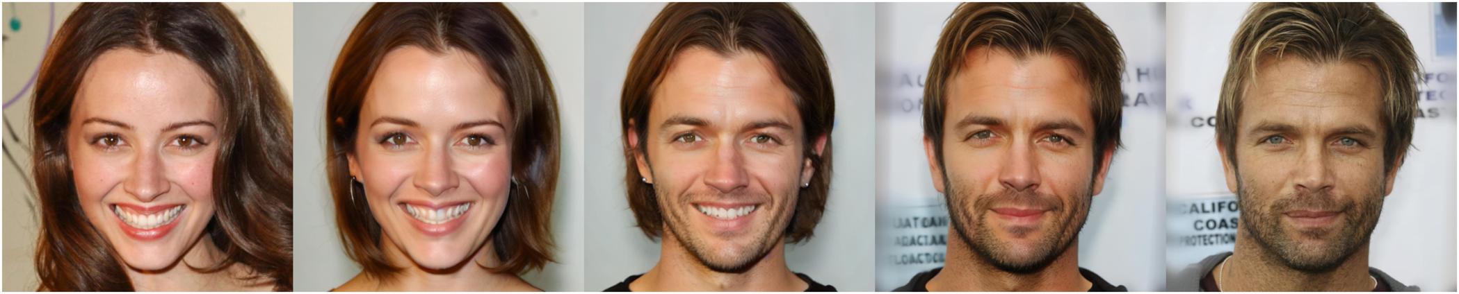
(a) CelebA-HQ female$\leftrightarrow$male

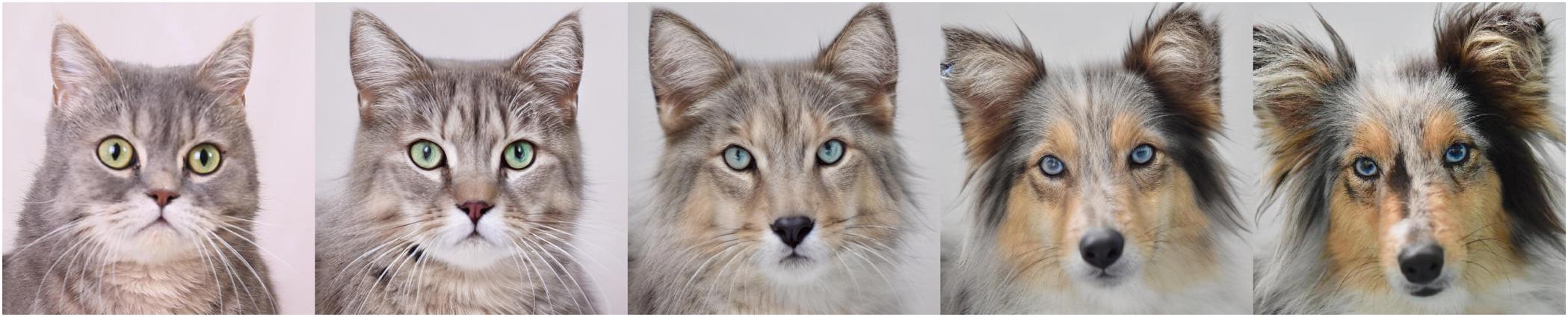
(b) AFHQ cat$\leftrightarrow$dog

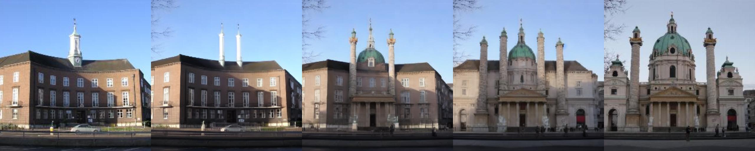
(c) LSUN church$\leftrightarrow$church

Figure 3: Examples of using IMPUS.

We perform a more detailed analysis of the proposed approach with respect to different configurations and hyperparameters. Figure 3 shows the effectiveness of our method on CelebA-HQ, AFHQ, and LSUN-Church. Total LPIPS ($\text{LPIPS}_{T}$), Max LPIPS ($\text{LPIPS}_{M}$), and FID are calculated based on the binary search sampling with a constant LPIPS interval of 0.2. PPL is with 50 intervals uniformly sampled in [0, 1].

Ablation Study on Textual Inversion. Given the importance of the text prompt for accurate conditional generation, we have claimed that suitable text embedding is critical for image morphing, which is optimized via text inversion. Alternatively, the optimized $\mathbf{e}$ could be replaced by a fine-grained human-designed text prompt.

For the benchmark datasets, we select the subset of female$\leftrightarrow$male, cat$\leftrightarrow$dog, and church$\leftrightarrow$church. We ablate textual inversion by directly using a prompt that describes the categories with results in Table 2. For female$\leftrightarrow$male, we use the prompt “a photo of woman or man”. For cat$\leftrightarrow$dog, we use the prompt “a photo of dog or cat”. In Table 2, without textual inversion, morphing sequences have a shorter and more direct path (smaller $\text{LPIPS}_{T}$ and $\text{LPIPS}_{M}$) but have an increase in reconstruction error at the endpoints. A poor reconstruction caused by the lack of textual inversion may lead to inferior morphing quality, see the Appendix for details. Thus, we claim that text inversion with a coarse initial prompt is more flexible and robust.

Table 2: Quantitative analysis on benchmark datasets. The lower the better for all metrics. For endpoint reconstruction errors, we report the mean and maximum (in parentheses) of LPIPS at the endpoints.

			Text Inversion	Adaptive Rank	Rank 4	Rank 32	$\text{LPIPS}_{T}$	$\text{LPIPS}_{M}$	FID	PPL	Endpoint Error
female$\leftrightarrow$male		✓			1.13	0.37	48.89	248.06	0.092 (0.308)
	✓	✓			1.16	0.39	48.20	238.87	0.081 (0.137)
	✓		✓		1.14	0.38	46.84	322.31	0.079 (0.132)
	✓			✓	1.09	0.37	46.12	367.70	0.080 (0.169)
cat$\leftrightarrow$dog		✓			1.61	0.50	46.28	451.85	0.125 (0.206)
	✓	✓			1.75	0.52	45.82	485.48	0.119 (0.167)
	✓		✓		1.71	0.52	48.11	613.77	0.119 (0.245)
	✓			✓	1.60	0.49	43.21	804.36	0.116 (0.190)
church$\leftrightarrow$church		✓			1.46	0.39	35.71	533.70	0.113 (0.412)
	✓	✓			1.79	0.42	36.52	1691.48	0.093 (0.248)
	✓		✓		1.85	0.42	36.02	1577.45	0.088 (0.289)
	✓			✓	1.66	0.41	34.15	2127.56	0.090 (0.266)

Table 3: Ablation study on model adaptation with text inversion. All metrics are the lower the better.

				Adaptation	$\text{LPIPS}_{T}$	$\text{LPIPS}_{M}$	FID	PPL	Endpoint Error
CelebA-HQ		1.45 $\pm$ 0.05	0.41 $\pm$ 0.01	52.76 $\pm$   4.28	196.30 $\pm$   41.78	0.192 $\pm$   0.083
	✓	1.07 $\pm$ 0.07	0.37 $\pm$ 0.01	43.59 $\pm$   5.16	201.87 $\pm$   26.34	0.083 $\pm$   0.001
AFHQ		2.27 $\pm$ 0.20	0.55 $\pm$ 0.03	42.67 $\pm$ 12.39	414.10 $\pm$   50.76	0.254 $\pm$   0.007
	✓	1.90 $\pm$ 0.18	0.54 $\pm$ 0.03	36.79 $\pm$ 11.87	679.96 $\pm$ 159.04	0.130 $\pm$   0.007
LSUN		1.94	0.40	42.48	663.33	0.184
	✓	1.79	0.42	36.52	1691.48	0.093

Ablation Study on Model Adaptation.

We further ablate model adaption and show results on CelebA-HQ, AFHQ, and LSUN in Table 3 with adaptive LoRA rank for the bottleneck constraint and textual inversion. Since AFHQ and Celeba-HQ have different settings (female$\leftrightarrow$male, dog$\leftrightarrow$dog, etc.), we report the mean and standard deviation of all settings, see the Appendix for details. Overall, model adaptation leads to more direct morphing results (smaller $\text{LPIPS}_{T}$ and $\text{LPIPS}_{M}$) and realistic images (lower FID) and lower reconstruction at endpoints. However, the higher

PPL values reflect that uniform sampling may not work well with model adaptation.

We show performance w.r.t. LoRA ranks qualitatively in Figure 4, where the selected ranks by our adaptive bottleneck constraint are in bold. From the results, the ideal rank differs for different image pairs, and our proposed rPPD can select the rank with a qualified trade-off between image quality and directness. Quantitative analysis of LoRA rank on subsets of the benchmark datasets (female$\leftrightarrow$male, cat$\leftrightarrow$dog, church$\leftrightarrow$church) is reported in Table 2. Three settings of LoRA rank are considered which are: 1) adaptive rank with bottleneck constraint, 2) rank 4, and 3) rank 32. We observe that higher LoRA ranks have better quantitative results on the benchmark dataset which is different from the conclusion we have from the internet-collected images (see Figure 4(a)-(l)). We conjecture that the scope and diversity of benchmark datasets are more limited than the internet images; thus, phenomenon such as overly blurred interpolated images occurs less likely, resulting in better performance on high LoRA ranks. Another observation is that reconstruction error at the endpoints does not decrease as the LoRA rank increases. We conjecture it is caused by the numerical error during the ODE inverse. We leave the study of these phenomena as our future work.

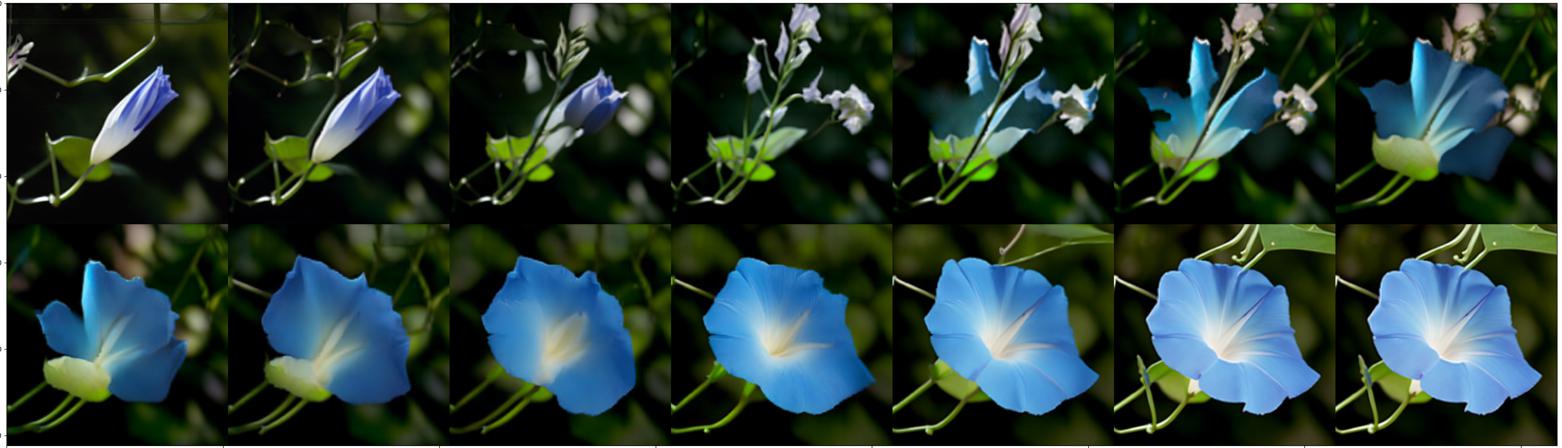
(a) Without model adaptation

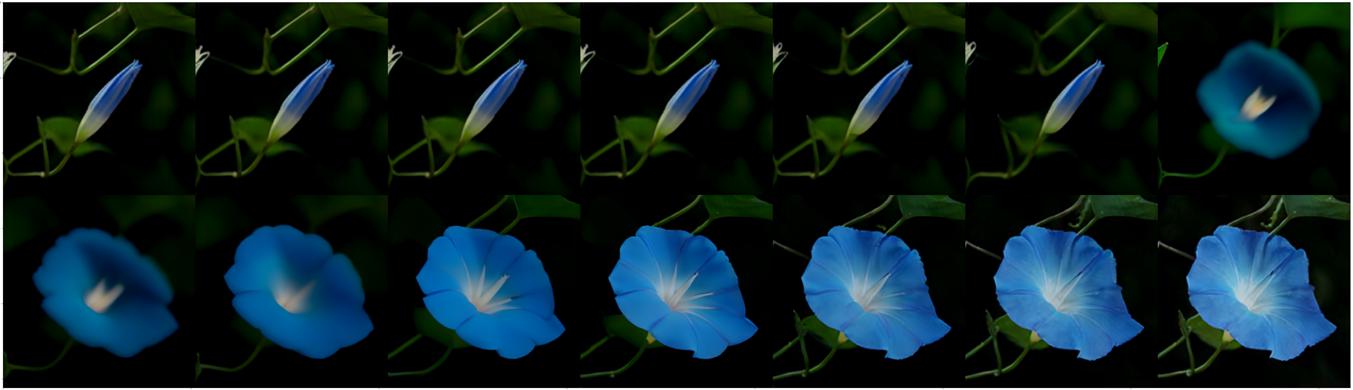
(b) Vanilla model adaptation

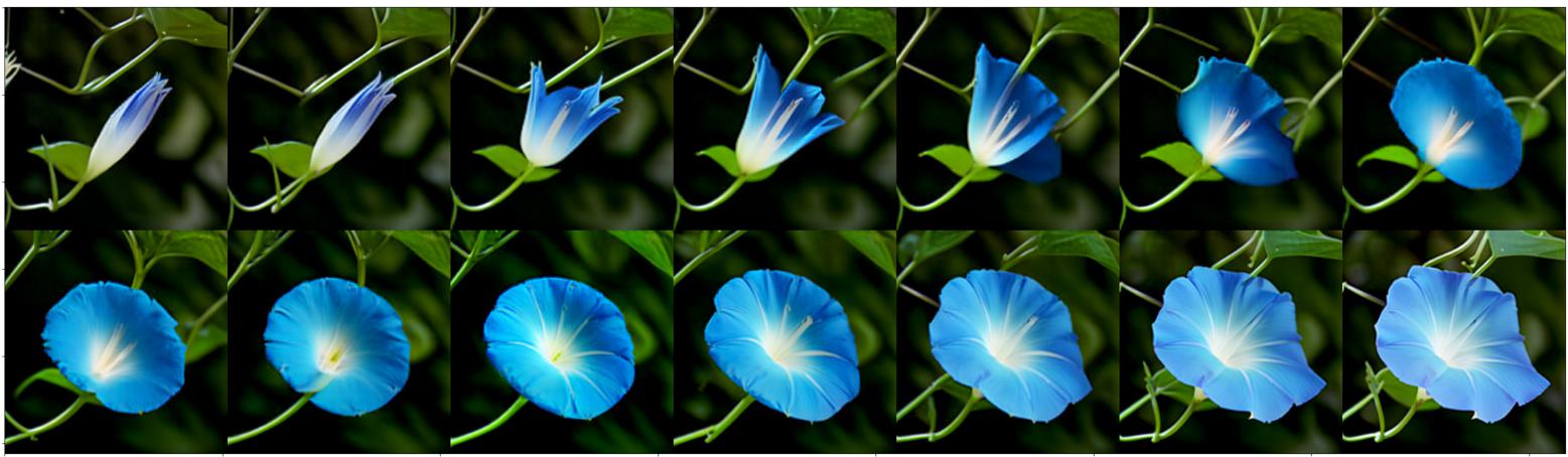
(c) LoRA with rank = 2

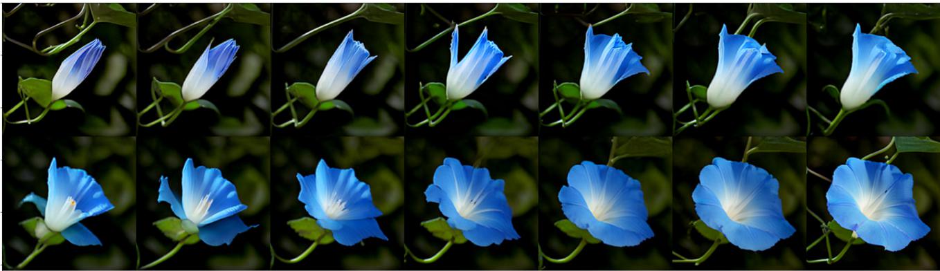
(d) LoRA with rank = 4

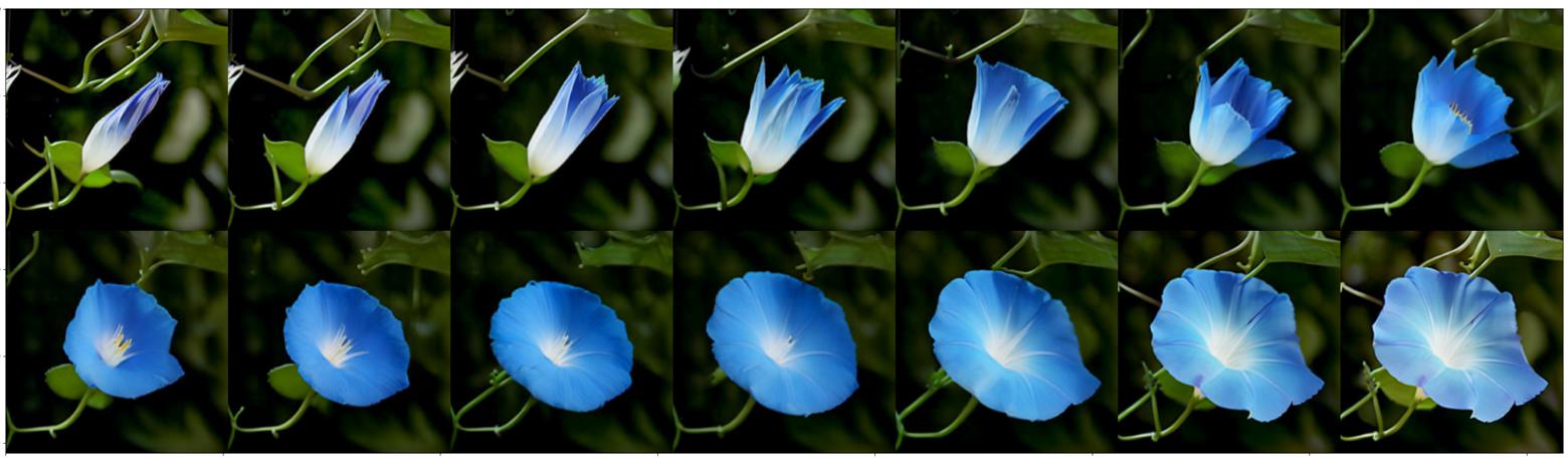
(e) LoRA with rank = 8

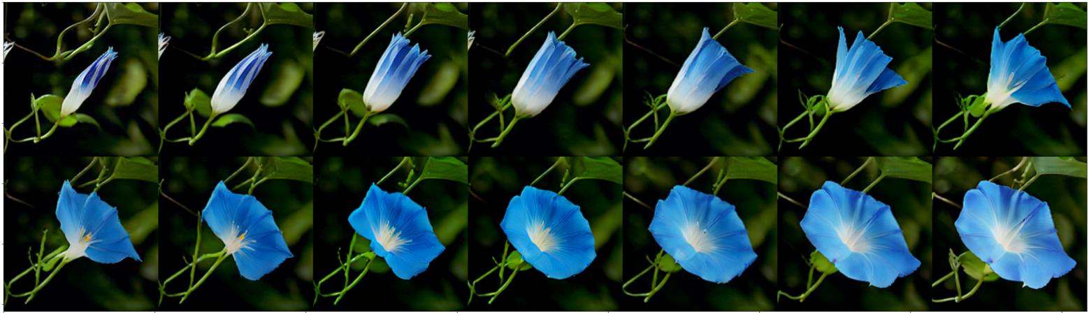
(f) LoRA with rank = 32

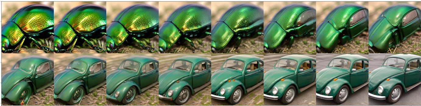
(g) LoRA with rank = 2

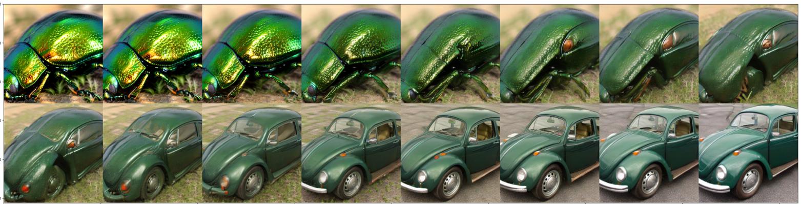
(h) LoRA with rank = 8

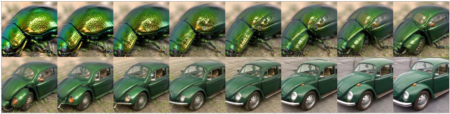
(i) LoRA with rank = 32

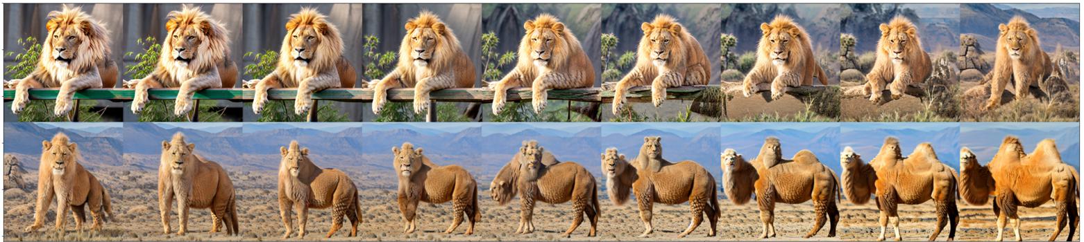
(j) LoRA with rank = 2

(k) LoRA with rank = 8

(l) LoRA with rank = 32

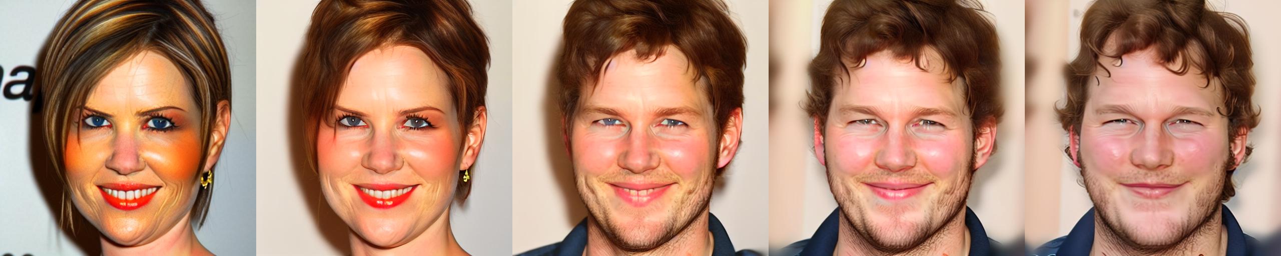
(m) Only finetune on conditioning

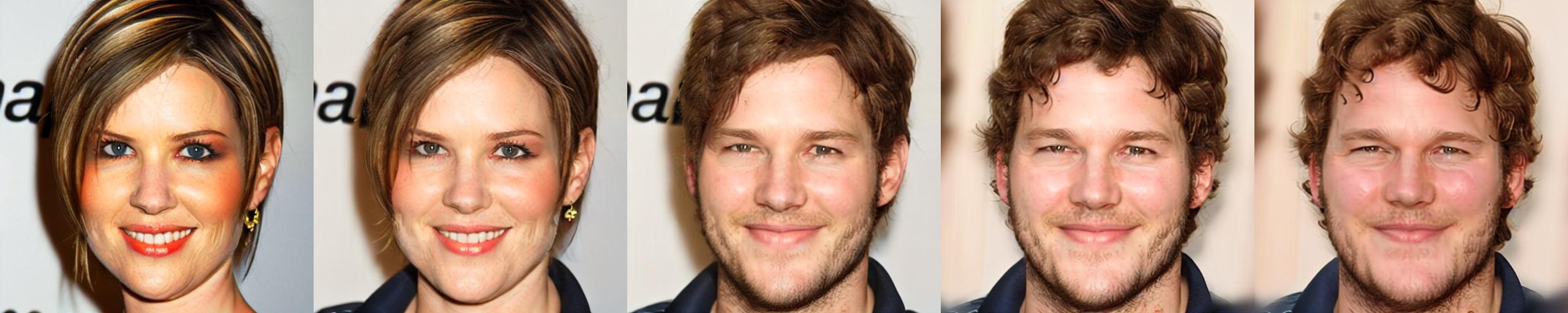
(n) Randomly discard conditioning during finetune

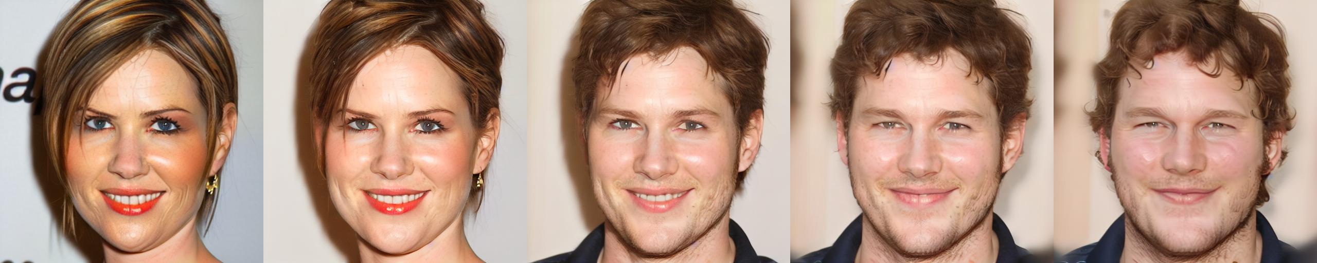
(o) Separate LoRA for unconditional estimates

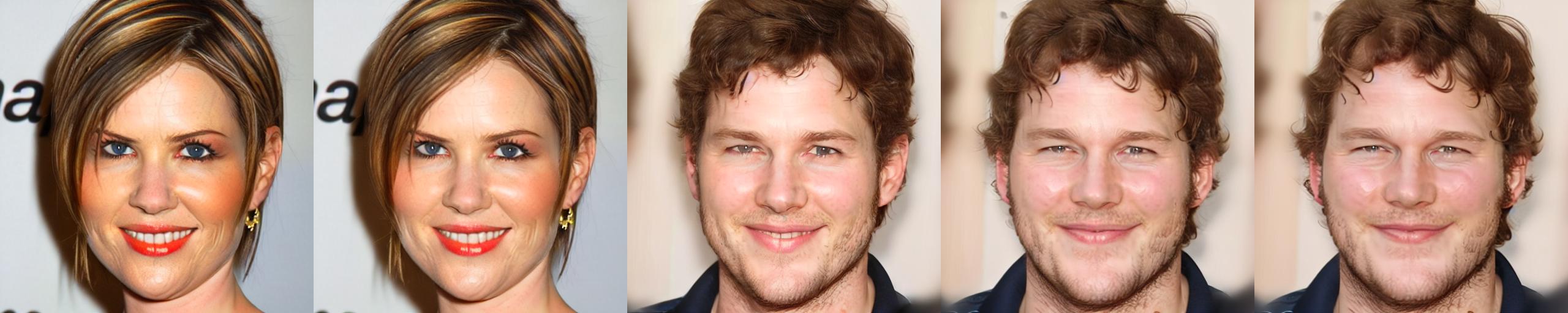
(p) Uniform space sampling

Figure 4: Ablation studies under LoRA rank, unconditional noise estimates, and sampling methods. LoRA rank: (a)-(f) intra-class on flowers with $\gamma=0.44$, (g)-(i) inter-class on beetle and car with $\gamma=0.39$, (j)-(l) inter-class on lion and camel with $\gamma=0.49$. Unconditional noise estimates: (m)-(o) Morphing sequence with the same conditional but different unconditional noise estimates. Sampling methods: (o)-(p) comparison between perceptually uniform sampling and uniform space sampling. See the Appendix for image source.

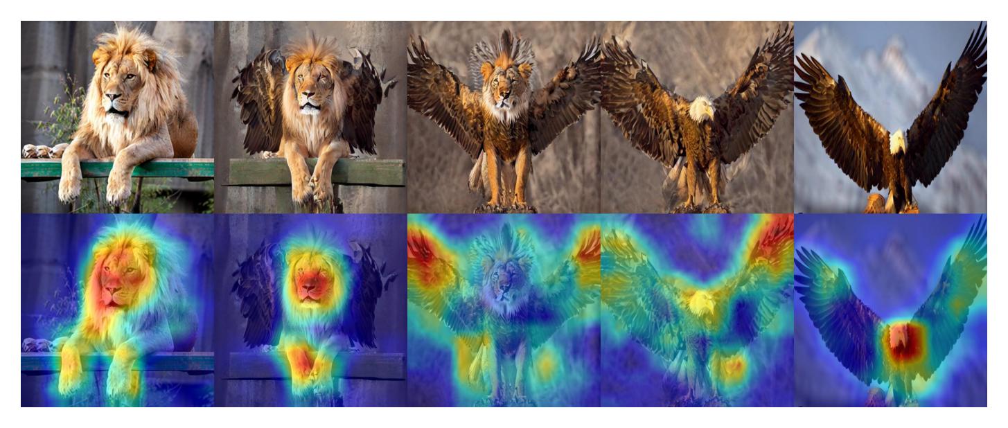
(a) GradCam on our morphing sequence

(b) Logits (x-axis: frame index)

Figure 5: Model explainability with IMPUS framework (ResNet50).

Ablation Studies on Unconditional Noise Estimates and Perceptually Uniform Sampling. We demonstrate the effects of different unconditional score estimate settings and sampling methods in Figure 4(m)-(p). If model adaptation only applies to conditional estimates, the inferior update of the unconditional estimates (due to sharing of parameters) results in a color bias, see Figure 4(m). Hence, we consider both randomly discard conditioning (Ho & Salimans, 2022) and apply a separate LoRA for unconditional score estimates.

In our experiments, applying a separate LoRA for unconditional score estimates leads to slightly higher image quality and is more robust to various guidance scales than randomly discard conditioning, see Figure 4(n)-(o). We show an example of interpolation result from uniform sampling in Figure 4(p). Compared with Figure 4(o), transitions between images in Figure 4(p) are less seamless, valid our perceptually uniform sampling technique.

5.3 Application of IMPUS to Other Tasks

Novel Sample Generation and Model Evaluation. Given images from two different categories, our morphing method is able to generate a sequence of meaningful and novel interpolated images. Figure 5 (top) shows a morphing sequence from a lion to an eagle. The interpolated images are creative and meaningful, showing the transition between the categories of two endpoints (Figure 5 (bottom)), which also shows great potential in data augmentation. Our morphing technique can be used for model evaluation and explainability. For example, the $4^{th}$ image of the morphing sequence looks like an eagle, but the highest logit is prairie fowl. With GradCAM (Selvaraju et al., 2017), the background can distinguish the prairie fowl from the eagle.

Video Interpolation. Our morphing tools can also be directly applied for video interpolation. In Figure 6, given the start and end frames, we can generate realistic interpolated frames. We claim that more interpolated images can further boost our performance for video interpolation.

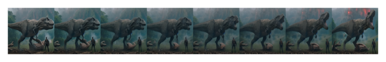
Figure 6: Video interpolation with IMPUS on a movie clip of Jurassic World (Bayona, 2018) and a running dog from YouTube (EpicSlowMotionDog, 2013).

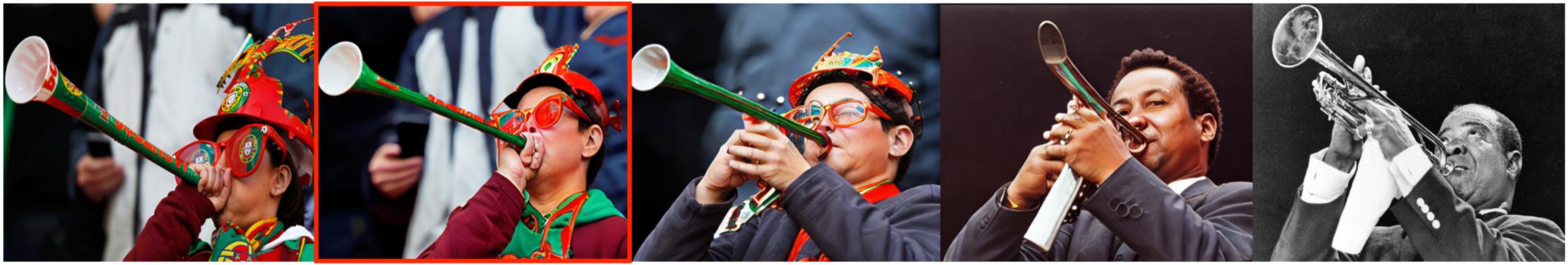
Figure 7: Failure cases of IMPUS.

6 Conclusion

In this work, we introduce a diffusion-based image morphing approach with perceptually-uniform sampling, namely IMPUS, to generate smooth, realistic, and direct interpolated images given an image pair. We show that our model adaptation with an adaptive bottleneck constraint can suppress inferior transition variations and increase the image diversity with a specific directness. Our experiments validate that our approach can generate high-quality morphs and shows its potential for data augmentation, model explainability and video interpolation. Although IMPUS achieves high-quality morphing results, abrupt transitions occur when the given images have a significant semantic difference, see Figure 7(a). In cases like Figure 7(b), our approach generates incorrect hands, which is common for diffusion models. Hence, more investigations are desirable in our future work.

Appendix A Appendix

A.1 preliminary On Diffusion Models

Denoising Diffusion Probabilistic Models (DDPM). DDPM uncovers the probability density function of an underlined data manifold via maximizing the variational evidence lower bound (ELBO) of data likelihood, i.e.,

$$\max_{\theta}\mathbb{E}_{q\left({\mathbf{x}}_{0}\right)}\left[\log p_{\theta}\left({\mathbf{x}}_{0}\right)\right]\geq\max_{\theta}\mathcal{L}_{\mathrm{VLB}}=\max_{\theta}\mathbb{E}_{q\left({\mathbf{x}}_{0:T}\right)}\left[\log\frac{p_{\theta}\left({\mathbf{x}}_{0:T}\right)}{q\left({\mathbf{x}}_{1:T}\mid{\mathbf{x}}_{0}\right)}\right]\ .$$ (11)

Given the variational lower bound in Eq. (11), DDPM is defined as a Markovian process, i.e., $p_{\theta}\left({\mathbf{x}}_{0:T}\right):=p_{\theta}^{(T)}\left({\mathbf{x}}_{T}\right)\prod_{t=1}^{T}p_{\theta}^{(t)}\left({\mathbf{x}}_{t-1}\mid{\mathbf{x}}_{t}\right)$, $q\left({\mathbf{x}}_{1:T}\mid{\mathbf{x}}_{0}\right):=\prod_{t=1}^{T}q^{(t)}\left({\mathbf{x}}_{t}\mid{\mathbf{x}}_{t-1}\right)$. The variational lower bound is decomposed into

$$L_{\mathrm{VLB}} =-\mathbb{E}_{q\left({\mathbf{x}}_{0:T}\right)}[\underbrace{D_{\mathrm{KL}}\left(q\left({\mathbf{x}}_{T}\mid{\mathbf{x}}_{0}\right)\|p_{\theta}\left({\mathbf{x}}_{T}\right)\right)}_{L_{T}}$$ (12)

$$-\sum_{t=2}^{T}\underbrace{D_{\mathrm{KL}}\left(q\left({\mathbf{x}}_{t-1}\mid{\mathbf{x}}_{t},{\mathbf{x}}_{0}\right)\|p_{\theta}\left({\mathbf{x}}_{t-1}\mid{\mathbf{x}}_{t}\right)\right)}_{L_{t-1}}+\underbrace{\log p_{\theta}\left({\mathbf{x}}_{0}\mid{\mathbf{x}}_{1}\right)}_{L_{0}}]\ ,$$

where $q\left({\mathbf{x}}_{t}\mid{\mathbf{x}}_{t-1}\right):=\mathcal{N}\left({\mathbf{x}}_{t};\sqrt{\frac{\alpha_{t}}{\alpha_{t-1}}}{\mathbf{x}}_{t-1},\left(1-\frac{\alpha_{t}}{\alpha_{t-1}}\right)\bm{I}\right)$, the accumulative transition distribution is defined as

$$q\left({\mathbf{x}}_{t}\mid{\mathbf{x}}_{0}\right):=\int q\left({\mathbf{x}}_{1:t}\mid{\mathbf{x}}_{0}\right)\mathrm{d}{\mathbf{x}}_{1:(t-1)}=\mathcal{N}\left({\mathbf{x}}_{t};\sqrt{\alpha_{t}}{\mathbf{x}}_{0},\left(1-\alpha_{t}\right){\mathbf{I}}\right)\ .$$ (13)

The reverse diffusion process is defined by the Bayes rule, i.e.,

$$q\left({\mathbf{x}}_{t-1}\mid{\mathbf{x}}_{t},{\mathbf{x}}_{0}\right)=q\left({\mathbf{x}}_{t}\mid{\mathbf{x}}_{t-1},{\mathbf{x}}_{0}\right)\frac{q\left({\mathbf{x}}_{t-1}\mid{\mathbf{x}}_{0}\right)}{q\left({\mathbf{x}}_{t}\mid{\mathbf{x}}_{0}\right)}\ .$$ (14)

Denoising Diffusion Implicit Models (DDIM).

In this paper, we use a DDIM (Song et al., 2020a), where given the same transition rule in Eq. (13), the reverse process $q\left({\mathbf{x}}_{t-\Delta t}\mid{\mathbf{x}}_{t},{\mathbf{x}}_{0}\right)$ is define by the following equality

$$\int q\left({\mathbf{x}}_{t-\Delta t}\mid{\mathbf{x}}_{t},{\mathbf{x}}_{0}\right)q\left({\mathbf{x}}_{t}\mid{\mathbf{x}}_{0}\right)d{\mathbf{x}}_{t}=q\left({\mathbf{x}}_{t-\Delta t}\mid{\mathbf{x}}_{0}\right)\ .$$ (15)

which leads to a larger solution set than DDPM. For a sample ${\mathbf{x}}_{t}$, the reverse step is defined as follows with a random variable $\sigma_{t}$

$${\mathbf{x}}_{t-\Delta t}=\sqrt{\alpha_{t-\Delta t}}\underbrace{\left(\frac{{\mathbf{x}}_{t}-\sqrt{1-\alpha_{t}}\epsilon_{\theta}^{(t)}\left({\mathbf{x}}_{t}\right)}{\sqrt{\alpha_{t}}}\right)}_{\text{``predicted }{\mathbf{x}}_{0}"}+\underbrace{\sqrt{1-\alpha_{t-\Delta t}-\sigma_{t}^{2}}\cdot\epsilon_{\theta}^{(t)}\left({\mathbf{x}}_{t}\right)}_{\text{``direction pointing to }{\mathbf{x}}_{t}"}+\underbrace{\sigma_{t}\epsilon_{t}}_{\text{``random noise"}}\ .$$ (16)

By setting the free variable $\sigma_{t}$ in Eq. (16) as $0$, we have a deterministic generative pass as follows

$$\frac{{\mathbf{x}}_{t-\Delta t}}{\sqrt{\alpha_{t-\Delta t}}}=\frac{{\mathbf{x}}_{t}}{\sqrt{\alpha_{t}}}+\left(\sqrt{\frac{1-\alpha_{t-\Delta t}}{\alpha_{t-\Delta t}}}-\sqrt{\frac{1-\alpha_{t}}{\alpha_{t}}}\right)\epsilon_{\theta}^{(t)}\left({\mathbf{x}}_{t}\right)\ ,$$ (17)

which can be seen as the discretization of a continuous-time ODE (Song et al., 2020a)

$$\lim_{\Delta t\rightarrow 0}\frac{{\mathbf{x}}_{t}}{\sqrt{\alpha_{t}}}-\frac{{\mathbf{x}}_{t-\Delta t}}{\sqrt{\alpha_{t-\Delta t}}} =\lim_{\Delta t\rightarrow 0}\left(\sqrt{\frac{1-\alpha_{t}}{\alpha_{t}}}-\sqrt{\frac{1-\alpha_{t-\Delta t}}{\alpha_{t-\Delta t}}}\right)\epsilon_{\theta}^{(t)}\left({\mathbf{x}}_{t}\right)\ ,$$ (18)

$$\mathrm{d}\overline{{\mathbf{x}}}(t) =\epsilon_{\theta}^{(t)}\left(\frac{\overline{{\mathbf{x}}}(t)}{\sqrt{\sigma^{2}(t)+1}}\right)\mathrm{d}\sigma(t)\ ,$$

where $\overline{{\mathbf{x}}}(t)=\frac{{\mathbf{x}}_{t}}{\sqrt{\alpha_{t}}}$ and $\sigma(t)=\sqrt{\frac{1-\alpha_{t}}{\alpha_{t}}}$.

A.2 Further Discussion on comparison with Wang & Golland (2023)

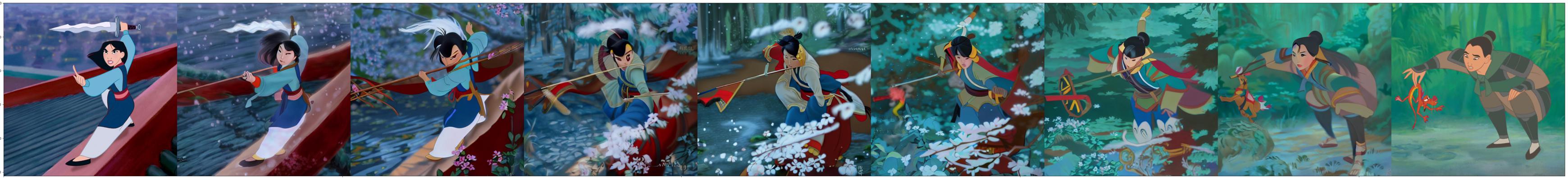
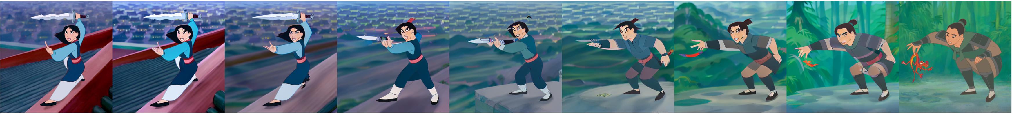
Figure 8: Compared with Wang & Golland (2023), our approach does not require extra guidance signals to achieve consistency in pose variation nor fine-grained text prompts. Together with the proposed model adaptation strategy, our approach demonstrates superior image morphing performance.

(a) Interpolation result of Wang & Golland (2023) without (left) and with (right) pose guidance

(b) Our image morphing results with generic text prompts (left) and model adaptation (right)

We find three major differences of Wang & Golland (2023) with our work: 1) task definition - Wang & Golland (2023) works on “image interpolation” , where they focus on novel image creation with the constraint of realism smoothness. However, we argue that the definition for “novel image generation” is ambiguous and can hardly be quantitatively analyzed. Our work instead focuses on image morphing, which has three clear and measurable targets: smoothness, realism, and directness 2) flexibility in prompt engineering - Wang & Golland (2023) relies on a careful and fine-grained selection of initial textual prompts, while our work can achieve solid morphing results with coarsely selected initial prompts, e.g., for boundary samples in Fig. 8, Wang & Golland (2023) uses two detailed prompts: $<$HDR photo of a person practicing martial arts, crisp, smooth, photorealistic, high-quality wallpaper, ultra HD, detailed$>$ and $<$HDR photo of a person leaning over, crisp, smooth, high-quality wallpaper$>$, while we use a coarse prompt $<$a photo of a cartoonish character$>$; 3) inputs w.t. inconsistent pose - as shown in Fig. 8, to handle image pair with inconsistent poses, Wang & Golland (2023) relies on extra supervision signal from a human pose estimation model. Differently, our work can obtain high-quality & consistent morphing results w.o. requiring any extra supervision beyond the source diffusion model itself. We note that, in the original paper of Wang & Golland (2023), 26 pairs of images are claimed to be used, but there is access to only 25 pairs as provided in their public Repository https://github.com/clintonjwang/ControlNet. We present additional comparison with Wang & Golland (2023) in Fig. 9

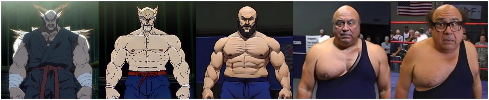
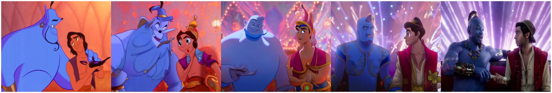
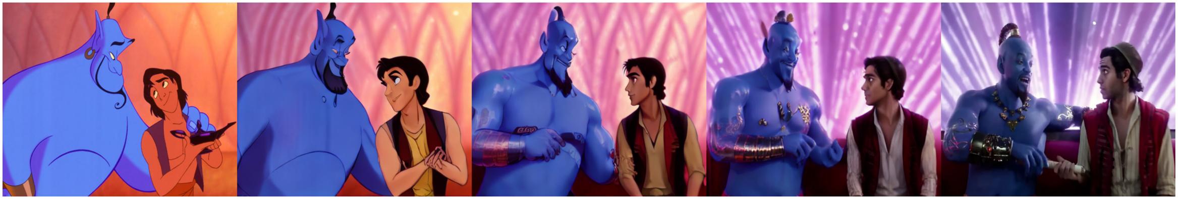
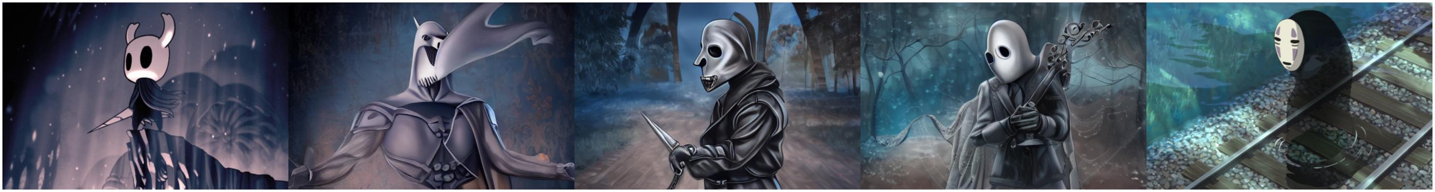
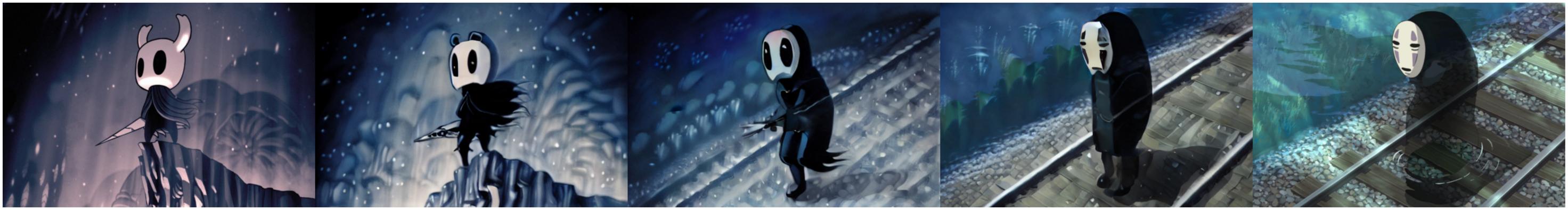
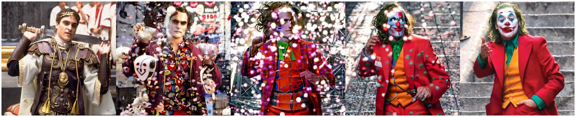
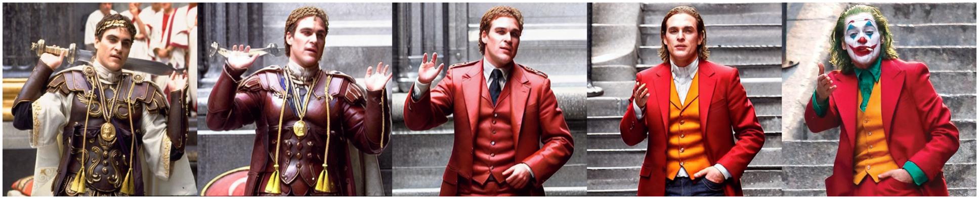
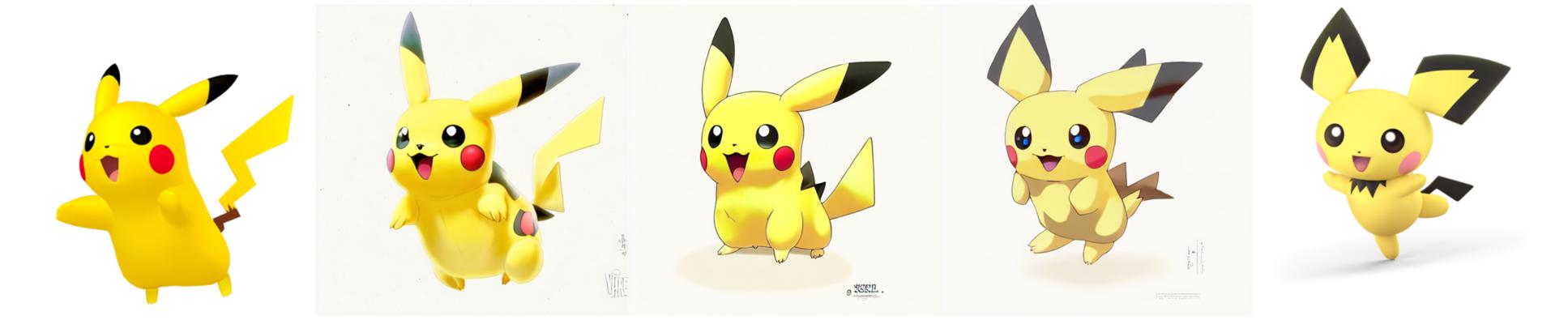
(a) Wang & Golland (2023)

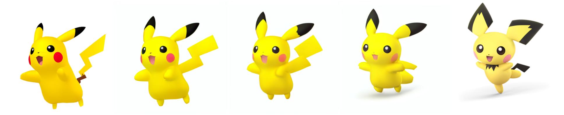
(b) Ours

Figure 9: Additional comparison results.

A.3 Further Implementation Details

For all the experiments, we use use a latent space diffusion model (Rombach et al., 2022), with pre-trained weights from Stable-Diffusion-v-1-4 . Textual inversion is trained with AdamW optimizer (Loshchilov & Hutter, 2018), and the learning rate is set as 0.002 for 2500 steps. For the benchmark dataset, we perform text inversion for 1000 steps. LoRA is trained with Adam optimizer (Kingma & Ba, 2014), and the learning rate is set as 0.001.

Perceptually Uniform Sampling

The overall process of our proposed perceptually-uniform sampling method based on binary search is presented in Algorithm 1.

Algorithm 1 Perceptually-Uniform Sampling with constant LPIPS

1:$\alpha_{start}$: starting alpha value; $\alpha_{end}$: ending alpha value; $\delta$: difference between consecutive sampling images, $\epsilon_{tol}$: error tolerance for binary search

2:$\bm{\alpha}_{list}$: list of alpha.

3:procedure BinarySearch($\alpha_{start},\alpha_{end},\delta_{lpips},\epsilon_{tol}$)

4:     $\bm{\alpha}_{list}\leftarrow[\alpha_{start}]$, $\alpha_{cur}\leftarrow\alpha_{start}$ $\triangleright$ Initialization

5:     while $D(\alpha_{cur},\alpha_{end})>\delta$ do $\triangleright$ Binary search of constant LPIPS

6:         $\alpha_{t1}\leftarrow\alpha_{cur}$, $\alpha_{t2}\leftarrow\alpha_{end}$, $\alpha_{mid}\leftarrow\frac{\alpha_{t1}+\alpha_{t2}}{2}$

7:         while $\big{|}\operatorname{LPIPS}({\mathbf{x}}^{(\alpha_{cur})},{\mathbf{x}}^{(\alpha_{mid})})-\delta\big{|}>\epsilon_{tol}$ do

8:              if $\operatorname{LPIPS}({\mathbf{x}}^{(\alpha_{cur})},{\mathbf{x}}^{(\alpha_{mid})})>\delta$ then

9:                  $\alpha_{t2}\leftarrow\frac{\alpha_{t1}+\alpha_{t2}}{2}$

10:              else

11:                  $\alpha_{t1}\leftarrow\frac{\alpha_{t1}+\alpha_{t2}}{2}$               

12:              $\alpha_{mid}\leftarrow\frac{\alpha_{t1}+\alpha_{t2}}{2}$          

13:         $\alpha_{cur}\leftarrow\alpha_{mid}$, $\bm{\alpha}_{list}\leftarrow\bm{\alpha}_{list}\bigcup\alpha_{cur}$ $\triangleright$ Append alpha to the list      

14:     $\bm{\alpha}_{list}\leftarrow\bm{\alpha}_{list}\bigcup\alpha_{end}$ $\triangleright$ Append the ending alpha

15:     return $\bm{\alpha}_{list}$

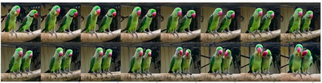
Figure 10: Interpolation of two video frames - teleporting parrot.

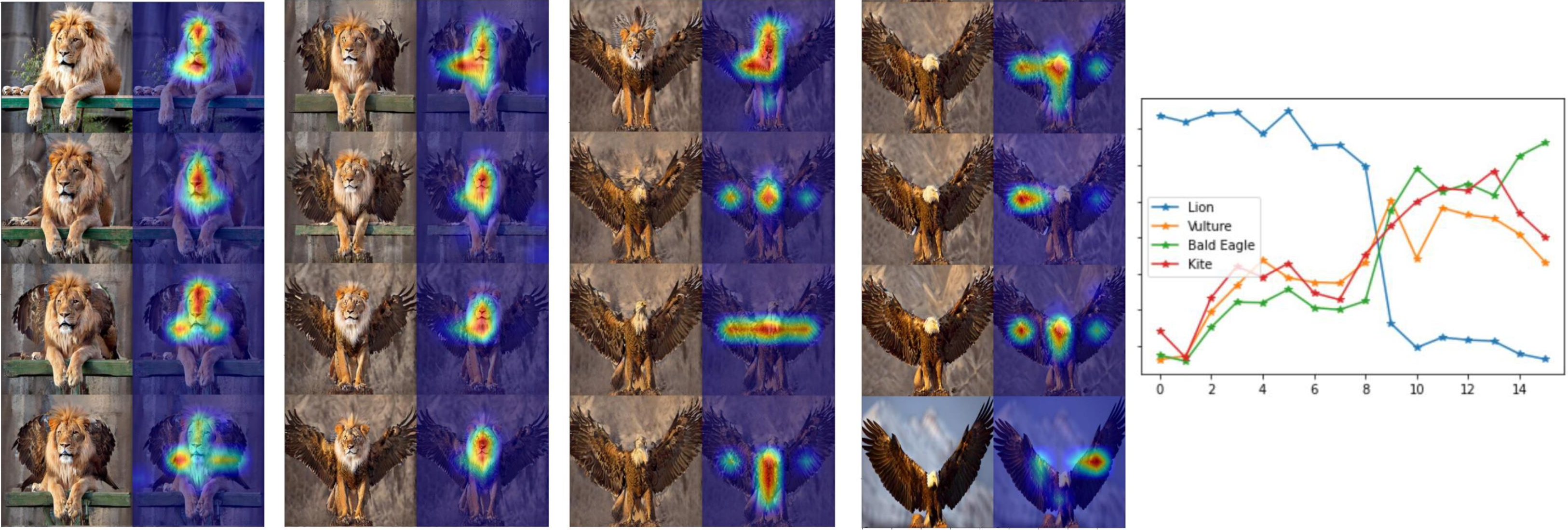
Figure 11: Model explainability with our morphing tool (SwinT).

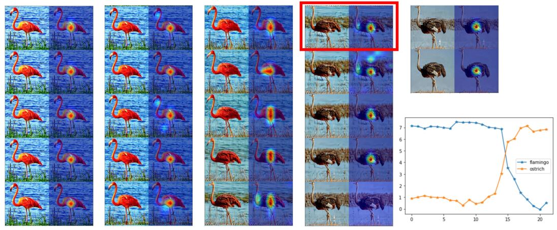
Figure 12: Model explainability with our morphing tool (SwinT).

Quality Boosting

Convex CFG Scheduling. Although the interpolation between initial states and inverted textual embeddings can facilitate a smooth connection between inputs, however, we observe that the intermediate samples in the morphing path often show lower saturation than the ones near the boundaries. Intuitively, after model adaptation, the overall probability densities $p_{\theta}({\mathbf{x}}_{t},t)$ would concentrate more on the boundary samples, leading to lower density for regions in between. In order to provide extra guidance cues to guide the generation of intermediate samples via enforcing a larger density ratio $p_{\theta}({\mathbf{x}}_{t},t|e)/p_{\theta}({\mathbf{x}}_{t},t)$, we propose a convex CFG scheduling in the form of $w_{\alpha}=w_{max}-2(w_{max}-w_{min})|\alpha-0.5|$, which can boost the generation quality for intermediate samples as shown in Fig. 13.

Stochasticity Boosting.

For semantically distinct input pairs, artifacts may appear in details of the intermediate morphing results, where one possible cause is ODE sampler with limited time steps. As shown in prior works (Karras et al., 2022; Kwon et al., 2023), stochastic diffusion samplers often show improved quality than deterministic ones. Taking the reverse DDIM process in Eq. (16) as an example, a stochastic sampler sets a positive $\sigma_{t}$, which requires extra “denoising” by the diffusion model for newly introduced Gaussian noises on top of “denoising” for initial noise, which may also correct the prediction errors from earlier denoising steps. However, setting a positive $\sigma_{t}$ throughout the denoising process may fail to provide a faithful preservation of input content. To find a balance, using a total of 16-time steps, we find that setting $\sigma_{t}$ as 0 for the initial 6 steps and setting $\sigma_{t}$ as 1 for the rest 10 steps can faithfully retain the content from inputs while correcting some artifacts as shown in Fig. 13.

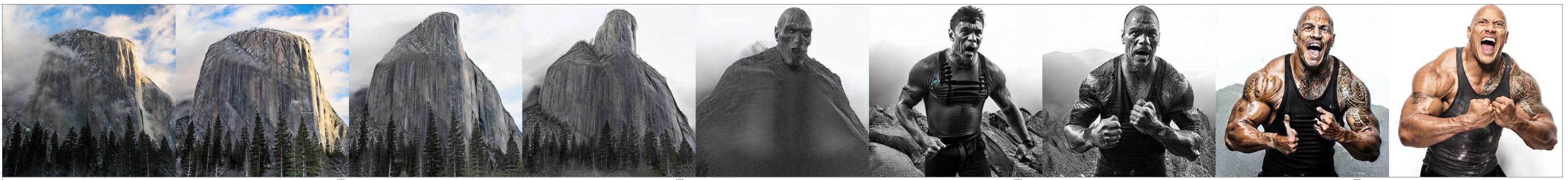
(a) Morphing result of our work w.t. fixed CFG.

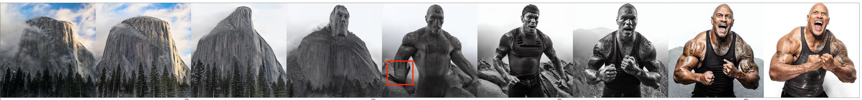
(b) Result w.o. stochasticity boosting.

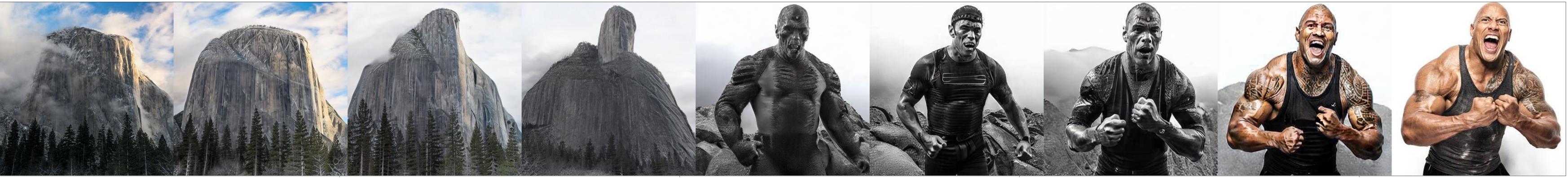
(c) Results of our w.t. quality boosting.

Figure 13: Illustration on the effect of quality boosting.

Ablation Study on CFG.

We also study the effects of different hyperparameters, such as the scale of classifier-free guidance. We observe that inversion-only morphing requires a stronger CFG scale, while inversion with adaptation requires less guidance. In most situations, a large CFG scale can degrade the morphing quality and lead to a longer morphing sequence. We provide ablation studies of CFG on total LPIPS (Table. 4), Max LPIPS (Table. 5), FID (Table. 6) and PPL (Table. 7).

A.4 Failure case without textual inversion

In our work, textual inversion is performed on the embedding of a coarsely initialized prompt. Alternatively, the optimized embedding could be replaced by a fine-grained human-designed text prompt. We find that using an appropriate prompt shared by two images can improve the smoothness of the morphing path without loss of image quality (see the first example in Fig. 14). However, for an arbitrary pair of images, it is usually difficult to choose such an ideal prompt (see the second example in Fig. 14 for failure cases where a human-labeled prompt is not informative enough to reconstruct given images, resulting in inferior performance). Instead, our textual inversion with a coarse initial prompt is more flexible and robust.

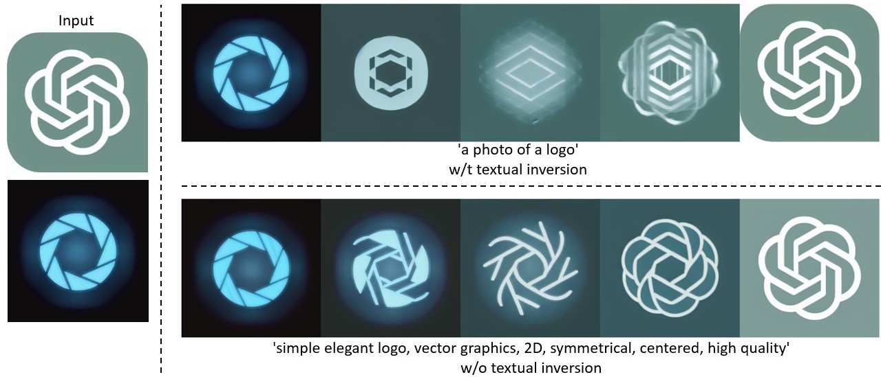
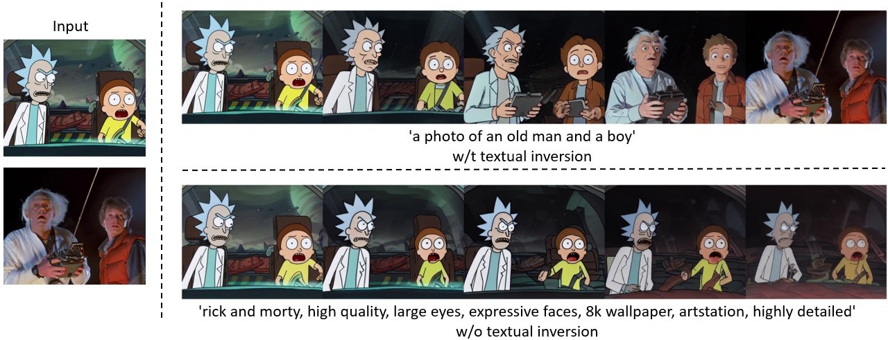
Figure 14: Results w.o. textual inversion using detailed prompt. In the first example where an appropriate description is selected to be shared by two images, the morphing path shows improved directness w.o. textual inversion. In the example below, an inappropriate prompt leads to an unfaithful reconstruction of inputs and downgraded quality.

A.5 Quantitative Results

We provide detailed tables in this section. Different scales of guidance are considered: (1) CFG1: 1.5-2, (2) CFG2: 2-3, (3) CFG3: 3-4, and (4) CFG4: 4-5.

Table 4: Mean and standard deviation of total LPIPS.

dataset inv only CFG1 inv only CFG2 inv only CFG3 inv only CFG4 inv+adapt CFG1 inv+adapt CFG2 adapt only CFG1 adapt only CFG2 male $\leftrightarrow$ male 1.38 $\pm$ 0.36 1.80 $\pm$ 0.66 1.51 $\pm$ 0.33 1.97 $\pm$ 0.40 1.02 $\pm$ 0.19 1.12 $\pm$ 0.20 NaN NaN female $\leftrightarrow$ female 1.45 $\pm$ 0.53 1.63 $\pm$ 0.43 1.42 $\pm$ 0.28 1.84 $\pm$ 0.36 1.03 $\pm$ 0.16 1.16 $\pm$ 0.21 NaN NaN female $\leftrightarrow$ male 1.50 $\pm$ 0.26 1.82 $\pm$ 0.38 1.60 $\pm$ 0.27 2.11 $\pm$ 0.30 1.16 $\pm$ 0.16 1.31 $\pm$ 0.18 1.13 $\pm$ 0.17 1.27 $\pm$ 0.18 cat $\leftrightarrow$ cat 2.23 $\pm$ 0.62 2.70 $\pm$ 0.59 2.79 $\pm$ 0.81 3.39 $\pm$ 0.92 1.87 $\pm$ 0.44 2.18 $\pm$ 0.53 NaN NaN dog $\leftrightarrow$ dog 2.59 $\pm$ 0.60 3.31 $\pm$ 0.77 3.06 $\pm$ 0.75 3.89 $\pm$ 1.03 2.20 $\pm$ 0.41 2.51 $\pm$ 0.49 NaN NaN wild 2.20 $\pm$ 0.40 2.70 $\pm$ 0.62 2.58 $\pm$ 0.60 3.23 $\pm$ 0.76 1.78 $\pm$ 0.31 2.06 $\pm$ 0.37 NaN NaN cat $\leftrightarrow$ dog 2.04 $\pm$ 0.40 2.57 $\pm$ 0.42 2.62 $\pm$ 0.60 3.31 $\pm$ 0.86 1.75 $\pm$ 0.24 2.10 $\pm$ 0.40 1.61 $\pm$ 0.25 1.83 $\pm$ 0.26 church $\leftrightarrow$ church 1.94 $\pm$ 0.44 2.58 $\pm$ 0.54 2.68 $\pm$ 0.56 3.76 $\pm$ 0.78 1.79 $\pm$ 0.34 2.26 $\pm$ 0.57 NaN NaN

Table 5: Mean and standard deviation of max LPIPS.

dataset inv only CFG1 inv only CFG2 inv only CFG3 inv only CFG4 inv+adapt CFG1 inv+adapt CFG2 adapt only CFG1 adapt only CFG2 male 0.40 $\pm$ 0.06 0.43 $\pm$ 0.06 0.41 $\pm$ 0.05 0.43 $\pm$ 0.05 0.36 $\pm$ 0.05 0.38 $\pm$ 0.05 NaN NaN female 0.41 $\pm$ 0.06 0.43 $\pm$ 0.04 0.40 $\pm$ 0.05 0.43 $\pm$ 0.05 0.37 $\pm$ 0.04 0.38 $\pm$ 0.04 NaN NaN female male 0.42 $\pm$ 0.04 0.45 $\pm$ 0.03 0.42 $\pm$ 0.04 0.45 $\pm$ 0.04 0.39 $\pm$ 0.04 0.40 $\pm$ 0.03 0.37 $\pm$ 0.04 0.39 $\pm$ 0.04 cat 0.57 $\pm$ 0.06 0.60 $\pm$ 0.06 0.59 $\pm$ 0.07 0.61 $\pm$ 0.07 0.55 $\pm$ 0.07 0.56 $\pm$ 0.07 NaN NaN dog 0.59 $\pm$ 0.05 0.62 $\pm$ 0.04 0.61 $\pm$ 0.05 0.63 $\pm$ 0.04 0.59 $\pm$ 0.05 0.59 $\pm$ 0.05 NaN NaN wild 0.54 $\pm$ 0.04 0.56 $\pm$ 0.04 0.55 $\pm$ 0.04 0.58 $\pm$ 0.04 0.51 $\pm$ 0.04 0.51 $\pm$ 0.04 NaN NaN cat dog 0.53 $\pm$ 0.05 0.57 $\pm$ 0.04 0.56 $\pm$ 0.04 0.59 $\pm$ 0.04 0.52 $\pm$ 0.04 0.54 $\pm$ 0.03 0.50 $\pm$ 0.04 0.50 $\pm$ 0.03 church 0.40 $\pm$ 0.03 0.43 $\pm$ 0.04 0.44 $\pm$ 0.04 0.46 $\pm$ 0.04 0.42 $\pm$ 0.04 0.43 $\pm$ 0.04 NaN NaN

Table 6: Mean and standard deviation of FID.

dataset inv only CFG1 inv only CFG2 inv only CFG3 inv only CFG4 inv+adapt CFG1 inv+adapt CFG2 adapt only CFG1 adapt only CFG2 male 57.58 $\pm$ 0.32 70.06 $\pm$ 0.39 63.26 $\pm$ 0.36 72.49 $\pm$ 0.42 46.19 $\pm$ 0.25 49.53 $\pm$ 0.27 NaN NaN female 47.17 $\pm$ 0.29 47.59 $\pm$ 0.30 46.66 $\pm$ 0.31 53.99 $\pm$ 0.36 36.39 $\pm$ 0.23 37.88 $\pm$ 0.23 NaN NaN female male 53.55 $\pm$ 0.29 61.39 $\pm$ 0.35 59.41 $\pm$ 0.33 67.82 $\pm$ 0.38 48.20 $\pm$ 0.25 48.69 $\pm$ 0.26 48.89 $\pm$ 0.25 50.92 $\pm$ 0.26 cat 36.53 $\pm$ 0.26 39.49 $\pm$ 0.29 40.75 $\pm$ 0.30 45.87 $\pm$ 0.34 32.09 $\pm$ 0.21 35.00 $\pm$ 0.22 NaN NaN dog 61.45 $\pm$ 0.32 72.59 $\pm$ 0.38 55.17 $\pm$ 0.34 61.73 $\pm$ 0.39 49.62 $\pm$ 0.28 50.15 $\pm$ 0.28 NaN NaN wild 23.69 $\pm$ 0.20 30.33 $\pm$ 0.24 23.28 $\pm$ 0.22 27.31 $\pm$ 0.25 19.61 $\pm$ 0.17 20.11 $\pm$ 0.18 NaN NaN cat dog 56.13 $\pm$ 0.30 63.61 $\pm$ 0.36 51.50 $\pm$ 0.33 56.46 $\pm$ 0.38 45.82 $\pm$ 0.26 49.12 $\pm$ 0.29 46.28 $\pm$ 0.26 48.57 $\pm$ 0.29 church 43.64 $\pm$ 0.42 44.61 $\pm$ 0.44 42.48 $\pm$ 0.44 45.35 $\pm$ 0.50 36.52 $\pm$ 0.36 38.87 $\pm$ 0.39 NaN NaN

Table 7: Mean and standard deviation of PPL.

dataset inv only CFG1 inv only CFG2 inv only CFG3 inv only CFG4 inv+adapt CFG1 inv+adapt CFG2 adapt only CFG1 adapt only CFG2 male 187.80 $\pm$ 464.17 293.92 $\pm$ 712.75 583.94 $\pm$ 1816.54 877.37 $\pm$ 2765.22 187.10 $\pm$ 423.31 323.73 $\pm$ 731.63 NaN NaN female 149.92 $\pm$ 275.70 258.72 $\pm$ 628.28 505.10 $\pm$ 1381.98 591.45 $\pm$ 2851.81 179.65 $\pm$ 375.86 305.35 $\pm$ 694.54 NaN NaN female male 251.19 $\pm$ 480.31 421.73 $\pm$ 1228.64 901.66 $\pm$ 4177.53 980.52 $\pm$ 3007.18 238.87 $\pm$ 557.78 394.47 $\pm$ 916.87 248.06 $\pm$ 766.20 381.27 $\pm$ 1616.40 cat 432.71 $\pm$ 823.13 876.83 $\pm$ 2735.96 1451.21 $\pm$ 3078.00 1977.90 $\pm$ 5408.94 710.25 $\pm$ 1600.53 1196.90 $\pm$ 2326.12 NaN NaN dog 475.55 $\pm$ 817.85 1053.61 $\pm$ 2423.10 2005.83 $\pm$ 4091.21 2534.77 $\pm$ 6712.03 918.50 $\pm$ 2246.47 1674.60 $\pm$ 4529.26 NaN NaN wild 412.65 $\pm$ 713.96 747.22 $\pm$ 1327.47 1383.24 $\pm$ 3071.43 1395.23 $\pm$ 3781.30 605.59 $\pm$ 1459.92 1058.10 $\pm$ 2516.31 NaN NaN cat dog 335.48 $\pm$ 605.63 649.59 $\pm$ 1206.66 1233.78 $\pm$ 2332.01 1233.80 $\pm$ 2580.24 485.48 $\pm$ 893.48 905.98 $\pm$ 2081.32 451.85 $\pm$ 916.24 864.58 $\pm$ 2048.68 church 663.33 $\pm$ 1256.84 1632.14 $\pm$ 3353.08 4631.25 $\pm$ 10567.48 10460.97 $\pm$ 26939.89 1691.48 $\pm$ 3804.02 3823.07 $\pm$ 9484.52 NaN NaN

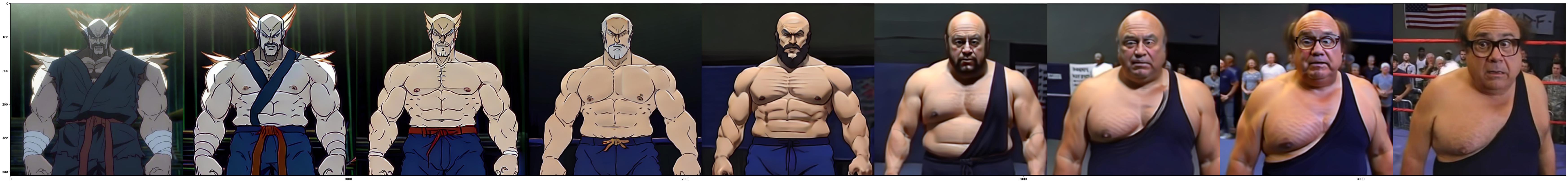
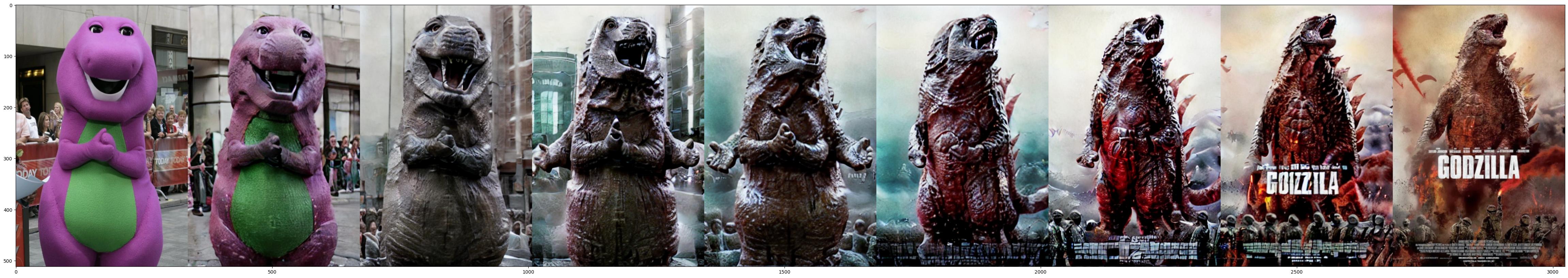
Figure 15: Additional morphing results with 9 frames.

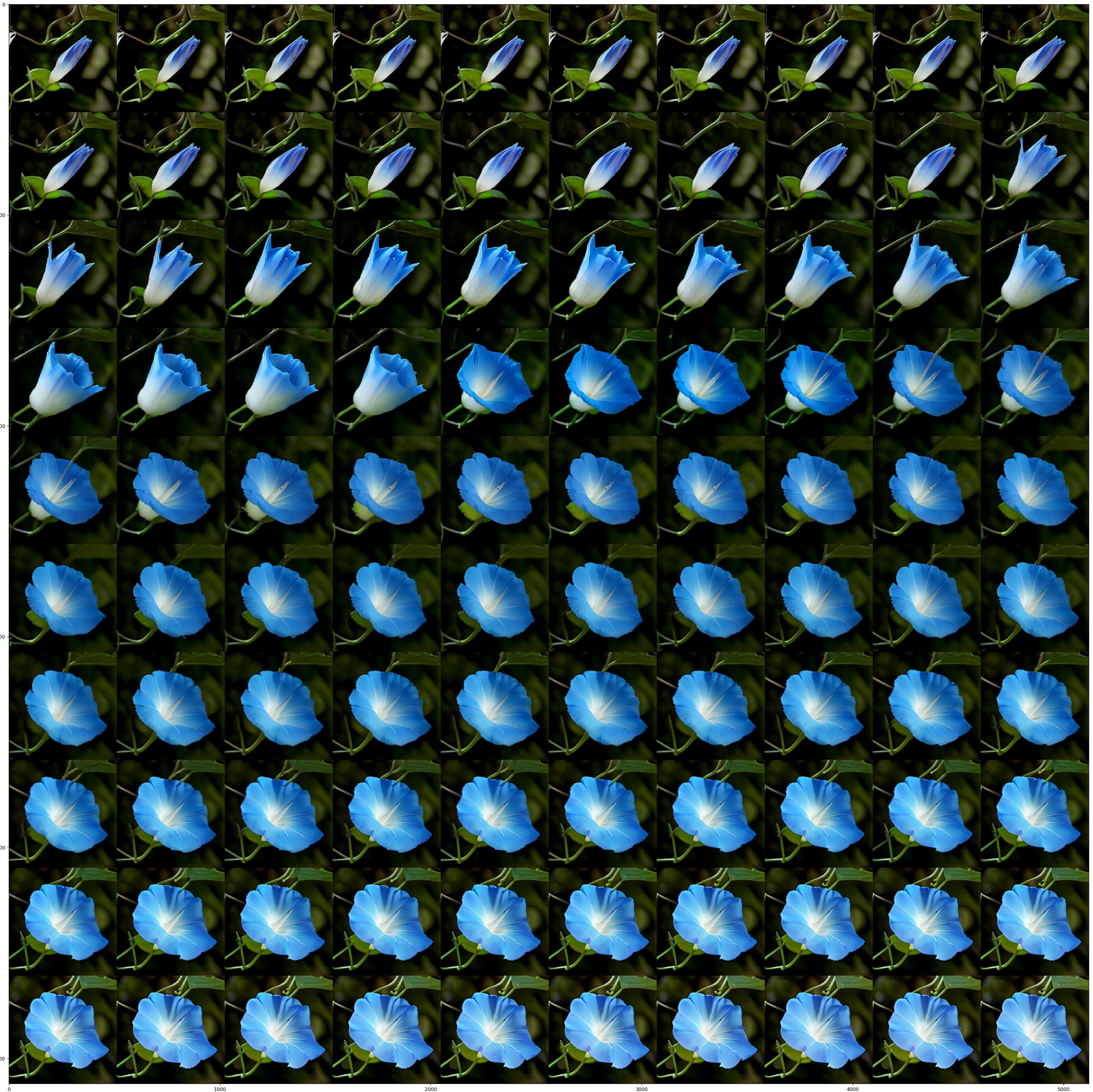
Figure 16: 100 interpolated images of “flower”.

A.6 Additional Morphing Results

Longer trajectory Morphing Results

To better illustrate the smoothness of morphing with our proposed IMPUS, we illustrate examples of 9 interpolated images in Fig. 15. We also illustrate 100 interpolated images using our uniform sampling in Fig. 16

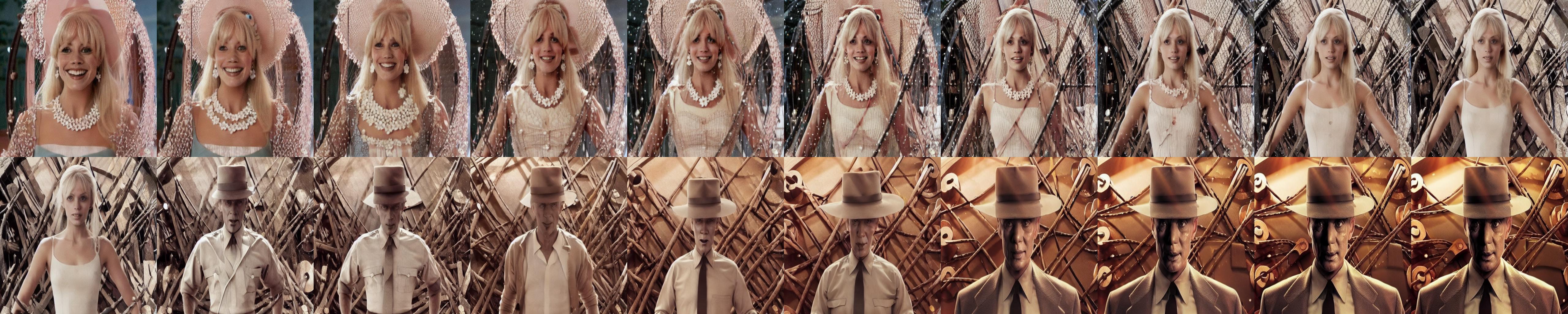
Figure 17: Morphing of Barbie and Oppenheimer.

Appendix B Image Attribution

• 25 pairs of images: https://github.com/clintonjwang/ControlNet

• Flower: https://www.youtube.com/watch?v=-sOdrJ6pusA

• Beetle:https://lancasteronline.com/features/home_garden/antiques-market-vintage-beetle-is-your-chance-to-relive-the-60s/article_308b7156-6713-11e7-95ed-732b1e8d88de.html

• Car: https://thebugagenda.com/green-iridescent-beetles/

• Camel:https://www.balisafarimarinepark.com/what-makes-camel-became-a-unique-animal/

• Lion:https://www.sfzoo.org/african-lion/

• Movie clip of Jurassic World: https://www.imdb.com/title/tt4881806/

• Running dog: https://youtu.be/_caOk6lycb0?si=g5o_j27IWcQWSKQp

• Movie poster from Barbie: https://www.imdb.com/title/tt1517268/

• Movie poster from Oppenheimer:https://www.imdb.com/title/tt15398776/

References

- Agueh & Carlier (2011) Martial Agueh and Guillaume Carlier. Barycenters in the wasserstein space. SIAM Journal on Mathematical Analysis, 43(2):904–924, 2011.
- Arad et al. (1994) Nur Arad, Nira Dyn, Daniel Reisfeld, and Yehezkel Yeshurun. Image warping by radial basis functions: Application to facial expressions. CVGIP: Graphical models and image processing, 56(2):161–172, 1994.
- Avrahami et al. (2023a) Omri Avrahami, Ohad Fried, and Dani Lischinski. Blended latent diffusion. ACM Trans. Graph., 42(4), jul 2023a. ISSN 0730-0301. doi: 10.1145/3592450. URL https://doi.org/10.1145/3592450.
- Avrahami et al. (2023b) Omri Avrahami, Thomas Hayes, Oran Gafni, Sonal Gupta, Yaniv Taigman, Devi Parikh, Dani Lischinski, Ohad Fried, and Xi Yin. Spatext: Spatio-textual representation for controllable image generation. In IEEE Conference on Computer Vision and Pattern Recognition (CVPR), pp. 18370–18380, 2023b.
- Balaji et al. (2022) Yogesh Balaji, Seungjun Nah, Xun Huang, Arash Vahdat, Jiaming Song, Karsten Kreis, Miika Aittala, Timo Aila, Samuli Laine, Bryan Catanzaro, et al. ediffi: Text-to-image diffusion models with an ensemble of expert denoisers. arXiv preprint arXiv:2211.01324, 2022.
- Bar-Tal et al. (2023) Omer Bar-Tal, Lior Yariv, Yaron Lipman, and Tali Dekel. Multidiffusion: Fusing diffusion paths for controlled image generation, 2023.
- Bayona (2018) Bayona. Jurassic world: Fallen kingdom. Film, 2018. URL https://www.imdb.com/title/tt4881806/. Directed by J.A. Bayona. Produced by Frank Marshall and Patrick Crowley. Universal Pictures.
- Brooks et al. (2023) Tim Brooks, Aleksander Holynski, and Alexei A. Efros. Instructpix2pix: Learning to follow image editing instructions. In IEEE Conference on Computer Vision and Pattern Recognition (CVPR), pp. 18392–18402, 2023.
- Brown et al. (2020) Tom Brown, Benjamin Mann, Nick Ryder, Melanie Subbiah, Jared D Kaplan, Prafulla Dhariwal, Arvind Neelakantan, Pranav Shyam, Girish Sastry, Amanda Askell, et al. Language models are few-shot learners. In Advances in Neural Information Processing Systems (NeurIPS), volume 33, pp. 1877–1901, 2020.
- Cheng et al. (2023) Bin Cheng, Zuhao Liu, Yunbo Peng, and Yue Lin. General image-to-image translation with one-shot image guidance. arXiv preprint arXiv:2307.14352, 2023.
- Chewi et al. (2020) Sinho Chewi, Tyler Maunu, Philippe Rigollet, and Austin J Stromme. Gradient descent algorithms for bures-wasserstein barycenters. In Conference on Learning Theory, pp. 1276–1304. PMLR, 2020.
- Cho et al. (2023) Wonwoong Cho, Hareesh Ravi, Midhun Harikumar, Vinh Khuc, Krishna Kumar Singh, Jingwan Lu, David I Inouye, and Ajinkya Kale. Towards enhanced controllability of diffusion models. arXiv preprint arXiv:2302.14368, 2023.
- Choi et al. (2023) Jooyoung Choi, Yunjey Choi, Yunji Kim, Junho Kim, and Sungroh Yoon. Custom-edit: Text-guided image editing with customized diffusion models. arXiv preprint arXiv:2305.15779, 2023.
- Choi et al. (2020) Yunjey Choi, Youngjung Uh, Jaejun Yoo, and Jung-Woo Ha. Stargan v2: Diverse image synthesis for multiple domains. In IEEE Conference on Computer Vision and Pattern Recognition (CVPR), pp. 8188–8197, 2020.
- Chowdhery et al. (2022) Aakanksha Chowdhery, Sharan Narang, Jacob Devlin, Maarten Bosma, Gaurav Mishra, Adam Roberts, Paul Barham, Hyung Won Chung, Charles Sutton, Sebastian Gehrmann, et al. Palm: Scaling language modeling with pathways. arXiv preprint arXiv:2204.02311, 2022.
- Daras & Dimakis (2022) Giannis Daras and Alexandros G Dimakis. Multiresolution textual inversion. arXiv preprint arXiv:2211.17115, 2022.
- Dhariwal & Nichol (2021) Prafulla Dhariwal and Alexander Nichol. Diffusion models beat GANs on image synthesis. In Advances in Neural Information Processing Systems (NeurIPS), pp. 8780–8794, 2021.
- Dong et al. (2023) Wenkai Dong, Song Xue, Xiaoyue Duan, and Shumin Han. Prompt tuning inversion for text-driven image editing using diffusion models. arXiv preprint arXiv:2305.04441, 2023.
- Dowd (2022) David Dowd. Python image morpher (pim). https://github.com/ddowd97/Python-Image-Morpher, 2022.
- EpicSlowMotionDog (2013) EpicSlowMotionDog. Dog running in epic slow motion 2 [hd]. Online video, 2013. URL https://youtu.be/_caOk6lycb0.
- Epstein et al. (2023) Dave Epstein, Allan Jabri, Ben Poole, Alexei A Efros, and Aleksander Holynski. Diffusion self-guidance for controllable image generation. arXiv preprint arXiv:2306.00986, 2023.
- Fei et al. (2023) Zhengcong Fei, Mingyuan Fan, and Junshi Huang. Gradient-free textual inversion. arXiv preprint arXiv:2304.05818, 2023.
- Fish et al. (2020) Noa Fish, Richard Zhang, Lilach Perry, Daniel Cohen-Or, Eli Shechtman, and Connelly Barnes. Image morphing with perceptual constraints and stn alignment. In Computer Graphics Forum, pp. 303–313. Wiley Online Library, 2020.
- Gal et al. (2022) Rinon Gal, Yuval Alaluf, Yuval Atzmon, Or Patashnik, Amit H Bermano, Gal Chechik, and Daniel Cohen-Or. An image is worth one word: Personalizing text-to-image generation using textual inversion. arXiv preprint arXiv:2208.01618, 2022.
- Goodfellow et al. (2014) Ian Goodfellow, Jean Pouget-Abadie, Mehdi Mirza, Bing Xu, David Warde-Farley, Sherjil Ozair, Aaron Courville, and Yoshua Bengio. Generative adversarial nets. In Advances in Neural Information Processing Systems (NeurIPS), 2014.
- Han et al. (2023) Ligong Han, Song Wen, Qi Chen, Zhixing Zhang, Kunpeng Song, Mengwei Ren, Ruijiang Gao, Yuxiao Chen, Di Liu 0003, Qilong Zhangli, et al. Improving tuning-free real image editing with proximal guidance. CoRR, 2023.
- Hertz et al. (2023) Amir Hertz, Ron Mokady, Jay Tenenbaum, Kfir Aberman, Yael Pritch, and Daniel Cohen-Or. Prompt-to-prompt image editing with cross-attention control. In International Conference on Learning Representations (ICLR), 2023.
- Heusel et al. (2017) Martin Heusel, Hubert Ramsauer, Thomas Unterthiner, Bernhard Nessler, and Sepp Hochreiter. Gans trained by a two time-scale update rule converge to a local nash equilibrium. In Advances in Neural Information Processing Systems (NeurIPS), 2017.
- Ho & Salimans (2022) Jonathan Ho and Tim Salimans. Classifier-free diffusion guidance. CoRR, abs/2207.12598, 2022. doi: 10.48550/arXiv.2207.12598. URL https://doi.org/10.48550/arXiv.2207.12598.
- Ho et al. (2020) Jonathan Ho, Ajay Jain, and Pieter Abbeel. Denoising diffusion probabilistic models. In Advances in Neural Information Processing Systems (NeurIPS), volume 33, pp. 6840–6851, 2020.
- Hu et al. (2021) Edward J Hu, Yelong Shen, Phillip Wallis, Zeyuan Allen-Zhu, Yuanzhi Li, Shean Wang, Lu Wang, and Weizhu Chen. Lora: Low-rank adaptation of large language models. arXiv preprint arXiv:2106.09685, 2021.
- Huberman-Spiegelglas et al. (2023) Inbar Huberman-Spiegelglas, Vladimir Kulikov, and Tomer Michaeli. An edit friendly ddpm noise space: Inversion and manipulations. arXiv preprint arXiv:2304.06140, 2023.
- Karras et al. (2017) Tero Karras, Timo Aila, Samuli Laine, and Jaakko Lehtinen. Progressive growing of gans for improved quality, stability, and variation. arXiv preprint arXiv:1710.10196, 2017.
- Karras et al. (2019) Tero Karras, Samuli Laine, and Timo Aila. A style-based generator architecture for generative adversarial networks. In IEEE Conference on Computer Vision and Pattern Recognition (CVPR), pp. 4401–4410, 2019.
- Karras et al. (2022) Tero Karras, Miika Aittala, Timo Aila, and Samuli Laine. Elucidating the design space of diffusion-based generative models. Advances in Neural Information Processing Systems, 35:26565–26577, 2022.
- Kawar et al. (2023) Bahjat Kawar, Shiran Zada, Oran Lang, Omer Tov, Huiwen Chang, Tali Dekel, Inbar Mosseri, and Michal Irani. Imagic: Text-based real image editing with diffusion models. In IEEE Conference on Computer Vision and Pattern Recognition (CVPR), pp. 6007–6017, 2023.
- Khrulkov et al. (2022) Valentin Khrulkov, Gleb Ryzhakov, Andrei Chertkov, and Ivan Oseledets. Understanding ddpm latent codes through optimal transport. In International Conference on Learning Representations (ICLR), 2022.
- Kim et al. (2023) Beomsu Kim, Gihyun Kwon, Kwanyoung Kim, and Jong Chul Ye. Unpaired image-to-image translation via neural schrödinger bridge. arXiv preprint arXiv:2305.15086, 2023.
- Kim et al. (2022) Gwanghyun Kim, Taesung Kwon, and Jong Chul Ye. Diffusionclip: Text-guided diffusion models for robust image manipulation. In IEEE Conference on Computer Vision and Pattern Recognition (CVPR), pp. 2426–2435, 2022.
- Kingma & Ba (2014) Diederik P Kingma and Jimmy Ba. Adam: A method for stochastic optimization. arXiv preprint arXiv:1412.6980, 2014.
- Kwon et al. (2023) Mingi Kwon, Jaeseok Jeong, and Youngjung Uh. Diffusion models already have a semantic latent space. In The Eleventh International Conference on Learning Representations, 2023. URL https://openreview.net/forum?id=pd1P2eUBVfq.
- Lee et al. (1995) Seungyong Lee, Kyungyong Chwa, and Sungyong Shin. Image metamorphosis using snakes and free-form deformations. In Proceedings of the 22nd annual conference on Computer graphics and interactive techniques, pp. 439–448, 1995.
- Lee et al. (1996) Seungyong Lee, George Wolberg, Kyung Yong Chwa, and Sung Yong Shin. Image metamorphosis with scattered feature constraints. IEEE Trans. Vis. Comput. Graph., 2(4):337–354, 1996.
- Li et al. (2023a) Pengzhi Li, Qinxuan Huang, Yikang Ding, and Zhiheng Li. Layerdiffusion: Layered controlled image editing with diffusion models. arXiv preprint arXiv:2305.18676, 2023a.
- Li et al. (2023b) Senmao Li, Joost van de Weijer, Taihang Hu, Fahad Shahbaz Khan, Qibin Hou, Yaxing Wang, and Jian Yang. Stylediffusion: Prompt-embedding inversion for text-based editing. arXiv preprint arXiv:2303.15649, 2023b.
- Liang et al. (2023) Feng Liang, Bichen Wu, Xiaoliang Dai, Kunpeng Li, Yinan Zhao, Hang Zhang, Peizhao Zhang, Peter Vajda, and Diana Marculescu. Open-vocabulary semantic segmentation with mask-adapted clip. In IEEE Conference on Computer Vision and Pattern Recognition (CVPR), pp. 7061–7070, 2023.
- Liang et al. (2022) Weixin Liang, Yuhui Zhang, Yongchan Kwon, Serena Yeung, and James Y. Zou. Mind the gap: Understanding the modality gap in multi-modal contrastive representation learning. In Advances in Neural Information Processing Systems (NeurIPS), 2022.
- Liao et al. (2014) Jing Liao, Rodolfo S. Lima, Diego Nehab, Hugues Hoppe, Pedro V. Sander, and Jinhui Yu. Automating image morphing using structural similarity on a halfway domain. ACM Trans. Graph., 33(5):168:1–168:12, 2014.
- Liu & Liu (2023) Chang Liu and Dong Liu. Late-constraint diffusion guidance for controllable image synthesis. arXiv preprint arXiv:2305.11520, 2023.
- Liu et al. (2022) Luping Liu, Yi Ren, Zhijie Lin, and Zhou Zhao. Pseudo numerical methods for diffusion models on manifolds. arXiv preprint arXiv:2202.09778, 2022.
- Loshchilov & Hutter (2018) Ilya Loshchilov and Frank Hutter. Decoupled weight decay regularization. In International Conference on Learning Representations, 2018.
- Lu et al. (2022a) Cheng Lu, Yuhao Zhou, Fan Bao, Jianfei Chen, Chongxuan Li, and Jun Zhu. Dpm-solver: A fast ode solver for diffusion probabilistic model sampling in around 10 steps. In Advances in Neural Information Processing Systems (NeurIPS), pp. 5775–5787, 2022a.
- Lu et al. (2022b) Cheng Lu, Yuhao Zhou, Fan Bao, Jianfei Chen, Chongxuan Li, and Jun Zhu. Dpm-solver++: Fast solver for guided sampling of diffusion probabilistic models. arXiv preprint arXiv:2211.01095, 2022b.
- Lugmayr et al. (2022) Andreas Lugmayr, Martin Danelljan, Andres Romero, Fisher Yu, Radu Timofte, and Luc Van Gool. Repaint: Inpainting using denoising diffusion probabilistic models. In IEEE Conference on Computer Vision and Pattern Recognition (CVPR), pp. 11461–11471, 2022.
- Lunarring (2022) Lunarring. Latent blending. https://github.com/lunarring/latentblending, 2022.
- Meng et al. (2021) Chenlin Meng, Yutong He, Yang Song, Jiaming Song, Jiajun Wu, Jun-Yan Zhu, and Stefano Ermon. Sdedit: Guided image synthesis and editing with stochastic differential equations. arXiv preprint arXiv:2108.01073, 2021.
- Miller & Younes (2001) Michael I. Miller and Laurent Younes. Group actions, homeomorphisms, and matching: A general framework. International Journal of Computer Vision, 41:61–84, 2001.
- Mokady et al. (2023) Ron Mokady, Amir Hertz, Kfir Aberman, Yael Pritch, and Daniel Cohen-Or. Null-text inversion for editing real images using guided diffusion models. In IEEE Conference on Computer Vision and Pattern Recognition (CVPR), pp. 6038–6047, 2023.
- Nichol et al. (2022) Alexander Quinn Nichol, Prafulla Dhariwal, Aditya Ramesh, Pranav Shyam, Pamela Mishkin, Bob McGrew, Ilya Sutskever, and Mark Chen. GLIDE: towards photorealistic image generation and editing with text-guided diffusion models. In International Conference on Machine Learning (ICML), pp. 16784–16804, 2022.
- Nri (2022) Chigozie Nri. Differentiable morphing. https://github.com/volotat/DiffMorph, 2022.
- Parmar et al. (2023) Gaurav Parmar, Krishna Kumar Singh, Richard Zhang, Yijun Li, Jingwan Lu, and Jun-Yan Zhu. Zero-shot image-to-image translation. arXiv preprint arXiv:2302.03027, 2023.
- Pérez et al. (2023) Patrick Pérez, Michel Gangnet, and Andrew Blake. Poisson image editing. In Seminal Graphics Papers: Pushing the Boundaries, Volume 2, pp. 577–582, 2023.
- Preechakul et al. (2022) Konpat Preechakul, Nattanat Chatthee, Suttisak Wizadwongsa, and Supasorn Suwajanakorn. Diffusion autoencoders: Toward a meaningful and decodable representation. In IEEE Conference on Computer Vision and Pattern Recognition (CVPR), pp. 10619–10629, 2022.
- Radford et al. (2021) Alec Radford, Jong Wook Kim, Chris Hallacy, Aditya Ramesh, Gabriel Goh, Sandhini Agarwal, Girish Sastry, Amanda Askell, Pamela Mishkin, Jack Clark, et al. Learning transferable visual models from natural language supervision. In International Conference on Machine Learning (ICML), pp. 8748–8763. PMLR, 2021.
- Rajković (2023) Marko Rajković. Geodesics, Splines, and Embeddings in Spaces of Images. PhD thesis, Universitäts-und Landesbibliothek Bonn, 2023.
- Ramesh et al. (2022) Aditya Ramesh, Prafulla Dhariwal, Alex Nichol, Casey Chu, and Mark Chen. Hierarchical text-conditional image generation with clip latents. arXiv preprint arXiv:2204.06125, 1(2):3, 2022.
- Rombach et al. (2022) Robin Rombach, Andreas Blattmann, Dominik Lorenz, Patrick Esser, and Björn Ommer. High-resolution image synthesis with latent diffusion models. In IEEE Conference on Computer Vision and Pattern Recognition (CVPR), pp. 10684–10695, 2022.
- Saharia et al. (2022) Chitwan Saharia, William Chan, Saurabh Saxena, Lala Li, Jay Whang, Emily L Denton, Kamyar Ghasemipour, Raphael Gontijo Lopes, Burcu Karagol Ayan, Tim Salimans, et al. Photorealistic text-to-image diffusion models with deep language understanding. In Advances in Neural Information Processing Systems (NeurIPS), pp. 36479–36494, 2022.
- Seitz & Dyer (1996) Steven M Seitz and Charles R Dyer. View morphing. In Proceedings of the 23rd annual conference on Computer graphics and interactive techniques, pp. 21–30, 1996.
- Selvaraju et al. (2017) Ramprasaath R Selvaraju, Michael Cogswell, Abhishek Das, Ramakrishna Vedantam, Devi Parikh, and Dhruv Batra. Grad-cam: Visual explanations from deep networks via gradient-based localization. In IEEE International Conference on Computer Vision (ICCV), pp. 618–626, 2017.
- Shechtman et al. (2010) Eli Shechtman, Alex Rav-Acha, Michal Irani, and Steve Seitz. Regenerative morphing. In IEEE Conference on Computer Vision and Pattern Recognition (CVPR), pp. 615–622. IEEE, 2010.
- Simon & Aberdam (2020) Dror Simon and Aviad Aberdam. Barycenters of natural images constrained wasserstein barycenters for image morphing. In IEEE Conference on Computer Vision and Pattern Recognition (CVPR), pp. 7910–7919, 2020.
- Song et al. (2020a) Jiaming Song, Chenlin Meng, and Stefano Ermon. Denoising diffusion implicit models. arXiv preprint arXiv:2010.02502, 2020a.
- Song et al. (2020b) Yang Song, Jascha Sohl-Dickstein, Diederik P Kingma, Abhishek Kumar, Stefano Ermon, and Ben Poole. Score-based generative modeling through stochastic differential equations. arXiv preprint arXiv:2011.13456, 2020b.
- Su et al. (2023) Xuan Su, Jiaming Song, Chenlin Meng, and Stefano Ermon. Dual diffusion implicit bridges for image-to-image translation. In iclr, 2023.
- Touvron et al. (2023) Hugo Touvron, Thibaut Lavril, Gautier Izacard, Xavier Martinet, Marie-Anne Lachaux, Timothée Lacroix, Baptiste Rozière, Naman Goyal, Eric Hambro, Faisal Azhar, et al. Llama: Open and efficient foundation language models. arXiv preprint arXiv:2302.13971, 2023.
- Tsaban & Passos (2023) Linoy Tsaban and Apolinário Passos. Ledits: Real image editing with ddpm inversion and semantic guidance. arXiv preprint arXiv:2307.00522, 2023.
- Tumanyan et al. (2023) Narek Tumanyan, Michal Geyer, Shai Bagon, and Tali Dekel. Plug-and-play diffusion features for text-driven image-to-image translation. In IEEE Conference on Computer Vision and Pattern Recognition (CVPR), pp. 1921–1930, 2023.
- Villani (2016) C. Villani. Optimal Transport: Old and New. Grundlehren der mathematischen Wissenschaften. Springer Berlin Heidelberg, 2016. ISBN 9783662501801. URL https://books.google.com.au/books?id=5p8SDAEACAAJ.
- Villani (2021) Cédric Villani. Topics in optimal transportation, volume 58. American Mathematical Soc., 2021.
- Voynov et al. (2023) Andrey Voynov, Qinghao Chu, Daniel Cohen-Or, and Kfir Aberman. : Extended textual conditioning in text-to-image generation. arXiv preprint arXiv:2303.09522, 2023.
- Wallace et al. (2023) Bram Wallace, Akash Gokul, and Nikhil Naik. Edict: Exact diffusion inversion via coupled transformations. In IEEE Conference on Computer Vision and Pattern Recognition (CVPR), pp. 22532–22541, 2023.
- Wang & Golland (2023) Clinton J. Wang and Polina Golland. Interpolating between images with diffusion models. CoRR, abs/2307.12560, 2023. doi: 10.48550/arXiv.2307.12560. URL https://doi.org/10.48550/arXiv.2307.12560.
- Wang et al. (2023a) Qian Wang, Biao Zhang, Michael Birsak, and Peter Wonka. Mdp: A generalized framework for text-guided image editing by manipulating the diffusion path. arXiv preprint arXiv:2303.16765, 2023a.
- Wang et al. (2023b) Zhengyi Wang, Cheng Lu, Yikai Wang, Fan Bao, Chongxuan Li, Hang Su, and Jun Zhu. Prolificdreamer: High-fidelity and diverse text-to-3d generation with variational score distillation. arXiv preprint arXiv:2305.16213, 2023b.
- Wei et al. (2023) Yuxiang Wei, Yabo Zhang, Zhilong Ji, Jinfeng Bai, Lei Zhang, and Wangmeng Zuo. Elite: Encoding visual concepts into textual embeddings for customized text-to-image generation. In IEEE International Conference on Computer Vision (ICCV), 2023.
- Wolberg (1998) George Wolberg. Image morphing: a survey. The visual computer, 14(8-9):360–372, 1998.
- Wu & la Torre (2022) Chen Henry Wu and Fernando De la Torre. Making text-to-image diffusion models zero-shot image-to-image editors by inferring ”random seeds”. In NeurIPS 2022 Workshop on Score-Based Methods, 2022. URL https://openreview.net/forum?id=NneX9CkWvB.
- Xu et al. (2023) Mengde Xu, Zheng Zhang, Fangyun Wei, Han Hu, and Xiang Bai. Side adapter network for open-vocabulary semantic segmentation. In IEEE Conference on Computer Vision and Pattern Recognition (CVPR), pp. 2945–2954, 2023.
- Yang et al. (2023a) Binxin Yang, Shuyang Gu, Bo Zhang, Ting Zhang, Xuejin Chen, Xiaoyan Sun, Dong Chen, and Fang Wen. Paint by example: Exemplar-based image editing with diffusion models. In IEEE Conference on Computer Vision and Pattern Recognition (CVPR), pp. 18381–18391, 2023a.
- Yang et al. (2023b) Yue Yang, Kaipeng Zhang, Yuying Ge, Wenqi Shao, Zeyue Xue, Yu Qiao, and Ping Luo. Align, adapt and inject: Sound-guided unified image generation. arXiv preprint arXiv:2306.11504, 2023b.
- Yu et al. (2015) Fisher Yu, Ari Seff, Yinda Zhang, Shuran Song, Thomas Funkhouser, and Jianxiong Xiao. Lsun: Construction of a large-scale image dataset using deep learning with humans in the loop. arXiv preprint arXiv:1506.03365, 2015.
- Zhang et al. (2023a) Guoqiang Zhang, Jonathan P Lewis, and W Bastiaan Kleijn. Exact diffusion inversion via bi-directional integration approximation. arXiv preprint arXiv:2307.10829, 2023a.
- Zhang et al. (2023b) Jiaxin Zhang, Kamalika Das, and Sricharan Kumar. On the robustness of diffusion inversion in image manipulation. In ICLR 2023 Workshop on Trustworthy and Reliable Large-Scale Machine Learning Models, 2023b. URL https://openreview.net/forum?id=fr8kurMWJIP.
- Zhang et al. (2020) Lingzhi Zhang, Tarmily Wen, and Jianbo Shi. Deep image blending. In IEEE Winter Conference on Applications of Computer Vision (WACV), pp. 231–240, 2020.
- Zhang & Agrawala (2023) Lvmin Zhang and Maneesh Agrawala. Adding conditional control to text-to-image diffusion models. arXiv preprint arXiv:2302.05543, 2023.
- Zhang et al. (2018) Richard Zhang, Phillip Isola, Alexei A Efros, Eli Shechtman, and Oliver Wang. The unreasonable effectiveness of deep features as a perceptual metric. In IEEE Conference on Computer Vision and Pattern Recognition (CVPR), pp. 586–595, 2018.
- Zhang et al. (2023c) Zhixing Zhang, Ligong Han, Arnab Ghosh, Dimitris N Metaxas, and Jian Ren. Sine: Single image editing with text-to-image diffusion models. In IEEE Conference on Computer Vision and Pattern Recognition (CVPR), pp. 6027–6037, 2023c.
- Zhang et al. (2023d) Zhongping Zhang, Jian Zheng, Jacob Zhiyuan Fang, and Bryan A Plummer. Text-to-image editing by image information removal. arXiv preprint arXiv:2305.17489, 2023d.
- Zhu et al. (2007) Lei Zhu, Yan Yang, Steven Haker, and Allen Tannenbaum. An image morphing technique based on optimal mass preserving mapping. IEEE Transactions on Image Processing (TIP), 16(6):1481–1495, 2007.
- Zope & Zope (2017) Bhushan Zope and Soniya B Zope. A survey of morphing techniques. International Journal of Advanced Engineering, Management and Science, 3(2):239773, 2017.