Real-Time Probabilistic Programming

Abstract

Complex cyber-physical systems interact in real-time and must consider both timing and uncertainty. Developing software for such systems is both expensive and difficult, especially when modeling, inference, and real-time behavior need to be developed from scratch. Recently, a new kind of language has emerged—called probabilistic programming languages (PPLs)—that simplify modeling and inference by separating the concerns between probabilistic modeling and inference algorithm implementation. However, these languages have primarily been designed for offline problems, not online real-time systems. In this paper, we combine PPLs and real-time programming primitives by introducing the concept of real-time probabilistic programming languages (RTPPL). We develop an RTPPL called ProbTime and demonstrate its usability on an automotive testbed performing indoor positioning and braking. Moreover, we study fundamental properties and design alternatives for runtime behavior, including a new fairness-guided approach that automatically optimizes the accuracy of a ProbTime system under schedulability constraints.

I Introduction

Probabilistic programming [1, 2] is an emerging programming paradigm that enables simple and expressive probabilistic modeling of complex systems. Specifically, the key motivation for probabilistic programming languages (PPLs) is to separate the concerns between the model (the probabilistic program) and the inference algorithm. Such separation enables the system designer to focus on the modeling problem without the need to have deep knowledge of Bayesian inference algorithms, such as Sequential Monte Carlo (SMC) [3, 4] or Markov chain Monte Carlo (MCMC) [5] methods.

There exist many research PPLs, including Pyro [6], WebPPL [7], Stan [8], Anglican [9], Turing [10], Gen [11], and Miking CorePPL [12]. These PPLs focus on offline inference problems, such as data cleaning [13], phylogenetics [14], computer vision [15], or cognitive science [16], where time and timing properties are not explicitly part of the programming model. Likewise, many languages and environments exist for programming real-time systems [17, 18, 19] with no built-in support for probabilistic modeling and inference. Although some recent work exists on using probabilistic programming for reactive synchronous systems [20, 21] and for continuous time systems [22], no existing work combines probabilistic programming with real-time programming, where both inference and timing constructs are first-class.

Combining probabilistic programming with real-time programming results in several significant research challenges. Specifically, we identify two key challenges: (i) how to incorporate language constructs for both timing and probabilistic reasoning in a sound manner, and (ii) how to design and implement efficient compiler and runtime systems that meet both real-time constraints and inference accuracy requirements.

In this paper, we introduce a new kind of language that we call real-time probabilistic programming languages (RTPPLs). In this paradigm, users can focus on the modeling aspect of inferring unknown parameters of a real-time system without the need to know details of how timing aspects or inference algorithms are implemented. We motivate the ideas behind this new kind of language and outline the main design challenges. To demonstrate the concepts of RTPPL, we develop the first RTPPL called ProbTime, which includes probabilistic programming primitives, timing primitives, and primitives for designing modular task-based real-time systems. We create a compiler toolchain for ProbTime and demonstrate how it can be efficiently implemented in a real case study for automotive positioning and braking. Key aspects of our design include efficient real-time inference using Sequential Monte-Carlo (SMC) inference and the use of timing programming points inspired by Timed C [17]. We have implemented the overall compiler within the Miking framework [23] as part of the Miking CorePPL effort [12].

⬇

1var coinFlip = function() {

2 var x = sample(Beta({a:2, b:2}))

3 observe(Bernoulli({p:x}), true)

4 ...

5 return x

6}

(a) Line 2 defines the latent variable x and gives the prior Beta(2,2). Line 3 shows an observation statement (observing a true value), and line 5 states that the posterior for x should be computed.

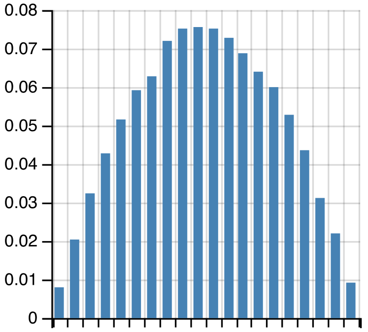
(b) Prior distribution Beta(2,2) for latent variable x.

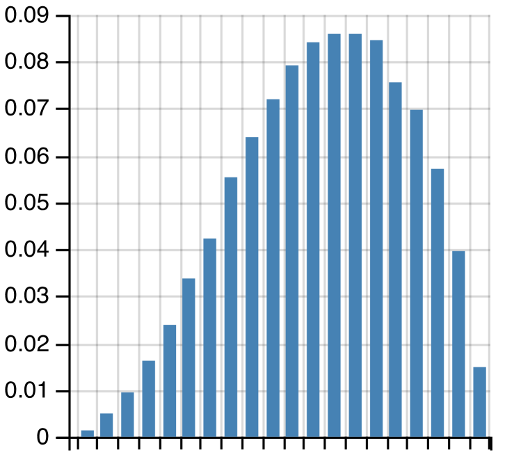
(c) Posterior distribution for x, one true observation.

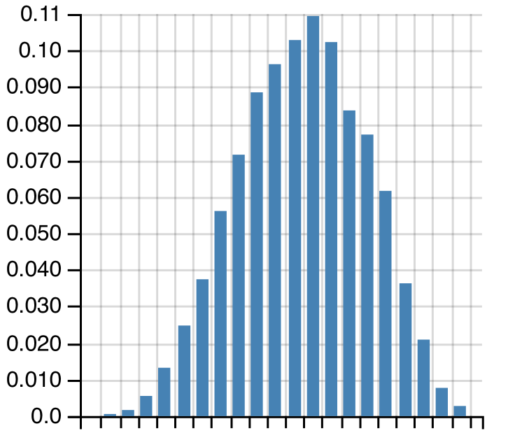
(d) Posterior distri-bution, observations [T, F, F, T, T]

Figure 1: A simple WebPPL program modeling a coin flip. Fig. (1(a)) shows the source code and Fig. (1(b)) the prior distribution. Fig. (1(c)) gives the posterior distribution after one coin flip, and Fig. (1(d)) the posterior after a sequence of 5 coin flips.

In summary, we make the following contributions:

• We introduce the new paradigm of real-time probabilistic programming (RTPPL), motivate why it is essential, and outline major design challenges (Section II).

• We design and implement ProbTime, the first domain-specific language within the domain of RTPPL (Section III).

• We present a novel automated offline configuration approach that maximizes inference accuracy under real-time constraints. Specifically, we introduce the concepts of particle and execution-time fairness within the context of real-time probabilistic programming (Section IV) and study how they can be incorporated in an automated configuration setting (Section V).

• We develop an automotive testbed including both hardware and software. As part of our case study, we demonstrate how a non-trivial ProbTime program can perform indoor positioning and braking in a real-time physical environment (Section VI).

II Motivation and Challenges with RTPPL

This section introduces the main ideas of probabilistic programming, motivates why it is useful for real-time systems, and outlines some of the key challenges.

II-A Probabilistic Programming Languages (PPLs)

Probabilistic programming is a rather recent programming paradigm that enables probabilistic modeling where the models can be described as Turing complete programs. Specifically, given a probabilistic program $f$, observed data, and prior knowledge about the distribution of latent variables $\theta$, a PPL execution environment can automatically approximate the posterior distribution of $\theta$. Recall Bayes’ rule

$$p(\theta,\textbf{data})=\frac{p(\textbf{data},\theta)p(\theta)}{p(\textbf{data})}$$ (1)

where $p(\theta,\textbf{data})$ is the posterior, $p(\textbf{data},\theta)$ the likelihood, $p(\theta)$ the prior, and $p(\textbf{data})$ the normalizing constant. Using a simple toy probabilistic program, we will now explain how standard PPL constructs relate to Bayes’ rule.

Consider Fig. 1(a), which is written in WebPPL [7], a PPL designed at Stanford that is especially suitable for teaching. We use this simple coin-flip example to give an intuition for the fundamental constructs in a PPL. The model is defined as a function that defines one random variable x (line 2) using the sample construct. In this example, random variable x models the probability that a coin flip becomes true (we assume that true means heads and false means tails). For instance, if $p(\texttt{x})=0.5$, the coin is fair, whereas if, e.g., $p(\texttt{x})=0.7$, it is unfair and more likely to result in true when flipped.

The sample construct on line 2 both defines the random variable and gives its prior, in this case, the Beta distribution with parameters a and b equal to $2$. If we sample from this prior, we get the Beta distribution depicted in Fig. 1(b). Note how the sample constructs in a probabilistic program correspond to the prior $p(\theta)$ in Bayes’ rule (Equation 1).

However, the goal of Bayesian inference is to estimate the posterior for a latent variable, given some observations. Line 3 in the program shows an observe statement, where a coin flip of value true is observed according to the Bernoulli distribution. Note how the Bernoulli distribution’s parameter p depends on the random variable x. Consider Fig. 1(c), which depicts the inferred posterior distribution given one observed true coin flip. As expected, the distribution has shifted slightly to the right, meaning that given one sample, the coin is estimated to be somewhat biased towards resulting in true values. Note also how observe statements in a probabilistic program correspond to the likelihood $p(\textbf{data},\theta)$ in Bayes’ rule. That is, the likelihood we observe some specific data, given a certain latent variable $\theta$.

If we extend Fig. 1(a) with in total five observations [true, false, false, true, true] in a sequence (illustrated with ... on line 4), the resulting posterior looks like Fig. 1(d). We can note the following: (i) the resulting mean is still slightly towards true (we have observed one more true value), and (ii) the variance is lower (the peak is slightly thinner). The latter case is a direct consequence of Bayesian inference and one of its key benefits: given the prior and the observed data, the posterior correctly represents the uncertainty of the result, not just a point estimate.

The inference of the toy example can be inferred using many different inference strategies, such as sequential Monte Carlo (SMC) or Markov chain Monte Carlo (MCMC). In this work, we focus on SMC, and one of its instances, also known as the particle filter [24] algorithm, because of its strength in this kind of applications. The intuition of particle filters is that inference is done by forward executing the probabilistic program (the model) multiple times (potentially in parallel). Each such execution point is called a particle and consists at the end of a weight (how likely the particle is) and the output values, where the set of all particles forms the posterior distribution. Intuitively, the more particles, the better the accuracy of the approximate inference. There are many more details of the algorithm (e.g., resampling strategies) that are outside the scope of this paper, and an interested reader is referred to this technical overview by Naesseth et al. [25]. Although hiding the details of the inference algorithm is one of the key ideas of PPLs (separating the model from inference), the number of particles is essential for automatic inference and scheduling. Hence, this is a key concept in our work and will be discussed further in this paper.

II-B Real-Time Probabilistic Programming (RTPPL)

⬇

57system {

58 sensor speed1 : Float///\label{lst:model:sa1}

59 sensor speed2 : Float

60 actuator brake : Float///\label{lst:model:sa2}

61 task speedEst1 = Speed(250ms) importance 1///\label{lst:model:tasks1}

62 task speedEst2 = Speed(500ms) importance 1

63 task pos = Position(1s) importance 3

64 task braking = Brake(300ms) importance 4///\label{lst:model:tasks2}

65 speed1 -> speedEst1.in1///\label{lst:model:conn1}

66 speed2 -> speedEst2.in1

67 speedEst1.out -> pos.in1///\label{lst:model:s1conn1}

68 speedEst1.out -> braking.in1///\label{lst:model:s1conn2}

69 speedEst2.out -> pos.in2

70 speedEst2.out -> braking.in2

71 pos.out -> braking.in3

72 braking.out -> brake///\label{lst:model:conn2}

73}

(a) The system declaration of a ProbTime program.

(b) A graphical representation of the system defined in Fig. 2(a). The system consists of two sensors, speed1 and speed2 on the left-hand side, four tasks speedEst1, speedEst2, pos, and braking in the middle, and an actuator brake on the right-hand side. Lines represent connections, where the white box represents the output port and the incoming arrow represents the input port.

Figure 2: Example system of a ProbTime program in graphical and textual form.

The toy example of a coin flip in the previous example gives an intuition of probabilistic programming but does not show its power in large-scale applications. Probabilistic programming is today used in several domains, but surprisingly little has been done within the real-time context. Although a rich literature exists on using Bayesian inference and filtering algorithms (e.g., particle filters in aircraft positioning [24]), these algorithms are typically hand-coded where both the probabilistic model and the inference algorithm are combined. This means that a developer needs to have deep insights into three different fields: (i) probabilistic modeling, (ii) Bayesian inference algorithms, and (iii) real-time programming aspects. Standard probabilistic programming is motivated by the appealing argument of separating (i) and (ii), thus enabling probabilistic modeling by developers without deep knowledge of how to implement inference efficiently and correctly. However, so far, probabilistic programming has not been combined with (iii) real-time aspects, such as timing, scheduling, and worst-case execution time estimation. This paper aims to make the first step towards mitigating this gap. We call this approach real-time probabilistic programming (RTPPL).

How can an RTPPL be designed? For instance, we can extend an existing PPL with timing semantics, extend an existing real-time language with PPL constructs, or create a new domain-specific language (DSL) that includes only a minimal number of constructs for reasoning about timing and probabilistic inference. In this research work, we chose the latter to avoid accidental complexity when extending large existing languages. In particular, our purpose is to study the fundamentals of this new kind of language category. We identify and study the following key challenges with RTPPLs:

• Challenge A: In an RTPPL, how can we encode real-time properties (deadlines, periodicity, etc.) and probabilistic constructs (sampling, observations, etc.) without forcing the user to specify low-level details such as particle counts and worst-case execution times?

• Challenge B: How can a runtime environment be constructed, such that a fair amount of time is spent on different tasks, giving the right number of particles for each task (for accuracy), where the system is still known to be statically schedulable?

We address Challenge A in the following section (Section III) by designing a new minimalistic research DSL called ProbTime. Using the new DSL, we address Challenge B by studying two new concepts: particle fairness and execution-time fairness (Section IV), and how particle counts, execution-time measurements, and scheduling can be performed automatically to get a fair and working configuration (Section V).

III ProbTime - an RTPPL

In this section, we introduce a new real-time probabilistic programming language called ProbTime, a statically typed domain-specific language. We illustrate the timing and probabilistic constructs in the language using a small example, followed by a short overview of the compiler implementation.

III-A System Declaration

We present a ProbTime system declaration implementing automated braking for a train in Fig. 2. The system keeps track of the position of the train, using the automatic brakes before collision. The train provides observation data via two speed sensors with varying frequencies and accuracy (left side in Fig. 2(b)) and our system can activate its brakes via an actuator (right side in Fig. 2(b)). In Fig. 2(a), we first declare the sensors and actuators and associate them with a type, determining the type of data they operate on (lines LABEL:lst:model:sa1-LABEL:lst:model:sa2). The squares in the graphical representation represent the tasks of our system. We instantiate the tasks on lines LABEL:lst:model:tasks1-LABEL:lst:model:tasks2. Note that we can instantiate multiple tasks from the same template (in this case the Speed template). An important and unique construct in ProbTime is the importance construct that states the relative importance between tasks. In terms of fairness, lines  LABEL:lst:model:tasks1-LABEL:lst:model:tasks2 state that pos and braking should be allocated more execution time or run more particles compared to the speedEst1 and speedEst2 tasks. We discuss this further in Section IV.

On lines LABEL:lst:model:conn1-LABEL:lst:model:conn2 in Fig. 2(a), we declare the connections using arrow syntax a -> b, specifying that data written to the output port identified by a is delivered to the input port identified by b. We use the names of sensors and actuators as port identifiers, and we use x.y as an identifier for the port y of task x.

III-B Templates and Timing Constructs

Continuing with the train braking example, we outline the definitions of task templates Speed and Position in Listing 1. Consider the definition of the Speed template (lines LABEL:lst:model:speed1-LABEL:lst:model:speed2). We declare the input port in1 and the output port out on lines LABEL:lst:model:speedin1-LABEL:lst:model:speedout, and annotate them with types.

In Position, we use our prior belief of the train’s position when estimating its current position. However, variables in ProbTime are immutable by default. We apply update d to the while-loop on line LABEL:lst:model:pos-whileupd to indicate that we want updates to d to be visible in the next iteration of the loop and in the code following the loop. When we estimate the current speed of the train, we do not use our prior belief. Therefore, we omit the update in the while-loop on line LABEL:lst:model:speed-while.

Listing 1: Definition of the Speed and Position task templates.

⬇

24template Speed(period : Int) {///\label{lst:model:speed1}

25 input in1 : Float///\label{lst:model:speedin1}

26 output out : Dist(Float)///\label{lst:model:speedout}

27 while true {///\label{lst:model:speed-while}

28 delay period

29 read in1 to obs///\label{lst:model:speed-read}

30 infer speedModel(obs) to d///\label{lst:model:speed-infer}

31 write d to out///\label{lst:model:speed-write}

32 }

33}///\label{lst:model:speed2}

34template Position() {

35 input in1 : Dist(Float)

36 input in2 : Dist(Float)

37 output out : Dist(Float)

38 infer initPos() to d

39 while true update d {///\label{lst:model:pos-whileupd}

40 delay 1s///\label{lst:model:delay-fixed}

41 read in1 to speed1

42 read in2 to speed2

43 infer positionModel(d, speed1, speed2) to d

44 write d to out offset 500ms///\label{lst:model:pos-write}

45 }

46}

We control timing in ProbTime using the delay statement. Each delay represents a timing point and results in a relative delay to the previous timing point, where we consider the start of the program as the initial timing point. This concept is inspired by sdelays of Timed C [17]. However, a key difference is that our delay construct does not return the amount of overrun. Instead, our automated configuration adapts the execution times of tasks to ensure they remain schedulable (discussed in Section V). We denote the execution between two consecutive timing points as one task instance. Hence, a timing point represents the release of a new task instance. For instance, on line LABEL:lst:model:delay-fixed of Listing 1, we specify a delay of 1s. The result is that the release time is set to be one second since the release at the previous timing point. That is, semantically, time can logically be seen as only advancing at timing points.

Next, we describe our approach to timing. Our idea is similar to that of logical time [26]. However, while all time values are absolute under the hood, we only expose a relative view of the logical time of the current task instance.

We show how timing works with respect to communication in Fig. 3. A task $\tau_{Comp}$ buffers incoming messages (data with a timestamp) between consecutive start times in an input sequence. We use the read statement to retrieve the input sequence for the current task instance from a port. For example, on line LABEL:lst:model:speed-read of Listing 1, we retrieve the input sequence of port in1 and store it in the variable obs. The messages are consumed by the task instance, meaning that each incoming message is observed exactly once. We use the write statement to send a message. On line LABEL:lst:model:speed-write, we send a message to output port out where d is the data and the timestamp is the logical time of the task instance. We can optionally specify a non-negative offset (the offset is zero by default) as in the write on line LABEL:lst:model:pos-write. All outgoing messages of a task become visible to the system at the finish time of the writing task instance. This is shown for the first instance of $\tau_{Comp}$ in Fig. 3. The timestamp associated with a sensor corresponds to the physical time at which the observation was made, while the timestamp associated with an actuator value denotes the physical time at which actuation should take place.

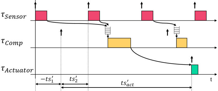
Figure 3: Data propagation from sensor to actuator. Timestamps are shown relative to the first instance of $\tau_{Comp}$.

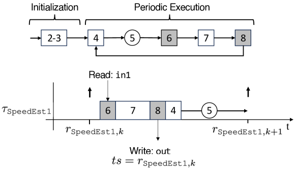
Figure 4: Control flow and execution trace of task speedEst1. Numbers refer to the line number in Listing 1, squares denote execution, and circles denote timing points.

Fig. 4 shows a diagram of the program flow (top) and execution trace (bottom) for the speed estimation. The execution trace shows an arbitrary task instance of the periodic part. The first visible timing point denotes the release of task $r_{\texttt{speedEst1},k}$. Once the task is scheduled, execution follows the sequence depicted in the program flow diagram, starting from line LABEL:lst:model:speed-read. Lines LABEL:lst:model:speed-read and LABEL:lst:model:speed-write are depicted in grey as they represent reading from and writing to a port, respectively. As there is only one call to delay in the task code and the delay is fixed to $250\text{\,}\mathrm{ms}$ (set when instantiating the task on line LABEL:lst:model:tasks1 of Fig. 2(a)), consecutive task instances are released periodically.

III-C Models and Probabilistic Constructs

We define three probabilistic constructs in ProbTime: sample, observe, and infer. We use the sample and observe when defining probabilistic models, while we use the infer construct to produce a distribution from a probabilistic model in task templates. Consider the following probabilistic model:

⬇

10def timestampToSeconds(ts : Int) : Float {

11 return intToFloat(ts) / intToFloat(1s)

12}

13model speedModel(obs : [TSV(Float)]) : Float {///\label{lst:model:model1}

14 sample b $\sim$ Uniform(0.0, maxSpeed)///\label{lst:model:intercept}

15 sample m $\sim$ Gaussian(0.0, 0.1)

16 sample sigma $\sim$ Gamma(1.0, 1.0)///\label{lst:model:sigma}

17 for o in obs {///\label{lst:model:for1}

18 var x = timestampToSeconds(timestamp(o))///\label{lst:model:tstofloat}

19 var y = m * ts + b

20 observe value(o) $\sim$ Gaussian(y, sigma)///\label{lst:model:observe}

21 }///\label{lst:model:for2}

22 return b///\label{lst:model:model-ret}

23}///\label{lst:model:model2}

This model makes use of Bayesian linear regression to estimate the speed of the train at the current logical time. On lines LABEL:lst:model:model1-LABEL:lst:model:model2, we declare the probabilistic model speedModel. The parameter obs is a sequence of speed observations encoded as a sequence of floating-point messages (we use TSV as a short-hand for timestamped values).

In this model, we use a sample statement to sample a random slope and intercept of the line. There are three latent variables (defined on lines LABEL:lst:model:intercept-LABEL:lst:model:sigma): b (the offset of the line), m (the slope of the line), and sigma (the variance, approximating the uncertainty of the estimate). The estimated line can be seen as a function over (relative) time, where $0$ is the logical time of the task instance. Consider the sample statement on line LABEL:lst:model:intercept. Here, b is the new random variable, and Uniform(0.0, maxSpeed) specifies the prior distribution we sample from.

In the for-loop on lines LABEL:lst:model:for1-LABEL:lst:model:for2, we update our belief based on the speed observations. First, we translate the relative timestamp of the observed value o to a floating-point number, representing our x-value on the line (line LABEL:lst:model:tstofloat). We use the observe statement on line LABEL:lst:model:observe to update our belief. The observed value is the data of o (retrieved using value(o)), and we expect observations to be distributed according to a Gaussian distribution (centered around the y-value). The goal of this model is to estimate the speed of the train at the logical time of the task. As we use relative timestamping, this is $0$, i.e., the intercept of the line, which we return on line LABEL:lst:model:model-ret. Our use of relative timestamps in ProbTime enables us to define this rather complicated model in just a few lines of code.

Finally, recall Listing 1 at line LABEL:lst:model:speed-infer, where we use the infer statement to infer the posterior using the probabilistic model (in this case speedModel).

III-D Compiler Implementation

Fig. 5 depicts the different steps involved in the compilation of ProbTime. We use blue rounded squares to denote compiler transformations, and gray squares to represent artifacts produced when running the compiler. The compiler is implemented within the Miking framework [27] because of its good support for defining DSLs and the possibility of extending the Miking CorePPL [12] framework with real-time constructs.

We combine the ProbTime program AST with a runtime AST where we, for example, define the behavior of infer and delay. We apply an extractor on the combined AST (top center of Fig. 5) to produce an AST for each task declared in the system declaration of the program. For each task, we extract the template it is instantiated from, along with any function dependencies. This results in vastly smaller ASTs than if we use the combined AST as templates rarely use all the functions of the runtime AST. We pass the resulting task ASTs to the backend compiler individually (bottom of Fig. 5). It translates each task AST to a CorePPL program, which we compile into an executable using the CorePPL compiler. Our implementation consists of roughly 3600 lines of code.

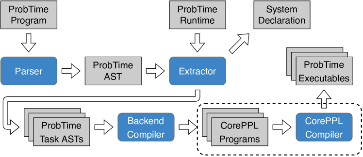
Figure 5: An overview of the ProbTime compiler. Gray square boxes represent artifacts, and rounded blue squares represent compiler transformations. In the dashed area, an existing compiler produces executable code.

IV System Model and Fairness

In this section, we present a system model, a cost model, and new perspectives on fairness that emerge when combining real-time and probabilistic inference.

IV-A System Model

A ProbTime system consists of a set of $n$ tasks $\mathcal{T}=\{\tau_{1},\ldots,\tau_{n}\}$, a set of sensors $\mathcal{S}=(s_{1},\ldots,s_{n})$ and a set of actuators $\mathcal{A}=(a_{1},\ldots,a_{n})$ as defined in the system declaration of the ProbTime program. We assume all tasks consist of an initialization followed by an infinite loop, containing one use of delay with a statically known argument. Further, to simplify our approach, we assume there is at most one use of infer in the infinite loop. This infer is the inference for which we adjust the number of particles; any uses of infer in the initialization are run using a fixed low number of particles.

While ProbTime does not syntactically restrict uses of delay, we assume all tasks are periodic and ordered by increasing period. We denote a task $\tau_{i}$ by the tuple $(C_{i},T_{i},\pi_{i},p_{i},v_{i})$, where $C_{i}$ is the worst-case execution time (WCET), $T_{i}$ is the period, $\pi_{i}$ is its static priority, $p_{i}$ is the particle count, and $v_{i}$ is its assigned importance value (recall Section III-A). Tasks are subject to an implicit deadline $D_{i}=T_{i}$. The tasks execute on an exclusive subset of the cores available on a platform. Specifically, if the platform has $m$ cores, then we schedule our tasks on a subset $\mathcal{U}=\{c_{1},\ldots,c_{k}\}$ of cores, where $k<m$ (we reserve at least one core for the platform). Each task $\tau_{i}$ is statically assigned a core $c_{j}$. We use a partitioned fixed-priority scheduling on cores $\mathcal{U}$. Priorities are assigned on the rate monotonic principle [28]. That is, $\tau_{1}$ has the highest priority $\pi_{1}$.

Each task $\tau_{i}$ has a set of predecessors $P_{i}$ such that $\tau_{j}\in P_{i}$ if $\tau_{i}$ receives data sent from an output port of $\tau_{j}$ through one of its input ports. We say that $\tau_{i}$ depends on $\tau_{j}$ if $\tau_{j}\in P_{i}$. Messages written to an output port are buffered until the finish time of a task instance, while messages are received from an input port prior to the start time of a task instance. As a consequence, communication has no impact on scheduling.

IV-B Cost model

We know that increasing the number of particles used in the inference of a task $\tau_{i}$ improves the inference accuracy leading to a better result. However, increasing the number of particles of a task $\tau_{i}$ also negatively impacts its worst-case execution time $C_{i}$. To better understand this dependency, we define the relation between the number of particles $p_{i}$ used in a task $\tau_{i}$ and the worst-case execution time $C_{i}$ as

$$C_{i}=\alpha_{i,0}+(\sum_{\tau_{j}\in P_{i}}\alpha_{i,j}\cdot p_{j})+p_{i}\cdot(\beta_{i,0}+\sum_{\tau_{j}\in P_{i}}\beta_{i,j}\cdot f(p_{j})),$$ (2)

We use the first part to represent constant-time overheads, such as reading and writing data. The term $\alpha_{i,0}$ denotes the base overhead, while the $\alpha_{i,j}$ terms represent the overhead of operating on the distributions received from predecessor tasks $\tau_{j}$ (using $p_{j}$ particles). The second part represents the execution time of the inference where we perform $p_{i}$ runs (one run per particle). We use the term $\beta_{i,0}$ to represent constant costs in the model, and the $\beta_{i,j}$ terms represent overheads of sampling from distributions of predecessors $\tau_{j}$. In particular, the function $f(p)$ encodes the cost of sampling from a distribution of $p$ particles (which is not constant-time).

IV-C Fairness

We know that more particles improve the accuracy of one inference, but we do not know how the result of one task $\tau_{i}$ impacts the behavior of the whole system. Increasing the execution time or particle counts of a task may impact the performance of other tasks. Our approach allows the user to specify how important each task is. Specifically, we use importance values $v_{i}$ associated with each task $\tau_{i}$ as a measure to guide fairness. Based on Equation (2), we define fairness in two ways: (i) execution-time fairness, where we allocate execution time budgets $b_{i}$ (which the WCETs $C_{i}$ of each task $\tau_{i}$ must not exceed) to tasks based on their importance values, and (ii) particle fairness, where fairness between tasks is given in terms of the number of particles used in the inference.

We present three scenarios to give an intuition of the differences between execution time and particle fairness. Assume we have two independent tasks $\tau_{A}$ and $\tau_{B}$ such that $T_{A}=T_{B}$ and $v_{A}=2\cdot v_{B}$, running on one core. We present the outcome of our three scenarios (labeled 1, 2, and 3, respectively) for $\tau_{A}$ and $\tau_{B}$ concerning their relative ratios of execution time and their particle count in Fig. 6. We use E to denote execution time fairness and P for particle fairness.

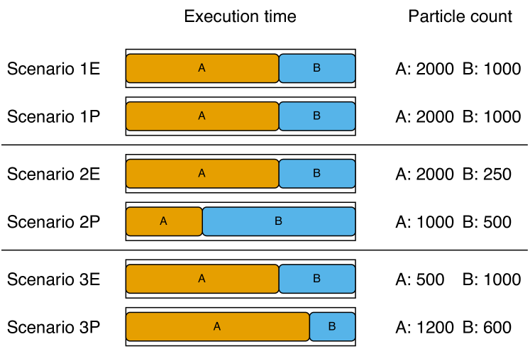
Figure 6: Illustration of execution time and particle counts for tasks $\tau_{A}$ and $\tau_{B}$ ($\tau_{A}$ is twice as important as $\tau_{B}$, using the same period) for three scenarios when considering execution time fairness (E) and particle fairness (P).

In scenario 1, the tasks are independent and require the same execution time per particle. For execution time fairness, we allocate two-thirds of the execution time to $\tau_{A}$ and one-third to $\tau_{B}$. For particle fairness, assigning $2000$ particles to $\tau_{A}$ and $1000$ particles to $\tau_{B}$ is fair. Both alternatives yield the same result as they have the same execution time per particle.

In scenario 2, we assume task $\tau_{B}$ requires four times as much execution time as $\tau_{A}$ per particle. If we use execution time fairness, the execution time of the tasks remains the same, but $\tau_{B}$ only has time to produce $250$ particles. Using particle fairness, the slowdown of $\tau_{B}$ results in both tasks producing fewer particles to maintain a fair allocation of particle counts, skewing the execution time in favor of $\tau_{B}$.

For scenario 3, we assume $\tau_{B}\in P_{A}$, i.e., that the WCET of $\tau_{A}$ depends on the particle count of $\tau_{B}$. To show this, we sketch the WCET of $\tau_{A}$ according to Equation (2) as

$$C_{A}=\ldots+p_{A}\cdot(\ldots+\beta_{A,B}\cdot f(p_{B})),$$ (3)

Using execution time fairness, we find that $\tau_{A}$ only has time to produce $500$ particles. Task $\tau_{B}$ produces the same amount of particles as in scenario 1 because it is independent of $\tau_{A}$. By contrast, when using particle fairness, $\tau_{A}$ produces more particles, and $\tau_{B}$ produces fewer.

Which kind of fairness is then preferred in a real-time probabilistic inference setting—particle fairness or execution-time fairness? Although execution-time fairness may seem natural from a real-time perspective, we will see (somewhat surprisingly) in our case study (Section VI-D) that particle fairness gives better overall accuracy.

IV-D Computation Maximization

So far, we only considered the case where tasks run on one core. What happens if we want fairness for tasks running on multiple cores? We consider two extremes: prioritizing fairness or prioritizing utilization. If we prioritize fairness, we allocate a fixed amount of resources (execution time or particles) to a task instance relative to its importance value, regardless of which core the task is mapped to. We refer to this as fair utilization. If we prioritize utilization, we maximize the utilization on each core individually without considering the importance of tasks running on other cores. We refer to this as maximum utilization. In both cases, the resulting system is schedulable.

Assume we allocate the tasks on the left-hand side of Fig. 7 on a dual-core system, such that $\tau_{A}$ and $\tau_{B}$ run on core #1 and tasks $\tau_{C}$ and $\tau_{D}$ run on core #2 (recall that $T_{i}$ is the period and $v_{i}$ is the importance of task $\tau_{i}$). On the right-hand side, we present the result of applying the two alternatives using execution time fairness (the idea also applies to particle fairness). Each box corresponds to a task instance ($\tau_{D}$ has four times the frequency of $\tau_{A}$, hence it has four boxes), and we consider the importance values to apply per task instance. We see that $\tau_{A}$ and $\tau_{B}$ are allocated the same execution time as $\tau_{A}$ is twice as important as $\tau_{B}$, but $\tau_{B}$ runs twice as frequently.

The main takeaway from Fig. 7 is that, when prioritizing fair utilization, the second core is not always fully utilized. Recall that the tasks of the system may depend on each other. By increasing the execution times of $\tau_{C}$ and $\tau_{D}$ to maximize utilization, we may negatively impact the performance of $\tau_{A}$ and $\tau_{B}$. This is unfair considering that $\tau_{A}$ and $\tau_{B}$ are given higher importance. On the other hand, if there is no such dependency, we are wasting computational resources. We propose the concept of fair utilization maximization, where we start from fair utilization and gradually increase the resources (execution time or particles) allocated to tasks on cores that are not fully utilized as long as the system remains schedulable. If $\tau_{A}$ and $\tau_{B}$ do not depend on $\tau_{C}$ and $\tau_{D}$, we get the same result as when prioritizing maximum utilization.

Task	$T_{i}$	$v_{i}$
$\tau_{A}$	$1\text{\,}\mathrm{s}$	8
$\tau_{B}$	$0.5\text{\,}\mathrm{s}$	4
$\tau_{C}$	$1\text{\,}\mathrm{s}$	4
$\tau_{D}$	$0.25\text{\,}\mathrm{s}$	2

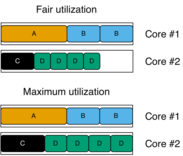
Figure 7: The resulting utilization of the tasks (left) allocated on two cores when prioritizing fairness (top right) or maximizing the utilization (bottom right) in terms of execution time.

V Automatic Configuration

In this section, we present two approaches to automatic configuration that we apply to a compiled ProbTime system to maximize inference accuracy while preserving schedulability.

V-A Configuration Overview

We define two key phases needed to configure a ProbTime system: (i) the collection phase, where we record sensor inputs, and (ii) the configuration phase, where we determine the particle counts of all tasks. During phase (i), we collect input data from the sensors of the real system, which we replay repeatedly during (ii) in a hardware-in-the-loop simulation. The configuration phase is specific to the hardware it runs on, so we need to run phase (ii) on the same hardware as we intend to run the configured system on. Our discussion is focused on the configuration phase (ii).

We present two alternative approaches to automatic configuration based on execution time fairness (Section V-B) and particle fairness (Section V-C). In both cases, we seek a particle count $p_{i}$ to use in the inference of each task $\tau_{i}$ based on its importance value $v_{i}$, using fair utilization. For simplicity, we assume the user provides a task-to-core mapping $\mathcal{M}$ specifying on which core each task runs (such that $\mathcal{M}_{\tau}\in\mathcal{U}$). Also, we assume we have a function RunTasks that runs the ProbTime system with recorded sensor data to measure the WCET of each task. Finally, we use a configurable safety margin factor $\delta$ (set to $0.9$ in our implementation) to protect against outliers.

Algorithm 1 Function to compute the number of particles to use for execution-time fairness.

1:procedure ComputeBudgets($\mathcal{M},\mathcal{T}$)

2:    for $c_{i}\in\mathcal{U}$ do

3:        $\mathbf{d}\leftarrow\{v_{j}\ |\ \tau_{j}\in\mathcal{T}\land\mathcal{M}_{\tau_{j}}=c_{i}\}$

4:        $\lambda_{i}\leftarrow\textsc{SensitivityAnalysis}(\mathbf{d})$     

5:    $\lambda\leftarrow\min_{i}\lambda_{i}$

6:    $\mathbf{return}\ \{v_{i}\cdot\lambda\ |\ \tau_{i}\in\mathcal{T}\}$

7:procedure Configure_EF($\mathcal{M},\mathcal{T}$)

8:    $L\leftarrow\{(\tau_{i},1)\ |\ \tau_{i}\in\mathcal{T}\}$

9:    $U\leftarrow\{(\tau_{i},\infty)\ |\ \tau_{i}\in\mathcal{T}\}$

10:    $A\leftarrow\{\tau_{i}\ |\ \tau_{i}\in\mathcal{T}\land P_{i}=\emptyset\}$

11:    $b\leftarrow\textsc{ComputeBudgets}(\mathcal{M},\mathcal{T})$

12:    $F\leftarrow\emptyset$

13:    while $A\neq\emptyset$ do

14:        $W\leftarrow\textsc{RunTasks}(\mathcal{M},\mathcal{T})$

15:        for $\tau_{i}\in A$ do

16:           if $L_{i}+1<U_{i}$ then

17:               $L_{i},U_{i}\leftarrow\begin{cases}L_{i},p_{i}&\text{if }W_{i}>b_{i}\cdot\delta\\ p_{i},U_{i}&\text{otherwise}\end{cases}$

18:               $p_{i}\leftarrow\begin{cases}2\cdot L_{i}&\text{if }U_{i}=\infty\\ \frac{L_{i}+U_{i}}{2}&\text{otherwise}\end{cases}$

19:           else

20:               $p_{i}\leftarrow L_{i}$

21:               $F\leftarrow F\cup\{\tau_{i}\}$                    

22:        $A\leftarrow\{\tau_{i}\ |\ \tau_{i}\in\mathcal{T}\land P_{i}\subseteq F\}\setminus F$     

23:    $\mathbf{return}\ \mathcal{T}$

V-B Execution Time Fairness

We perform two steps to achieve execution time fairness. First, we compute fair execution time budgets $b_{i}$ for all tasks $\tau_{i}$ based on their importance $v_{i}$, such that all tasks remain schedulable. Second, we maximize the particle counts $p_{i}$ while ensuring the WCET $C_{i}$ of each task is below its budget $b_{i}$.

We define the ComputeBudgets function in Algorithm 1 (lines 1-6) to compute the execution time budgets of tasks with fair utilization. As our approach assumes partitioned scheduling, we can examine tasks assigned to different cores separately. For each core $c_{i}$, we use the sensitivity analysis in the C-space by Bini et al. [29] to compute a maximum change $\lambda_{i}$ to the execution times of tasks for which they remain schedulable, given a direction vector $\mathbf{d}$ (initially, we assume all execution times are zero). We define $\mathbf{d}$ based on the importance values of the tasks (line 3) and apply this to the SensitivityAnalysis function to compute the $\lambda_{i}$ (line 4). We pick the minimum lambda among all cores on line 5 and use this to get fair execution time budgets for all tasks on line 6.

We use the execution time budgets $b$ as an upper bound for the WCET of the task $\tau_{i}$ while trying to maximize its particle count $p_{i}$. We need to carefully adjust the particle counts of tasks, as tasks may depend on each other. Assume we find a maximum particle count $p_{i}$ for a task $\tau_{i}$. If we increase the number of particles of one of the predecessors $\tau_{j}$ of $\tau_{i}$, this may cause the execution time of $\tau_{i}$ to increase according to Equation (2). Observe that if we keep the particle count of all predecessors of a task fixed, we can consider the $\alpha_{i,j}\cdot p_{j}$ and $\beta_{i,j}\cdot f(p_{j})$ terms as constant. As long as we keep the particle counts of all predecessors of a task $\tau_{i}$ fixed, the WCET $C_{i}$ is directly proportional to its particle count $p_{i}$. This means we can binary search to find the maximum $p_{i}$.

We use these observations in the Configure_EF function of Algorithm 1. We keep track of a set of active tasks $A$ with no predecessors (initialized on line 10). While we have active tasks, we use the RunTasks function to measure the WCETs of all tasks $W$ (line 14). We keep track of lower and upper bounds, $L_{i}$ and $U_{i}$, of the particle count for each task $\tau_{i}$. For each active task $\tau_{i}$, we run an iteration of binary search by comparing its WCET estimate to its budget and update the bounds accordingly (lines 16-21). When the binary search concludes, we set the particle count to the lower bound and add the task to a set of finished tasks $F$ (lines 20-21). After each iteration, we update the set of active tasks to be the unfinished tasks with no unfinished predecessors (line 22). When the active set $A$ is empty, we have found a particle count to use for all tasks, and we return the updated task set $\mathcal{T}$ (line 23). Our approach works under the assumption that the system definition graph is acyclic.

V-C Particle Fairness

Algorithm 2 Computing the number of particles to use for particle fairness.

1:procedure Schedulable($\mathcal{M},\mathcal{T},k$)

2:    for $\tau_{i}\in\mathcal{T}$ do

3:        $p_{i}\leftarrow v_{i}\cdot k$     

4:    $W\leftarrow\textsc{RunTasks}(\mathcal{M},\mathcal{T})$

5:    for $\tau_{i},w_{i}\in W$ do

6:        $C_{i}\leftarrow\frac{w_{i}}{\delta}$     

7:    $\textbf{return}\ \textsc{RTA}(\mathcal{M},\mathcal{T})$

8:procedure Configure_PF($\mathcal{M},\mathcal{T}$)

9:    $l\leftarrow 1$

10:    $u\leftarrow\infty$

11:    while $l+1<u$ do

12:        $k\leftarrow\begin{cases}2\cdot l&\text{if }u=\infty\\ \frac{l+u}{2}&\text{otherwise}\end{cases}$

13:        $l,u\leftarrow\begin{cases}k,u&\text{if }\textsc{Schedulable}(\mathcal{M},\mathcal{T},k)\\ l,k&\text{otherwise}\end{cases}$     

14:    for $\tau_{i}\in\mathcal{T}$ do

15:        $p_{i}\leftarrow l\cdot v_{i}$     

16:    $\textbf{return}\ \mathcal{T}$

For particle fairness, we seek a multiple $k$ such that $p_{i}=k\cdot v_{i}$ for all tasks $\tau_{i}$. Note that when we increase the value of $k$, the execution time of all tasks increases according to Equation (2), meaning we can binary search to find the maximum $k$. For a fixed value $k$, we need to determine whether the tasks are schedulable. We do this in the Schedulable function on lines 1-7 of Algorithm 2. Before running the tasks on line 4, we set the number of particles for each taskWe set the WCETs the tasks based on the observations from running them (lines 5-6). Finally, on line 7, we perform a response time analysis to ensure the tasks are schedulable.

We use the Schedulable function in the particle fairness function Configure_PF (lines 8-16). We define the lower and upper bounds $l$ and $u$ on lines 9-10, and we binary search in this interval on lines 11-13. After the loop, the maximum multiple for which the system is schedulable is stored in $l$. We set the particle count $p_{i}$ of each task $\tau_{i}$ on lines 14-15 before returning the updated task set on line 16.

VI Automotive Case Study

To demonstrate the applicability of ProbTime to program time-critical embedded systems, we develop a case study for a localization pipeline in an automotive testbed. This section first introduces the testbed, followed by an evaluation of ProbTime.

VI-A Automotive Testbed

The automotive industry is undergoing a paradigm shift to face the challenges that emerge through the advent of autonomous driving [30]. These challenges require higher computational capacities and larger communication bandwidth compared to traditional automotive systems. This transition leads to a software-defined vehicle where almost all functions of the car will be enabled by software [31]. In order to demonstrate the applicability of our proposed methods in this context, we have developed an automotive testbed.

VI-A1 Hardware

The testbed is designed around a 1:10 scale RC car. The E/E architecture consists of a number of distributed compute nodes of different characteristics that are connected via bus- and network-based interconnects (see Fig. 8).

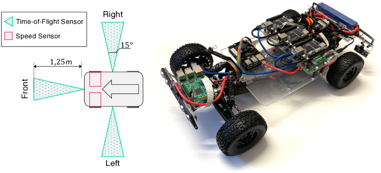
Figure 8: Overview of the sensors on the car (left) and a picture of the RC-Car testbed (right).

Two microcontroller-based compute nodes act as the interface to most actuators and sensors of the car. High-performance compute nodes provide the required performance to host computation required for Advanced Driving Assistance (ADAS) or Autonomous Driving (AD) workloads. We use a Raspberry Pi 4B (4 Cortex-A72 cores at 1.5GHz). These compute nodes are connected by a local Ethernet network.

We use three Time-of-Flight (TOF) sensors installed at the front and on the left and right sides of the car, as indicated in Fig. 8. These sensors have high accuracy, but they can only measure distances up to $1.25~{}\text{m}$. The front wheel sensors report the current speed of the car.

VI-A2 Software

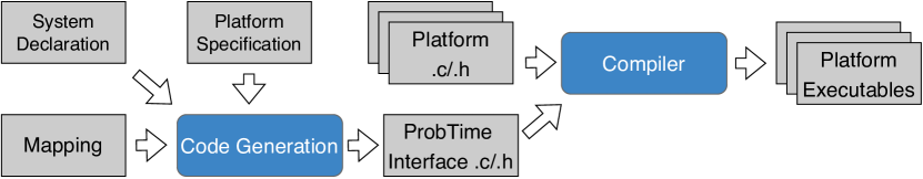
Figure 9: Code generation and compilation of the platform code, including a ProbTime interface.

The operating system on the Raspberry Pi 4B compute node is Linux-based with kernel 5.15.55-rt48-v8+ SMP PREEMPT_RT. The platform software is responsible for reading sensor data and controlling actuators. This is realized by dedicated periodic tasks that are distributed on different compute nodes. Each task is assigned a static priority and is mapped to a CPU core. Platform software realizes communication between ProbTime tasks, realized by communication buffers located in shared memory. Additionally, sensor data is written to the ProbTime communication buffer and from the communication buffer to actuators.

We use code generation to generate necessary files that realize the interface to a specific ProbTime program (see Fig. 9). Input to the code generation is the system declaration, describing the ProbTime program. The remaining platform software is not affected by code generation. In the final step, the compiler produces an executable for each compute node.

VI-B Evaluation Questions

To evaluate ProbTime and our automatic configuration, we pose the following evaluation questions:

1. To what extent can ProbTime’s timing and probabilistic constructs be used to implement a realistic application?

2. What is the trade-off between the number of particles, execution time, and inference accuracy, and how does it relate to the cost model of Equation (2)?

3. When configuring without prior knowledge of runtime characteristics, how does the result of execution time fairness compare to particle fairness with respect to inference accuracy and timing properties?

4. To what extent and accuracy can the case study—when executed on the physical car—determine the position and avoid collision?

VI-C Positioning and Braking in ProbTime (Q1)

We implement a positioning and braking system in ProbTime as a case study. The system estimates the position of the RC car while it is moving using sensor inputs. Further, the system reacts by braking to prevent collisions with obstacles.

We present an overview of our positioning and braking system in Fig. 10. We show our sensor inputs on the left-hand side. The steering angle is an input signal from the controller, while the other five sensors are directly related to sensors on the car (as shown in Fig. 8). We use the brake actuator (right-hand side) to activate the emergency brakes.

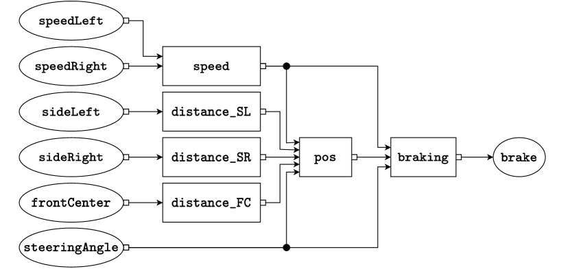
Figure 10: A graphical representation of the system declaration we use for our positioning and braking system.

The squares of Fig. 10 represent the tasks. Note that we instantiate the distance estimation tasks (distance_SL, distance_SR, and distance_FC) from the same template. These three tasks do not perform any inference. All tasks have a period of $500\text{\,}\mathrm{ms}$ except pos, which has a period of $1\text{\,}\mathrm{s}$.

We use the speed task to estimate the car’s average speed since the last estimation, based on speed observations from the wheels. We found that the speed sensors on the car are inaccurate at low speeds and that the car reaches its top speed almost instantaneously at max throttle. We assume the car is in one of three states: stationary, max speed, or transitioning (where we are uncertain of the average speed).

Our positioning task estimates the x- and y-coordinates of the center of the car. It also estimates the direction the car is facing, relative to an encoded map of the environment (provided by the user). The model starts from a prior belief of the position (initially, a known starting position) and estimates a trajectory along which the car moved until the logical time of the task, based on steering angle observations and speed estimations. We update our belief by comparing each input distance estimation with what the sensor would have observed at that timestamp, given that the car followed the estimated trajectory. We implement this using Bayesian linear regression (as in our example of Section III-C). The braking task uses a model to estimate the distance until a collision takes place, given steering angle observations, an encoded map, and the speed and position estimations. If the median distance is below a fixed threshold, we activate the emergency brakes.

In summary, in response to Q1, the current case study demonstrates that a highly non-trivial application can be efficiently implemented using our proposed RTPPL DSL. In total, the case study consists of 600 lines of ProbTime code.

VI-D Experiments and Results

To answer evaluation questions Q2, Q3, and Q4, we perform three experiments using our positioning and braking models. We run the first two experiments in a simulation by replaying observed sensor inputs, on an Intel(R) Xeon(R) Gold 6148 CPU with 64 GB RAM using Ubuntu 22.04. The third experiment is performed on the RC car. We only consider the speed, pos, and braking tasks when discussing results or settings for individual tasks, as the distance estimation tasks perform no inference.

VI-D1 Positioning Inference Accuracy (Q2)

We investigate how the inference accuracy and execution times are impacted when increasing the number of particles. To allow us to run more particles per inference, we perform a slow mode simulation where the data replaying, and the ProbTime tasks consider time to pass slower relative to the wall time. We use position estimates as a measure of inference accuracy because we can compute the error of the final position estimate relative to a known final position, using pre-recorded input data. In our experiments, we vary the particle count of the pos task while fixing the particle count of speed and braking to $1000$.

In Fig. 11, we present the average position error (left) and WCETs (right) for the three tasks over $50$ runs with varying particle counts in the positioning task. Note that the positioning model often fails to track the car at all when using $10^{2}$ particles. As we increase the number of particles from $10^{2}$ to $10^{3}$, the estimation error decreases drastically. When we increase the particle count further, the average error decreases, and the variance lowers slightly. We believe the increased error when going from $10^{4}$ to $10^{5}$ particles is due to inaccuracies in our model (for example, it approximates the room as 10x10 cm squares). Observe that the WCETs are consistent with the cost model of Equation (2). The WCET of the speed task is more or less constant because it is independent of the pos task, while the braking task depends on pos and is therefore slowed down as we increase the particle count of the pos task. Finally, the execution time of the pos task increases linearly with increasing particle counts.

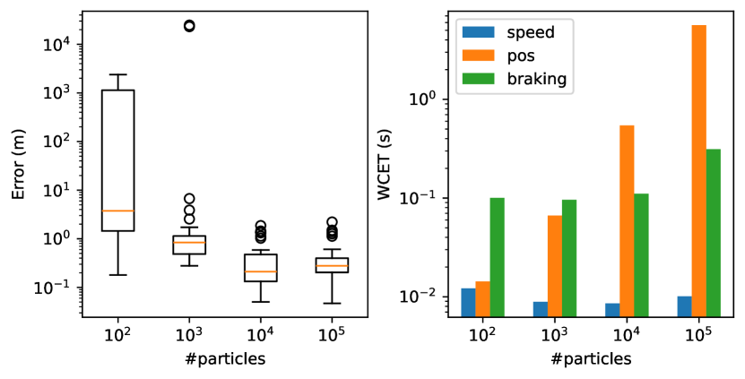
Figure 11: Results showing the average expected distance (logarithmic scale) over ten runs when varying the number of particles in the positioning model.

VI-D2 Automatic Configuration (Q3)

For this experiment, we assume no knowledge of the runtime characteristics of our ProbTime system. Therefore, we do not know what importance values to assign to our tasks. We argue that a reasonable starting point is to give all tasks the same importance. We allocate the speed, pos, and braking tasks to one core and assign them an importance value of $1$. We perform the configuration using execution time fairness and particle fairness and compare the configured systems in terms of inference accuracy (of the positioning model), the number of particles, the WCET, and the average utilization of the three tasks (measured using ps -p <pid> -o %cpu).

We present the results using execution time fairness (EF) and particle fairness (PF) for the speed, pos, and braking tasks in Table I. At the top, we present the inference accuracy (as average position error $\pm$ standard deviation). In the lower part, we show the particle count (P) of the configured system and the average WCET and utilization (U) for each task over ten runs of the configured system. Recall that the period of pos is $1\text{\,}\mathrm{s}$, whereas the speed and braking tasks have a period of $500\text{\,}\mathrm{ms}$, meaning they run twice as often as pos.

We see that the task WCETs are similar when using execution time fairness. However, the particle counts are unbalanced, with the speed task using two orders of magnitude more particles than pos and braking. As the speed task uses a simple model, it has time to infer many particles. Because the pos and braking tasks depend on the output of speed, they are slowed down significantly due to the sampling overheads. However, when we use particle fairness, all tasks are assigned the same particle count. As speed produces particles faster than the other tasks, its WCET and utilization are very low. More importantly, we see that the resulting inference accuracy is significantly better using particle fairness.

These findings suggest that particle fairness is preferable to execution time fairness. Using trial and error, we may achieve a balance of particles using either approach, but task dependencies make it difficult to predict the outcome when using execution time fairness.

TABLE I: The inference accuracy of the positioning model and the average particle count (P), WCET, and utilization (U) per task of our ProbTime system when configured using execution time fairness (EF) and particle fairness (PF).

	EF			PF
Accuracy	$1.32\pm 0.94$			$0.53\pm 0.50$
Task	P	WCET	U	P	WCET	U
speed	97283	0.195	0.311	3062	0.013	0.016
pos	157	0.186	0.153	3062	0.156	0.107
braking	509	0.179	0.292	3062	0.382	0.310

VI-D3 Positioning and Braking (Q4)

Figure 12: The encoded map ($18.6\text{\,}\mathrm{m}$ x $9.5\text{\,}\mathrm{m}$) of the corridor in which we drive the car. The overlay shows particles spreading when less information is available (top-right) and gathering when close to obstacles (bottom left).

For this experiment, we run the ProbTime tasks on the car. To evaluate the positioning model, we drive full laps around the office corridor of our building (see Fig. 12). Observe how the cloud of particles in Fig. 12 spreads out when less information is available (top-right) and gathers when the sensors are close to obstacles (bottom-left).

As we cannot measure the car’s position while moving, we start it from a known initial position and compare our manual measurement of the final position with the expected position according to the positioning model. We drive the car in a clockwise direction for a full lap ten times using two scenarios. In the first scenario, we start at the bottom-left corner and drive past the starting point (near the objects). In the second scenario, we start in the top-right corner and stop in the long corridor at the top. Using trial and error, we found using importance $40$ for pos and $10$ for speed and braking to yield good results. The configured system uses $1080$ particles in pos and $270$ in the other two.

We evaluate the automated braking by driving the car around in the corridor. We found that the emergency brakes are conservative – while they prevent collisions, they often activate in situations where it is unnecessary. This is due to uncertainty in the position estimations. Due to the conservative nature of the braking task, we disable the brake actuator when evaluating the positioning model.

We present our positioning results in Table II. In one run of scenario 2, the task lost track of the car during the upper-right corner, so we use the last valid estimation instead. We present scenario 2* where that run is excluded. Observe that the x-axis error is small in scenario 2 because both side sensors are in range, while the y-error is larger because the front sensor makes no observations in range. Despite the short range of our sensors, the lack of distinguishing details in the environment, and the limited computational capacity of the car testbed, our model successfully manages to track the car for a full lap.

TABLE II: Results showing the average error in the x- and y- direction as well as the Euclidean distance for our two scenarios, with standard deviations.

Scenario	x-axis error	y-axis error	Euclidean distance
1	$0.44\pm 0.28$	$0.22\pm 0.30$	$0.51\pm 0.38$
2	$1.13\pm 2.06$	$0.18\pm 0.13$	$1.18\pm 2.05$
2*	$0.51\pm 0.61$	$0.15\pm 0.07$	$0.55\pm 0.59$

VII Related Work

Although surprisingly little has been done in the intersection of probabilistic programming and languages for real-time systems, there is a large body of work in each category. This section gives a brief summary of the closest related work.

Probabilistic programming languages. Languages for performing Bayesian inference date back to the early 1990s, where BUGS [32] is one of the earliest languages for Bayesian networks. The term probabilistic programming was coined much later but is now used in general for all languages performing Bayesian inference. Starting with the Church language [33], a new, more general form of probabilistic programming languages emerged, called universal PPLs. In such languages, the probabilistic model is encoded in a Turing complete language, which enables stochastic branching and possibly an infinite number of random variables. There exist many experimental PPLs in this category, e.g., Gen [11], Anglican [9], Turing [10], WebPPL [7], Pyro [6], and CorePPL [12]. Other state-of-the-art PPL environments are, e.g., Stan [8] and Infer.NET. Similar to many of these environments, ProbTime also makes use of the standard core constructs (sample, observe, and infer), where the key difference is that time and timeliness are also taken into consideration in ProbTime.

Real-time programming languages. There exists a quite large body of literature on programming languages that incorporate time and timing as part of the language semantics. Ada [19] has explicit support for timed language constructs, and the real-time extension to Java [34] supports time and event handling. Recently, Timed C was proposed in the research literature as a way to incorporate timing constructs directly in the language. The Timed C work has later been extended to also support sensitive analysis [35]. Our work has been inspired by Timed C, and the semantics for delay constructs is derived from Timed C, although the implementation is different. However, in contrast to Timed C, ProbTime also introduces tagging with timestamps. There are several other languages and environments that have timestamped and tagged values as central semantic concepts. For instance, PTIDES [36] is an extension to the discrete-event (DE) model. Lingua Franca [18] is another recent effort that introduces deterministic actors called reactors, whose only means of communication is through an ordered set of reactions.

Synchronous programming. There are also other approaches to programming real-time systems, where time is abstracted as ticks. Specifically, the synchronous programming paradigm [37] implements such an approach, where ProbZelus [20] is a recent programming language extending synchronous reactive programming with probabilistic constructs. The ProbZelus work is based on the delayed sampling concept [38] to automatically make inference efficient when conjugate priors can be exposed in the model. A key difference between ProbZelus and our work is in how time is handled. In our work, real-time is first class, and the timing data (timestamped data) can be used as part of the model, relaxing the need to have periodic data that arrives in a synchronous fashion.

Reward-based scheduling. Our approach to configuration is related to reward-based scheduling [39], where tasks consist of a mandatory and an optional part. A non-decreasing reward function maps the time spent running the optional part to a real value. The goal of this approach is to find a schedule for which we maximize the reward while all tasks remain schedulable. In ProbTime, inference is the optional part of tasks as we can vary how many particles we use, where the importance values assigned to tasks implicitly encode a reward function.

VIII Conclusion

In this paper, we introduce a new kind of language called real-time probabilistic programming language (RTPPL). To demonstrate this new kind of language, we develop the first domain-specific RTPPL called ProbTime. We also introduce the concepts of fairness in RTPPLs and demonstrate the strength of particle fairness.

References

- [1] A. D. Gordon, T. A. Henzinger, A. V. Nori, and S. K. Rajamani, “Probabilistic programming,” in Proceedings of the on Future of Software Engineering. ACM, 2014, pp. 167–181.
- [2] J.-W. van de Meent, B. Paige, H. Yang, and F. Wood, “An introduction to probabilistic programming,” arXiv preprint arXiv:1809.10756, 2018.
- [3] A. Doucet, N. De Freitas, and N. Gordon, “An introductiona to sequential Monte Carlo methods,” Sequential Monte Carlo methods in practice, pp. 3–14, 2001.
- [4] Lundén, Daniel and Borgström, Johannes and Broman, David, “Correctness of Sequential Monte Carlo Inference for Probabilistic Programming Languages,” in Proceedings of 30th European Symposium on Programming (ESOP), ser. LNCS, vol. 12648. Springer, 2021, pp. 404–431.
- [5] S. Brooks, “Markov chain Monte Carlo method and its application,” Journal of the royal statistical society: series D (the Statistician), vol. 47, no. 1, pp. 69–100, 1998.
- [6] E. Bingham, J. P. Chen, M. Jankowiak, F. Obermeyer, N. Pradhan, T. Karaletsos, R. Singh, P. Szerlip, P. Horsfall, and N. D. Goodman, “Pyro: Deep Universal Probabilistic Programming,” Journal of Machine Learning Research, vol. 20, no. 28, pp. 1–6, 2019.
- [7] N. D. Goodman and A. Stuhlmüller, “The Design and Implementation of Probabilistic Programming Languages,” http://dippl.org/ [Last accessed: May 17, 2023].
- [8] B. Carpenter, A. Gelman, M. D. Hoffman, D. Lee, B. Goodrich, M. Betancourt, M. Brubaker, J. Guo, P. Li, and A. Riddell, “Stan: A probabilistic programming language,” Journal of Statistical Software, vol. 76, no. 1, 2017.
- [9] D. Tolpin, J.-W. van de Meent, H. Yang, and F. Wood, “Design and implementation of probabilistic programming language anglican,” in Proceedings of the 28th Symposium on the Implementation and Application of Functional Programming Languages, ser. IFL 2016. New York, NY, USA: ACM, 2016, pp. 6:1–6:12.
- [10] H. Ge, K. Xu, and Z. Ghahramani, “Turing: a language for flexible probabilistic inference,” in International conference on artificial intelligence and statistics (AISTATS). PMLR, 2018, pp. 1682–1690.
- [11] M. F. Cusumano-Towner, F. A. Saad, A. K. Lew, and V. K. Mansinghka, “Gen: a general-purpose probabilistic programming system with programmable inference,” in Proceedings of the 40th ACM SIGPLAN Conference on Programming Language Design and Implementation (PLDI). ACM, 2019, pp. 221–236.
- [12] Lundén, Daniel and Öhman, Joey and Kudlicka, Jan and Senderov, Viktor and Ronquist, Fredrik and Broman, David, “Compiling Universal Probabilistic Programming Languages with Efficient Parallel Sequential Monte Carlo Inference,” in Proceedings of 31th European Symposium on Programming (ESOP), 2022, pp. 29–56.
- [13] A. Lew, M. Agrawal, D. Sontag, and V. Mansinghka, “PClean: Bayesian data cleaning at scale with domain-specific probabilistic programming,” in International Conference on Artificial Intelligence and Statistics (AISTATS). PMLR, 2021, pp. 1927–1935.
- [14] F. Ronquist, J. Kudlicka, V. Senderov, J. Borgström, N. Lartillot, D. Lundén, L. Murray, T. B. Schön, and D. Broman, “Universal probabilistic programming offers a powerful approach to statistical phylogenetics,” Communications Biology, vol. 4, no. 1, pp. 1–10, 2021.
- [15] N. Gothoskar, M. Cusumano-Towner, B. Zinberg, M. Ghavamizadeh, F. Pollok, A. Garrett, J. Tenenbaum, D. Gutfreund, and V. Mansinghka, “3DP3: 3D Scene Perception via Probabilistic Programming,” Advances in Neural Information Processing Systems (NeurIPS), vol. 34, pp. 9600–9612, 2021.
- [16] N. D. Goodman, J. B. Tenenbaum, and T. P. Contributors, “Probabilistic Models of Cognition,” 2016, (2nd ed.) https://probmods.org/ [Last accessed: May 17, 2023].
- [17] S. Natarajan and D. Broman, “Timed C: An Extension to the C Programming Language for Real-Time Systems,” in Proceedings of IEEE Real-Time and Embedded Technology and Applications Symposium (RTAS), 2018.
- [18] M. Lohstroh, C. Menard, S. Bateni, and E. A. Lee, “Toward a Lingua Franca for Deterministic Concurrent Systems,” ACM Transactions on Embedded Computing Systems (TECS), vol. 20, no. 4, pp. 1–27, 2021.
- [19] A. Burns and A. Wellings, Concurrent and real-time programming in Ada. Cambridge University Press, 2007.
- [20] G. Baudart, L. Mandel, E. Atkinson, B. Sherman, M. Pouzet, and M. Carbin, “Reactive Probabilistic Programming,” in Proceedings of the 41st ACM SIGPLAN Conference on Programming Language Design and Implementation (PLDI), 2020, pp. 898–912.
- [21] G. Baudart, L. Mandel, and R. Tekin, “Jax based parallel inference for reactive probabilistic programming,” in Proceedings of the 23rd ACM SIGPLAN/SIGBED International Conference on Languages, Compilers, and Tools for Embedded Systems, 2022, pp. 26–36.
- [22] A. Pfeffer, “Ctppl: A continuous time probabilistic programming language.” in IJCAI, 2009, pp. 1943–1950.
- [23] D. Broman, “A Vision of Miking: Interactive Programmatic Modeling, Sound Language Composition, and Self-Learning Compilation,” in Proceedings of the 12th ACM SIGPLAN International Conference on Software Language Engineering, ser. SLE ’19. ACM, 2019, pp. 55–60.
- [24] F. Gustafsson, F. Gunnarsson, N. Bergman, U. Forssell, J. Jansson, R. Karlsson, and P.-J. Nordlund, “Particle filters for positioning, navigation, and tracking,” IEEE Transactions on signal processing, vol. 50, no. 2, pp. 425–437, 2002.
- [25] C. A. Naesseth, F. Lindsten, T. B. Schön et al., “Elements of sequential monte carlo,” Foundations and Trends® in Machine Learning, vol. 12, no. 3, pp. 307–392, 2019.
- [26] C. M. Kirsch and A. Sokolova, “The logical execution time paradigm,” in Advances in Real-Time Systems (to Georg Färber on the occasion of his appointment as Professor Emeritus at TU München after leading the Lehrstuhl für Realzeit-Computersysteme for 34 illustrious years), S. Chakraborty and J. Eberspächer, Eds. Springer, 2012, pp. 103–120.
- [27] D. Broman, “A vision of miking: Interactive programmatic modeling, sound language composition, and self-learning compilation,” in Proceedings of the 12th ACM SIGPLAN International Conference on Software Language Engineering, SLE 2019, Athens, Greece, October 20-22, 2019, O. Nierstrasz, J. Gray, and B. C. d. S. Oliveira, Eds. ACM, 2019, pp. 55–60.
- [28] C. L. Liu and J. W. Layland, “Scheduling algorithms for multiprogramming in a hard-real-time environment,” Journal of the ACM (JACM), vol. 20, no. 1, pp. 46–61, 1973.
- [29] E. Bini, M. Di Natale, and G. Buttazzo, “Sensitivity analysis for fixed-priority real-time systems,” Real-Time Systems, vol. 39, pp. 5–30, 2008.
- [30] D. Zerfowski and D. Buttle, “Paradigm shift in the market for automotive software,” ATZ worldwide, vol. 121, no. 9, pp. 28–33, 2019.
- [31] H. Windpassinger, “On the way to a software-defined vehicle,” ATZelectronics worldwide, vol. 17, no. 7, pp. 48–51, 2022.
- [32] W. R. Gilks, A. Thomas, and D. J. Spiegelhalter, “A language and program for complex Bayesian modelling,” The Statistician, vol. 43, no. 1, pp. 169–177, 1994.
- [33] N. D. Goodman, V. K. Mansinghka, D. Roy, K. Bonawitz, and J. B. Tenenbaum, “Church: A language for generative models,” in Proceedings of the Twenty-Fourth Conference on Uncertainty in Artificial Intelligence, ser. UAI’08. Arlington, Virginia, United States: AUAI Press, 2008, pp. 220–229.
- [34] G. Bollella and J. Gosling, “The real-time specification for java,” Computer, vol. 33, no. 6, pp. 47–54, 2000.
- [35] S. Natarajan, M. Nasri, D. Broman, B. B. Brandenburg, and G. Nelissen, “From code to weakly hard constraints: A pragmatic end-to-end toolchain for Timed C,” in Proccedings of the IEEE Real-Time Systems Symposium (RTSS). IEEE, 2019, pp. 167–180.
- [36] J. C. Eidson, E. A. Lee, S. Matic, S. A. Seshia, and J. Zou, “Distributed real-time software for cyber–physical systems,” Proceedings of the IEEE, vol. 100, no. 1, pp. 45–59, 2011.
- [37] A. Benveniste and G. Berry, “The Synchronous Approach to Reactive and Real-Time Systems,” Proc. of the IEEE, vol. 79, no. 9, pp. 1270–1282, 1991.
- [38] L. Murray, D. Lundén, J. Kudlicka, D. Broman, and T. Schön, “Delayed Sampling and Automatic Rao-Blackwellization of Probabilistic Programs,” in Proceedings of Machine Learning Research : International Conference on Artificial Intelligence and Statistics (AISTATS). PMLR, 2018.
- [39] H. Aydin, R. Melhem, D. Mossé, and P. Mejia-Alvarez, “Optimal reward-based scheduling for periodic real-time tasks,” IEEE Transactions on Computers, vol. 50, no. 2, pp. 111–130, 2001.