Accretion-modified Stars in Accretion Disks of Active Galactic Nuclei: the Low-luminosity Cases and an Application to Sgr A$\!{}^{*}$ 

Abstract

In this paper, we investigate the astrophysical processes of stellar-mass black holes (sMBHs) embedded in advection-dominated accretion flows (ADAFs) of supermassive black holes (SMBHs) in low-luminosity active galactic nuclei (AGNs). The sMBH is undergoing Bondi accretion at a rate lower than the SMBH. Outflows from the sMBH-ADAF dynamically interact with their surroundings and form a cavity inside the SMBH-ADAF, thereby quenching the accretion onto the sMBH. Rejuvenation of the Bondi accretion is rapidly done by turbulence. These processes give rise to quasi-periodic episodes of sMBH activities and creat flickerings from relativistic jets developed by the Blandford-Znajek mechanism if the sMBH is maximally rotating. Accumulating successive sMBH-outflows trigger viscous instability of the SMBH-ADAF, leading to a flare following a series of flickerings. Recently, the similarity of near-infrared flare’s orbits has been found by GRAVITY/VLTI astrometric observations of Sgr A$\!{}^{*}$: their loci during the last 4-years consist of a ring in agreement with the well-determined SMBH mass. We apply the present model to Sgr A$\!{}^{*}$ , which shows quasi-periodic flickerings. An sMBH of $\sim 40M_{\odot}$ is preferred orbiting around the central SMBH of Sgr A$\!{}^{*}$ from fitting radio to X-ray continuum. Such an extreme mass ratio inspiraling (EMRI) provides an excellent laboratory for LISA / Taiji / Tianqin detection of mHz gravitational waves with strains of $\sim 10^{-17}$, as well as their polarization.

1 Introduction

The model of accretion onto a single supermassive black hole (SMBH) is successful to explain the powerful radiation of active galactic nuclei (AGNs) (e.g., Rees, 1984), however, there is a growing body of evidence suggesting that some new ingredients should be incorporated into this canonical model. Star formation has been suggested by many authors for different purposes since the early attempts of Kolykhalov & Sunyaev (1980) in light of the self-gravity of outer parts of the AGN accretion disks (Paczyński, 1978). Consequently, it may be an efficient way of fueling gas to galactic centers, triggering the activity of SMBHs (Shlosman & Begelman, 1989; Thompson et al., 2005; Wang et al., 2010). Spectral energy distributions of AGNs could be revised by star formation (Goodman, 2003; Goodman & Tan, 2004; Thompson et al., 2005) as well as the origins of high metallicity (Collin & Zahn, 1999, 2008; Wang et al., 2011, 2012b; Grishin et al., 2021; Wang et al., 2023; Fan & Wu, 2023) observed in AGN broad-line regions (Hamann & Ferland, 1999; Warner et al., 2003; Nagao et al., 2006; Shin et al., 2013; Du & Wang, 2014). After supernovae explosions of stars formed in the AGN disks, there remain compact objects as satellites of the central SMBHs. Obvious questions remain as to the fates of the satellites embedded in the disks, what is their observational appearance?

The potential association of quasar SDSS J1249+3449 with GW190521 (Graham et al., 2020), consisting of $(85+66)M_{\odot}$ binary BHs, by the Advanced LIGO/Virgo consortium (Abbott et al., 2020) was motivated by the formation of such a massive BH binary in special environments. See more candidates of potential associations of LIGO gravitational wave detection with quasars (Graham et al., 2023). These mergers of high-mass stellar black hole binaries are much beyond productions from the evolution of stars (Woosley et al., 2002), indicating that they are formed in a very dense environment. They have stimulated renewed interest in the question of the fates of compact objects in the AGN disks (e.g., McKernan et al., 2012; Bellovary et al., 2016; Bartos et al., 2017; Stone et al., 2017; Secunda et al., 2019; Yang et al., 2019; Tagawa et al., 2020; Graham et al., 2020; Wang et al., 2021a, b; Samsing et al., 2022). This interesting idea can be traced back to the early paper of Cheng & Wang (1999), who suggest that compact objects formed in AGN disks undergo mergers generating $\gamma$-ray bursts and gravitational waves. The terminology of accretion-modified stars (AMS) used in this series are referred to as ones with accretion from AGN disks (Wang et al., 2021a), where the accreting objects could be main sequence stars (Wang et al., 2023), stellar-mass black holes (sMBHs) (Wang et al., 2021b), neutron stars (Zhu et al., 2021a), or white dwarf stars (Zhu et al., 2021b; Zhang et al., 2023). AMS phenomena exhibit distinguished features in different environments as predicted by the above papers.

This is the third paper of the series exploring the observational signatures of accreting black holes in contexts of AGN accretion disks (Wang et al., 2021a, b). The sMBHs have been studied in the environment of standard accretion disks (Wang et al., 2021a) showing electromagnetic signatures of the Bondi explosion, and Jacobi capture (sMBHs are captured by each other through their tidal forces in nearby orbits around the central SMBHs) (Wang et al., 2021b). This paper focuses on studying the signatures of sMBH embedded in advection-dominated accretion flows (ADAFs) of low luminosity AGNs (LLAGNs). Quasi-periodic flickerings are suggested to occur over the whole electromagnetic wave bands. Flares following a series of flickerings are produced by accumulated energies of the sMBH-outflows. We apply the present model to Sagittarius A$\!{}^{*}$ (Sgr A$\!{}^{*}$ ) for its variabilities and multiwavelength emissions in §3. Sgr A$\!{}^{*}$ is an excellent laboratory of milli-Hertz (mHz) gravitational waves.

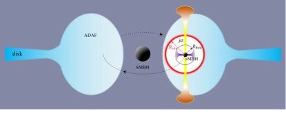
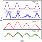
Figure 1: Left: An sMBH embedded in SMBH-ADAFs is orbiting around the central SMBH. The sMBH is accreting with Bondi rates from the SMBH-ADAF, but outflows from the sMBH-ADAFs drive the formation of a cavity and quench the accretion. Such an accretion-feedback system exhibits quasi-periodic behaviors, showing quasi-periodic flickerings from relativistic jets produced through the Blandford-Znajek (BZ) mechanism of the sMBH-ADAF. Emissions of the jet constitute spectral energy distributions additional to the SMBH-ADAF. The jet may be partially choked by the SMBH-ADAF, giving rise to sub-relativistic wisps from the SMBH-ADAF. The accumulating sMBH-outflows will trigger the viscosity instability of the SMBH-ADAF resulting in flares following a series of flickerings. The present model can explain the NIR quasi-periodic flickerings and flares of Sgr A$\!{}^{*}$ . Right: Illustrated classifications of light curves. Type-A shows that flares/flickerings are superposed on a stationary state whereas type-B shows an upon-down mode. Flickerings are thin lines and flares are thick lines.

2 The model

Figure 1 shows the model of the present AMS. An sMBH (the secondary BH as one satellite of the SMBH) is orbiting around the central SMBH (the primary) inside the ADAF. We assume a circular orbit in this binary black hole system. Parameters with the subscripts of “s” and “p” are referred to as those of the secondary and the primary. Their dimensionless accretion rates are defined by $\dot{\mathscr{M}}_{\rm p,s}=\dot{M}_{\rm p,s}/\dot{M}_{\rm Edd}^{\rm p,s}$, where $\dot{M}_{\rm p,s}$ are the accretion rates, $\dot{M}_{\rm Edd}^{\rm p,s}=L_{\rm Edd}^{\rm p,s}c^{-2}$ is their corresponding limit rate in light of the Eddington luminosity $L_{\rm Edd}^{\rm p,s}=4\pi GM_{\rm p,s}m_{\rm p}c/\sigma_{\rm T}$, where $G$ is the gravitational constant, $c$ is the speed of light, $m_{\rm p}$ is the proton mass, and $\sigma_{\rm T}$ is the Thomson cross-section. When $\dot{\mathscr{M}}$ is much less than the unity, the accretion flows are supported by the ion pressure of the plasma with two temperatures because cooling is so inefficient that most of the released energies are not able to radiate away. This results in that the accretion flows are very hot and are able to produce relativistic jet (Rees et al., 1982). This is the early version of ADAF. For simplicity, we use the self-similar solution of ADAF for the primary BH (Narayan & Yi, 1995), in which the half-thickness, density, and sound velocity are

$$\left\{\begin{array}[]{lll}H_{\rm p}&=&1.2\times 10^{12}\,M_{6}r_{1}\,{\rm cm},\\ n_{\rm e}&=&9.3\times 10^{9}\,\alpha_{0.1}^{-1}M_{6}^{-1}\dot{\mathscr{M}}_{{\rm p},\bar{3}}r_{1}^{-3/2}\,{\rm cm^{-3}},\\ c_{\rm s,p}&=&5.0\times 10^{9}\,r_{1}^{-1/2}\,{\rm cm\,s^{-1}},\\ v_{\rm r}&=&3.9\times 10^{8}\,\alpha_{0.1}r_{1}^{-1/2}\,{\rm cm\,s^{-1}},\end{array}\right.$$ (1)

where $\alpha_{0.1}=\alpha/0.1$ is the viscosity parameter (Shakura & Sunyaev, 1973), $r_{1}=R_{\bullet}/10R_{\rm g}$ is the radius of the disk from the SMBH, and $R_{\rm g}=GM_{\rm p}/c^{2}$ is the gravitational radius, $\dot{\mathscr{M}}_{\rm p,\bar{3}}=\dot{\mathscr{M}}_{\rm p}/10^{-3}$, $M_{6}=M_{\rm p}/10^{6}M_{\odot}$ is the mass of the primary black hole. There are three constants of $c_{1,2,3}$ in the self-similar solution (Narayan & Yi, 1995). In the case of an advection fraction ($f_{\rm adv}=0.9$ and the adiabatic index of $\gamma=4/3$), we calculate the three constants of $c_{1,2,3}=(0.42,0.55,0.28)$ from their definitions in this paper. Though the self-similar solution is used here, it is in agreement with the numerical solutions of the global ADAF. The density given by Eq. (1) is consistent with Chandra X-ray observations of Sgr A$\!{}^{*}$ , where the column density $N_{\rm H}\approx 8.0\times 10^{22}\,{\rm cm^{-2}}$ at the center (Wang et al., 2013), which is consistent with the inward extrapolation of the gas density from the Bondi radius (Xu et al., 2006). The ADAF scattering optical depth is about $\tau_{\rm es}\approx 0.007$ at $10\,R_{\rm g}$ in the vertical direction for these typical values given by Eq. (1), leading to different situations from the Shakura-Sunyaev disks, the jet developed by the sMBH could be not completely choked. The most prominent feature of the ADAF is the positive Bernoulli constant (defined as a sum of kinematic, thermal and potential energies of the ADAF gas), implying that outflows are developed by the advection mechanism since the accretion flows become gravitationally unbound by the SMBH (Narayan & Yi, 1994). Though the radiative efficiency of the ADAF is very low, the efficiency of outflows is quite high, resulting in strong feedback to the SMBH-ADAF and making a cavity around the sMBH.

For simplicity, we assume that the sMBH is trapped inside the SMBH-ADAF, and its Bondi accretion rates are given by

$$\dot{\mathscr{M}}_{\rm s}=\frac{\dot{M}_{\rm s}}{\dot{M}_{\rm Edd}}=\frac{4\pi G^{2}M_{\rm s}^{2}\rho_{\rm p}}{c_{s}^{3}\dot{M}_{\rm Edd}}=2.0\times 10^{-6}\,\alpha_{0.1}^{-1}\dot{\mathscr{M}}_{\rm p,\bar{3}}q_{\bar{5}},$$ (2)

where $M_{\rm s}$ is the mass of sMBH, $q_{\bar{5}}=q/10^{-5}$, $q=M_{\rm s}/M_{\rm p}$ is the mass ratio of the sMBH to the central SMBH, and $\rho_{\rm p}=n_{e}m_{\rm p}$ is the mass density of the SMBH-ADAF. This indicates that the sMBH is also the status of ADAF. It is interesting to note that the sMBH accretion rates are independent of its location. The Bondi radius of the sMBH

$$R_{\rm Bon}=\frac{GM_{\rm s}}{c_{\rm s,p}^{2}}=2.1\times 10^{8}\,\left(\frac{m_{1}}{4}\right)r_{1}\,{\rm cm},$$ (3)

where $m_{1}=M_{\rm s}/10\,M_{\odot}$ is the sMBH mass. $R_{\rm Bon}$ is much smaller than the Hill radius of $R_{\rm Hill}=(M_{\rm s}/M_{\rm p})^{1/3}R_{\bullet}\approx 3.2\times 10^{10}\,m_{1}^{1/3}M_{6}^{2/3}r_{1}\,{\rm cm}$, the SMBH tidal disruption of the AMS can be avoided. On the other hand, the outer radius (or the circularized radius) of the sMBH-ADAF can be estimated by angular momentum balance. The net specific angular momentum (AM) of the SMBH-ADAF is given by $\Delta\ell_{\rm p}=\Delta R\sqrt{GM_{\rm p}/R_{\bullet}}$, where $\Delta R$ is the width of the belt at $R$. The specific AM of the sMBH-ADAF can be approximated by $\Delta\ell_{\rm s}=\sqrt{X_{\rm out}GM_{\rm s}}$, where $X_{\rm out}$ is the outer radius of the sMBH-ADAF. Equating $\Delta\ell_{\rm p}=\Delta\ell_{\rm s}$ and $\Delta R\approx X_{\rm out}$, we have approximately $X_{\rm out}=\left(M_{\rm s}/M_{\rm p}\right)R_{\bullet}=1.5\times 10^{7}\,q_{\bar{5}}r_{1}M_{6}\,$cm, which is consistent with numerical simulations (e.g., Igumenshchev et al., 1999). The $X_{\rm out}$ is significantly smaller than the Bondi radius.

It should be noted that the orbiting sMBH suggested here is rotating with a supersonic velocity ($v_{\rm rot}\sim c/3$) at $10\,R_{\rm g}$. Shocks due to the motion could be produced to accelerate some electrons. Subsequently, non-thermal emissions of the electrons are thus radiated from this region. A similar case of the Bondi sphere of an isolated black hole supersonically moving in medium has been discussed by Wang & Loeb (2014), however, we will not discuss this potentially important point here. In this paper, only the case with an extremely low-$q$ system is considered. Such a system allows us to use the perturbation approximation to treat the influence of the sMBH on the SMBH-ADAF. Otherwise, we have to consider the inhomogeneity of the SMBH-ADAF caused by the sMBH feedback. We consider that the SMBH-ADAF is in a stationary state.

2.1 Cavity and flares

Since the progenitor of the sMBH should rotate very fast, the sMBH should also rotate fast and undergo two processes to generate influence on the SMBH-ADAF. First, energetic outflows with a power of $L_{\rm out}=\eta_{\rm out}\dot{M}_{\rm s}c^{2}$ are produced since the Bernoulli constant is positive, where $\eta_{\rm out}$ is the conversion efficiency of channeling gravitational energy into outflows. We note that $\eta_{\rm out}$ is much higher than the radiative efficiency of the ADAF and take $\eta_{\rm out}=0.1$ as a typical value in this paper. The higher $\eta_{\rm out}$ the more prominent effects of the sMBH on the SMBH-ADAF. Second, the Blandford-Znajek processes (BZ: Blandford & Znajek, 1977) form bi-polar relativistic jets. The outflows from sMBH-ADAF heat gas within the Bondi radius are efficiently clearing the gas in a timescale of $\Delta t_{\rm Bon}=\Delta E_{\rm Bon}/L_{\rm out}$, where $\Delta E_{\rm Bon}=GM_{\rm s}\Delta M_{\rm Bon}/R_{\rm Bon}$ is the gravitational energy of the gas, $\Delta M_{\rm Bon}\approx\frac{4\pi}{3}R_{\rm Bon}^{3}n_{e}m_{\rm p}$ is the gas mass within $R_{\rm Bon}$. For $n_{e}=10^{10}\,{\rm cm^{-3}}$, we have $t_{\rm Bon}\sim 0.017\,$s, and this demonstrates the sMBH-outflows have efficient feedback to form a cavity in the SMBH-ADAF. On the other hand, the smearing timescale of the Bondi cavity is approximately $R_{\rm Bon}/\alpha c_{\rm s}\sim 10^{-3}\,$s. In the Appendix, we list the other two classes of cavity formation. They have timescales much longer than $t_{\rm Bon}$, but significantly shorter than the flickerings and flares in Sgr A$\!{}^{*}$ . Moreover, the cooling timescale of local SMBH-ADAF is much longer than these cases. It can be regarded as a successive series of these events that creat a cavity as described below.

Outflows from the sMBH-ADAF will significantly affect the local structures of the SMBH-ADAF, generating a cavity with a radius of $R_{\rm cav}$, provided that the outflow kinetic energies exceed the local dissipation rates of gravitational energy of the SMBH-ADAF. This condition can be expressed as

$$L_{\rm out}\,{\color[rgb]{0,0,1}\gtrsim}\,\frac{4\pi}{3}R_{\rm cav}^{3}\varepsilon_{+},$$ (4)

where $\varepsilon_{+}\approx Q_{+}/H_{\rm p}$ is the volume dissipation rates of the SMBH-ADAF, $Q_{+}=3GM_{\rm p}\dot{M}_{\rm p}/8\pi R_{\bullet}^{3}$ is surface rates (Frank et al., 2002). Here, we neglect the factor of the inner boundary condition of accretion disks. We would like to point out the implications of Eq. (4), i.e., the outflow energies are the extra source of the SMBH-ADAF as type A variability shown in Fig. 1. In the following discussions, we take the equal form of inequality (4), and some results are the upper and lower limits for a given $L_{\rm out}$, for instance, $R_{\rm cav}$ in Eq. (6) and $\Delta t_{\rm cav}$ in (7), respectively. The cavity can be made by the work done within a time interval $\Delta t_{\rm cav}$ through the outflow-driven expansion of the heated part

$$L_{\rm out}\Delta t_{\rm cav}=\frac{4\pi}{3}R_{\rm cav}^{3}P_{\rm gas},$$ (5)

where $P_{\rm gas}=\rho_{\rm p}c_{\rm s}^{2}$ is the gas pressure of the SMBH-ADAF. Actually, Eq. (5) shares the same meaning of the work done $P\Delta V$ of AGN feedback in galaxy cluster (e.g., McNamara & Nulsen, 2007; Fabian, 2012). The ram pressure of the sMBH-outflows impedes the inflows outside the cavity through the balance with the surrounding medium, namely $L_{\rm out}/v_{\rm out}=4\pi R_{\rm cav}^{2}P_{\rm gas}$. We find that this condition holds as long as the outflows have a Mach number of ${\cal M}=v_{\rm out}/c_{\rm s}\geq 1$. Eq. (5) describes the working process of cavity formation, and is independent of (4). In the Appendix, we discuss the other two possibilities of cavity formation and find that they naturally satisfy the conditions (Eq. 4 and 5) employed here. During the cavity formation, we approximate the gas pressure as a constant. From this energy budget, we can derive the cavity radius

$$R_{\rm cav}=\left(\frac{3L_{\rm out}H}{4\pi Q_{+}}\right)^{1/3}=1.9\times 10^{10}\,\eta_{\rm 0.1}^{1/3}\alpha_{0.1}^{-1/3}r_{1}^{4/3}q_{\bar{5}}^{2/3}\left(\frac{M_{6}}{4}\right)\,{\rm cm},$$ (6)

and the time for cavity formation

$$\Delta t_{\rm cav}=\frac{HP_{\rm gas}}{Q_{+}}=45.9\,\alpha_{0.1}^{-1}r_{1}^{3/2}\left(\frac{M_{6}}{4}\right)\,{\rm min},$$ (7)

where $\eta_{0.1}=\eta_{\rm out}/0.1$. $R_{\rm cav}$ is comparable to the Hill radius, but is still much smaller than the half-thickness of the SMBH-ADAF. In the case of the SMBH-ADAF, $R_{\rm cav}$ is independent of the accretion rates of the SMBH-ADAF, but dependent of the location and mass of the sMBH, and the SMBH mass. Since $R_{\rm cav}\gg R_{\rm Bon}$, the sMBH will stop accretion in the timescale of the cavity formation. It is very interesting to note that the formation timescale is independent of the sMBH and its outflows but sensitive to its location radius and the SMBH mass. This offers an opportunity to measure the viscosity as the hardest parameter of accretion macro-physics if the location, sMBH mass, and flickering periods are fixed in the future (after detections of mHz gravitational waves). Actually, this $\Delta t_{\rm cav}$ is just the thermal instability timescale of $t_{\rm therm}=\Sigma c_{\rm s}^{2}/Q_{+}$ (e.g., Frank et al., 2002). We get this from the energy budget avoiding details of the expansion dynamics. Simultaneously, we should note that the BZ process generates relativistic ejecta during $\Delta t_{\rm cav}$. This produces flickerings as a result of the quenched Bondi accretion of the sMBH-outflows.

On the other hand, this cavity could be slacked down by the dynamical interaction or turbulence after the cessation of outflows. This rejuvenates the Bondi accretion of the sMBH. For a simple estimation, we can estimate the timescale of a rejuvenation

$$\Delta t_{\rm rej}=\frac{R_{\rm cav}}{v_{\rm tur}}=37.9\,\eta_{0.1}^{1/3}\alpha_{0.1}^{-4/3}q_{\bar{5}}^{2/3}r_{1}^{11/6}\left(\frac{M_{6}}{4}\right)\,{\rm s},$$ (8)

where $v_{\rm tur}=\alpha c_{\rm s}$ is the turbulence velocity, which is much shorter than $\Delta t_{\rm cav}$. The cavity is then destroyed by the turbulence of the cavity developed by the interaction between the outflows and the SMBH-ADAF. It is therefore expected that the cavity appears periodically with a timescale of $\Delta t_{\rm cav}+\Delta t_{\rm rej}\approx\Delta t_{\rm cav}$. A flickering lasts for $\Delta t_{\rm cav}$. It is very interesting to note that $\Delta t_{\rm cav}$ only sensitively depends on the location of the sMBH given the binary masses. From the observational side, the flickering period can be used to estimate the location. In practice, if the density of the SMBH-ADAF could be inhomogeneous, the flickering timescale could vary at different epochs. On the averaged behaviors, the sMBH undergoes quasi-periodic activities appearing as quasi-periodic flickerings. This is a unique feature of the AMS inside SMBH-ADAFs.

The sMBH is undergoing episodic Bondi accretion, but the cavity continually grows with time since the SMBH-ADAF is cooling much slower than the outflow-driven heating of the sMBH-ADAF. Therefore, the cavity density decreases, but its temperature and radius increase with time. Cooling processes inside the SMBH-ADAF involves bremsstrahlung (proton-electron and electron-electron collisions), synchrotron radiation and inverse Compton scattering (IC) (e.g., Narayan & Yi, 1995). Magnetic fields are usually estimated by the magnetization factor $\beta$, which is defined by $P_{\rm gas}=\beta(P_{\rm gas}+P_{\rm mag})$, where $P_{\rm mag}=B^{2}/8\pi$ is the magnetic pressure and $B$ is magnetic field. For the case of $\beta=0.5$, $n_{e}=10^{10}\,{\rm cm^{-3}}$ and $T_{\rm e}=10^{9}\,$K, we obtain the total emissivity of $\epsilon_{\rm tot}\approx\chi\,\epsilon_{\rm ff}$ and $\chi\approx 28$ (this can also be justified by comparing the NIR and hard X-ray peaks of ADAF SED as shown in Figure 2), where $\epsilon_{\rm ff}$ is the free-free emissivity. The cooling factor $\chi$ depends on the density, temperature and magnetization factor $\beta$. The cooling timescale of the shocked gas

$$\Delta t_{\rm cool}=\frac{3}{2}\frac{n_{\rm e}kT_{\rm s}}{\epsilon_{\rm tot}}\approx 5.6\,\chi_{0}^{-1}T_{9}^{1/2}n_{10}^{-1}\,{\rm hour},$$ (9)

where $\chi_{0}=\chi/28$, $n_{10}=n_{e}/10^{10}\,{\rm cm^{-3}}$, $k$ is the Boltzmann constant and $T_{9}=T_{\rm s}/10^{9}\,$K is the temperature of the shocked SMBH-ADAF. Since $\Delta t_{\rm cool}\gg\Delta t_{\rm cav}$, the SMBH-ADAF gas will be continuously heated by the sMBH-ADAF outflows, and the cavity grows with time. When it reaches the cooling timescale, the sMBH outflow accumulates power enough to produce a flare with a cavity radius

$$R_{\rm flare}\approx\left(\frac{3L_{\rm out}\Delta t_{\rm cool}}{4\pi P_{\rm gas}}\right)^{1/3}=3.7\times 10^{10}\,\eta_{0.1}^{1/3}\chi_{0}^{-1/3}T_{9}^{1/6}n_{10}^{-1/3}r_{1}^{5/6}q_{\bar{5}}^{2/3}\left(\frac{M_{6}}{4}\right)^{2/3}\,{\rm cm},$$ (10)

from Eq.(5), which is still much smaller than the thickness of the SMBH ADAF. The viscous instability of the SMBH-ADAF is developing in a timescale of $\Delta t_{\rm vis}\approx\alpha^{-1}(H/R_{\bullet})^{-2}t_{\rm\phi}$, where $t_{\phi}$ is the orbit period (e.g., Frank et al., 2002). For typical values and $H/R_{\bullet}\sim 1$, we have $\Delta t_{\rm vis}\approx 11.0\,\alpha_{0.1}^{-1}(M_{6}/4)r_{1}^{3/2}\,$hour, which is comparable with the cooling timescale. Therefore, the viscous instability will be unavoidably triggered by the accumulated energies of the sMBH-ADAF outflows. A flare releases the total energies of

$$E_{\rm flare}\approx\Delta t_{\rm flare}Q_{+}\left(\pi R_{\rm flare}^{2}\right)\approx 1.5\times 10^{40}\,\eta_{0.1}^{2/3}\chi_{0}^{-5/3}T_{9}^{5/6}n_{10}^{-5/3}r_{1}^{-4/3}\dot{\mathscr{M}}_{\rm p,\bar{3}}q_{\bar{5}}^{4/3}\left(\frac{M_{6}}{4}\right)^{1/3}\,{\rm erg},$$ (11)

where $\Delta t_{\rm flare}=\min(\Delta t_{\rm vis},\Delta t_{\rm cool})$ and we take $\Delta t_{\rm flare}=\Delta t_{\rm cool}$ here for a simple treament. A flare is rising with $\Delta t_{\rm flare}$, and decaying with $\Delta t_{\rm cool}$. The present model predicts that flares happen at a timescale of a few hours ($\Delta t_{\rm flare}$), and a few flares per day. However, the quiescent phase ($\Delta t_{\rm quiet}$) is complicated by the recovery of the flaring cavity of the SMBH-ADAF, which is controlled mainly by local cooling, viscosity-driven infalling gas of the local flows and viscosity dissipations of the gravitational energies. Flares are not periodic because of uncertainties of $\Delta t_{\rm quiet}$. This unique feature can be used to test the flickering origins (e.g., magnetic reconnection model). As we can see, this is in agreement with the observed flares in Sgr A$\!{}^{*}$ . For a flare state, the recovery of the SMBH-ADAF returning to its thermal equilibrium depends on joint processes of cooling and dynamical mixing, rather than a single process. Perturbation approximation is not valid in the state.

We would like to emphasize that the current treatments consider the sMBH activity as a perturbation. The validity of this approximation can be guaranteed provided that the expansion velocity of the cavity formation is sub-relativistic. When the mass ratio is large enough, the formation of a cavity will be different from the present. In such a case, the tidal torque of the sMBH-SMBH binary system is strong enough to engulf the SMBH-ADAF. This is very similar to the case of exoplanet formation. The accretion rates of the sMBH are much lower than Eq. (2) since the SMBH-ADAF density should be replaced by the density inside the gulf, however, it still significantly radiates for observations (since sMBH is large).

2.2 Quasi-periodic flickerings

Except for outflows from the sMBH-ADAF, relativistic ejecta would be developed by the BZ mechanism through extracting spin energy of the sMBH if it is rotating fast enough (Blandford & Znajek, 1977). Given a BH with spin AM ${\cal J}_{\bullet}$, the pumping power is given (Ghosh & Abramowicz, 1997; Macdonald & Thorne, 1982)

$$L_{\rm BZ}=\left(\frac{1}{32}\right)\omega_{\rm F}^{2}B_{\perp}^{2}R_{\rm h}^{2}c\left(\frac{{\cal J}_{\bullet}}{{\cal J}_{\rm max}}\right)^{2},$$ (12)

where $B_{\perp}$ is magnetic field $B$ normal to the horizon at $R_{\rm h}$, ${\cal J}_{\rm max}$ is the maximum of the spin AM, $\omega_{\rm F}=\Omega_{\rm F}(\Omega_{\rm h}-\Omega_{\rm F})/\Omega_{\rm h}^{2}$ is the factor describing relative angular velocity of magnetic field to the BH ($\Omega_{\rm h}$). Large scale magnetic field of the sMBH-ADAF, $B_{\perp}=B_{\rm disk}(H/r_{\bullet})^{1/2}$, $r_{\bullet}$ is the radius of the sMBH disk, which is formed by the fast radial motion (Livio et al., 2003; Cao, 2011), will be involved to form a jet, where $B_{\rm disk}$ is the azimuthal magnetic fields generated by the dynamo viscosity. Generally, geometrically thin disks $(H/r_{\bullet}\sim 10^{-2}-10^{-3})$ are not able to produce relativistic jets because of $B_{\perp}\ll B_{\rm disk}$. It should be noted that the sMBH-ADAF has much stronger $B_{\rm disk}$ than that of the SMBH-ADAF, which can be justified by Eq.(2.15) in Narayan & Yi (1995). For an optically thin ADAF, Armitage & Natarajan (1999) calculated the BZ power

$$L_{\rm BZ}\approx\frac{\sqrt{14}}{192}j_{\bullet}^{2}\dot{M}_{\rm s}c^{2}=1.92\times 10^{32}\,\alpha_{0.1}^{-1}j_{\bullet}^{2}\dot{\mathscr{M}}_{\rm p,\bar{3}}q_{\bar{5}}^{2}\left(\frac{M_{6}}{4}\right)\,{{\rm erg\,s^{-1}}},$$ (13)

where $j_{\bullet}={\cal J}_{\bullet}/{\cal J}_{\rm max}$, and we use the Bondi accretion rates (Eq. 2). Here, we take accretion rates of the sMBH during the interval of $\Delta t_{\rm cav}$ as a constant as an averaged one given by Eq. (2). Temporal profiles of the $L_{\rm BZ}$ depend on the evolution of density and temperature of the cavity, we will investigate this issue in the future.

The observational appearance of the BZ power release depends on two classes of factors: 1) the proceeding of the cavity formation driven by episodic accretion onto sMBH and 2) the dynamical interaction between the jet and the SMBH-ADAF, both of which determine the temporal profiles of the flickerings. These temporal processes make it very difficult to estimate the time-dependent Lorentz factor of the jets. Considering the difficulties in this paper, we consider two possible outcomes for the relativistic ejecta: 1) they are partially choked and exhibit sub-relativistic wisps after emerging; 2) they can penetrate the entire SMBH-ADAF resulting in the appearance of superluminal blobs. Without details of the jet dynamics, a flickering apparently appears when a jet can penetrate the SMBH-ADAF through a length of the ADAF and the Lorentz factor reaches

$$\Gamma\approx\frac{L_{\rm BZ}\Delta t_{\rm cav}}{\Delta M_{\rm j}c^{2}}\approx 8.5\,\alpha_{0.1}^{-1}x_{\rm j,1}^{-2}j_{\bullet}^{2}r_{1}^{2}\left(\frac{\ell_{j}}{H_{\rm p}/3}\right)^{-1},$$ (14)

where $\Delta M_{\rm j}=\pi X_{\rm b}^{2}\ell_{\rm j}n_{\rm e}m_{\rm p}$ is the mass of the jet, $x_{\rm j,1}=X_{\rm b}/10r_{\rm g}$ is the jet radius obtained from the analytical solution of the BZ process (e.g., Chen & Zhang, 2021), $r_{\rm g}$ is the gravitational radius of the sMBH, and $\ell_{\rm j}$ is its length. This is the average Lorentz factor of the jet, which is similar to that of radio-loud AGNs (Ghisellini et al., 1993). After the Lorentz factor falls below a critical one, the flickering disappears (since the Doppler boosting greatly weakens). Moreover, beyond this length, the jet experiences significant deceleration. Considering observational evidence of sub-relativistic ejecta from nuclear regions of the Galactic center (e.g., Rauch et al., 2016) and other low-luminosity AGNs (Middelberg et al., 2004), we choose case 1) that this jet is slowed down at $H_{\rm p}/3$ from relativistic states to sub-relativistic ones. The bulk Lorentz factor of the jet is similar to that of blazars (Ghisellini et al., 1993). It should be noted that the Lorentz factor is fully independent of the sMBH because both $L_{\rm BZ}$ and $\Delta M_{\rm j}$ are proportional to the square of the sMBH masses. From Eq.(14), we know the choked length is a significant fraction of the thickness of the SMBH-ADAF. The appearance of the jet strongly depends on the location of the sMBH as the result of SMBH-ADAF density. If the sMBH is located at around $20\,R_{\rm g}$ or so, the jet is capable of penetrating the entire SMBH-ADAF, showing superluminal motions of blobs. Considering the Doppler boosting effects, we have the observed luminosity of the jet inside the ADAF

$$L_{\rm jet}=L_{\rm BZ}{\cal D}^{4}=1.92\times 10^{36}\,\alpha_{0.1}^{-1}j_{\bullet}^{2}{\cal D}_{10}^{4}\dot{\mathscr{M}}_{\rm p,\bar{3}}q_{\bar{5}}^{2}\left(\frac{M_{6}}{4}\right)\,{{\rm erg\,s^{-1}}},$$ (15)

where ${\cal D}_{10}={\cal D}/10$, ${\cal D}=1/\Gamma(1-\beta_{\rm j}\cos\theta)$ is the Doppler factor, $\Gamma=1/\left(1-\beta_{\rm j}^{2}\right)^{1/2}$ is the Lorentz factor, $\beta_{\rm j}=v_{\rm j}/c$ is the jet velocity, and $\cos\theta$ is the cosine of the viewing angle. Here we take $\theta=5.7^{\circ}$ and $\Gamma=8.5$ for ${\cal D}=10$. We note that the SMBH-ADAF is optically thin ($\tau_{\rm es}\sim 0.008\ll 1$), which allows observers to see the emissions from the relativistic part of the choked jets. The choked part of the jet becomes ejecta, which carries the rest of the BZ power and can emerge with a sub-relativistic velocity of

$$\frac{v_{\rm eje}}{c}\approx\left(\frac{\xi L_{\rm BZ}\Delta t_{\rm cav}}{\Delta M_{\rm j}c^{2}}\right)^{1/2}=0.53\,\xi_{0.1}^{1/2}\alpha_{0.1}^{-1/2}j_{\bullet}x_{\rm j,1}^{-1}r_{1}\left(\frac{\ell_{\rm j}}{H_{\rm p}}\right)^{-1/2},$$ (16)

where $\xi_{0.1}=\xi/0.1$ is the fraction of the BZ power remaining after the jet radiates its most part of the BZ power. This is consistent with the wisps in Sgr A$\!{}^{*}$ observed by Rauch et al. (2016). If the relativistic ejecta is entirely choked, the emissions could be too faint to detect. In such a case, no flickering appears.

As a result of the continual heating of sMBH-outflows, the accumulated energies give rise to a flare. Therefore the number of flickerings can be estimated by considering the cooling and cavity timescales before a flare happens in the presence of the instability of the SMBH-ADAF (the regions with a radius of $R_{\bullet}\sim H_{\rm p}$ described by Eq.10). It follows from

$$N_{\rm flick}=\frac{\Delta t_{\rm cool}}{\Delta t_{\rm cav}}\approx 7.4\,\left(\frac{\Delta t_{\rm cool}}{5.6\,{\rm hour}}\right)\left(\frac{\Delta t_{\rm cav}}{45.9\,{\rm min}}\right)^{-1}.$$ (17)

This indicates that flares always appear after about a couple of flickerings. This is an important feature to observationally test the present model. Indeed, this is consistent with observations of Sgr A$\!{}^{*}$ (see the Spitzer data of Boyce et al., 2022).

The $L_{\rm BZ}$ (Eq. 13) is converted into the non-thermal emissions from the relativistic jet. Internal shocks are formed due to successive ejecta from the sMBH-ADAF whereas external shocks are formed through the collisions between the jet and the SMBH-ADAF. This process is similar to GRBs (e.g., Mészáros, 2002). Moreover, the jet is undergoing mass-loading processes when it penetrates through the SMBH-ADAF. The temporal profiles of flickerings, as discussed previously, depend on both the Bondi accretion processes and the propagation of the relativistic jet inside the SMBH-ADAF. Details of the temporal profiles of the flickerings can be further understood by numerical simulations. We would like to point out the diversity of the sMBH-driven phenomena. In the high-$\dot{\mathscr{M}}$ SMBH-ADAFs, the jet is seriously choked so that the Doppler boosting effects are too faint to see the flickerings, however, the sMBH-outflows can still trigger flares through viscous instability.

2.3 SED of the jet

In order to calculate the SED from the relativistic jet, we have to know the magnetic fields and energy distributions of non-thermal electrons. One-zone model is the simplest, in which non-thermal electrons, magnetic fields, and bulk Lorentz factor of the jet are homogenous and is often employed for the canonic SED of blazars (e.g., Inoue & Takahara, 1995). In the current case of sMBH-ADAF, the magnetic fields are so strong (than that of blazars) that SEDs generated by this model have too high-frequency cutoff even in the near-infrared bands (see Figure 3 for smaller index $m$). Therefore, we employ a simplified version of the inhomogeneous model of jets (Ghisellini et al., 1985; Georganopoulos & Marscher, 1998). Since both geometries of the jet and its magnetic fields are poorly understood, we consider a simple cone of the jet and its cross-sectional radius increases with height ($z_{\rm j}$) as $X_{\rm j}=X_{0}\left(z_{\rm j}/{z_{0}}\right)^{m}$, where $X_{0}$ is the jet radius at the base $z_{0}$ and index $m$ describes the geometry. In light of the self-similar solution (e.g., Narayan & Yi, 1995)

$$B_{\rm disk}=2.9\times 10^{4}\,\alpha_{0.1}^{-1}(1-\beta_{\rm s})^{1/2}\dot{\mathscr{M}}_{\rm p,\bar{3}}^{1/2}x_{1}^{-5/4}\left(\frac{M_{6}}{4}\right)^{-1/2}\,{\rm G},$$ (18)

where $\beta_{\rm s}$ is the magnetization parameter of the sMBH-ADAF, $x_{1}=X_{0}/10\,r_{\rm g}$ is the radius of the sMBH-ADAF. We assume that the poloidal magnetic fields of the jet (i.e., $B_{\perp}$ in Eq. 12) at its base follow the sMBH-ADAF, and have

$$B_{\rm j}=B_{\rm disk}\left(\frac{X_{\rm j}}{X_{0}}\right)^{-2}=B_{\rm disk}\left(\frac{z_{\rm j}}{z_{0}}\right)^{-2m},$$ (19)

based on a simple conservation of the magnetic fluxes. In this paper, we skip the details of electron acceleration, which involve many processes (formation and diffusions of shocks, energy gains and losses during the propagation of the jet through the SMBH-ADAF; see details in Blandford & Eichler, 1987). In the present paper, we assume a power law distribution of the electrons as

$$N_{\rm e}=N_{0}\gamma^{-s}\left(\frac{z_{\rm j}}{z_{0}}\right)^{-2m}\quad{\rm for}\,\,\gamma_{\rm min}\leq\gamma\leq\gamma_{\rm max},$$ (20)

where $\gamma$ is the Lorentz factor of non-thermal electrons, $\gamma_{\rm min,max}$ are the minimum and maximum, respectively, $s$ is the electron index, $N_{0}=(s-1)N_{\rm tot}/\gamma_{\rm min}^{1-s}\left[1-\left(\gamma_{\rm max}/\gamma_{\rm min}\right)^{1-s}\right]$, and $N_{\rm tot}$ is the number density of relativistic electrons. The factor $(z_{\rm j}/z_{0})^{-2m}$ results from the mass conservation in a continuous jet. We take $\gamma_{\rm min,max}$ as constants along the jet. When $m\rightarrow 0$, the present model tends to the one-zone model.

Emissions from the jet in its co-moving frame can be expressed by

$$L_{\nu}^{\rm Syn}=\int_{z_{0}}^{\ell_{\rm j}}\pi X_{\rm j}^{2}j_{\nu}^{\rm Syn}(z_{\rm j})\,dz_{\rm j};\quad{\rm and}\quad L_{\nu}^{\rm IC}=\int_{z_{0}}^{\ell_{\rm j}}\pi X_{\rm j}^{2}j_{\nu}^{\rm IC}(z_{\rm j})\,dz_{\rm j},$$ (21)

where $j^{\rm syn}_{\nu}$ and $j^{\rm IC}_{\nu}$ are the synchrotron and IC emissivities, respectively. We then transform these into the observer’s frame in order to compare with observations (e.g., Lind & Blandford, 1985). We neglect the synchrotron self-absorption since most photons are radiated from the sides of the jet and are beamed by the bulk motion of the jet, even if the optical depth is larger than unity along the jet direction. We neglect the pair production of the IC photons. The total number of non-thermal electrons $(N_{\rm tot})$ is constrained by $L_{\rm BZ}=\int_{z_{0}}^{\ell_{\rm j}}\pi X_{j}^{2}dz_{\rm j}\int_{\nu_{1}}^{\nu_{2}}\left(j^{\rm Syn}_{\nu}+j^{\rm IC}_{\nu}\right)d\nu$, where $\nu_{1}$ and $\nu_{2}$ are frequencies of the synchrotron radiation and IC. We use the standard formulations of synchrotron self-Compton (SSC) emissions and IC Blumenthal & Gould (1970) for the simple SED of the jet. We approximated it an isotropic radiation field. The ADAF is taken to be a point source with a luminosity $L_{\rm ADAF}$ and an averaged energy density of $u_{\rm ADAF}=L_{\rm ADAF}/4\pi R^{2}c$ at a distance $R$. In the co-moving frame, the relativistic jet receives an energy density of the SMBH-ADAF given by $U_{\rm ADAF}\approx\Gamma^{2}u_{\rm ADAF}$, which is the external source of seed photons (Sikora et al., 1994). We ignore external Compton scattering since $U_{\rm B}/U_{\rm ADAF}\sim 10^{6}$ holds in the current parameters of the jet. We omit all the formulations in this paper. Generally, there are two peaks of SEDs arising from synchrotron and IC, respectively.

We take $M_{6}=4.0$, $\dot{\mathscr{M}}_{\rm p,\bar{3}}=1$, $\alpha_{0.1}=1$. Following Narayan & Yi (1995) and Manmoto (2000), we take the electron heating coefficient $\delta=0.03$ in this paper though it may have large uncertainties (e.g., Yuan et al., 2003). We calculate the SMBH-ADAF SED for $\beta_{\rm p}=(0.99,0.5,0.35)$. Figure 2 shows the results. Generally, SEDs of the SMBH-ADAF are consistent with those of Manmoto (2000). The first peak of the SMBH-ADAF arises from synchrotron radiation of the Maxwellian distributions of hot electrons, and the peak shifts and powers vary with $\beta_{\rm p}$. Comptonization of the hot electrons results in the second peaks and bremsstrahlung contributes to the last peak with a cutoff related to the maximum temperatures of electrons.

For parameters of the jet, we take $x_{\rm j,1}=1$, $\ell_{\rm j}=H_{\rm p}/3$, $\Gamma=8.5$ and $\theta=5.6^{\circ}$. We fix the jet location at the radius of $x_{1}=1$. For a jet with $m=1/5$, the top of the jet $z_{\rm j,top}=\ell_{\rm j}\approx 10^{12}\,$cm, $\ell_{\rm j}/z_{0}\sim 10^{4}$, we have $X_{\rm j}\approx 7\,X_{0}$ and the magnetic fields decay by a factor of 50 along the jet height. The free parameters are $\gamma_{\rm min}$, $\gamma_{\rm max}$, $s$, $m$ and $\beta_{\rm s}$. We take $s=2.0$, $\gamma_{\rm min}=1$ and $\gamma_{\rm max}=10^{3}$ and $m=1/5$ for the theoretical SEDs. We adjust $\beta_{\rm s}$ in order to show the role of the magnetic fields in the jet SED. Since we keep the power of jets as a constant ($L_{\rm BZ}$), we adjust electron numbers for the dependence of the SED on magnetic fields, $\gamma_{\rm min,max}$, $\beta_{\rm s}$, $s$ and $m$. The synchrotron emissions shift towards lower frequencies with increases of $\beta_{\rm s}$ because $B$ decreases. As shown in Figure 2, the synchrotron emissions from the jet just supplement the deficits of the SEDs from SMBH-ADAFs depending on the maximum energies of electrons ($\gamma_{\rm max}$), in particular, contributing to infrared to soft X-ray bands. The SED of the jet shifts toward low frequency with decreases of $m$. This results from the fact that magnetic fields decrease along jet height with $m$. When $m$ tends to zero, the jet tends to the one-zone model.

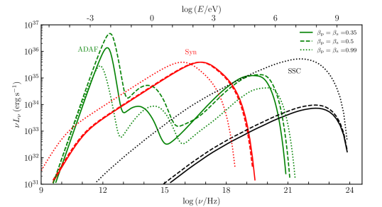
Figure 2: The overall spectral energy distributions of the SMBH-ADAF and the relativistic jets from the sMBH. The relativistic jet mainly contributes to the optical to soft X-ray bands. In these calculations, we take the same values of the magnetization parameter ($\beta_{\rm p,s}$) in the SMBH- and sMBH-ADAFs. See text for values of model parameters.

IC of synchrotron photons is significant compared with the power of the synchrotron emissions. It strongly depends on the magnetic fields of the sMBH-ADAF. In $\beta_{\rm p,s}=0.99$ case (weak magnetic field) as shown in Figure 2, the self-inverse Compton power is comparable with that of the synchrotron radiation. This significantly contributes to $\gamma$-ray bands but relies on $\gamma_{\rm max}$. With increases of magnetic fields ($\beta_{\rm s}$ decreases), the IC power decreases dramatically.

For a simple treatment, we take a constant bulk Lorentz factor of the jet in the present model. Dynamical interaction with the SMBH-ADAF will slow down the jet. A self-consistent treatment of this is necessary (e.g., Contopoulos & Kazanas, 1995) since the fully parameterized model of inhomogeneous jets could be useful to explore the SEDs of the sMBH-driven jets like in blazars (Georganopoulos & Marscher, 1998). Moreover, it is necessary to explore the time-dependent model of the relativistic jets for the temporal profiles of the light curves. This is left for future research. We would like to point out that the BZ process can also occur in the SMBH-ADAF if the SMBH is rotating fast enough. In such a context, emissions of the sMBH-ADAFs are overwhelmed by the SMBH-ADAFs. BL Lac objects and face-on radio galaxies (Fannaroff-Rilley I radio galaxies) are known to contain ADAFs which power relativistic jets (Sikora et al., 2007; Cao & Rawlings, 2004; Tadhunter, 2016). Actually, LLAGNs often show large radio-loudness (e.g., Ho, 2002) but lack powerful jets (e.g., Middelberg et al., 2004), implying that the SMBHs in most LLAGNs are non-rotating. There is no evidence that the BZ process works in SMBH-ADAF of Sgr A$\!{}^{*}$ , which only shows sub-relativistic wisps discovered by Rauch et al. (2016). If we apply Eq. (13) to Sgr A$\!{}^{*}$ , the BZ power will be around $10^{40}\,{\rm erg\,s^{-1}}$ if $j_{\bullet}\sim 1$, which is much more luminous than the observed the total emissions of Sgr A${}^{\!*}$. The central SMBH is thus expected to be very slowly spinning in Sgr A$\!{}^{*}$ . This is favored by the presence of two misaligned young stellar disks in light of the Lense–Thirring effects (Fragione & Loeb, 2022), though Event-Horizon-Telescope observations favor $j_{\bullet}\gtrsim 0.5$ (EHT Collaboration, 2022). Moreover, the observational fact that there are two counter-rotating young stellar disks within $30^{\prime\prime}$ regions (about 1 parsec) of the Galactic center identified by SINFONI IFU at the VLT (von Fellenberg et al., 2022) directly indicates random accretion onto the central SMBH, making the SMBH spin very low (Wang et al., 2009; Volonteri et al., 2013). Independent evidence for random accretion onto the central SMBH is provided by ALMA that two counter-rotating disks of gas in NGC 1068 have been found by Impellizzeri et al. (2019). Cancellations of the angular momentum of gas ($\lesssim 10\,$pc nuclear regions) finally drive extremely high accretion rates of the SMBH, which likely leads to an super-Eddington growth of the SMBH.

2.4 Gravitational waves

In this paper, an sMBH orbiting the central SMBH is an excellent EMRI (extreme mass ratio inspiral). We assume that the EMRI follows a circular orbit. This can be justified by the decaying of ellipticity due to radiations of gravitational waves (GWs). According to Peters (1964), we have the circularization timescale $t_{\rm E}=\left(d\ln e/dt\right)^{-1}$, where $e$ is the ellipticity of the initial orbit, if the GWs radiations govern the evolution of the EMRI orbit. A highly elliptical orbit of an EMRI will be circularized with $t_{\rm E}=\left(d\ln A/d\ln e\right)t_{\rm GW}\approx(1-10)\,t_{\rm GW}$ from an initial elliptical orbit of $e_{0}=0.9$ from $A=100\,R_{\rm g}$, where $A$ is the separation of the EMRI, $d\ln A/d\ln e=12\left[1+(73/24)e^{2}+(37/96)e^{4}\right]/19(1-e^{2})\left[1+(121/304)e^{2}\right]$. We expect that the sMBH undergoes rapid circularization of orbits and reaches a circular orbit at $A=10R_{\rm g}$. Their strain amplitudes and frequency of GWs from the EMRI are given by

$$h_{\rm s}=\left(\frac{128}{15}\right)^{1/2}\frac{\left(GM_{\rm c}\right)^{5/3}}{c^{4}d_{\rm L}}\left(\pi f\right)^{2/3}=7.6\times 10^{-17}\,d_{\rm 10kpc}^{-1}a_{1}^{-1}q_{\bar{5}}\left(\frac{M_{6}}{4}\right),$$ (22)

where $M_{\rm c}=\left(M_{\rm p}M_{\rm s}\right)^{3/5}\left(M_{\rm p}+M_{\rm s}\right)^{-1/5}=q^{3/5}(1+q)^{-1/5}M_{\rm p}$ is the chirping mass, and

$$f=\frac{2}{P_{\rm orb}}=0.5\,(1+q)^{-1/2}a_{1}^{-3/2}\left(\frac{M_{6}}{4}\right)^{-1}\,{\rm mHz},$$ (23)

where $P_{\rm orb}$ is the orbital periods, $d_{\rm 10kpc}=d_{\rm L}/10\,{\rm kpc}$ is the distance to observers, $a_{1}=A/10R_{\rm g}$ and $P_{\rm orb}$ is its orbital period. The GWs are in the bands of LISA (Laser Interferometer Space Antenna), and the other two space missions of Taiji (Hu & Wu, 2017) and Tianqin (Luo et al., 2016), whose thresholds ($h_{\rm s}\approx 10^{-20}$) are much lower than strains of the present EMRI. The decaying timescale of the circular orbit is (e.g., Peters, 1964)

$$t_{\rm GW}=\frac{A}{dA/dt}=\frac{5a^{4}}{64q(1+q)}\left(\frac{R_{\rm g}}{c}\right)\approx 48.8\,a_{1}^{4}q_{\bar{5}}^{-1}\left(\frac{M_{6}}{4}\right)\,{\rm yr},$$ (24)

which is a feasible timescale to witness an EMRI merger. We note that this timescale is very sensitive to the separation of the EMRI, and expect GRAVITY/VLTI to make a precise measurement of the orbit from the flares in Sgr A$\!{}^{*}$ .

In summary, an sMBH residing in the ADAF of the central SMBH has to undergo an episodic Bondi accretion governed by its strong feedback. A cavity is formed by the outflows from the accretion. During the accretion, a relativistic jet is formed by the BZ mechanism, showing quasi-periodic flickerings (jet emissions) from the sMBH-ADAF. Accumulations of the outflow energies will trigger the viscous instability of the SMBH-ADAF and generate a flare subsequently. Milli-Hz gravitational waves are radiated by the EMRI, which is strong for the detection of the designed space missions. Table 1 lists all the parameters involved in this model. Given a sMBH-SMBH system in the ADAF state, the temporal properties of the system can be predicted for quasi-periodic flickerings and flares.

Table 1: Parameters of the sMBH-SMBH system (EMRI)

Parameters		Meanings
Parameters describing the system given by the initial conditions
$M_{\rm p,s}$		Masses of the SMBH and sMBH, respectively; the mass ratio is defined by $q=M_{\rm s}/M_{\rm p}$
$\dot{\mathscr{M}}_{\rm p,s}$		Dimensionless accretion rates of the SMBH and sMBH in units of $L_{\rm Edd}/c^{2}$, respectively
$R_{\bullet}$		sMBH location radius at the SMBH-ADAF (or $A$: the separation between sMBH and SMBH)
Parameters of accretion physics
$\alpha_{\rm p,s}$		Viscous parameters of the SMBH and sMBH
$\beta_{\rm p,s}$		Magnetization parameters of the SMBH and sMBH
$\eta_{\rm out}$		Efficiency of outflows driven by sMBH-ADAF
Derived parameters of the system for observations of flickerings and flares
$R_{\rm cav}$		Radius of the cavity created by the SMBH-ADAF outflows
$\Delta t_{\rm cav}$		Formation timescale of the cavity as the quasi-periods of flickerings
$\Delta t_{\rm cool}$		Cooling timescale of the SMBH-ADAF as outburst timescales of flares
$R_{\rm flare}$		Radius of the cavity zones generating flares from the SMBH-ADAF
$L_{\rm BZ}$		Blandford-Znajek power of the sMBH
$j_{\bullet}$		Specific angular momentum of the sMBH
$\Gamma$		Lorentz factor of the relativistic jet developed by the sMBH-ADAF
$v_{\rm eje}$		Sub-relativistic velocity of the choked part of the relativistic jet
$N_{\rm flick}$		Numbers of flickerings triggering a flare
$h_{\rm s}$		Strains of the gravitational waves from the sMBH-SMBH binary system
$f$		Frequency of the gravitational waves
$t_{\rm GW}$		Timescales of orbital decays due to gravitational waves
Parameters of the relativistic jet (assumed in this paper)
$X_{\rm j}$		Cross-sectiobal radius of the jet; $X_{0}$ is the initial radius
$\ell_{\rm j}$		Length of the jet; $z_{0}$ is the initial height of the jet; $z_{\rm j}$ is jet height
$s$		Distribution index of non-thermal electrons of the relativistic jet ($\propto\gamma^{-s}$)
$m$		Geometric index of the cross-sectional radius of the jet versus its height ($X_{\rm j}\propto z_{\rm j}^{m}$)
$\gamma_{\rm min,max}$		Minimum and maximum Lorentz factors of non-thermal electrons

2.5 Discussions

In this paper, the AMS plays a role in perturbations of the SMBH-ADAF while the latter is in a relatively stationary state. Flickerings are a tiny fraction of the SMBH-ADAF radiation but the flares are stronger than the former. Therefore, light curves are expected to show as depicted by the right panel of Figure 1, where flares and flickerings are thus just superposed on a relatively stationary radiation flux. If the sMBH is non-rotating (or its rotation is not fast enough), flickerings disappear (the lower panel). We denote this type-A light curve, and type-A1 and type-A2 for the cases with and without flickerings, respectively. Actually, Sgr A$\!{}^{*}$ shows the type-A light curves, see Figure 1 in Boyce et al. (2022), NGC 4151 (see Figure 4 in Chen et al., 2023b), and NGC 5548 (see Figure 3 of Li et al., 2016).

For high-$q$ system, however, feedback of the sMBH accretion to the SMBH-ADAF is not a perturbation. Large zones of the SMBH-ADAF will be broken, and giant flares are expected from these high-$q$ systems. We hence anticipate an upon-down style of light curves. This denotes type-B light curves. Similar to type-A curves, type-B curves are distinguished as type-B1 and type-B2 with and without flickerings, respectively. Actually, Arakrian 120 has exhibited type-B light curves over the last 20 years (Li et al., 2019). Collections of low-$\dot{\mathscr{M}}$ AGN light curves can test this classification, but it needs homogeneous light curves spanning longer than 20-30 years. We emphasize that these classifications of light curves are only valid for the case that the central SMBHs have ADAFs, and the physics for SMBHs with high-$\dot{\mathscr{M}}$ should be reconsidered separately.

In the present study, we set the typical values of an AMS with a mass of $\sim 40M_{\odot}$ at $10\,R_{\rm g}$ around the central SMBHs of $4\times 10^{6}M_{\odot}$ for the Galactic Center. The resultant properties of the AMS depend on its mass, location and the SMBH-ADAF accretion rates. The BZ power is proportional to $M_{\rm s}^{2}$ (see Eq. 13). Fates of the relativistic jet depend on the SMBH-ADAF. It either penetrates the ADAF and shows superluminal motion outside the nucleus, or is partially choked by the ADAF giving rise to sub-relativistic ejecta from the nucleus (see Eq.16). If the BZ power is not strong enough compared with the SMBH-ADAF damp, flares still occur but without flickerings. Moreover, the sMBH has a Keplerian rotation velocity of $v_{\rm rot}\sim c/3$ at $R_{\bullet}\sim 9\,R_{\rm g}$, emissions from the jet developed by the sMBH-ADAF could be modulated by transverse Doppler boosting. Additionally, general relativistic effects should be employed for temporal profiles of flickerings.

Shocks formed by the dynamic interaction between sMBH-outflows and SMBH-ADAF can accelerate electrons and generate non-thermal emissions. As a simple estimation, the kinetic power of the shocks is around $L_{\rm out}\approx 8\times 10^{33}\,{\rm erg\,s^{-1}}$, and about 10% of $L_{\rm out}$ will be channelled into non-thermal electrons (e.g., Blandford & Eichler, 1987) and contribute to multiwavelength continuum. This component causes complicated behaviors of variabilities of the system. We remain this topic as a future issue.

We assume that the global SMBH-ADAF is stationary. It is then expected to exhibit quasi-periodicity of flickerings and flares from the system. However, the reality could be complicated. For example, $\dot{\mathscr{M}}_{\rm p}$ is a function of the radius of SMBH-ADAF (Blandford & Begelman, 1999), and due to clump accretion (Wang et al., 2012a), the periodicity of flickerings and flares dramatically decreases and even becomes random sometimes. For example, NGC 5548 shows preliminary periodicity in its long-term light curves with flickerings (Li et al., 2016), but the periodicity of flickerings is usually verily twinkled by showing 3-4 cycles.

Finally, we would like to point out the key tests of the present model. LISA detections around 2030 can more accurately determine the EMRI system for a concluding remark. Before the LISA era, GRAVITY+/VLTI observations of Sgr A$\!{}^{*}$ can provide more solid and accurate loci of NIR-flares from increasing observations to obtain the orbiting radius of flares, on which the merger timescale sensitively depends. The current error bars of the flare’s loci are still quite large (about $30-50\%$). Flickering numbers associated with flares are another feature of the EMRI system, and we anticipate acquiring more data for high statistics of the flares and flickerings.

3 Application to Sgr A$\!{}^{*}$ 

As a preliminary practice of the present model, we apply it to Sgr A$\!{}^{*}$ , which is the best-studied low-luminosity system. An early extensive review on this object can be found for general properties in Genzel et al. (2010). It has been extensively observed through multiwavelength campaigns during the last 20 years and shows a diversity of variability properties (see a brief summary of observations in Witzel et al., 2021; Boyce et al., 2022; von Fellenberg et al., 2023). The powerful astrometric measurements of GRAVITY/VLTI provide an exciting ring of locations of flares during the last four years. The ring is phenomenologically explained as a moving hot spot around the SMBH. It has a radius of $R_{\bullet}=8.9_{-1.3}^{+1.5}\,R_{\rm g}$ and is rotating with the azimuthal speed of near Keplerian motion (see also their Figure 7 in Gravity Collaboration, 2023a). A hot spot due to magnetic reconnection in the SMBH-ADAF has been suggested for flares in Sgr A$\!{}^{*}$ (see references subsequently cited), but an orbiting sMBH can explain the properties of flares and flickerings as an alternative model. Actually, the light curves show that flickerings and flares are superposed on relatively stationary fluxes (see Spitzer, Chandra light curves Boyce et al., 2022), implying that they are perturbations of the SMBH-ADAF. This indicates that Sgr A$\!{}^{*}$ should be classified as one type-A2 object.

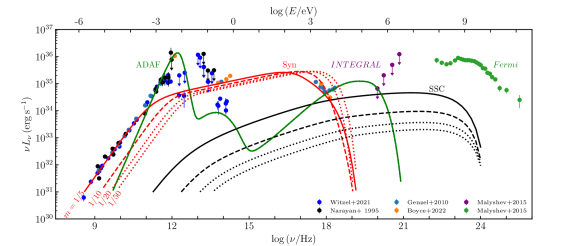
Figure 3: The overall spectral energy distribution of Sgr A$\!{}^{*}$ from radio to TeV bands. We get the accretion rates of the SMBH from the averaged SED. Curves are marked by the same color words. Syn: synchrotron radiation from the relativistic jet developed by the sMBH accretion. ADAF-EC: external IC of SMBH-ADAF photons. SSC: synchrotron self-Comptn scattering. Narayan & Yi (1995) collected early radio data (we omit these references). INTEGRAL and Fermi data are from Malyshev et al. (2015). When $m\rightarrow 0$, the inhomogeneous model becomes one-zone model.

3.1 Accretion rates

The SMBH mass is accurately measured $M_{\rm p}=4.3\times 10^{6}\,M_{\odot}$ (see the latest values given by Gravity Collaboration, 2022). The classical ADAF model was first applied to explain SED (from radio to hard X-rays) of Sgr A$\!{}^{*}$ (Narayan et al., 1995), which was revised by including fully general relativistic effects (e.g., Manmoto, 2000; Li et al., 2009). Figure 3 shows the global SED from radio to TeV bands. We use the classical ADAF model (e.g., Li et al., 2009) to get the accretion rates for discussions on the sMBH properties. $\gamma$-ray emissions through hot proton-proton collisions in the ADAFs have been suggested by Mahadevan et al. (2003), but it is only a small fraction of the total ADAF emissions (Oka & Manmoto, 2003) that is much below the Fermi observations as shown by Figure 3. For Sgr A$\!{}^{*}$ , there are only three free parameters in this model, accretion rates ($\dot{\mathscr{M}}$), viscosity ($\alpha$) and magnetization parameter ($\beta_{\rm p}$). We take the SMBH mass measured by GRAVITY (Gravity Collaboration, 2022), and fix the typical values of the magnetization parameter of $\beta=0.35$ and the viscosity of $\alpha=0.1$. We find $\dot{\mathscr{M}}_{\rm p}=10^{-3}$ for a global fitting (the green line for most points except for flaring points in Figure 3), which agrees with previous results of Manmoto (2000).

It has been also suggested that the X-ray flare emission is due to synchrotron radiation (Dodds-Eden et al., 2009; Barriére et al., 2014; Ponti et al., 2017) although it has been also interpreted as IC upscattered photons by the mildly relativistic, nonthermal electrons (Markoff et al., 2001; Yuan et al., 2003; Yusef-Zadeh et al., 2009; Ball et al., 2016). It is obvious that the Fermi $\gamma$-ray emissions (Chernyakova et al., 2011; Malyshev et al., 2015) are much beyond the scope of the SMBH-ADAF continuum emissions, but they have a luminosity of $10^{36}\,{\rm erg\,s^{-1}}$ from 100 MeV to 500 GeV. It has been suggested by Malyshev et al. (2015) that the Fermi-detected bump originates from IC by high-energy electrons in extensive regions, indicating an extra source of non-thermal emissions in Sgr A$\!{}^{*}$ (see the possibilities discussed in Cafardo & Nemmen, 2021). It is not our goal to extensively explore the delays among the multiwavelength variations, but we explain the major properties of flickerings and flares and suggest future tests of the present model.

3.2 Flares and quasi-periodic flickerings

NIR flares are more common on timescales of hours or so. X-ray flares often accompany NIR ones, but sometimes don’t (Boyce et al., 2022). Several kinds of models are suggested to explain multiwavelength variations, such as, the popular magnetic reconnection events (e.g., Dexter et al., 2020; Mellah et al., 2023), non-thermal electrons in a jet (Markoff et al., 2001; Yuan et al., 2003), sudden instabilities of the MHD disk (e.g., Chan et al., 2009), or other stochastic processes in the ADAFs (see more references listed by Boyce et al., 2022). The most interesting is that Genzel et al. (2003) discovered quasi-periodic flickerings of $\sim 17\,$min, which were superimposed to a flare in NIR bands during one epoch of 2002 (but see different results in other epochs of Do et al. 2009). X-rays of XMM-Newton observations show the similar periods (Aschenbach et al., 2004; Eckart et al., 2006). This quasi-periodic flickering (at 4$\mu$m) has been confirmed by the Spitzer observations (Boyce et al., 2022). It has been argued that the appearance of the flickering quasi-periodicity ($17\sim 40\,$min) depends on epochs (see a summary of the quasi-periodicity in Genzel et al., 2010) though Do et al. (2009) thought of the res-noise roles. The quasi-periodicity of flickerings has been suggested to arise from the quasi-periodic structure of plasma as hot spots (e.g., Dexter et al., 2020; Mellah et al., 2023; Aimar et al., 2023; Lin et al., 2023) or expanding hot spot (Michail et al., 2023). However, this kind of models involving magnetic reconnections should explain why the flares constantly happen at the same radius (namely, $\sim 9R_{\rm g}$) since the reconnections randomly happen somewhere inside the SMBH-ADAF. Second, one orbiting star as a pacemaker is suggested by Leibowitz (2021) for the periodicity of NIR and X-ray flares. A hidden black hole with a mass of $\sim 10^{4}M_{\odot}$ has been suggested by Naoz et al. (2020), however, the black hole with $\gtrsim 10^{3}M_{\odot}$ has been ruled out by precise measurements of S2 orbits (Gravity Collaboration, 2023b; Will et al., 2023). Recently, Gravity Collaboration (2023a) maps the loci of the flare’s locations during the last 4 years and finds that the loci are consistent with the Keplerian orbits at a distance of $\sim 9\,R_{\rm g}$ from the central SMBH well determined by the S2 star. For the magnetic reconnection model of the hot spots, the question of how to keep them in similar loci remains open. This new solid evidence supports a rigid body around the central SMBH. We suggest here an sMBH is orbiting around the SMBH in Sgr A$\!{}^{*}$ in charge of flares and quasi-periodic flickering.

For simplicity, we assume the sMBH spin axis to be perpendicular to the SMBH-ADAF equatorial plane. Since the quasi-periods are about $17-40$ min (we take the mean quasi-period is bout 30 min), we have the accretion rates of $\dot{\mathscr{M}}_{\rm s,\bar{6}}\approx 2.0$ from Eq. (2), $\dot{\mathscr{M}}_{\rm p,\bar{3}}=1.0$, $r_{1}=0.9$, and $M_{6}\approx 4.3$. We obtain the quasi-periods of $\Delta t_{\rm cav}\approx 42.1\,\alpha_{0.1}^{-1}$min from Eq. (7), which is in agreement with observed quasi-periods (Genzel et al., 2010) if $\alpha_{0.1}\approx 1.5\sim 2$ slightly fluctuates. Flares are generated with $\Delta t_{\rm vis}\approx 10.1\,$hour, which is well consistent with the observed, namely, there are a few flares per day. The SED of the jet is shown in Figure 3, where we take $s=2.6$, $\beta_{\rm s}=0.35$, $\gamma_{\rm min}=2.0$, $\gamma_{\rm max}=10^{3}$, $m=1/5,\,1/10,\,1/20,\,1/50$, respectively, for the 1-100 GHz bands, NIR bands and soft X-rays. The most significant effects are observed in the SED at low frequencies. The well-known 1-100 GHz emissions beyond the SMBH-ADAF, which are usually explained by a relativistic jet from the SMBH-ADAF lacking of choke effects (Markoff et al., 2001; Yuan et al., 2003; Yusef-Zadeh et al., 2009; Ball et al., 2016), can be reasonably explained by the present model. Ejecta from Sgr A$\!{}^{*}$ has been observed but it is sub-relativistic (Rauch et al., 2016). The present model is consistent with the ejecta. It should be mentioned that some parameters degenerate in fitting SED, for example, $\gamma_{\rm min}$, $m$ and $\beta_{\rm s}$. The most important thing is to identify this EMRI system at this stage, and we leave it for the future to make a self-consistent model for jet emissions. However, the Fermi SED cannot be explained by the present jet model. We agree that Fermi $\gamma$-ray emissions are from extensive regions since no evidence is found for $\gamma$-ray variability (e.g., Cafardo & Nemmen, 2021).

The simple model can, in principle, explain the major properties of the flares and quasi-periodic flickerings. We note that the extensive multiwavelength observations show complicated behaviors of variations, such as delays among radio, NIR and X-ray bands. Though some attempts have been made (e.g., Okuda et al., 2023), we will apply the present model to Sgr A$\!{}^{*}$ in more sophisticated treatments to explain variabilities and polarizations by including inner shocks and external shocks of the jet. Moreover, wisps with sub-relativistic velocity ($\sim 0.4\,$c) from Sgr A$\!{}^{*}$ have been discovered by Rauch et al. (2016), which could be the remnant, i.e., $\xi L_{\rm BZ}$, of the relativistic jets slowed down by interaction with surrounding medium from the sMBH-ADAF. Indeed, LLAGs often show sub-relativistic ejecta (e.g., Middelberg et al., 2004). A damped jet model will be discussed for this issue in a separate paper. A few points would be stressed as follows.

First, the non-thermal emissions from the relativistic jet can be, in practice, tested by a multiwavelength campaign of simultaneously monitoring Sgr A$\!{}^{*}$. In particular, the GHz radio and soft X-rays correlations (synchrotron emissions), and with Fermi $\gamma$-ray bands (external IC) are the keys to testing the present model of the sMBH. Hard X-rays may be mainly contributed by the SMBH-ADAF. Second, the emissions from the shocks formed by the outflows and SMBH-ADAF also contribute to emissions in some bands from radio to X-rays (even soft $\gamma$-rays). This makes the tests not so direct. Okuda et al. (2023) made an extensive analysis of the multiwavelength correlations, but they draw conclusions that the multiwavelength continuum has complicated originations. The correlations may depend on the states of Sgr A$\!{}^{*}$. Third, optical and UV bands are the key bands of testing SMBH-ADAF model, but it is impossible to have observations owing to the heavy extinctions of the Galactic center. Fortunately, INTEGRAL (The International $\gamma$-ray Laboratory: 15 keV-10 MeV) has a sensitivity ($\sim 2.85\times 10^{-6}\,{\rm ph\,s^{-1}\,cm^{-2}}$ with an exposure time of $10^{6}\,$s at 100 keV, see https://www.cosmos.esa.int/web/integral/instruments-ibis) higher than the IC scattering of SMBH-ADAF photons, and is promising to detect the emissions to test the present model. However, INTEGRAL is not able to spatially resolve the region of the Galactic Center so that only upper limits are given by Malyshev et al. (2015). As to Fermi observations, the present model is not able to produce enough $\gamma$-ray emissions to explain the data. We agree that these $\gamma$-rays are from extended regions or other compact objects in the Galactic Center (Cafardo & Nemmen, 2021).

3.3 mHz gravitational waves

If the $40M_{\odot}$ black hole is orbiting around the central SMBH, Sgr A$\!{}^{*}$ will be an excellent target of LISA detection (Babak et al., 2017). From Eq. (22), we find the strain amplitude $h_{\rm s}=1.4\times 10^{-17}$, which is very strong for LISA. The decaying timescale of the orbits is $t_{\rm GW}\approx 32.9_{-15.4}^{+28.4}\,$years for $q_{\bar{5}}=1$, $M_{6}=4.3$ and $a_{1}=0.9$ in light of the current error bars of the orbital radius ($A$) from GRAVITY. More data are needed from GRAVITY to determine $A$ better with higher statistics. The key test is from LISA to detect the strains and polarizations of the mHz gravitational waves from the EMRI and its orbital decays. See some detailed calculations of mHz gravitational waves from an EMRI, which can be found in Fang et al. (2019), Bondani et al. (2022) and Tahura et al. (2022). Considering the general relativistic effects, the Schartzshild procession of the sMBH is about $\Delta\phi\sim 6\pi R_{\rm g}/R_{\bullet}\approx 108^{\circ}\,r_{1}^{-1}$ per period for a circular orbit. Therefore, it is feasible for GRVAVITY+/VLTI to measure the procession and decay of the orbit (through loci of the flare’s location). Fully general relativistic treatments should be simultaneously done for both Schwartzschild procession and gravitational waves. Sgr A$\!{}^{*}$ is an excellent laboratory for general relativity through gravitational waves detected by LISA / Taiji / Tianqin, and orbits measured by GRAVITY+/VLTI.

4 Conclusions

We outline a model of the case of a stellar-mass black hole (sMBH) as one satellite of the SMBH embedded in the advection-dominated accretion flows (ADAFs). The Bondi accretion onto the sMBH drives the formation of a cavity through outflows and leads to quenching the accretion. A cavity is expected to quasi-periodically appear in the SMBH-ADAF, and accumulated energies of sMBH outflows during its growth will make flares through viscous instability. Relativistic jets are developed by the Blandford-Znajek mechanism if the sMBH is maximally rotating, and will significantly emit non-thermal radiations spanning from radio to $\gamma$-rays. The non-thermal emissions from the relativistic jet follow the episodic cavities as quasi-periodic flickerings. Such an Extreme Mass Ratio Inspiral (EMRI) is an excellent laboratory for milli-Hertz gravitational waves.

As a simple application of the present model, we explain the flares and quasi-periodic flickerings of Sgr A$\!{}^{*}$ within the framework of the present scenario. GRAVITY/VLTI maps of the locations of flares in Sgr A$\!{}^{*}$ consist of a ring, which supports the present model. The quasi-periodic flickerings are consistent with the flare’s location, and flares take place driven by accumulations of about 10 flickerings. The satellite black hole with $M_{\rm s}\approx 40M_{\odot}$ is favored from fitting the SED of Sgr A$\!{}^{*}$ spanning from radio to X-ray bands, where the relativistic jet is developed from the episodic sMBH-ADAF. The strain amplitudes of the mHz gravitational waves are about $10^{-17}$ and the sMBH will merge into the central SMBH in 30 years. More precise measurements of the sMBH orbits are expected as well as mHz GW detections of LISA / Taiji / Tianqin to reveal the presence of the sMBH.

Though we only provide formulations for an EMRI with a mass ratio of $10^{-5}$ around $10^{6}\,M_{\odot}$ SMBH, the present model is also applicable to $\gtrsim 10^{6}\,M_{\odot}$ system. Applications of the present scenario to other massive AGNs (e.g., Pyatunina et al., 2006) or 3C 390.3-like radio galaxies (Sergeev, 2020) will be carried out. For high-$q$ systems, such as $q\sim 10^{-2}$, the properties of the system will be different from the present descriptions, showing much larger cavities than the low-$q$ ones. In such a context, the EMRI system shows large amplitudes of flares i.e., an upon-down mode of variabilities, and flickerings appear/disappear depending on the sMBH spins.

Finally, we would like to point out the possibility that multiple sMBHs may simultaneously coexist and randomly distribute inside the SMBH-ADAF. Since the properties of sMBH cavities are sensitive to the locations and masses, flickerings and flares are superposed on each other. The quasi-periodicity of light curves arising from all of them may disappear but show random behaviors. In general, light curves of LLAGNs should be complicated if they contain multiple sMBHs.

Appendix A Other processes of cavity formation

In order to form a cavity, the sMBH-outflows should work to overcome possible barriers. First, the outflows work against the gravitational energy between the sMBH and the cavity gas. This means $\Delta E_{1}=GM_{\rm s}\Delta M_{\rm cav}/R_{\rm cav}$, where $\Delta M_{\rm cav}=\frac{4\pi}{3}R_{\rm cav}^{3}n_{\rm e}m_{\rm p}$. We have the timescale of cavity formation

$$\Delta t_{1}=31.1\,\eta_{0.1}^{-1/3}\alpha_{0.1}^{-2/3}r_{1}^{7/6}q_{\bar{5}}^{1/3}\left(\frac{M_{6}}{4}\right)\,{\rm s},$$ (A1)

where $\eta_{0.1}=\eta_{\rm out}/0.1$. Second, the outflows should overcome the SMBH binding energy, and $\Delta E_{2}=\Delta M_{\rm cav}(GM_{\rm p}/R_{\bullet}^{2})R_{\rm cav}$. The timescale is given by

$$\Delta t_{2}=31.9\,\eta_{0.1}^{1/3}\alpha_{0.1}^{-4/3}r_{1}^{11/6}q_{\bar{5}}^{2/3}\left(\frac{M_{6}}{4}\right)\,{\rm s}.$$ (A2)

The above estimations show that the outflows can easily make a cavity. Third, the outflows should work against the gas pressure of the SMBH-ADAF, that is $\Delta E_{3}=\frac{4\pi}{3}R_{\rm cav}^{3}P_{\rm gas}$ in the main text (e.g., McNamara & Nulsen, 2007; Fabian, 2012). Comparing the three cases, we find that the third case can make a much large cavity than the other two.

References

- Abbott et al. (2020) Abbott, R., Abbott, T. D., Abraham, S. et al. 2020, Phys. Rev. Lett., 125, 101102
- Ahnen et al. (2017) Ahnen, M. L., Ansoldi, S., Antonelli, L. A. et al. 2017, A&A, 601, 33
- Aimar et al. (2023) Aimar, N., Dmytriiev, A., Vincent, F. H., et al. 2023, A&A, 672, A62
- Armitage & Natarajan (1999) Armitage, P. J. & Natarajan, P. 1999, ApJ, 523, L7
- Aschenbach et al. (2004) Aschenbach, B., Grosso, N., Porquet, D., & Predehl, P. 2004, A&A, 417, 71
- Babak et al. (2017) Babak, S., Gair, J., Sesana, A. et al. 2017, arXiv:1703.09722
- Ball et al. (2016) Ball, D., Özel, F., Psaltis, D., & Chan, C.-K. 2016, ApJ, 826, 77
- Barriére et al. (2014) Barriére, N. M., Tomsick, J. A., Baganoff, F. K., et al. 2014, ApJ, 786, 46
- Bartos et al. (2017) Bartos, I., Kocsis, B., Haiman, Z., & Márka, S. 2017, ApJ, 835, 165
- Blandford & Begelman (1999) Blandford, R. & Begelman, M. L. 1999, MNRAS, 303, L1
- Bellovary et al. (2016) Bellovary, J. M., Low, M.-M.-M., McKernan, B., & Ford, K. E. S. 2016, ApJ, 819, L17
- Blandford & Eichler (1987) Blandford, R. & Eichler, D. 1987, Phys. Rep., 154, 1
- Blandford & Znajek (1977) Blandford, R. D., & Znajek, R. L. 1977, MNRAS, 179, 433
- Blumenthal & Gould (1970) Blumenthal, G. R. & Gould, R. J. 1970, RvMP, 42, 237
- Bondani et al. (2022) Bondani, S., Haardt, F., Sesana, A. et al. 2022, Phys. Rev. D, 106, 043015
- Boyce et al. (2022) Boyce, H., Haggard, D., Witzel, G. et al. 2022, ApJ, 931, 7
- Cafardo & Nemmen (2021) Cafardo, F. & Nemmen, R. 2021, ApJ, 918, 30
- Cao & Rawlings (2004) Cao, X. & Rawlings, S. 2004, MNRAS, 349, 1419
- Cao (2011) Cao, X. 2011, ApJ, 737, 74
- Chakraborty et al. (2021) Chakraborty, J., Kara, E., Masterson, M., et al. 2021, ApJ, 921, L40
- Chan et al. (2009) Chan, C.-K. et al. 2009, ApJ, 701, 521
- Chen et al. (2023a) Chen, K., Ren, J. & Dai, Z.-G. 2023, ApJ, 948, 136
- Chen et al. (2023b) Chen, Y.-J., Bao, D.-W., Zhai, S. et al. 2023, MNRAS, 520, 1807
- Chen & Zhang (2021) Chen, L. & Zhang, B. 2021, ApJ, 906, 105
- Cheng & Wang (1999) Cheng, K. S. & Wang, J.-M. 1999, ApJ, 521, 502
- Chernyakova et al. (2011) Chernyakova, M., Malyshev, D., Aharonian, F. A., et al. 2011, ApJ, 726, 60
- Collin & Zahn (1999) Collin, S. & Zahn, J.-P. 1999, A&A, 344, 433
- Collin & Zahn (2008) Collin, S. & Zahn, J.-P. 2008, A&A, 477, 419
- Contopoulos & Kazanas (1995) Contopoulos, J. & Kazanas, D. 1995, ApJ, 441, 521
- Dexter et al. (2020) Dexter, J., Tchekhovskoy, A., et al. 2020, MNRAS, 497, 4999
- Do et al. (2009) Do, T., Ghez, A. M., Morris, M. R. et al. 2009, ApJ, 691, 1021
- Dodds-Eden et al. (2009) Dodds-Eden, K., Porquet, D., Trap, G., et al. 2009, ApJ, 698, 676
- Du & Wang (2014) Du, P. & Wang, J.-M. 2014, MNRAS, 438, 2828
- Eckart et al. (2006) Eckart, A., et al. 2006, A&A, 450, 535
- EHT Collaboration (2022) EHT Collaboration, Akiyama, K., et al. 2022, ApJ, 930, L12
- Fabian (2012) Fabian, A. C. 2012, ARA&A, 50, 455
- Fan & Wu (2023) Fan, X. & Wu, Q. 2023, ApJ, 944, 159
- Fang et al. (2019) Fang, Y., Chen, X. & Huang, Q.-G., 2019, ApJ, 887, 210
- Fragione & Loeb (2022) Fragione, G. & Loeb, A. 2022, ApJ, 932, L17
- Frank et al. (2002) Frank, J., King, A. & Raine, D. J. 2002, Accretion Power in Astrophysics, the 3rd Edition.
- Genzel et al. (2010) Genzel, R., Eisenhauer, F. & Gillessen, S. 2010, RvMP, 82, 3121
- Genzel et al. (2003) Genzel, R., Schödel, R., Ott, T. et al. 2003, Nature, 425, 934
- Georganopoulos & Marscher (1998) Georganopoulos, M. & Marscher, A. P. 1998, ApJ, 506, 621
- Ghisellini et al. (1985) Ghisellini, G., Maraschi, L. & Treves, A. 1985, A&A, 146, 204
- Ghisellini et al. (1993) Ghisellini, G., Padovani, P., Celotti, A. et al. 1993, ApJ, 407, 65
- Ghosh & Abramowicz (1997) Ghosh, P. & Abramowicz, M. 1997, MNRAS, 292, 887
- Giustini et al. (2020) Giustini, M., Miniutti, G., & Saxton, R. D. 2020, A&A, 636, L2
- Goodman (2003) Goodman, J. 2003, MNRAS, 339, 937
- Goodman & Tan (2004) Goodman, J. & Tan, J. C. 2004, ApJ, 608, 108
- Graham et al. (2015) Graham, M. J., Djorgovski, S. G., Stern, D. et al. 2015, Nature, 518, 74
- Graham et al. (2023) Graham, M., McKernan, B., Ford, K. E. S. et al. 2023, ApJ, 942, 99
- Graham et al. (2020) Graham, M. J., Ford, K. E. S., McKernan, B. et al. 2020, Phys. Rev. Lett., 124, 251102
- Gravity Collaboration (2020) Gravity Collaboration 2020, A&A, 635, 143
- Gravity Collaboration (2022) Gravity Collaboration 2022, A&A, 657, L12
- Gravity Collaboration (2023a) Gravity Collaboration 2023a, A&A, 677, L10
- Gravity Collaboration (2023b) Gravity Collaboration 2023b, A&A, 672, 63
- Grishin et al. (2021) Grishin, E., Bobrick, A., Hirai, R. et al. 2021, MNRAS, 507, 156
- Haggard et al. (2019) Haggard, D., Nynka, M., Mon, B. et al. 2019, ApJ, 886, 96
- Hamann & Ferland (1999) Hamann, F. & Ferland, G. 1999, ARA&A, 37, 487
- Ho (2002) Ho, L. C. 2002, ApJ, 564, 120
- Hu & Wu (2017) Hu, W.-R. & Wu, Y.-L. 2017, Natl. Sci. Rev., 4, 685
- Igumenshchev et al. (1999) Igumenshchev, I. V., Illarionov, A. F. & Abramowicz, M. A. 1999, ApJ, 517, L551
- Impellizzeri et al. (2019) Impellizzeri, C. M. V. et al., 2019, ApJ, 884, L28
- Inoue & Takahara (1995) Inoue, S. & Takahara, F. 1995, ApJ, 463, 555
- Kolykhalov & Sunyaev (1980) Kolykhalov, P. I., & Sunyaev, R. A. 1980, Sov. Astron. Lett., 6, 357
- Leibowitz (2021) Leibowitz, E. 2021, ApJ, 915, 2
- Li et al. (2009) Li, Y.-R, Yuan, Y.-F, Wang, J.-M. et al., 2009, ApJ, 699, 513
- Li et al. (2016) Li, Y.-R., Wang, J.-M., Ho, L. C. et al. 2016, ApJ, 822, 4
- Li et al. (2019) Li, Y.-R., Wang, J.-M., Zhang, Z.-X. et al. 2019, ApJS, 241, 33
- Lin et al. (2023) Lin, X., Li, Y.-P., & Yuan, F. 2023, MNRAS, 520, 1271
- Lind & Blandford (1985) Lind, K. L. & Blanford, R. 1985, ApJ, 295, 358
- Livio et al. (2003) Livio, M., Pringle, J. & King, A. 2003, ApJ, 593, 184
- Luo et al. (2016) Luo, J. et al. 2016, Classical and Quantum Gravity 33, 035010
- Macdonald & Thorne (1982) Macdonald, D. & Thorne, K. S. 1982, MNRAS, 198, 345
- Mahadevan et al. (2003) Mahadevan, R., Narayan, R. & Krolik, J. 2003, ApJ, 486, 268
- Malyshev et al. (2015) Malyshev, D., Chernyakova, D., Neronov, A. et al. 2015, A&A, 582, 11
- Manmoto (2000) Manmoto, T., 2000, ApJ, 534, 734
- Markoff et al. (2001) Markoff, S., Falcke, H., Yuan, F. et al. 2001, A&A, 379, L13
- Matzner (2003) Matzner, C. D. 2003, MNRAS, 345, 575
- McKernan et al. (2012) McKernan, B., Ford, K., Lyra, W. et al. 2012, MNRAS, 425, 460
- McNamara & Nulsen (2007) McNamara, B. R. & Nulsen, P. E. J. 2007, ARA&A, 45, 117
- Mellah et al. (2023) Mellah, I. E., Cerutti, B. & Crinquand, B. 2023, A&A, arXiv:2305.01689
- Mészáros (2002) Mészáros, P. 2002, ARA&A, 40, 137
- Michail et al. (2023) Michail, J. M., Yusef-Zadeh, F., Wardle, M. & Kunneriath, D., 2023, MNRAS, 520, 2644
- Middelberg et al. (2004) Middelberg, E., Roy, A. L., Nagar, N. M. et al. 2004, A&A, 417, 925
- Narayan & Yi (1994) Narayan, R. & Yi, I. 1994, ApJ, 428, L13
- Narayan & Yi (1995) Narayan, R. & Yi, I. 1995, ApJ, 452, 710
- Narayan et al. (1995) Narayan, R. et al. 1995, Nature, 374, 623
- Nagao et al. (2006) Nagao, T., Maiolino, R. & Marconi, A. 2006, A&A, 447, 863
- Naoz et al. (2020) Naoz, S., Will, C. M., Ramirez-Ruiz, E. et al. 2020, ApJ, 888, L8
- Oka & Manmoto (2003) Oka, K. & Manmoto, T. 2003, MNRAS, 340, 543
- Okuda et al. (2023) Okuda, T., Singh, C. B. & Ramiz, A. 2023, MNRAS, 522, 1814
- Paczyński (1978) Paczyński, B. 1978, AcA, 28, 91
- Peters (1964) Peters, P. C. 1964, PhRv, 136, 1224
- Ponti et al. (2017) Ponti, G., George, E., Scaringi, S., et al. 2017, MNRAS, 468, 2447
- Pyatunina et al. (2006) Pyatunina, T. B., Kudryavtseva, N. A., Gabuzda, D. C. et al. 2006, MNRAS, 373, 1470
- Rauch et al. (2016) Rauch, C., Ros, E., Krichbaum, T. P. et al. 2016, A&A, 587, 37
- Rees et al. (1982) Rees, M. J., Begelman, M. C., Blandford, R. D. et al., 1982, Nature, 295, 17
- Rees (1984) Rees, M. J. 1984, ARA&A, 22, 471
- Samsing et al. (2022) Samsing, J., Bartos, I., D’Orazio, D. J., et al. 2022, Nature, 603, 237
- Secunda et al. (2019) Secunda, A., Bellovary, J., Low, M. M. M., et al. 2019, ApJ, 878, 85
- Sergeev (2020) Sergeev, S. G. 2020, MNRAS, 495, 971
- Shakura & Sunyaev (1973) Shakura, N. I., & Sunyaev, R. A. 1973, A&A, 24, 337
- Shin et al. (2013) Shin, J., Woo, J.-H, Nagao, T. et al. 2013, ApJ, 763, 58
- Shlosman & Begelman (1989) Shlosman, I. & Begelman, M. C. 1989, ApJ, 341, 685
- Sikora et al. (1994) Sikora, M., Begelman, M. & Rees, M. J. 1994, ApJ, 421, 153
- Sikora et al. (2007) Sikora, M., Stawarz, Ł., & Lasota, J.-P. 2007, ApJ, 658, 815
- Stone et al. (2017) Stone, N. C., Metzger, B. D., & Haiman, Z. 2017, MNRAS, 464, 946
- Tadhunter (2016) Tadhunter, C. 2016, A&A Rev., 24, 10
- Tahura et al. (2022) Tahura, S., Pan, Z. & Yang, H. 2022, Phys. Rev. D, 105, 123018
- Tagawa et al. (2022) Tagawa, H., Kimura, S. S., Haiman, Z., et al. 2022, ApJ, 927, 41
- Tagawa et al. (2020) Tagawa, H., Haiman, Z., & Kocsis, B. 2020, ApJ, 898, 25
- Thompson et al. (2005) Thompson, T. A., Quataert, E. & Murray, N. 2005, ApJ, 630, 167
- von Fellenberg et al. (2023) von Fellenberg, S. D., Witzel, G., Bauböck, M. et al. 2023, A&A, 669, L17
- von Fellenberg et al. (2022) von Fellenberg, S. D., Gillessen, S., Stadler, J. et al. 2022, ApJ, 932, L6
- Volonteri et al. (2013) Volonteri, M., Sikora, M., Lasota, J.-P. et al. 2013, ApJ, 775, 94
- Wang et al. (2012a) Wang, J.-M., Cheng, C. & Li, Y.-R. 2012a, ApJ, 748, 147
- Wang et al. (2012b) Wang, J.-M., Du, P., Baldwin, J. A. et al. 2012b, ApJ, 746, 137
- Wang et al. (2011) Wang, J.-M., Ge, J.-Q., Hu, C. et al. 2011, ApJ, 739, 3
- Wang et al. (2009) Wang, J.-M., Hu, C., Li, Y.-R. et al. 2009, ApJ, 697, L141
- Wang et al. (2021a) Wang, J.-M., Liu, J.-R, Ho, L. C. et al. 2021a, ApJ, 911, L14
- Wang et al. (2021b) Wang, J.-M., Liu, J.-R, Ho, L. C. et al. 2021b, ApJ, 916, L17
- Wang et al. (2010) Wang, J.-M., Yan, C.-S., Gao, H.-Q. et al. 2010, ApJ, 719, L148
- Wang et al. (2023) Wang, J.-M., Zhai, S., Li, Y.-R. et al. 2023, ApJ, 954, 84
- Wang et al. (2013) Wang, Q. D., Nowak, M. A., Markoff, S. B. et al. 2013, Science, 341, 981
- Wang & Loeb (2014) Wang, X. & Loeb, A. 2014, MNRAS, 441, 809
- Warner et al. (2003) Warner, C., Hamann, F. & Dietrich, M. 2003, ApJ, 596, 72
- Will et al. (2023) Will, C. M., Noaz, S., Hees, A. et al. 2023, ApJ, arXiv:2307.16646
- Witzel et al. (2021) Witzel, G., Martinez, G., Willner, S. P. et al. 2021, ApJ, 917, 73
- Woosley et al. (2002) Woosley, S. E., Heger, A. & Weaver, T. A. 2002, RvMP, 74, 1015
- Xu et al. (2006) Xu, Y., Narayan, R., Quataert, E. et al. 2006, ApJ, 640, 319
- Yang et al. (2019) Yang, Y., Bartos, I., Gayathri, V., et al. 2019, Phys. Rev. Lett., 123, 181101
- Yuan et al. (2003) Yuan, F., Quataert, E. & Narayan, R. 2003, ApJ, 598, 301
- Yusef-Zadeh et al. (2009) Yusef-Zadeh, F., Bushouse, H., Wardle, M., et al. 2009, ApJ, 706, 348,
- Zhang et al. (2023) Zhang, S.-R., Luo, Y., Wu, X.-J., et al. 2023, MNRAS, 524, 940
- Zhu et al. (2021a) Zhu, J.-P., Zhang, B., Yu, Y.-W. et al. 2021, ApJ, 906, L11
- Zhu et al. (2021b) Zhu, J.-P., Yang, Y.-P, Zhang, B. et al. 2021, ApJ, 914, L19