Learning Predictive Safety Filter via
Decomposition of Robust Invariant Set

Abstract

Ensuring safety of nonlinear systems under model uncertainty and external disturbances is crucial, especially for real-world control tasks. Predictive methods such as robust model predictive control (RMPC) require solving nonconvex optimization problems online, which leads to high computational burden and poor scalability. Reinforcement learning (RL) works well with complex systems, but pays the price of losing rigorous safety guarantee. This paper presents a theoretical framework that bridges the advantages of both RMPC and RL to synthesize safety filters for nonlinear systems with state- and action-dependent uncertainty. We decompose the robust invariant set (RIS) into two parts: a target set that aligns with terminal region design of RMPC, and a reach-avoid set that accounts for the rest of RIS. We propose a policy iteration approach for robust reach-avoid problems and establish its monotone convergence. This method sets the stage for an adversarial actor-critic deep RL algorithm, which simultaneously synthesizes a reach-avoid policy network, a disturbance policy network, and a reach-avoid value network. The learned reach-avoid policy network is utilized to generate nominal trajectories for online verification, which filters potentially unsafe actions that may drive the system into unsafe regions when worst-case disturbances are applied. We formulate a second-order cone programming (SOCP) approach for online verification using system level synthesis, which optimizes for the worst-case reach-avoid value of any possible trajectories. The proposed safety filter requires much lower computational complexity than RMPC and still enjoys persistent robust safety guarantee. The effectiveness of our method is illustrated through a numerical example.

I Introduction

Safety remains a paramount concern for various intricate real-world control tasks [1, 2, 3, 4]. Safety filters, acting as the ultimate safeguard for cyber-physical systems, adjust and modify the potentially unsafe control inputs so that the system states remain within the constraint sets [5, 6]. While there is extensive research on safety filter design for nonlinear systems [1], guaranteeing safety in the face of model uncertainty and external disturbances remains a significant and challenging open problem [7, 8, 9].

The key to maintaining safety under disturbances is to constrain the system states inside robust invariant sets (RIS). The maximal RIS is referred to as viability kernel, out of which the system will inevitably violate the safety constraints under worst-case disturbances, regardless of the control inputs [10]. Hamilton-Jacobi reachability analysis is a fundamental theoretic tool for solving RIS, represented by the zero-sublevel set of safety value functions [11, 12]. By solving the Hamilton-Jacobi-Isaacs (HJI) partial differential equation (PDE), one obtains the optimal safety value function (identifying the maximal RIS) and the optimal safety policy (the minimax actions for the Hamiltonian). A straightforward approach for robust safe control is using the solution of HJI PDE to filter unsafe control inputs [13, 14]. However, the HJI PDE-based approach suffers from the curse of dimensionality, since it requires gridding the state spaces, which are intractable for high-dimensional systems [12].

Beyond addressing the HJI PDE, two predominant methodologies emerge for ensuring safety under disturbances in a more tractable manner: value-based approach and policy-based approach. The value-based approach implements control correction through online convex optimization (e.g., quadratic programming), leveraging values and derivatives of robustified energy functions, such as robust control barrier function and robust safety index [8, 15, 16, 7, 17]. The policy-based approach (also referred to as predictive methods [9]) evaluates if a state can be safely guided back to terminal regions with some failsafe policy under worst-case disturbances, such as robust model predictive control (RMPC) and its variants [18, 19, 20, 21, 22]. However, both strategies come with notable limitations. The value-based approach hinges on the existence of valid robustified energy functions, which can be challenging to design or validate, otherwise the online optimization procedure can easily become infeasible, compromising the safety guarantee. As a result, hand-crafted energy functions tend to be overly conservative to maintain feasibility, leading to performance degeneration [23]. The policy-based approach demands computing a failsafe policy, typically synthesized through RMPC. This is in general computationally prohibitive, as RMPC inherently involves solving nonconvex optimization problems.

On the other hand, learning-based approaches have demonstrated empirical efficacy for safe nonlinear control. A promising line of work is safe reinforcement learning (safe RL) [24, 25, 26, 27]. Its objective is to learn a policy that not only maximizes the reward but also adheres to safety constraints. Some safe RL methods also incorporate synthesizing neural network representations of energy functions or safety value function (of HJI PDE), to facilitate the constrained policy optimization process [28, 29, 30]. Another line of work is utilizing supervised learning techniques to synthesize neural energy functions, subsequently deploying them for online safety filtering [31, 23, 32]. The datasets are collected through sampling across both safe and unsafe regions, and the neural approximators are optimized with specific loss functions that encapsulate the intrinsic properties of energy functions. Learning-based approaches typically enjoy considerable scalability and empirically work well in certain examples, credited to the representational power of neural networks. Nevertheless, there are also significant limitations for learning-based methods. First, most learning-based methods cannot generalize over different model uncertainty and external disturbances, resulting in vulnerable policies that are sensitive to discrepancies between training and deploying environments. Addressing robustness in safe RL or energy function learning remains a topic of active research and demands further exploration [32, 30]. Second, the merit of enhanced scalability comes with the price of losing theoretical safety guarantee. The unsafe rates of learned control policies or safety filters are actually nonzero in many cases [28], which can cause damage to the systems in real-world control tasks.

Contribution: In this work, we establish a theoretical framework for the synthesis of policy-based safety filters, applicable to systems with state- and action-dependent uncertainty. Our method is able to retain the scalability and non-conservativeness of learning-based methods, yet uphold the rigorous safety guarantee of predictive methods such as RMPC. The (maximal) RIS of a system is decomposed into two components: a target set that aligns with terminal region design of RMPC, and a reach-avoid set that encapsulates the rest of RIS. Inspired by Hamilton-Jacobi formulation for reach-avoid differential games, we propose a policy iteration approach for robust reach-avoid problems and establish its monotone convergence to the maximal reach-avoid sets. This method paves the way for an adversarial actor-critic deep RL algorithm, which simultaneously synthesizes a reach-avoid policy network, a disturbance policy network, and a reach-avoid value network. The learned reach-avoid policy network is utilized to generate nominal trajectories for online verification, which filters potentially unsafe actions that may drive the system into unsafe regions when worst-case disturbances are applied. Drawing inspiration from tube-based MPC, a second-order cone programming (SOCP) approach for online verification is proposed using system level synthesis (SLS), which computes the robust invariant tube with the smallest reach-avoid value, taking advantage of additional linear stabilizing controllers. The effectiveness of our method is illustrated through a numerical example in Section VII.

Notation: For a vector $a\in\mathbb{R}^{p}$, we denote its $i$-th component as $a^{i}$. For a matrix $A\in\mathbb{R}^{p\times q}$, we denote its $i$-th row as $A^{i,:}$ and the $j$-th to $k$-th element in the $i$-th row as $A^{i,j:k}$. The aforementioned indexes may also be used as subscripts when the superscripts are occupied by other information. The block diagonal matrix consisting of $A_{1},\dots,A_{n}$ is denoted as ${\rm blkdiag}(A_{1},\cdots,A_{n})$. The diagonal matrix consisting of $a_{1},\cdots,a_{n}$ is denoted as ${\rm diag}(a_{1},\cdots,a_{n})$. $0_{p,q}$ denote the zero matrix with $p$ rows and $q$ columns. $0_{p}$ and $I_{p}$ denote the square zero matrix and identity matrix with size $p$, respectively. We may drop the subscript and use $I$ for identity matrices with appropriate dimensions. Let $\left\|\cdot\right\|_{1}$, $\left\|\cdot\right\|_{2}$ and $\left\|\cdot\right\|_{\infty}$ denote the one-norm, two-norm, infinity-norm of a vector or a matrix, respectively. Let $\mathcal{B}_{\infty}^{p}$ denote the unit ball with infinity-norm, i.e., $\mathcal{B}_{\infty}^{p}=\left\{x\in\mathbb{R}^{p}\mid\|x\|_{\infty}\leq 1\right\}$. The Kronecker product between matrix $A$ and $B$ is denoted as $A\otimes B$. A block lower-triangular matrix (we refer to the set of such matrices as $\mathcal{L}^{T,p\times q}$) is denoted as

$$\mathbf{R}=\begin{pmatrix}\mathbf{R}^{1,1}&&&\\ \mathbf{R}^{2,1}&\mathbf{R}^{2,2}&&\\ \vdots&\ddots&\ddots&\\ \mathbf{R}^{T,1}&\cdots&\mathbf{R}^{T,T-1}&\mathbf{R}^{T,T}\end{pmatrix},$$ (1)

in which $\mathbf{R}^{i,j}\in\mathbb{R}^{p\times q}$ is a matrix and $\mathbf{R}^{i,j:k}$ denotes $[\mathbf{R}^{i,j},\cdots,\mathbf{R}^{i,k}]$ (a slight abuse of notation with aforementioned $A^{i,j:k}$).

II Related Work

In this section, we highlight representative works in safe control for systems subject to model uncertainty or disturbances. The first and second parts discuss the value-based and policy-based approaches, respectively, for constructing safety filters with assured safety guarantees. The third part covers robust safe control methods that rely on solving the HJI PDE. The fourth part covers learning-based methods that enable scalable synthesis of robust safe controllers. The pros and cons of these works are discussed in the Introduction, so we will not repeat them here.

Value-based Safety Filters: Online control corrections are enforced based on conditions on values and derivatives of robustified energy functions. Breeden et al. propose a methodology for constructing robust control barrier functions for nonlinear control-affine systems with bounded disturbances [8]. Buch et al. present a robust control barrier function approach to handle sector-bounded uncertainties and utilize second-order cone programming for online optimization [15]. Wei et al. propose a safety index synthesis method for systems with bounded state-dependent uncertainties and use convex semi-infinite programming to filter unsafe actions [7]. Wang et al. integrate the disturbance observer with control barrier functions for systems with external disturbances [33]. Wei et al. introduce a robust safe control framework for systems with multi-modal uncertainties and derive the corresponding safety index synthesis method [17].

Policy-based Safety Filters: Online control corrections are enforced based on whether a state can be safely guided back to terminal regions with some failsafe policy under worst-case disturbances. The failsafe policies are typically synthesized with RMPC or its variants. Koller et al. utilize RMPC techniques for safe exploration of nonlinear systems with Gaussian process model uncertainties [18]. Wabersich et al. propose a model predictive safety filter (MPSF) for disturbed nonlinear systems, replacing the objective of RMPC with the extent of safety filter intervention [22]. Leeman et al. propose an MPSF framework for linear systems with additive disturbances, utilizing system level synthesis techniques to reduce conservativeness [34]. Bastani et al. propose a statistical model predictive shielding framework for nonlinear systems by training a recovery policy and enforcing sampling-based verification methods from RMPC [35].

HJI PDE-based Robust Safe Control: The HJI PDE is formulated and solved offline. The solution is then queried online to filter unsafe control inputs. Fisac et al. propose a safety framework that utilizes the solution of HJI PDE and data-driven Bayesian inference to construct high-probability guarantees for the training process of learning-based algorithms [13]. Chen et al. propose a framework that allows for real-time motion planning with simplified system dynamics, in which an HJI PDE is formulated to obtain the tracking error bound [14].

Learning-based Robust Safe Control: Reinforcement learning or supervised learning techniques are incorporated into the synthesis of robust safe control. Dawson et al. develop a supervised learning approach to train a neural robust Lyapunov-barrier function for online control correction [32]. Liu et al. propose a robust training framework for safe RL under observational perturbations [36]. Li et al. propose an RL method for solving robust invariant sets with neural networks and use them for constrained policy optimization [30].

III Background

III-A Hamilton–Jacobi Formulation for Robust Reach–Avoid Problems

Hamilton-Jacobi formulation for robust reach-avoid problems provides a theoretical verification method for continuous-time nonlinear systems, ensuring they reach a designated target set while evading dangerous sets, even under the worst-case disturbances [37]. The control inputs and disturbances are competing against each other in a differential game. The system dynamics is given by

$$\dot{x}=f(x,u,a),\quad x\in\mathcal{S},u\in\mathcal{U},d\in\mathcal{D},$$ (2)

in which $\mathcal{S}$ denotes the state space, $\mathcal{U}$ denotes the input space, $\mathcal{D}$ denotes disturbance space. The state flow map under the given control policy $\pi:\mathcal{S}\rightarrow\mathcal{U}$ and disturbance policy $\mu:\mathcal{S}\rightarrow\mathcal{D}$ is defined as

$$\Phi_{f_{\pi,\mu}}(x,t_{1},t_{2})=x+\int_{t_{1}}^{t_{2}}{f}(x(t),\pi(x(t)),\mu(x(t)))dt.$$ (3)

The safety constraint for the system is $h(x)\leq 0$. Therefore, the set of states that we want to avoid is given by $\mathcal{A}=\left\{x\mathrel{}\middle|\mathrel{}h(x)>0\right\}$. The target set that we want to reach is denoted by $\mathcal{R}=\left\{x\mathrel{}\middle|\mathrel{}l(x)\leq 0\right\}$. The key is to define a value function

$$V(x,t)=\min_{\pi}\max_{\mu}\left\{V^{\pi,\mu}(x,t)\right\},$$ (4)

in which $V^{\pi,\mu}(x,t)$ is given by

$$\min_{\tau_{1}\in[t,T]}\max\left\{l(\Phi_{f_{\pi,\mu}}(x,\tau_{1},t)),\max_{\tau_{2}\in\left[t,\tau_{1}\right]}h(\Phi_{f_{\pi,\mu}}(x,\tau_{2},t))\right\}.$$ (5)

$T$ denotes the time horizon. The value function satisfies the following PDE [37]:

$$\max\left\{h(x)-V(x,t),\frac{\partial V}{\partial t}(x,t)\right.$$ (6)

$$\left.+\min\left\{0,\max_{u\in\mathcal{U}}\min_{a\in\mathcal{A}}\frac{\partial V}{\partial x}(x,t)f(x,u,v)\right\}\right\}=0,$$

and the boundary condition is given by $V(x,T)=\max\left\{l(x),h(x)\right\}$.

Solving (6) requires discretizing the state space, which suffers from the curse of dimensionality. Hsu et al. propose an RL approach for solving reach-avoid problems [38]. However, they assume that there is no disturbance in the system. It remains challenging to formulate (6) with disturbances in the RL setting.

III-B System Level Synthesis

The framework of system level synthesis (SLS) establishes the equivalence of optimizing over feedback controllers and directly optimizing over system behaviors for linear time-varying (LTV) systems [39]. It has demonstrated efficacy in constrained robust and optimal controller design.

Consider a discrete-time LTV system with state $x\in\mathbb{R}^{n_{x}}$, input $u\in\mathbb{R}^{n_{u}}$, and disturbance $w\in\mathcal{B}_{\infty}^{n_{x}}\subset\mathbb{R}^{n_{x}}$:

$$x_{k+1}=A_{k}x_{k}+B_{k}u_{k}+\Sigma_{k}w_{k},\quad k=0,1,\cdots,T-1.$$ (7)

in which $A_{k}\in\mathbb{R}^{n_{x}\times n_{x}}$, $B_{k}\in\mathbb{R}^{n_{x}\times n_{u}}$, and the disturbance filter $\Sigma_{k}={\rm diag}(\sigma_{k,1},\cdots,\sigma_{k,n_{x}})\in\mathbb{R}^{n_{x}\times n_{x}}$. The time horizon is denoted by $T$. The initial conditions are defined as $x_{0}=0$ and $u_{0}=0$.

Stacking the states, inputs, and disturbances of all timesteps as $\mathbf{x}=[x_{1}^{\top},\cdots,x_{T}^{\top}]^{\top}$, $\mathbf{u}=[u_{1}^{\top},\cdots,u_{T}^{\top}]^{\top}$, $\mathbf{w}=[w_{0}^{\top},\cdots,w_{T-1}^{\top}]^{\top}$, respectively, the LTV system (7) can be written in the following compact form:

$$\mathbf{x}=\mathcal{Z}\mathbf{A}\mathbf{x}+\mathcal{Z}\mathbf{B}\mathbf{u}+\mathbf{\Sigma}\mathbf{w},$$ (8)

in which $\mathbf{A}={\rm blkdiag}(A_{1},\cdots,A_{T-1},0_{n_{x},n_{x}})\in\mathbb{R}^{Tn_{x}\times Tn_{x}}$, $\mathbf{B}={\rm blkdiag}(B_{1},\cdots,B_{T-1},0_{n_{x},n_{u}})\in\mathbb{R}^{Tn_{x}\times Tn_{u}}$, $\mathbf{\Sigma}={\rm blkdiag}(\Sigma_{0},\cdots,\Sigma_{T-1})\in\mathbb{R}^{Tn_{x}\times Tn_{x}}$, and $\mathcal{Z}\in\mathbb{R}^{Tn_{x}\times Tn_{x}}$ is a block downshift operator given by

$$\mathcal{Z}=\begin{bmatrix}0_{n_{x}}&0_{n_{x}}&\ldots&0_{n_{x}}\\ I_{n_{x}}&0_{n_{x}}&\ldots&0_{n_{x}}\\ \vdots&\ddots&\ddots&\vdots\\ 0_{n_{x}}&\ldots&I_{n_{x}}&0_{n_{x}}\end{bmatrix}.$$ (9)

Assume that the control inputs follow the causal linear state-feedback design, i.e., $\mathbf{u}=\mathbf{K}\mathbf{x}$, in which $\mathbf{K}\in\mathcal{L}^{T,n_{u}\times n_{x}}$. The closed-loop system can be written as

$$\begin{bmatrix}\mathbf{x}\\ \mathbf{u}\end{bmatrix}=\begin{bmatrix}(I-\mathcal{Z}\mathbf{A}-\mathcal{Z}\mathbf{B}\mathbf{K})^{-1}\\ \mathbf{K}(I-\mathcal{Z}\mathbf{A}-\mathcal{Z}\mathbf{B}\mathbf{K})^{-1}\end{bmatrix}\mathbf{\Sigma}\mathbf{w}=\begin{bmatrix}\mathbf{\Phi}_{x}\\ \mathbf{\Phi}_{u}\end{bmatrix}\mathbf{w}.$$ (10)

$\mathbf{\Phi}_{x}\in\mathcal{L}^{T,n_{x}\times n_{x}}$ and $\mathbf{\Phi}_{u}\in\mathcal{L}^{T,n_{u}\times n_{x}}$ are referred to as system response. The following lemma allows for directly optimizing over system responses instead of linear state-feedback control inputs.

Lemma 1 (system level synthesis [40]).

For an LTV system (7) with a causal linear state-feedback controller $\mathbf{u}=\mathbf{K}\mathbf{x}$, $\mathbf{K}\in\mathcal{L}^{T,n_{u}\times n_{x}}$, the following properties hold.

1. The affine subspace defined by

   $$\begin{bmatrix}I-\mathcal{Z}\mathbf{A}&-\mathcal{Z}\mathbf{B}\end{bmatrix}\begin{bmatrix}\mathbf{\Phi}_{x}\\ \mathbf{\Phi}_{u}\end{bmatrix}=\mathbf{\Sigma}$$ (11)

   parameterizes all possible system responses satisfying (10), where $\mathbf{\Phi}_{x}\in\mathcal{L}^{T,n_{x}\times n_{x}}$ and $\mathbf{\Phi}_{u}\in\mathcal{L}^{T,n_{u}\times n_{x}}$.

2. For any $\left\{\mathbf{\Phi}_{x},\mathbf{\Phi}_{u}\right\}$ satisfying (11), $\mathbf{\Phi}_{x}$ is invertible and the controller $\mathbf{K}=\mathbf{\Phi}_{u}\mathbf{\Phi}_{x}^{-1}$ achieves the system response (10).

IV Problem Formulation and Algorithm Design

IV-A Problem Formulation and Motivation

In this work, we consider discrete-time nonlinear systems with state- and action-dependent perturbations:

$$x_{k+1} =F(x_{k},u_{k},d_{k})$$ (12)

$$=f(x_{k},u_{k})+g(x_{k},u_{k})d_{k}.$$

in which state $x\in\mathbb{R}^{n_{x}}$, input $u\in\mathbb{R}^{n_{u}}$, and disturbance $d\in\mathbb{R}^{n_{d}}$. Note that $g(x,u)d$ can also be viewed as model uncertainty. The functions $f:\mathcal{R}^{n_{x}}\times\mathcal{R}^{n_{u}}\rightarrow\mathcal{R}^{n_{x}}$ and $g:\mathcal{R}^{n_{x}}\times\mathcal{R}^{n_{u}}\rightarrow\mathcal{R}^{n_{x}\times n_{d}}$ are assumed to be smooth.

The state constraint set $\mathcal{X}$ is assumed to be the following polytopic form:

$$\mathcal{X}=\left\{x\in\mathbb{R}^{n_{x}}\mathrel{}\middle|\mathrel{}H_{x}x\leq h_{x}\right\}.$$ (13)

The input constraint set $\mathcal{U}$ is assumed to be the following polytopic form:

$$\mathcal{U}=\left\{u\in\mathbb{R}^{n_{u}}\mathrel{}\middle|\mathrel{}H_{u}u\leq h_{u}\right\}.$$ (14)

The disturbance set $\mathcal{D}$ is assumed to be the following polytopic form:

$$\mathcal{D}=\left\{d\in\mathbb{R}^{n_{d}}\mathrel{}\middle|\mathrel{}H_{d}d\leq h_{d}\right\}.$$ (15)

We also assume having access to a terminal safe set $\mathcal{R}\subset\mathcal{X}$ defined as

$$\mathcal{R}=\left\{x\in\mathbb{R}^{n_{x}}\mathrel{}\middle|\mathrel{}R_{x}x\leq r_{x}\right\},$$ (16)

and a corresponding terminal safe controller $\pi_{{\rm terminal}}:\mathcal{X}\rightarrow\mathcal{U}$ that can keep the system safe for any initial state $x_{0}\in\mathcal{R}$, i.e.,

$$x_{k}\in\mathcal{X},\quad\forall k\geq 0,\quad\forall d_{k}\in\mathcal{D},$$ (17)

$$\begin{aligned} \text{s.t.}\quad&x_{0}\in\mathcal{R},\quad u_{k}=\pi_{{\rm terminal}}(x_{k}),\\ &x_{k+1}=f(x_{k},u_{k})+g(x_{k},u_{k})d_{k}.\end{aligned}$$

Note that the assumption on terminal safe sets is standard in MPC-related settings. For example, terminal safe regions can be obtained by linearizing the system around its equilibriums [41, 42]. Also note that here we relaxed the requirement of the terminal safe controller $\pi_{{\rm terminal}}$ in the sense that it does not need to render the terminal set $\mathcal{R}$ forward invariant, i.e., $x_{k}\in\mathcal{X}$ instead of $x_{k}\in\mathcal{R}$ in (17).

Safety filters ensure that the system trajectories are always satisfying safety constraints, by modifying dangerous actions that can lead to unsafe states [5, 9]. They can be combined with any nominal controllers, such as human-designed control laws and RL policies. A safety filter can be viewed as a function $F_{\rm filter}:\mathbb{R}^{n_{x}}\times\mathbb{R}^{n_{u}}\rightarrow\mathcal{U}$, such that for initial states $x_{0}\in\mathcal{S}_{{\rm safe}}$, the safety filter always returns safe actions, i.e.,

$$x_{k}\in\mathcal{S}_{{\rm safe}},\quad\forall k\geq 0,\quad\forall d_{k}\in\mathcal{D},$$ (18)

$$\begin{aligned} \text{s.t.}\quad&x_{0}\in\mathcal{S}_{{\rm safe}},\quad u_{k}=F_{\rm filter}(x_{k},u_{{\rm nom}})\\ &x_{k+1}=f(x_{k},u_{k})+g(x_{k},u_{k})d_{k},\end{aligned}$$

in which $u_{{\rm nom}}$ denotes the outputs of a nominal controller. The safe set $\mathcal{S}_{{\rm safe}}\subseteq\mathcal{X}$ represents the collection of states such that (18) is feasible. It is a robust invariant set (RIS) that is (implicitly) determined by the safety filter. (Technically it is a robust control invariant set. We omit the word control in this article for simplicity.)

Conservativeness is the key evaluation metric for a safety filter, which is mainly reflected by the size of the corresponding safe set $\mathcal{S}_{{\rm safe}}$. Larger safe set sizes indicate wider operational ranges for the system and its controllers, which result in a significant boost on controller performance. Therefore, the primary design principle for safety filter $F_{\rm filter}$ is to maximize its safe set. The theoretical maximal safe set that a safety filter can obtain is the maximal RIS of the system, which is very difficult to obtain in general (having to solve the HJI PDE).

Existing methods for constructing safety filters offer different trade-offs between conservativeness and online computational burden. The policy-based approach (e.g., RMPC) typically has larger safe sets than that of value-based approach (e.g., robust control barrier function), but requires solving non-convex optimization problems that can be computationally prohibitive.

In this work, we leverage RL tools to design a safety filter $F_{\rm filter}$ that requires significantly less computational effort than policy-based filters, while still retaining their benefits, i.e., large safe sets and rigorous safety guarantees.

IV-B Algorithm Design

We decompose the (maximal) RIS into two parts: a target set that aligns with terminal region design of RMPC, and a reach-avoid set that encapsulates the rest of RIS. The latter is derived using deep RL techniques, the specifics of which we will elaborate on in the following section. Three neural networks are trained concurrently: a reach-avoid policy network, a disturbance network, and a reach-avoid value network. The advantage of the RL approach lies in its scalability and suitability for complex systems. However, this method sacrifices the theoretical guarantee for safety. For instance, the learned reach-avoid policy network cannot guarantee to safely guide the system back to the target set under worst-case disturbances, even if the reach-avoid value network indicates a negative value—though, empirically, this is often the case with high probability.

To reconstruct safety guarantees, we propose a second-order cone programming (SOCP) approach for online safety verification, leveraging the tools of system level synthesis. Specifically, given a certain state, the learned reach-avoid policy network is utilized to generate a nominal trajectory. Using the SOCP method, we compute the worst-case reach-avoid value for trajectories that might deviate from the nominal one due to disturbances, taking advantage of additional linear state-feedback controllers. If this worst-case value is negative, then the system is guaranteed to be safe. The idea of this online verification is similar to RMPC. The key difference is that the nominal trajectory is directly generated by the learned reach-avoid policy network, while in RMPC approaches it is part of the decision variables to be optimized, resulting in non-convex optimization problems, which is much more computationally expensive.

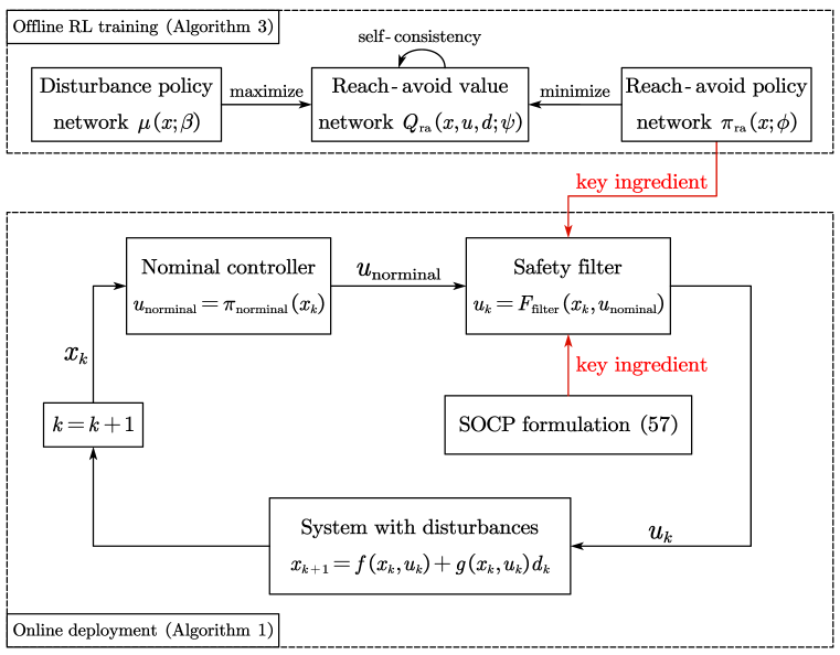
Figure 1: Illustration of the proposed methods, including offline RL training and online SOCP-based safety filtering.

Input: learned reach-avoid policy $\pi_{\rm ra}$, potentially unsafe nominal controller $\pi_{\rm nominal}$, terminal safe controller $\pi_{\rm terminal}$.

1

2Observe the current state $\overline{x}$ and get the nominal input $\overline{u}=\pi_{\rm nominal}(\overline{x})$.

3Generate the nominal trajectory $\mathcal{T}$ using $\pi_{\rm ra}$ with $z_{0}=\overline{x}$ and $v_{0}=\overline{u}$, which is detailed in (47).

4Solve the SOCP problem (57). Obtain $V_{\rm ra}^{*}$, $\mathbf{\Phi}_{u}^{*}$ and ${\mathbf{\Phi}_{x}^{*}}$. (We assume $V_{\rm ra}^{*}\leq 0$ for the first computation.)

5Update $\mathbf{K}$ with $\mathbf{K}=\mathbf{\Phi}_{u}^{*}{\mathbf{\Phi}_{x}^{*}}^{-1}$.

6Execute $u=v_{0}$ at current state.

7for $k=1,2,\cdots$ do

8      

9      Observe the current state $\overline{x}$ and get the nominal input $\overline{u}=\pi_{\rm nominal}(\overline{x})$.

10      Generate the nominal trajectory $\mathcal{T}$ using $\pi_{\rm ra}$ with $z_{0}=\overline{x}$ and $v_{0}=\overline{u}$, which is detailed in (47).

11      Solve the SOCP problem (57). Otain $V_{\rm ra}^{*}$, $\mathbf{\Phi}_{u}^{*}$ and ${\mathbf{\Phi}_{x}^{*}}$.

12      if $V_{\rm ra}^{*}\leq 0$ then

13             Reset $k=0$.

14            Update the nominal trajectory $\mathcal{T}$ with the results obtained in line 1.

15            Go to line 1 with system responses $\mathbf{\Phi}_{u}^{*}$ and ${\mathbf{\Phi}_{x}^{*}}$ obtained in line 1.

16       else

17            

18            Abandon the results of line 1 and 1.

19            if $k\leq T$ then

20                   Execute $u=v_{k}+\Sigma_{j=1}^{k}{\mathbf{K}^{k,j}\Delta x_{j}}$ at current state.

21             else

22                   Execute $u=\pi_{\rm terminal}(x_{k})$ at current state.

23             end if

24            

25       end if

26      

27 end for

Algorithm 1 Online deployment of the proposed safety filter

The execution procedure of the proposed safety filter is summarized in Algorithm 1. We assume that the first-time computation of the SOCP problem (from line 1 to 1) yields a $V_{\rm ra}^{*}\leq 0$, which is similar to the initial feasibility assumption for RMPC. We will show that the proposed safety filter guarantees persistent robust constraint satisfaction in Theorem 5.

We also provide a diagram that illustrates the overall design of the proposed methods in Fig. 1. The two key ingredients of our approach are the neural network reach-avoid policy trained offline and the SOCP formulation for online verification. Note that the SOCP formulation (57) provides the worst-case reach-avoid value $V_{\rm ra}^{*}$ and the optimal linear feedback stabilizing controller $\mathbf{K}$ simultaneously. The latter will be used for at most $T$ following timesteps, if the SOCP results at these steps all have positive $V_{\rm ra}^{*}$. Therefore the timestep index $k$ is actually entangled with the safety filter $F_{\rm filter}$, which is omitted in Fig. 1 for simplicity.

V RL for Robust Reach-Avoid Problems

In this section, we present an RL approach for solving the robust reach-avoid problems. Note that the Hamilton-Jacobi formulation (6) is for continuous-time systems with a finite horizon. Here we address discrete-time systems under infinite horizon.

We consider a general setting for discrete-time systems with disturbances,

$$x_{k+1}=F(x_{k},u_{k},d_{k}),\quad x\in\mathcal{S},u\in\mathcal{U},d\in\mathcal{D}.$$ (19)

The control input $u$ follows policy $\pi:\mathcal{S}\rightarrow\mathcal{U}$ and disturbance $d$ follows policy $\mu:\mathcal{S}\rightarrow\mathcal{D}$. The safety constraint is $h(x)\leq 0$. The target constraint is $l(x)\leq 0$. The avoiding set $\mathcal{A}$ is defined as $\mathcal{A}=\left\{x\mathrel{}\middle|\mathrel{}h(x)>0\right\}$. The target set $\mathcal{R}$ is defined as $\mathcal{R}=\left\{x\mathrel{}\middle|\mathrel{}l(x)\leq 0\right\}$.

The above settings cover the problem formulation in the previous section. (12) is a special case of (19). (13) implies that $h(x)=\max_{i}\left\{H_{x}^{i,:}x-h_{x}^{i}\right\}$ and (16) implies that $l(x)=\max_{i}\left\{R_{x}^{i,:}x-r_{x}^{i}\right\}$.

We define the following reach-avoid value function. Our approach is inspired by [38, 30].

Definition 1 (reach-avoid value functions).

1. Let $\mathcal{T}(x,\tau)$ denote a trajectory of the system (19) starting at $x$ with a finite horizon $\tau$, i.e., $\mathcal{T}(x,\tau)=\left\{x_{0}=x,u_{0},d_{0},x_{1},u_{1},d_{1},\cdots,x_{\tau},u_{\tau},d_{\tau}\right\}$. The reach-avoid value of a finite trajectory $\mathcal{T}(x,\tau)$ is defined as

   $$V_{\rm ra}(\mathcal{T}(x,\tau))=\max\left\{\max_{0\leq t\leq\tau,t\in\mathbb{N}}\left\{h(x_{t})\right\},l(x_{\tau})\right\}.$$ (20)

2. The reach-avoid value function of a protagonist policy $\pi$ and an adversary policy $\mu$ is defined as

   $$V_{\rm ra}^{\pi,\mu}(x)=\min_{\tau\in\mathbb{N}}\left\{V_{\rm ra}(\mathcal{T}(x,\tau))\right\},$$ (21)

   in which the trajectory $\mathcal{T}(x,\tau)$ is obtained by starting at $x_{0}=x$ and choosing $u_{t}=\pi(x_{t}),a_{t}=\mu(x_{t})$ for $0\leq t\leq\tau$.

3. The reach-avoid value function of a protagonist policy $\pi$ is defined as

   $$V_{\rm ra}^{\pi}(x)=\max_{\mu}\left\{V_{\rm ra}^{\pi,\mu}(x)\right\}.$$ (22)

4. The optimal reach-avoid value function is defined as

   $$V_{\rm ra}^{*}(x)=\min_{\pi}\left\{V_{\rm ra}^{\pi}(x)\right\}.$$ (23)

The reach-avoid value of a finite trajectory reflects whether the requirement of reaching $\mathcal{R}$ and avoiding $\mathcal{A}$ is fulfilled. For the reaching of $R$, the target constraint is imposed on the last timestep $\tau$. For the avoiding of $A$, the safety constraint is imposed on every timestep $0\leq t\leq\tau$. If $V_{\rm ra}(\mathcal{T}(x,\tau))\leq 0$, the requirement of reaching and avoiding are both achieved in this finite trajectory $\mathcal{T}(x,\tau)$. For a pair of policy $\pi$ and $\mu$, the reach-avoid value function chooses the optimal horizon $\tau$ such that the reach-avoid value of the corresponding trajectory $\mathcal{T}(x,\tau)$ is minimum, which is the best performance that can be achieved on the goal of reach-avoid. The reach-avoid value function of a policy $\pi$ reflects its capability of reach-avoid under worst-case disturbances. The optimal reach-avoid value function is associated with the best policy for the goal of reach-avoid under worst-case disturbances. We further define the reach-avoid sets as follows.

Definition 2 (reach-avoid sets).

1. The reach-avoid set for a policy $\pi$ is the zero-sublevel set of its reach-avoid value function, i.e.,

   $$S_{\rm ra}^{\pi}=\left\{x\mid V_{\rm ra}^{\pi}(x)\leq 0\right\}.$$ (24)

2. The maximal reach-avoid set is the zero-sublevel set of the optimal reach-avoid value function, i.e.,

   $$S_{\rm ra}^{*}=\left\{x\mid V_{\rm ra}^{*}(x)\leq 0\right\}.$$ (25)

For states outside the maximal reach-avoid set $S_{\rm ra}^{*}$, there is no policy that can drive the system to the target set while satisfying the safety constraints, under worst-case disturbances.

Since the reach-avoid value functions are defined on infinite horizon, they naturally hold a recursive structure with dynamic programming, which is referred to as the self-consistency condition, just like the common value functions in the standard RL setting. We have the following theorem.

Theorem 1 (self-consistency conditions for reach-avoid value functions).

Suppose $x^{\prime}$ is the successive state of $x$. The following self-consistency conditions hold for reach-avoid value functions, i.e.,

$$V_{\rm ra}^{\pi,\mu}(x)=\max\left\{h(x),\min\left\{l(x),V_{\rm ra}^{\pi,\mu}\left(x^{\prime}\right)\right\}\right\},$$ (26)

$$V_{\rm ra}^{\pi}(x)=\max\left\{h(x),\min\left\{l(x),\max_{d\in\mathcal{D}}V_{\rm ra}^{\pi}\left(x^{\prime}\right)\right\}\right\},$$ (27)

$$V_{\rm ra}^{*}(x)=\max\left\{h(x),\min\left\{l(x),\min_{u\in\mathcal{U}}\max_{d\in\mathcal{D}}V_{\rm ra}^{*}\left(x^{\prime}\right)\right\}\right\}.$$ (28)

Proof.

We first prove (26). Let $x^{\prime}$ denote the successive state of $x$ when the system is driven by $\pi$ and $\mu$, i.e., $x^{\prime}=F(x,\pi(x),\mu(x))$. We have

$$V_{\rm ra}^{\pi,\mu}(x)=\min_{\tau\geq 0}\left\{V_{\rm ra}(\mathcal{T}(x,\tau))\right\}$$ (29)

$$=\min\left\{V_{\rm ra}(\mathcal{T}(x,0)),\min_{\tau\geq 1}\left\{V_{\rm ra}(\mathcal{T}(x,\tau))\right\}\right\}$$

$$=\min\left\{V_{\rm ra}(\mathcal{T}(x,0)),\max\left\{h(x),\min_{\tau\geq 0}\left\{V_{\rm ra}(\mathcal{T}(x^{\prime},\tau))\right\}\right\}\right\}$$

$$=\min\left\{\max\left\{l(x),h(x)\right\},\max\left\{h(x),V_{\rm ra}^{\pi,\mu}(x^{\prime})\right\}\right\}$$

$$=\max\left\{h(x),\min\left\{l(x),V_{\rm ra}^{\pi,\mu}\left(x^{\prime}\right)\right\}\right\},$$

in which the second equality follows from manipulating the index of subscript $\tau$ based on the definition of $V_{\rm ra}(\mathcal{T}(x,\tau))$, and the last equality follows from the relationship $\min\{\max\{a,b\},\max\{b,c\}\}=\max\{b,\min\{a,c\}\}$.

(27) and (28) can be obtained by further considering Bellman’s principle of optimality. ∎

The self-consistency conditions for reach-avoid value functions in Theorem 1 are not contraction mappings, which is different from the standard RL setting. Therefore, they can not be directly utilized for policy iteration. Following the method in [38], we introduce a discount factor $\gamma_{\rm ra}$ into the formulations and obtain three contractive self-consistency operators.

Definition 3 (reach-avoid self-consistency operators).

Suppose $0<\gamma_{\rm ra}<1$. The reach-avoid self-consistency operators are defined as

$$\left[T_{\rm ra}^{\pi,\mu}(V_{\rm ra})\right](x)=(1-\gamma_{\rm ra})\max\left\{l(x),h(x)\right\}$$ (30)

$$+\gamma_{\rm ra}\max\left\{h(x),\min\left\{l(x),V_{\rm ra}\left(x^{\prime}\right)\right\}\right\},$$

$$\left[T_{\rm ra}^{\pi}(V_{\rm ra})\right](x)=(1-\gamma_{\rm ra})\max\left\{l(x),h(x)\right\}$$ (31)

$$+\gamma_{\rm ra}\max\left\{h(x),\min\left\{l(x),\max_{d\in\mathcal{D}}V_{\rm ra}\left(x^{\prime}\right)\right\}\right\},$$

$$\left[T_{\rm ra}(V_{\rm ra})\right](x)=(1-\gamma_{\rm ra})\max\left\{l(x),h(x)\right\}$$ (32)

$$+\gamma_{\rm ra}\max\left\{h(x),\min\left\{l(x),\min_{u\in\mathcal{U}}\max_{d\in\mathcal{D}}V_{\rm ra}\left(x^{\prime}\right)\right\}\right\}.$$

Theorem 2 (monotone contraction).

Let $T$ denote any of ${T_{\rm ra}^{\pi,\mu},T_{\rm ra}^{\pi},T_{\rm ra}}$.

1. Given any $V_{\rm ra},\widetilde{V}_{\rm ra}$, we have

   $$\left\|T(V_{\rm ra})-T(\widetilde{V}_{\rm ra})\right\|_{\infty}\leq\gamma_{\rm ra}\left\|V_{\rm ra}-\widetilde{V}_{\rm ra}\right\|_{\infty}.$$ (33)

2. Suppose $V_{\rm ra}(x)\geq\widetilde{V}_{\rm ra}(x)$ holds for any $x\in\mathcal{S}$. Then we have

   $$[T(V_{\rm ra})](x)\geq[T(\widetilde{V}_{\rm ra})](x),\quad\forall x\in\mathcal{S}.$$ (34)

Proof.

We only prove the monotone contraction for $T_{\rm ra}$, while the proof for $T_{\rm ra}^{\pi}$ and $T_{\rm ra}^{\pi,\mu}$ is similar. We have

$$[T_{\rm ra}(V_{\rm ra})](x)-[T_{\rm ra}(\widetilde{V}_{\rm ra})](x)$$ (35)

$$= \gamma_{\rm ra}\max\left\{h(x),\min\left\{l(x),\min_{u\in\mathcal{U}}\max_{d\in\mathcal{D}}V_{\rm ra}\left(x^{\prime}\right)\right\}\right\}$$

$$-\gamma_{\rm ra}\max\left\{h(x),\min\left\{l(x),\min_{u\in\mathcal{U}}\max_{d\in\mathcal{D}}\widetilde{V}_{\rm ra}\left(x^{\prime}\right)\right\}\right\}.$$

We have

$$\left\|T_{\rm ra}(V_{\rm ra})-T_{\rm ra}(\widetilde{V}_{\rm ra})\right\|_{\infty}$$ (36)

$$\leq \gamma_{\rm ra}\max\limits_{u\in\mathcal{U}}\max\limits_{d\in\mathcal{D}}\left|V_{\rm ra}(f(x,u,a))-\widetilde{V}_{\rm ra}(f(x,u,a))\right|$$

$$\leq \gamma_{\rm ra}\left\|V_{\rm ra}-\widetilde{V}_{\rm ra}\right\|_{\infty}.$$

The first inequality in (36) follows from the relationship

$$\left|\min_{x}\max_{y}f(x,y)-\min_{x}\max_{y}g(x,y)\right|$$ (37)

$$\leq\max_{x}\max_{y}\left|f(x,y)-g(x,y)\right|.$$

Since $\max$ and $\min$ operations are monotone, the monotonicity of $T_{\rm ra}$ is obvious. ∎

In the following proposition, we show that if $\gamma_{\rm ra}$ is sufficiently close to 1, the fixed points of the self-consistency operators approach the original reach-avoid value functions.

Proposition 1.

Let $T$ denote any of ${T_{\rm ra}^{\pi,\mu},T_{\rm ra}^{\pi},T_{\rm ra}}$, and $V_{\rm ra}^{d}$ denote the fixed point of operator $T$, i.e., $T(V_{\rm ra}^{d})=V_{\rm ra}^{d}$. Let $V_{\rm ra}$ denote the corresponding original reach-avoid value function in Definition 1. Then we have $\lim_{\gamma_{\rm ra}\rightarrow 1}V_{\rm ra}^{d}(x)=V_{\rm ra}(x)$.

Proof.

The key is to define a discounted version of reach-avoid values. The original definition of $V_{\rm ra}^{\pi,\mu}(x)$ is given by $V_{\rm ra}^{\pi,\mu}(x)=\min_{\tau\in\mathbb{N}}\left\{V_{\rm ra}(\mathcal{T}(x,\tau))\right\}$. Let $\left\{x_{t}\right\}$ denote the trajectory of the system when it is driven by $\pi$ and $\mu$, starting from $x_{0}=x$. We define the discounted reach-avoid value as

$$D(x) =(1-\gamma_{\rm ra})\max\left\{l(x_{0}),h(x_{0})\right\}+\gamma_{\rm ra}\max\left\{h(x_{0}),\right.$$ (38)

$$\min\left\{l(x_{0}),\right.\left.(1-\gamma_{\rm ra})\max\left\{l(x_{1}),h(x_{1})\right\}\right.$$

$$\left.+\gamma_{\rm ra}\max\left\{h(x_{1}),\min\left\{l(x_{1}),\cdots\right\}\right\}\right\},$$

It can be verified that $D$ is the explicit form of the fixed point of $T_{\rm ra}^{\pi,\mu}$, i.e., $D=T_{\rm ra}^{\pi,\mu}(D)$. Forcing $\gamma_{\rm ra}$ to be sufficiently close to 1, we have $\lim_{\gamma_{\rm ra}\rightarrow 1}D(x)=V_{\rm ra}^{\pi,\mu}(x)$. The proof is similar for $T_{\rm ra}^{\pi}$ and $T_{\rm ra}$. ∎

Since the reach-avoid self-consistency operators are monotone contractions, we can utilize policy iteration to solve for the reach-avoid sets. The policy iteration algorithm is shown in Algorithm 2, in which we iterate between policy evaluation and policy improvement. The former evaluates the reach-avoid value function of the current policy $\pi$, by finding the worst-case disturbances for $\pi$. The latter finds a better policy on the performance of reach-avoid, by solving a maximin problem. The convergence of the proposed policy iteration is shown in Theorem 3.

Input: initial policy $\pi_{0}$.

1 for each iteration $k$ do

2       (policy evaluation)

3      Solve for $V_{\rm ra}^{\pi_{k}}$ such that $V_{\rm ra}^{\pi_{k}}=T_{\rm ra}^{\pi_{k}}(V_{\rm ra}^{\pi_{k}})$.

4      (policy improvement)

5      $\pi_{k+1}=\underset{\pi}{\mathrm{arg}\min}\left\{T_{\rm ra}^{\pi}\left(V_{\rm ra}^{\pi_{k}}\right)\right\}$.

6 end for

Algorithm 2 Policy iteration for robust reach-avoid problems

Theorem 3 (monotone convergence of policy iteration).

The sequence $\left\{V_{\rm ra}^{\pi_{k}}\right\}$ generated by Algorithm 2 converges monotonically to the fixed point $V_{\rm ra}^{*}$ of $T_{\rm ra}$, i.e., $T_{\rm ra}(V_{\rm ra}^{*})=V_{\rm ra}^{*}$.

Proof.

The key is to exploit the monotonicity and contraction of $T_{\rm ra}^{\pi}$ and $T_{\rm ra}$. First we establish the following recursive relationship:

$$V_{\rm ra}^{\pi_{k}}\geq T_{\rm ra}(V_{\rm ra}^{\pi_{k}})\geq V_{\rm ra}^{\pi_{k+1}}\geq V_{\rm ra}^{*}.$$ (39)

With the definition of $T_{\rm ra}$ and policy improvement, we have

$$T_{\rm ra}(V_{\rm ra}^{\pi_{k}})=T_{\rm ra}^{\pi_{k+1}}(V_{\rm ra}^{\pi_{k}})\leq T_{\rm ra}^{\pi_{k}}(V_{\rm ra}^{\pi_{k}})=V_{\rm ra}^{\pi_{k}}.$$ (40)

Utilizing the monotonicity and contraction of $T_{\rm ra}^{\pi_{k+1}}$, together with $V_{\rm ra}^{\pi_{k}}\geq T_{\rm ra}^{\pi_{k+1}}(V_{\rm ra}^{\pi_{k}})$, we have

$$V_{\rm ra}^{\pi_{k}} \geq T_{\rm ra}(V_{\rm ra}^{\pi_{k}})=T_{\rm ra}^{\pi_{k+1}}(V_{\rm ra}^{\pi_{k}})$$ (41)

$$\geq(T_{\rm ra}^{\pi_{k+1}})^{\infty}(V_{\rm ra}^{\pi_{k}})=V_{\rm ra}^{\pi_{k+1}}.$$

Utilizing the monotonicity and contraction of $T_{\rm ra}$, and $T_{\rm ra}(V_{\rm ra}^{\pi_{k+1}})\leq T_{\rm ra}^{\pi_{k+1}}(V_{\rm ra}^{\pi_{k+1}})=V_{\rm ra}^{\pi_{k+1}}$, we have

$$V_{\rm ra}^{*}=(T_{\rm ra})^{\infty}(V_{\rm ra}^{\pi_{k+1}})\leq\cdots\leq V_{\rm ra}^{\pi_{k+1}}.$$ (42)

So the recursive relationship (39) holds. The sequence $\left\{V_{\rm ra}^{\pi_{k}}\right\}$ generated by policy iteration is monotonically decreasing and bounded by $V_{\rm ra}^{\pi_{0}}\geq V_{\rm ra}^{\pi_{k}}\geq V_{\rm ra}^{*}$, so it converges. The convergence implies that $V_{\rm ra}^{\pi_{k}}=T_{\rm ra}(V_{\rm ra}^{\pi_{k}})=V_{\rm ra}^{\pi_{k+1}}$, which means that the convergence point is the fixed point of $T_{\rm ra}$. ∎

The policy iteration approach enjoys rigorous convergence guarantee and the policy is guaranteed to fulfill the goal of reach-avoid for states inside its reach-avoid set. However, it requires state-wise computation and is computationally prohibitive for continuous state spaces. Still, it paves the way for the design of an actor-critic deep RL algorithm, which is of high scalability and applicable to complex systems with continuous state and action spaces.

We utilize the action reach-avoid values for the actor-critic algorithm. The relationship between the action reach-avoid values and the reach-avoid values is similar to that of common action values and common values in the standard RL setting. The algorithm includes three neural networks: the reach-avoid policy network $\pi_{\rm ra}(x;\phi)$, the disturbance network $\mu(x;\beta)$ and the reach-avoid value network $Q_{\rm ra}(x,u,d;\psi)$. $\phi$, $\beta$ and $\psi$ denote the network parameters. For a set $\mathcal{D}$ of collected samples, the loss function for $Q_{\rm ra}(x,u,a;\psi)$ is

$$L_{Q_{\rm ra}}(\psi)=\mathbb{E}_{(x,u,d,h,l,x^{\prime})\sim\mathcal{D}}\left\{\left(Q_{\rm ra}(x,u,d;\psi)-\hat{Q}_{\rm ra}\right)^{2}\right\},$$ (43)

where

$$\hat{Q}_{\rm ra}=(1-\gamma_{\rm ra})\max\left\{l(x),h(x)\right\}$$ (44)

$$+\gamma_{\rm ra}\max\left\{h(x),\min\left\{l(x),Q_{\rm ra}\left(x^{\prime},u^{\prime},d^{\prime};\bar{\psi}\right)\right\}\right\},$$

in which $u^{\prime}=\pi_{\rm ra}(x^{\prime};\phi)$ and $d^{\prime}=\mu(x^{\prime};\beta)$. $\bar{\psi}$ denotes target network parameters for $Q_{\rm ra}$, which follows the standard design in RL algorithms. This loss function is based on the reach-avoid self-consistency operators. $\pi_{\rm ra}(x;\phi)$ aims to minimize the reach-avoid value. Its loss function is

$$L_{\pi_{\rm ra}}(\phi)=\mathbb{E}_{x\sim\mathcal{D}}\left\{Q_{\rm ra}\left(x,\pi_{\rm ra}(x;\phi),\mu(x;\beta);\psi\right)\right\}.$$ (45)

$\mu(x;\beta)$ aims to maximize the reach-avoid value. Its loss function is

$$L_{\mu}(\beta)=-\mathbb{E}_{x\sim\mathcal{D}}\left\{Q_{\rm ra}\left(x,\pi_{\rm ra}(x;\phi),\mu(x;\beta);\psi\right)\right\}.$$ (46)

The overall algorithm is summarized in Algorithm 3.

Input: network parameters $\psi$, $\phi$ and $\beta$, target network parameter $\bar{\psi}\leftarrow\psi$, learning rate $\eta$, target smoothing coefficient $\tau$, replay buffer $\mathcal{D}\leftarrow\varnothing$.

1 for each iteration do

2       for each system step do

3             Sample control input $u_{t}\sim\pi_{\rm ra}(x_{t};\phi)$;

4            Sample disturbance $d_{t}\sim\mu(x_{t};\beta)$;

5            Observe next state $x_{t+1}$, safety constraint value $h_{t}$, target constraint value $l_{t}$;

6            Store transition $\mathcal{D}\leftarrow\mathcal{D}\cup\left\{\left(x_{t},u_{t},d_{t},h_{t},l_{t},x_{t+1}\right)\right\}$.

7       end for

8      

9      for each gradient step do

10             Sample a batch of data from $\mathcal{D}$;

11            Update reach-avoid value function $\psi\leftarrow\psi-\eta\nabla_{\psi}L_{Q_{\rm ra}}(\psi)$;

12            Update protagonist policy $\phi\leftarrow\phi-\eta\nabla_{\phi}L_{\pi_{\rm ra}}(\phi)$;

13            Update adversary policy $\beta\leftarrow\beta-\eta\nabla_{\beta}L_{\mu}(\beta)$;

14            Update target network $\bar{\psi}\leftarrow\tau\psi+(1-\tau)\psi$.

15       end for

16      

17 end for

Algorithm 3 Actor-critic algorithm for robust reach-avoid problems

VI Online Safety Verificaiton

As discussed in previous sections, the RL method for robust reach-avoid problems enjoys considerable scalability and is applicable to complex systems. However, the safety assurance is lost. In this section, we discuss how to reestablish the guarantee of robust constraint satisfaction.

Given an initial state, we can generate a nominal trajectory using the learned reach-avoid policy $\pi_{\rm ra}$. It is not enough to just check that the reach-avoid value of this nominal trajectory is negative. We need to further verify that the reach-avoid Values of all possible trajectories that deviate from the nominal one due to disturbances are negative. There are two options to accomplish this goal. The first is to directly check that the constraints are satisfied for all possible realizations of the disturbance sequence, which is similar to the idea of robust open-loop MPC. The second is to permit an additional feedback controller that actively stabilizes the system back to the nominal trajectory and then check the robust constraint satisfaction, which is similar to the idea of tube-based MPC [43]. We adopt the second approach, since in the first approach the set of all possible trajectories can grow very large, resulting in misleadingly small safe sets for safety filters.

In tube-based MPC approaches, the stabilizing feedback controllers are typically designed offline and the nominal trajectories are optimized online [43]. Recent advances utilize system level synthesis to jointly optimize the nominal trajectory and the feedback controller on-the-fly, with the benefit of significantly reducing conservatism [40, 44, 45]. However, nonlinear RMPC methods using system level synthesis involve solving non-convex optimization problems, which is computationally prohibitive [44, 45]. Inspired by these works, in this paper, we utilize system level synthesis to only optimize the feedback controller for the smallest worst-case reach-avoid value, and establish a SOCP formulation that can be solved efficiently.

VI-A Establishing Error Dynamics

Let $T$ denote the prediction horizon. For a given state $\overline{x}$ and an output $\overline{u}$ from the nominal controller, the nominal trajectory $\mathcal{T}(z_{0},T)=\left\{z_{0},v_{0},z_{1},\cdots,z_{T},v_{T}\right\}$ is generated as

$$z_{k+1}=f(z_{k},v_{k}),\quad v_{k+1}=\pi_{\rm ra}(z_{k+1}),\quad k=0,\cdots,T-1,$$ (47)

$$\text{s.t.}\quad z_{0}=\overline{x},\quad v_{0}=\overline{u}.$$

in which $\pi_{\rm ra}$ denotes the reach-avoid policy learned with Algorithm 3.

To design a feedback controller that stabilizes the system back to the nominal trajectory, firstly we need to establish the error dynamics. For a nonlinear system, it is common to linearize the system around the nominal trajectory and bound the linearization error [18, 35, 44]. We adopt the method proposed in [44].

For $0\leq k\leq T$, we have

$$f\left(x_{k},u_{k}\right)= f\left(z_{k},v_{k}\right)+A_{k}^{f}\left(x_{k}-z_{k}\right)+B_{k}^{f}\left(u_{k}-v_{k}\right)$$ (48)

$$+r_{f}\left(x_{k}-z_{k},u_{k}-v_{k}\right),$$

in which $A_{k}^{f}\in\mathbb{R}^{n_{x}\times n_{x}}$ and $B_{k}^{f}\in\mathbb{R}^{n_{x}\times n_{u}}$ is given by

$$A_{k}^{f}=\left.\frac{\partial f}{\partial x}\right|_{x=z_{k},u=v_{k}},\quad B_{k}^{f}=\left.\frac{\partial f}{\partial u}\right|_{x=z_{k},u=v_{k}}.$$ (49)

and $r_{f}\left(x_{k}-z_{k},u_{k}-v_{k}\right)$ is the Lagrange remainder. We also have

$$g\left(x_{k},u_{k}\right)d_{k}= g\left(z_{k},v_{k}\right)d_{k}+\left(I_{n_{x}}\otimes d_{k}^{\top}\right)A_{k}^{g}\left(x_{k}-z_{k}\right)$$ (50)

$$+\left(I_{n_{x}}\otimes d_{k}^{\top}\right)B_{k}^{g}\left(u_{k}-v_{k}\right)$$

$$+r_{g}\left(x_{k}-z_{k},u_{k}-v_{k},d_{k}\right),$$

in which $A_{k}^{g}\in\mathbb{R}^{n_{x}n_{d}\times n_{x}}$ and $B_{k}^{g}\in\mathbb{R}^{n_{x}n_{d}\times n_{u}}$ is defined as

$$A_{k}^{g}=\left(A_{k}^{g_{1,:}},A_{k}^{g_{2,:}},\cdots,A_{k}^{g_{n_{x},:}}\right)^{\top},$$ (51)

$$B_{k}^{g}=\left(B_{k}^{g_{1,:}},B_{k}^{g_{2,:}},\cdots,B_{k}^{g_{n_{x},:}}\right)^{\top},$$ (52)

with $A_{k}^{g_{i,:}}\in\mathbb{R}^{n_{x}\times n_{d}}$ and $B_{k}^{g_{i,:}}\in\mathbb{R}^{n_{u}\times n_{d}}$ given by

$$A_{k}^{g_{i,:}}=\left.\frac{\partial g_{i,:}}{\partial x}\right|_{x=z_{k},u=v_{k}},\quad B_{k}^{g_{i,:}}=\left.\frac{\partial g_{i,:}}{\partial u}\right|_{x=z_{k},u=v_{k}}.$$ (53)

The error term $r_{g}\left(x_{k}-z_{k},u_{k}-v_{k},d_{k}\right)$ is determined by $d_{k}$ and the Lagrange remainder of $g\left(x_{k},u_{k}\right)$.

The overall linearization error $r=r_{f}\left(x_{k}-z_{k},u_{k}-v_{k}\right)+r_{g}\left(x_{k}-z_{k},u_{k}-v_{k},d_{k}\right)$ can be overbound by

$$\left|r_{i}\right|\leq\|e_{k}\|_{\infty}^{2}\mu_{i},\quad i=1,2,\cdots,n_{x},$$ (54)

$$\forall x_{k},z_{k}\in\mathcal{X},\quad\forall u_{k},v_{k}\in\mathcal{U},\quad\forall d_{k}\in\mathcal{D},$$

in which $e_{k}=\left[(x_{k}-z_{k})^{\top},(u_{k}-v_{k})^{\top}\right]^{\top}\in\mathbb{R}^{n_{x}+n_{u}}$ and $\mu_{i}$ denote the worst-case curvature. See [44] for more details.

Define $\Delta x_{k}=x_{k}-z_{k}$ and $\Delta u_{k}=u_{k}-v_{k}$. The error dynamics is given by

$$\Delta x_{k+1}=A_{k}^{f}\Delta x_{k}+B_{k}^{f}\Delta u_{k}+w_{k},\quad k=0,\cdots,T-1,$$ (55)

$$\begin{aligned} \text{s.t.}\quad\Delta x_{0}=0,\quad\Delta u_{0}=0,\end{aligned}$$

in which $w_{k}$ is given by

$$w_{k}= r_{k}+g\left(z_{k},v_{k}\right)d_{k}+\left(I_{n_{x}}\otimes d_{k}^{\top}\right)A_{k}^{g}\Delta x_{k}$$ (56)

$$+\left(I_{n_{x}}\otimes d_{k}^{\top}\right)B_{k}^{g}\Delta u_{k}.$$

VI-B SOCP Approach for Worst-case Reach-Avoid Values

Following the notations in (8), we denote the stacked states, nominal states, inputs, nominal inputs and disturbances as $\mathbf{x}=[x_{1}^{\top},\cdots,x_{T}^{\top}]^{\top}$, $\mathbf{z}=[z_{1}^{\top},\cdots,z_{T}^{\top}]^{\top}$, $\mathbf{u}=[u_{1}^{\top},\cdots,u_{T}^{\top}]^{\top}$, $\mathbf{v}=[v_{1}^{\top},\cdots,v_{T}^{\top}]^{\top}$, $\mathbf{d}=[d_{0}^{\top},\cdots,d_{T-1}^{\top}]^{\top}$, respectively. We have $\mathbf{\Delta x}=\mathbf{x}-\mathbf{z}$ and $\mathbf{\Delta u}=\mathbf{u}-\mathbf{v}$. Also let $\mathcal{V}_{\mathcal{D}}$ denote the set of vertices for the polytope $\mathcal{D}$.

Given the error dynamics (55), we can design a feedback controller to stabilize the system back to the nominal trajectory. The controller follows the causal linear state-feedback design, i.e., $\mathbf{\Delta u}=\mathbf{K}\mathbf{\Delta x}$, in which $\mathbf{K}\in\mathcal{L}^{T,n_{u}\times n_{x}}$. The goal is to minimize the worst-case reach-avoid value $V_{\rm ra}^{*}$ for any closed-loop trajectories of the system (12). If $V_{\rm ra}^{*}\leq 0$, the system is guaranteed to be safely guided back to the target set. Leveraging the tools of system level synthesis, we establish a SOCP formulation to accomplish this goal, which is summarized in (57). $n_{H_{x}}$ denotes the number of rows in $H_{x}$ and the same goes for $n_{H_{u}}$ and $n_{R_{x}}$. The only nonlinear part of (57) is (57k), which belongs to second-order cone constraints. This is not possible for RMPC approaches even in the linear system case [40], since the nominal trajectory and system responses are both decision variables and are coupled in (57b).

$$\min_{\mathbf{\Phi}_{x},\mathbf{\Phi}_{u},\mathbf{\Sigma},\lambda,\eta,V_{\mathrm{ra}}} V_{\mathrm{ra}}$$ (57a)

$$\mathrm{s}.\mathrm{t}.\qquad\, \left[\begin{matrix}I-\mathcal{Z}\mathbf{A}&-\mathcal{Z}\mathbf{B}\\ \end{matrix}\right]\begin{bmatrix}\mathbf{\Phi}_{x}\\ \mathbf{\Phi}_{u}\end{bmatrix}=\mathbf{\Sigma},$$ (57b)

$$\left|I_{n_{x}}^{i,:}g\left(z_{0},v_{0}\right)d\right|\leq\sigma_{0,i},\quad\forall i=1,\cdots,n_{x},\quad\forall d\in\mathcal{V}_{\mathcal{D}},$$ (57c)

$$\begin{aligned} \lambda_{k}\mu_{i}&+\left|I_{n_{x}}^{i,:}g\left(z_{k},v_{k}\right)d\right|+\left\|I_{n_{x}}^{i,:}\left(I_{n_{x}}\otimes d^{\top}\right)A_{k}^{g}\mathbf{\Phi}_{x}^{k,1:k}\right\|_{1}+\left\|I_{n_{x}}^{i,:}\left(I_{n_{x}}\otimes d^{\top}\right)B_{k}^{g}\mathbf{\Phi}_{u}^{k,1:k}\right\|_{1}\leq\sigma_{k,i},\\ &\forall k=1,\cdots,T-1,\quad\forall i=1,\cdots,n_{x},\quad\forall d\in\mathcal{V}_{\mathcal{D}},\\ \end{aligned}$$ (57d)

$$\left\|\begin{pmatrix}\mathbf{\Phi}_{x}^{k,1:k}\\ \mathbf{\Phi}_{u}^{k,1:k}\end{pmatrix}\right\|_{\infty}\leq\eta_{k},\quad\forall k=1,\cdots,T-1,$$ (57e)

$$H_{x}^{i,:}z_{0}-h_{x}^{i}\leq V_{\mathrm{ra}},\quad\forall i=1,\cdots,n_{H_{x}},$$ (57f)

$$H_{x}^{i,:}z_{k}+\left\|H_{x}^{i,:}\mathbf{\Phi}_{x}^{k,1:k}\right\|_{1}-h_{x}^{i}\leq V_{\mathrm{ra}},\quad\forall k=1,\cdots,T,\quad\forall i=1,\cdots,n_{H_{x}},$$ (57g)

$$H_{u}^{i,:}v_{0}-h_{u}^{i}\leq V_{\mathrm{ra}},\quad\forall i=1,\cdots,n_{H_{u}},$$ (57h)

$$H_{u}^{i,:}v_{k}+\left\|H_{u}^{i,:}\mathbf{\Phi}_{u}^{k,1:k}\right\|_{1}-h_{u}^{i}\leq 0,\quad\forall k=1,\cdots,T,\quad\forall i=1,\cdots,n_{H_{u}},$$ (57i)

$$R_{x}^{i,:}z_{T}+\left\|R_{x}^{i,:}\mathbf{\Phi}_{x}^{T,:}\right\|_{1}-r_{x}^{i}\leq V_{\mathrm{ra}},\quad\forall i=1,\cdots,n_{R_{x}},$$ (57j)

$$\left\|\left(\frac{\lambda_{k}-1}{2},\eta_{k}\right)^{\top}\right\|_{2}\leq\frac{\lambda_{k}+1}{2},\quad\forall k=1,\cdots,T-1.$$ (57k)

 

The key of (57) is to overbound $w_{k}$ in (55) with $\Sigma_{k}\widetilde{w}_{k}$, in which the disturbance filter $\Sigma_{k}={\rm diag}(\sigma_{k,1},\cdots,\sigma_{k,n_{x}})$ and $\widetilde{w}_{k}\in\mathcal{B}_{\infty}^{n_{x}}$. Then utilize Lemma 1 to impose state and input constraints on the system responses $\mathbf{\Phi}_{x}$ and $\mathbf{\Phi}_{u}$. We formally prove the correctness of this SOCP formulation in the following theorem.

Theorem 4 (worst-case reach-avoid value).

Let $\mathbf{\Phi}_{x}^{*}$, $\mathbf{\Phi}_{u}^{*}$ and $V^{*}_{\rm ra}$ denote the optimal solution of (57). The overall feedback controller is constructed as $\mathbf{u}=\mathbf{v}+\mathbf{K}(\mathbf{x}-\mathbf{z})$, in which $\mathbf{K}=\mathbf{\Phi}_{u}^{*}{\mathbf{\Phi}_{x}^{*}}^{-1}$. Any close-loop trajecotry $\mathcal{T}(x_{0},T)$ of the system (12) under this feedback controller with $\mathbf{d}\in\mathcal{D}^{T}$ satisfies that $V_{\rm ra}(\mathcal{T}(x_{0},T))\leq V^{*}_{\rm ra}$.

Proof.

We first prove that $w_{k}$ in (55) is overbounded by $\Sigma_{k}\widetilde{w}_{k}$, in which the disturbance filter $\Sigma_{k}={\rm diag}(\sigma_{k,1},\cdots,\sigma_{k,n_{x}})$ and $\widetilde{w}_{k}\in\mathcal{B}_{\infty}^{n_{x}}$. With this overbound, we can conclude all possible behaviors of the error dynamics (55) are included in those of the new error dynamics as $\Delta x_{k+1}=A_{k}^{f}\Delta x_{k}+B_{k}^{f}\Delta u_{k}+\Sigma_{k}\widetilde{w}_{k}$. Then we can utilize Lemma 1 to obtain that $\mathbf{\Delta x}=\mathbf{\Phi}_{x}\mathbf{\widetilde{w}}$ and $\mathbf{\Delta u}=\mathbf{\Phi}_{u}\mathbf{\widetilde{w}}$ for $\mathbf{\widetilde{w}}\in\mathcal{B}_{\infty}^{Tn_{x}}$. It is suffice is to show that $|I_{n_{x}}^{i,:}w_{k}|\leq\sigma_{k,i}$. For $k=0$, it is obvious in (57c). For $1\leq k\leq T-1$, we have

$$|I_{n_{x}}^{i,:}w_{k}|\leq |I_{n_{x}}^{i,:}r_{k}|+|I_{n_{x}}^{i,:}g\left(z_{k},v_{k}\right)d_{k}|$$ (58)

$$+|I_{n_{x}}^{i,:}\left(I_{n_{x}}\otimes d_{k}^{\top}\right)A_{k}^{g}\Delta x_{k}|$$

$$+|I_{n_{x}}^{i,:}\left(I_{n_{x}}\otimes d_{k}^{\top}\right)B_{k}^{g}\Delta u_{k}|.$$

Utilizing (54), we have $|I_{n_{x}}^{i,:}r_{k}|\leq\left\|(\Delta x_{k},\Delta u_{k})^{\top}\right\|_{\infty}\mu_{i}$. With Lemma 1, we have $\Delta x_{k}=\mathbf{\Phi}_{x}^{k,1:k}\mathbf{\widetilde{w}}^{1:kn_{x}}$ and $\Delta u_{k}=\mathbf{\Phi}_{u}^{k,1:k}\mathbf{\widetilde{w}}^{1:kn_{x}}$. Since $\left\|\mathbf{\widetilde{w}}^{1:kn_{x}}\right\|_{\infty}=1$, together with (57e) and (57k), we have $|I_{n_{x}}^{i,:}r_{k}|\leq\lambda_{k}\mu_{i}$. With the definition of matrix one-norm, we have $|I_{n_{x}}^{i,:}\left(I_{n_{x}}\otimes d_{k}^{\top}\right)A_{k}^{g}\Delta x_{k}|\leq\left\|I_{n_{x}}^{i,:}\left(I_{n_{x}}\otimes d^{\top}\right)A_{k}^{g}\mathbf{\Phi}_{x}^{k,1:k}\right\|_{1}$ and $|I_{n_{x}}^{i,:}\left(I_{n_{x}}\otimes d_{k}^{\top}\right)B_{k}^{g}\Delta x_{k}|\leq\left\|I_{n_{x}}^{i,:}\left(I_{n_{x}}\otimes d^{\top}\right)B_{k}^{g}\mathbf{\Phi}_{u}^{k,1:k}\right\|_{1}$. Putting the above analysis together, we have

$$|I_{n_{x}}^{i,:}w_{k}|\leq |I_{n_{x}}^{i,:}r_{k}|+|I_{n_{x}}^{i,:}g\left(z_{k},v_{k}\right)d_{k}|$$ (59)

$$+\left\|I_{n_{x}}^{i,:}\left(I_{n_{x}}\otimes d_{k}^{\top}\right)A_{k}^{g}\mathbf{\Phi}_{x}^{k,1:k}\right\|_{1}$$

$$+\left\|I_{n_{x}}^{i,:}\left(I_{n_{x}}\otimes d_{k}^{\top}\right)B_{k}^{g}\mathbf{\Phi}_{u}^{k,1:k}\right\|_{1},$$

which aligns with (57d). Since the right-hand side of (59) is linear with $d$ and $\mathcal{D}$ is convex, we only need (57d) to hold for all $d\in\mathcal{V}_{\mathcal{D}}$.

Next we show that the worst-case reach-avoid value is bounded by $V_{\rm ra}$. For state constraints, we have

$$H_{x}^{i,:}x_{k}-h_{x}^{i} =H_{x}^{i,:}(z_{k}+\Delta x_{k})-h_{x}^{i}$$ (60)

$$=H_{x}^{i,:}z_{k}+H_{x}^{i,:}\Delta x_{k}-h_{x}^{i}$$

$$\leq H_{x}^{i,:}z_{k}+\left\|H_{x}^{i,:}\mathbf{\Phi}_{x}^{k,1:k}\right\|_{1}-h_{x}^{i},$$

in which the last inequality follows from the definition of vector one-norm and $\Delta x_{k}=\mathbf{\Phi}_{x}^{k,1:k}\mathbf{\widetilde{w}}^{1:kn_{x}}$. Similarly, the bounds for input constraints and target constraints can also be proved. Also, with Lemma (1), the overall feedback controller is given by $\mathbf{u}=\mathbf{v}+\mathbf{K}^{*}(\mathbf{x}-\mathbf{z})$. ∎

The execution procedure of the proposed safety filter is summarized in Algorithm 1. We show in the following theorem that this algorithm achieves persistent safety guarantee.

Theorem 5 (persistent safety guarantee).

Assume that the first-time computation of (57) yields a $V_{\rm ra}^{*}\leq 0$. Then the infinite-horizon closed-loop trajectory of the system (12) under the safety filter described with Algorithm 1 is guaranteed to satisfy the state constraints, i.e., $x_{k}\in\mathcal{X}$, $\forall k\geq 0$ and $\forall d_{k}\in\mathcal{D}$.

Proof.

Given a $V_{\rm ra}^{*}\leq 0$ and the corresponding $\mathbf{\Phi}_{x}^{*}$ and $\mathbf{\Phi}_{u}^{*}$, a closed-loop feedback controller is constructed as $\mathbf{u}=\mathbf{v}+\mathbf{K}(\mathbf{x}-\mathbf{z})$, in which $\mathbf{K}=\mathbf{\Phi}_{u}^{*}{\mathbf{\Phi}_{x}^{*}}^{-1}$. Based on Theorem 4, the closed-loop trajectory under this feedback controller satisfies that $x_{k}\in\mathcal{X}$, $0\leq k\leq T$ and $x_{T}\in\mathcal{R}$. As shown in Algorithm 1, at every following state, the SOCP problem (57) is solved. There may be two cases. If a $V_{\rm ra}^{*}>0$ is obtained, we choose the initially constructed feedback controller $\mathbf{u}=\mathbf{v}+\mathbf{K}(\mathbf{x}-\mathbf{z})$ for $1\leq k\leq T$ and the terminal controller $\pi_{\rm terminal}$ for $k\geq T+1$. Therefore, the state trajectory satisfies $x_{k}\in\mathcal{X}$. If a $V_{\rm ra}^{*}\leq 0$ is obtained, we reset $k=0$ and reconstruct the closed-loop feedback controller, which gets the situation back to the beginning. In either case, the safety of the system is guaranteed. ∎

VII Numerical Example

In this section, we demonstrate the effectiveness of our method through a numerical example. Consider the dynamics of a pendulum:

$$\begin{bmatrix}\dot{x}_{2}\\ \dot{x}_{2}\end{bmatrix}=\begin{bmatrix}x_{1}\\ \frac{3g}{2l}\sin\left(x_{1}\right)\end{bmatrix}+\begin{bmatrix}0\\ \frac{3}{ml^{2}}u\end{bmatrix}+\begin{bmatrix}d_{1}\\ d_{2}+d_{3}u\end{bmatrix},$$ (61)

in which $x_{1}$ and $x_{2}$ denote the angle and angular velocity of the pendulum, respectively. The control input $u$ is the torque applied to the pendulum. The parameters are $g=10.0$, $l=1.0$, $m=1.0$. The input constraint is $\mathcal{U}=\left\{u\mid-5\leq u\leq 5\right\}$. The disturbances are $d_{1}\in[-0.01,0.01]$, $d_{2}\in[-0.01,0.01]$ and $d_{3}\in[-0.001,0.001]$. The state constraint is $\mathcal{X}=\left\{(x_{1},x_{2})\mid x_{1}\in[-\pi/3,\pi/3],x_{2}\in[-2.0,2.0]\right\}$. The system is discretized with the fourth-order Runge-Kutta method and the sampling time is $0.05$s. The target set is defined as $\mathcal{R}=\left\{(x_{1},x_{2})\mid x_{1}\in[-\pi/12,\pi/12],x_{2}\in[-0.5,0.5]\right\}$, i.e., a small box around the origin and can be rendered safe with a linear quadratic regulator (LQR) as the terminal safe policy.

We train a neural network $\pi_{\rm ra}$ with Algorithm 3. As discussed in previous sections, the most important evaluation metric for safety filters is the size of safe sets determined by them. We calculate the maximal RIS by solving the HJI PDE with the level set toolbox [46]. To evaluate the size of the safe set rendered by the proposed safety filter, we employ a $40\times 60$ grid in $\mathcal{X}$ and utilize the grid points as initial states $\overline{x}$. The nominal input is chosen as $\overline{u}=\pi_{\rm ra}(\overline{x})$. We solve the SOCP problem (57) at these initial states and collect the reach-avoid value $V_{\rm ra}^{*}$. We also record the time consumed by solving the SOCP problem. The safe set of the safety filter contains those initial states with $V_{\rm ra}^{*}\leq 0$. The SOCP is formulated with CasADi [47] and solved with Gurobi. The prediction horizon $T$ is 25.

We compare our proposed safety filter with a relevant method presented by Bastani et al. [35]. They propose to train a neural network recovery policy $\pi_{\rm rec}$ with standard RL methods and use it for model predictive shielding. The recovery policy is trained to reach the target set as fast as possible, i.e., the agent gets punished when not reaching the target set. We train a neural network $\pi_{\rm rec}$ with soft actor-critic [48], a state-of-the-art RL algorithm, following the description in [35]. Note that $\pi_{\rm ra}$ and $\pi_{\rm rec}$ are trained with the same amount of data and the shared parameters (e.g., network architecture, actor learning rate) are also the same. For safety verification, we do not utilize the sampling-based method proposed in [35] since it only provides probabilistic guarantee. We use our SOCP formulation (57) to evaluate the safe set of $\pi_{\rm rec}$.

We also compare our method with the RMPC approach proposed in [44, 45], which utilizes system level synthesis to jointly optimize the nominal trajectory and the stabilizing linear feedback controller. The objective is chosen as $J=v_{0}^{2}$, i.e., minimize the first control input. Since the optimization problem formulated by RMPC is non-convex, we resort to the Ipopt solver. We employ the $40\times 60$ grid in $\mathcal{X}$ and utilize the grid points as initial states for RMPC and record the time consumed by solving the optimization problem (either returns a solution or reports infeasibility). Since the safety filtering problem is more like checking the feasibility of RMPC rather than solving it, we employ an optimization formulation that encodes the RMPC feasibility checking for additional comparison. Suppose an optimization problem is specified as

$$\min_{x}f(x)$$ (62)

$$\text{ s.t. }\left\{\begin{array}[]{l}c^{\mathcal{E}}(x)=0\\ c^{\mathcal{I}}(x)\leq 0\end{array}\right..$$

The feasibility checking for (62) is formulated as

$$\min_{x,t}\quad t^{\top}t$$ (63)

$$\text{ s.t. }\left\{\begin{array}[]{l}-t_{i}^{\mathcal{E}}\leq c_{i}^{\mathcal{E}}(x)\leq t_{i}^{\mathcal{E}}\\ c_{j}^{\mathcal{I}}(x)\leq t_{j}^{\mathcal{I}}\\ t_{i}^{\mathcal{E}}\geq 0\\ t_{j}^{\mathcal{I}}\geq 0\end{array}\right.,$$

in which $t=(t_{\mathcal{E}}^{\top},t_{\mathcal{I}}^{\top})^{\top}$ denotes the constraint violation. The optimization problem (62) is treated as feasible if the optimal solution of (63) is below $10^{-4}$.

The evaluation results of safe sets are shown in Fig. 2. The maximal RIS is calculated by solving the HJI PDE. We plot the zero-value contour of the solved safety value, which is denoted by the green line. For $\pi_{\rm ra}$ and $\pi_{\rm rec}$, we draw the zero-value contour of their solved $V_{\rm ra}*$, which is denoted by blue line and red line, respectively. The results demonstrate the effectiveness of the reach-avoid method, since the safe set rendered by $\pi_{\rm ra}$ is much larger than that of $\pi_{\rm rec}$. $\pi_{\rm rec}$ is trained with the goal of reaching the target set as fast as possible, which is highly suboptimal for safety filtering. Moreover, the safe set of $\pi_{\rm ra}$ is very close to the maximal RIS, with marginal differences at the top right and the bottom left.

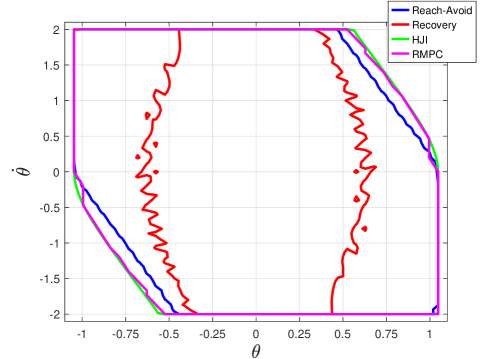
Figure 2: The safe sets for different methods.

The boundary of the feasible states for RMPC [45] is denoted by the magenta line. It almost coincides with the green line (i.e., the boundary of the maximal RIS). This demonstrates the effectiveness of jointly optimizing nominal trajectories and stabilizing controllers on-the-fly, which significantly reduces conservativeness. However, the RMPC approach is much more computationally expensive compared to our proposed safety filter, as shown in Table I (SD denotes standard deviation). Note that the computation time for the three methods in Table I are evaluated on the same computer. The mean computation time of RMPC or its feasibility checking formulation (63) is about 40-50 times larger than the safety filter. It is very challenging for RMPC to realize infeasibility when the system is outside the maximal RIS, so the maximal computation time for RMPC is very large. The feasibility checking formulation performs better, but is still much slower than the safety filter.

TABLE I: Computation Time Comparison

Method	Mean	SD	Max
Proposed safety filter	0.1446 s	0.0225 s	0.2558 s
Nonlinear RMPC from [45]	5.1962 s	7.9486 s	42.1694 s
Feasibility checking for RMPC	4.3684 s	0.5716 s	6.7651 s

VIII Conclusion

In this work, we present a theoretical framework that bridges the advantages of both RMPC and RL to synthesize safety filters for nonlinear systems with state- and action-dependent uncertainty. We decompose the (maximal) RIS into two parts: a target set that aligns with terminal region design of RMPC, and a reach-avoid set that accounts for the rest of RIS. A policy iteration approach is proposed for robust reach-avoid problems and its monotone convergence is proved. This method paves the way for an actor-critic deep RL algorithm, which simultaneously synthesizes a reach-avoid policy network, a disturbance policy network, and a reach-avoid value network. The learned reach-avoid policy network is utilized to generate nominal trajectories for online verification. We formulate a SOCP approach for online verification using system level synthesis, which optimizes for the worst-case reach-avoid value of any possible trajectories. The proposed safety filter requires much lower computational complexity than RMPC and still enjoys persistent robust safety guarantee. The effectiveness of our method is illustrated through a numerical example.

Zeyang Li received the B.S. degree in mechanical engineering in 2021, from the School of Mechanical Engineering, Shanghai Jiao Tong University, Shanghai, China. He is currently working toward the M.S. degree in mechanical engineering with the Department of Mechanical Engineering, Tsinghua University, Beijing, China. His research interests include reinforcement learning and optimal control.

Weiye Zhao is a fifth-year PhD candidate at the Robotics Institute of Carnegie Mellon University, with a primary research focus on providing provable safety guarantees for robots. Specifically, he is interested in safe reinforcement learning, nonconvex optimization, and safe control. He has published in numerous renowned venues, including IJCAI, ACC, CDC, AAAI, CoRL, L4DC, RCIM, LCSS, and others. He serves on the program committee for several conferences, including IV, AAAI, IJCAI, CoRL, CDC, ACC, L4DC, NeurIPS and more.

Chuxiong Hu (Senior Member, IEEE) received his B.S. and Ph.D. degrees in Mechatronic Control Engineering from Zhejiang University, Hangzhou, China, in 2005 and 2010, respectively. He is currently an Associate Professor (tenured) at Department of Mechanical Engineering, Tsinghua University, Beijing, China. From 2007 to 2008, he was a Visiting Scholar in mechanical engineering with Purdue University, West Lafayette, USA. In 2018, he was a Visiting Scholar in mechanical engineering with University of California, Berkeley, CA, USA. His research interests include precision motion control, high-performance multiaxis contouring control, precision mechatronic systems, intelligent learning, adaptive robust control, neural networks, iterative learning control, and robot. Prof. Hu was the recipient of the Best Student Paper Finalist at the 2011 American Control Conference, the 2012 Best Mechatronics Paper Award from the ASME Dynamic Systems and Control Division, the 2013 National 100 Excellent Doctoral Dissertations Nomination Award of China, the 2016 Best Paper in Automation Award, the 2018 Best Paper in AI Award from the IEEE International Conference on Information and Automation, and 2022 Best Paper in Theory from the IEEE/ASME International Conference on Mechatronic, Embedded Systems and Applications. He is now an Associate Editor for the IEEE Transactions on Industrial Informatics and a Technical Editor for the IEEE/ASME Transactions on Mechatronics.

Changliu Liu is an assistant professor in the Robotics Institute, Carnegie Mellon University (CMU), where she leads the Intelligent Control Lab. Prior to joining CMU, Dr. Liu was a postdoc at Stanford Intelligent Systems Laboratory. She received her Ph.D. from University of California at Berkeley and her bachelor degrees from Tsinghua University. Her research interests lie in human-robot collaborations. Her work is recognized by NSF Career Award, Amazon Research Award, and Ford URP Award.

References

- [1] A. D. Ames, S. Coogan, M. Egerstedt, G. Notomista, K. Sreenath, and P. Tabuada, “Control barrier functions: Theory and applications,” in 2019 18th European Control Conference (ECC). IEEE, 2019, pp. 3420–3431.
- [2] Z. Zhao, C. Hu, Z. Wang, S. Wu, Z. Liu, and Y. Zhu, “Back emf-based dynamic position estimation in the whole speed range for precision sensorless control of pmlsm,” IEEE Transactions on Industrial Informatics, 2022.
- [3] S. Lin, C. Hu, S. He, W. Zhao, Z. Wang, and Y. Zhu, “Real-time local greedy search for multi-axis globally time-optimal trajectory,” IEEE Transactions on Systems, Man, and Cybernetics: Systems, 2023.
- [4] R. Zhou, C. Hu, T. Ou, Z. Wang, and Y. Zhu, “Intelligent gru-ric position-loop feedforward compensation control method with application to an ultraprecision motion stage,” IEEE Transactions on Industrial Informatics, 2023.
- [5] C. Liu and M. Tomizuka, “Control in a safe set: Addressing safety in human-robot interactions,” in Dynamic Systems and Control Conference, vol. 46209. American Society of Mechanical Engineers, 2014, p. V003T42A003.
- [6] A. D. Ames, X. Xu, J. W. Grizzle, and P. Tabuada, “Control barrier function based quadratic programs for safety critical systems,” IEEE Transactions on Automatic Control, vol. 62, no. 8, pp. 3861–3876, 2016.
- [7] T. Wei, S. Kang, W. Zhao, and C. Liu, “Persistently feasible robust safe control by safety index synthesis and convex semi-infinite programming,” IEEE Control Systems Letters, vol. 7, pp. 1213–1218, 2022.
- [8] J. Breeden and D. Panagou, “Robust control barrier functions under high relative degree and input constraints for satellite trajectories,” Automatica, vol. 155, p. 111109, 2023.
- [9] K. P. Wabersich, A. J. Taylor, J. J. Choi, K. Sreenath, C. J. Tomlin, A. D. Ames, and M. N. Zeilinger, “Data-driven safety filters: Hamilton-jacobi reachability, control barrier functions, and predictive methods for uncertain systems,” IEEE Control Systems Magazine, vol. 43, no. 5, pp. 137–177, 2023.
- [10] F. Blanchini, S. Miani et al., Set-theoretic methods in control. Springer, 2008, vol. 78.
- [11] I. M. Mitchell, A. M. Bayen, and C. J. Tomlin, “A time-dependent hamilton-jacobi formulation of reachable sets for continuous dynamic games,” IEEE Transactions on Automatic Control, vol. 50, no. 7, pp. 947–957, 2005.
- [12] S. Bansal, M. Chen, S. Herbert, and C. J. Tomlin, “Hamilton-jacobi reachability: A brief overview and recent advances,” in 2017 IEEE 56th Annual Conference on Decision and Control (CDC). IEEE, 2017, pp. 2242–2253.
- [13] J. F. Fisac, A. K. Akametalu, M. N. Zeilinger, S. Kaynama, J. Gillula, and C. J. Tomlin, “A general safety framework for learning-based control in uncertain robotic systems,” IEEE Transactions on Automatic Control, vol. 64, no. 7, pp. 2737–2752, 2018.
- [14] M. Chen, S. L. Herbert, H. Hu, Y. Pu, J. F. Fisac, S. Bansal, S. Han, and C. J. Tomlin, “Fastrack: a modular framework for real-time motion planning and guaranteed safe tracking,” IEEE Transactions on Automatic Control, vol. 66, no. 12, pp. 5861–5876, 2021.
- [15] J. Buch, S.-C. Liao, and P. Seiler, “Robust control barrier functions with sector-bounded uncertainties,” IEEE Control Systems Letters, vol. 6, pp. 1994–1999, 2021.
- [16] Y. Emam, G. Notomista, P. Glotfelter, Z. Kira, and M. Egerstedt, “Safe reinforcement learning using robust control barrier functions,” IEEE Robotics and Automation Letters, no. 99, pp. 1–8, 2022.
- [17] T. Wei, L. Ma, R. Pandya, and C. Liu, “Robust safe control with multi-modal uncertainty,” arXiv preprint arXiv:2309.16830, 2023.
- [18] T. Koller, F. Berkenkamp, M. Turchetta, and A. Krause, “Learning-based model predictive control for safe exploration,” in 2018 IEEE Conference on Decision and Control (CDC). IEEE, 2018, pp. 6059–6066.
- [19] J. Köhler, R. Soloperto, M. A. Müller, and F. Allgöwer, “A computationally efficient robust model predictive control framework for uncertain nonlinear systems,” IEEE Transactions on Automatic Control, vol. 66, no. 2, pp. 794–801, 2020.
- [20] K. P. Wabersich and M. N. Zeilinger, “Linear model predictive safety certification for learning-based control,” in 2018 IEEE Conference on Decision and Control (CDC). IEEE, 2018, pp. 7130–7135.
- [21] A. Georgiou, F. Tahir, I. M. Jaimoukha, and S. A. Evangelou, “Computationally efficient robust model predictive control for uncertain system using causal state-feedback parameterization,” IEEE Transactions on Automatic Control, 2022.
- [22] K. P. Wabersich and M. N. Zeilinger, “A predictive safety filter for learning-based control of constrained nonlinear dynamical systems,” Automatica, vol. 129, p. 109597, 2021.
- [23] S. Liu, C. Liu, and J. Dolan, “Safe control under input limits with neural control barrier functions,” in Conference on Robot Learning. PMLR, 2023, pp. 1970–1980.
- [24] J. Garcıa and F. Fernández, “A comprehensive survey on safe reinforcement learning,” Journal of Machine Learning Research, vol. 16, no. 1, pp. 1437–1480, 2015.
- [25] W. Zhao, T. He, R. Chen, T. Wei, and C. Liu, “State-wise safe reinforcement learning: A survey,” arXiv preprint arXiv:2302.03122, 2023.
- [26] J. Achiam, D. Held, A. Tamar, and P. Abbeel, “Constrained policy optimization,” in International Conference on Machine Learning. PMLR, 2017, pp. 22–31.
- [27] Y. Chow, M. Ghavamzadeh, L. Janson, and M. Pavone, “Risk-constrained reinforcement learning with percentile risk criteria,” The Journal of Machine Learning Research, vol. 18, no. 1, pp. 6070–6120, 2017.
- [28] H. Ma, C. Liu, S. E. Li, S. Zheng, and J. Chen, “Joint synthesis of safety certificate and safe control policy using constrained reinforcement learning,” in Learning for Dynamics and Control Conference. PMLR, 2022, pp. 97–109.
- [29] D. Yu, H. Ma, S. Li, and J. Chen, “Reachability constrained reinforcement learning,” in International Conference on Machine Learning. PMLR, 2022, pp. 25 636–25 655.
- [30] Z. Li, C. Hu, S. E. Li, J. Cheng, and Y. Wang, “Robust safe reinforcement learning under adversarial disturbances,” arXiv preprint arXiv:2310.07207, 2023.
- [31] Z. Qin, K. Zhang, Y. Chen, J. Chen, and C. Fan, “Learning safe multi-agent control with decentralized neural barrier certificates,” in International Conference on Learning Representations, 2021.
- [32] C. Dawson, Z. Qin, S. Gao, and C. Fan, “Safe nonlinear control using robust neural lyapunov-barrier functions,” in Conference on Robot Learning. PMLR, 2022, pp. 1724–1735.
- [33] Y. Wang and X. Xu, “Disturbance observer-based robust control barrier functions,” in 2023 American Control Conference (ACC). IEEE, 2023, pp. 3681–3687.
- [34] A. Leeman, J. Köhler, S. Bennani, and M. Zeilinger, “Predictive safety filter using system level synthesis,” in Learning for Dynamics and Control Conference. PMLR, 2023, pp. 1180–1192.
- [35] O. Bastani, S. Li, and A. Xu, “Safe reinforcement learning via statistical model predictive shielding.” in Robotics: Science and Systems, 2021, pp. 1–13.
- [36] Z. Liu, Z. Guo, Z. Cen, H. Zhang, J. Tan, B. Li, and D. Zhao, “On the robustness of safe reinforcement learning under observational perturbations,” arXiv preprint arXiv:2205.14691, 2022.
- [37] K. Margellos and J. Lygeros, “Hamilton–jacobi formulation for reach–avoid differential games,” IEEE Transactions on Automatic Control, vol. 56, no. 8, pp. 1849–1861, 2011.
- [38] K.-C. Hsu, V. Rubies-Royo, C. J. Tomlin, and J. F. Fisac, “Safety and liveness guarantees through reach-avoid reinforcement learning,” arXiv preprint arXiv:2112.12288, 2021.
- [39] J. Anderson, J. C. Doyle, S. H. Low, and N. Matni, “System level synthesis,” Annual Reviews in Control, vol. 47, pp. 364–393, 2019.
- [40] S. Chen, V. M. Preciado, M. Morari, and N. Matni, “Robust model predictive control with polytopic model uncertainty through system level synthesis,” arXiv preprint arXiv:2203.11375, 2022.
- [41] H. Chen and F. Allgöwer, “A quasi-infinite horizon nonlinear model predictive control scheme with guaranteed stability,” Automatica, vol. 34, no. 10, pp. 1205–1217, 1998.
- [42] M. Althoff, O. Stursberg, and M. Buss, “Reachability analysis of nonlinear systems with uncertain parameters using conservative linearization,” in 2008 47th IEEE Conference on Decision and Control. IEEE, 2008, pp. 4042–4048.
- [43] D. Q. Mayne, “Model predictive control: Recent developments and future promise,” Automatica, vol. 50, no. 12, pp. 2967–2986, 2014.
- [44] A. P. Leeman, J. Köhler, A. Zanelli, S. Bennani, and M. N. Zeilinger, “Robust nonlinear optimal control via system level synthesis,” arXiv preprint arXiv:2301.04943, 2023.
- [45] A. P. Leeman, J. Sieber, S. Bennani, and M. N. Zeilinger, “Robust optimal control for nonlinear systems with parametric uncertainties via system level synthesis,” arXiv preprint arXiv:2304.00752, 2023.
- [46] I. M. Mitchell, “Application of level set methods to control and reachability problems in continuous and hybrid systems,” Ph.D. dissertation, Stanford University, 2002.
- [47] J. A. Andersson, J. Gillis, G. Horn, J. B. Rawlings, and M. Diehl, “Casadi: a software framework for nonlinear optimization and optimal control,” Mathematical Programming Computation, vol. 11, pp. 1–36, 2019.
- [48] T. Haarnoja, A. Zhou, P. Abbeel, and S. Levine, “Soft actor-critic: Off-policy maximum entropy deep reinforcement learning with a stochastic actor,” in International Conference on Machine Learning. PMLR, 2018, pp. 1861–1870.