A Closer Look at Small-Scale Magnetic Flux Ropes in the Solar Wind at 1 AU: Results from Improved Automated Detection

Abstract

Small-scale interplanetary magnetic flux ropes (SMFRs) are similar to ICMEs in magnetic structure, but are smaller and do not exhibit ICME plasma signatures. We present a computationally efficient and GPU-powered version of the single-spacecraft automated SMFR detection algorithm based on the Grad-Shafranov (GS) technique. Our algorithm is capable of processing higher resolution data, eliminates selection bias caused by a fixed $\expectationvalue{B}$ threshold, has improved detection criteria demonstrated to have better results on an MHD simulation, and recovers full 2.5D cross sections using GS reconstruction. We used it to detect 512,152 SMFRs from 27 years (1996 to 2022) of 3-second cadence Wind measurements. Our novel findings are: (1) the radial density of SMFRs at 1 au (${\sim}1$ per $\mathrm{1}\mathrm{0}^{6}\mathrm{k}\mathrm{m}$) and filling factor (${\sim}$35%) are independent of solar activity, distance to the heliospheric current sheet (HCS), and solar wind plasma type, although the minority of SMFRs with diameters greater than ${\sim}$0.01 au have a strong solar activity dependence; (2) SMFR diameters follow a log-normal distribution that peaks below the resolved range ($\gtrsim 10^{4}$ km), although the filling factor is dominated by SMFRs between $10^{5}$ to $10^{6}$ km; (3) most SMFRs at 1 au have strong field-aligned flows like those from PSP measurements; (4) in terms of diameter $d$, SMFR poloidal flux $\propto d^{1.2}$, axial flux $\propto d^{2.0}$, average twist number $\propto d^{-0.8}$, current density $\propto d^{-0.8}$, and helicity $\propto d^{3.2}$. Implications for the origin of SMFRs and switchbacks are briefly discussed. The new algorithm and SMFR dataset are made freely available.

tablenum SIXtablenum

1 Introduction

It is well-known that the solar wind’s magnetic field is only well described by the Parker spiral model on average; at a given point in time, fluctuations deflect the measured magnetic field away from the Parker spiral prediction. Often, the magnetic field fluctuations are correlated with velocity fluctuations, so most early studies viewed them as non-interacting transverse Alfv$\acute{\text{e}}$n waves (e.g. Belcher & Davis (1971)). However, observations showed that solar wind fluctuations, even when Alfv$\acute{\text{e}}$nic, usually exhibit signatures not consistent with pure Alfv$\acute{\text{e}}$n waves, suggesting the presence of nonpropagating structures advected with the rest frame of the solar wind (Burlaga, 1968; Burlaga & Ness, 1968; Burlaga & Ogilvie, 1970; Burlaga & Turner, 1976; Denskat & Burlaga, 1977; Burlaga et al., 1990; Matthaeus et al., 1990). Various theories of solar wind fluctuations consisting of a combination of advected structures and waves were formulated (such as Tu & Marsch (1993)). A popular version of this idea was put forth by Borovsky (2008), wherein the solar wind is considered a sea of magnetic flux tubes that are non-evolving fossil structures originating at the Sun’s surface, or strands of the magnetic carpet. In this picture, flux tubes walls correspond to the observed discontinuities in the solar wind and turbulence is restricted to within the flux tubes. However, an alternative possibility is local generation via magnetohydrodynamic (MHD) turbulence: the cascade of helicity to large scales can form twisted flux ropes in less than the time it takes the solar wind to propagate to 1 au (Matthaeus et al., 2007; Greco et al., 2008; Servidio et al., 2008; Greco et al., 2009; Wan et al., 2009; Zank et al., 2017).

Small-scale magnetic flux ropes (SMFRs) were first reported by Moldwin et al. (1995, 2000), described as transients with magnetic field signatures consistent with flux ropes observed interplanetary coronal mass ejections (ICMEs), but without ICME plasma signatures such as reduced temperature. Various studies have been performed on SMFRs since then, but they were all based on very small lists of events, a few hundred at most. The origin of these structures was debated, with two key possibilities being local reconnection across the heliospheric current sheet (HCS) (Moldwin et al., 2000; Cartwright & Moldwin, 2010) or small CMEs from the Sun (Feng et al., 2008). A significant advancement was made when Zheng et al. (2017) introduced an automated detection algorithm based on the Grad-Shafranov (GS) technique (for a brief overview of the GS technique, which plays an important role in this work, see Appendix A). The detection algorithm was applied to produce a catalog of 74,241 SMFRs over 21 years of Wind measurements (Hu et al. (2018); referred to as the “original catalog”, generated with the “original algorithm”, hereafter).

Considering the large number of SMFRs, are they really transient structures, or are they an essential component of the solar wind? Hu et al. (2018) pointed out that their results were consistent with considering the solar wind as a sea of flux tubes due to the abundance of SMFRs (${\sim}25\%$ of the time is contained in an SMFR in their catalog). Recently, in a systematic study SMFR properties using machine learning, we found that there is essentially no difference between SMFRs and “background” solar wind other than differences imposed by the fixed $\expectationvalue{B}>$5\text{\,}\mathrm{nT}$$ threshold in the original algorithm (Farooki et al. 2023; manuscript submitted to ApJ). Similarly, Zhai et al. (2023) found that the properties of most SMFRs are the same as the properties of the background solar wind. Although these observations suggest that SMFRs are not transients, this is complicated by the observation of a strong solar cycle and HCS proximity dependence for SMFRs in the original catalog, seemingly consistent with the hypotheses of generation via reconnection across the HCS, small CMEs, or even solar eruptions that travel with the HCS as their conduit (Higginson & Lynch, 2018).

Application of the GS-based automated detection algorithm to data from the Parker Solar Probe (PSP) (Chen et al., 2020, 2021; Chen & Hu, 2022) has shown that static SMFRs with low Alfv$\acute{\text{e}}$nicity (correlation between velocity and magnetic field fluctuations) are rare near the Sun compared to 1 au, but including events with high Alfv$\acute{\text{e}}$nicity gives a comparable number. The original detection algorithm excluded Alfv$\acute{\text{e}}$nic events because the GS equation is only valid for magnetostatic structures with no velocity fluctuations (Appendix A) and because torsional Alfv$\acute{\text{e}}$n waves have a similar observational signature to flux ropes, but with high Alfv$\acute{\text{e}}$nicity (Marubashi et al., 2010; Yu et al., 2016; Higginson & Lynch, 2018). However, there have also been observations of Alfv$\acute{\text{e}}$n waves inside SMFRs (Gosling et al., 2010; Shi et al., 2021). In fact, from a theoretical standpoint, there is every reason to expect torsional Alfv$\acute{\text{e}}$n waves to form within flux ropes due to various disturbances (see Gosling et al. (2010) and references therein). Nevertheless, previous 1 au studies based on small event databases did not contain many events with field-aligned flows (Gosling et al., 2010) and only a small percentage of event candidates were excluded due to field-aligned flows in the GS-based original catalog.

We introduce an improved version of the GS-based automated detection algorithm. Our implementation has the following improvements over the original algorithm: (1) we significantly improved the computational efficiency so that supercomputer resources are unneeded and the algorithm can be applied to higher resolution data (we used a consumer-level computer to process 20x higher resolution data than the data processed by supercomputer clusters to generate the original catalog); (2) we incorporated the full GS reconstruction into the detection algorithm to provide more information about the SMFRs and to eliminate the need for the threshold on $\expectationvalue{B}$ to eliminate small fluctuations; (3) we used the generalized GS equation for the case of a field-aligned flow with a constant Wal$\acute{\text{e}}$n slope (as also done by Chen et al. (2021); Chen & Hu (2022) for PSP, but not previously done for Wind). Beyond the new algorithm, we present new findings on the statistical properties of SMFRs. The validity of the statistical findings is strengthened by the improved reliability of the new algorithm, but they are based on a revised analysis, not on the improved reliability of the algorithm.

This paper is structured as follows. Section 2 describes our improved detection algorithm, Section 3 benchmarks the algorithm against simulated measurements, Section 4 describes the data the algorithm was applied to, Section 5 analyzes the size and occurrence of SMFRs, Section 6 analyzes physical properties of the SMFRs, and Section 7 contains discussion and conclusions.

2 Improved Detection Algorithm

2.1 Motivation

The improvements to the algorithm are motivated by a need for increased performance and the need for a better criteria to distinguish small fluctuations and Alfv$\acute{\text{e}}$n waves from SMFRs, discussed below.

2.1.1 Performance

The original detection algorithm is limited by its exhaustive-search nature. That is, it iterates over every possible interval, trying every possible axial orientation. The whole process is then repeated with the smaller sliding window lengths. Even coarse spacing between trial axes, over a hundred trial axes must be used and most calculations must be repeated for each orientation. This is not only inconvenient, but limits the scientific application of the algorithm. The distribution of SMFR durations found in the original catalog continues to increase asymptotically down to the smallest window length used (approximately 10 minutes). Since 21 years of 1-minute cadence data required days of supercomputer time to process, applying the original algorithm to higher cadence data to detect smaller SMFRs would be computationally prohibitive.

2.1.2 Elimination of Small Fluctuations and the Magnetic Field Strength Threshold

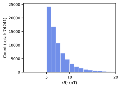
Figure 1: Distribution of $\expectationvalue{B}$ (the magnetic field strength averaged over each flux rope’s interval) in the original catalog.

Since SMFRs were originally considered to be transient structures with elevated magnetic field strength $B$, and the average IMF $B$ is 5 nT, the original algorithm required that $B>$5\text{\,}\mathrm{nT}$$. However, the resulting distribution of $B$ in SMFRs in the original catalog is cut off right at the peak (Figure 1). Therefore, it is likely that ${\sim}$50% of the SMFRs are excluded, which one can expect to cause significant statistical bias. Indeed, as mentioned in the introduction, we have previously demonstrated that the physical properties of SMFRs are mostly the same as the background solar wind other than the fact that $B>$5\text{\,}\mathrm{nT}$$.

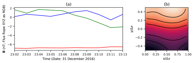
Figure 2: Magnetic field measurements in the flux rope coordinate system (a), as well as the GS reconstruction (b), of event #74238 from the original catalog. In (a), the red, green, and blue lines correspond to $B_{x}$, $B_{y}$, and $B_{z}$, respectively. In (b), the brightness represents $A$. For a flux rope, we expect that $B_{y}$ should exhibit bipolarity and $B_{z}$ should increase towards the center, consistent with the signature observed in (a). Despite that, the GS reconstruction in (b) does not contain any closed transverse field lines.

Is requiring $B>$5\text{\,}\mathrm{nT}$$ an effective method to exclude small fluctuations? Despite this threshold, it appears that the original catalog contains many events that appear to simply be a small fluctuation in the magnetic field direction. We find that an objective way to distinguish small fluctuations from SMFRs is to perform the full GS reconstruction on a given interval to test if it really contains a flux rope (closed transverse field lines in 2D). Figure 2 shows an example. While Figure 2 (a) exhibits a magnetic field signature consistent with the crossing of a flux rope at a high impact parameter, the reconstruction in Figure 2 (b) does not confirm the existence of any closed transverse field lines. It is possible that the event is a flux rope that the spacecraft passed through far from its center, but it could just be a small kink in the magnetic field. The original detection algorithm only tests the hypothesis that each transverse field line is crossed twice. We should also check whether any of those transverse field lines are closed. Using GPUs, it is not computationally prohibitive to perform the GS reconstruction of many sliding windows. As Figure 2 shows, this can eliminate many false positives and thus make the results more reliable.

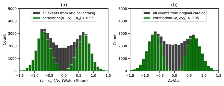
Figure 3: (a) Distribution of Wal$\acute{\text{e}}$n slope calculated using $\mathbf{v}_{\mathrm{HT}}$ for the events original catalog. The histogram is cut off at $\pm 1.5$. Note that for most events, the Wal$\acute{\text{e}}$n slope $\absolutevalue{R_{w}}>0.3$, in contrast to the requirement the original detection algorithm that all events have $\absolutevalue{R_{w}}<0.3$. The green distribution is the subset where the linear correlation is strong, showing that for the events with a well-determined slope, the Wal$\acute{\text{e}}$n slope follows a normal distribution. (b) Same as (a) except using the reference frame agnostic method to determine Alfv$\acute{\text{e}}$nicity as introduced by Chao et al. (2014). In this case, the slope is the relationship between $\derivative*{\mathbf{v}}{t}$ and $\derivative*{\mathbf{v}_{A}}{t}$, which does not depend on the reference frame.

2.1.3 Alfv$\acute{\text{e}}$nicity

We have discovered that the apparent difference in abundance of Alfv$\acute{\text{e}}$nic events between PSP and 1 au is primarily due to a difference in methodology, not a physical difference. The Wal$\acute{\text{e}}$n slope measuring Alfv$\acute{\text{e}}$nicity must be found in the zero electric field frame of reference $\mathbf{v}_{\mathrm{HT}}$ (Appendix A), not in the average velocity frame. But prior to PSP applications, the flux rope velocity $\mathbf{v}_{\mathrm{FR}}$ was approximated as $\expectationvalue{\mathbf{v}}$ instead of $\mathbf{v}_{\mathrm{HT}}$ due to the large volume of data and the computational inefficiency of the original detection algorithm. This has a significant effect on the calculation of the Wal$\acute{\text{e}}$n slope, since the component-by-component Wal$\acute{\text{e}}$n slope must be calculated in the HT frame (Khrabrov & Sonnerup, 1998; Paschmann & Sonnerup, 2008).

The difference between using $\expectationvalue{v}$ and $\mathbf{v}_{\mathrm{HT}}$ can be seen as follows: Suppose that the total bulk velocity is the background velocity plus a fluctuation $\mathbf{v}_{0}+\delta\mathbf{v}$, and that the fluctuation is a field-aligned flow such that it can be written in terms of the Alfv$\acute{\text{e}}$n velocity vector as $\delta\mathbf{v}=R_{w}\mathbf{v_{A}}$, where the constant of proportionality $R_{w}$ is the Wal$\acute{\text{e}}$n slope. If one attempts to evaluate $R_{w}$ using the average velocity frame instead of the HT frame by estimating $\delta\mathbf{v}=\mathbf{v}-\expectationvalue{v}$, an issue arises: this approximation is only valid if $\expectationvalue{\mathbf{v_{A}}}=0$. In a magnetic flux rope, $\expectationvalue{\mathbf{v_{A}}}$ may have a nonzero component in the $\hat{\mathbf{x}}$ direction and always has a significant nonzero component in the $\hat{\mathbf{z}}$ direction (Figure 20). Therefore, the different components will be misaligned, making it impossible to calculate the Wal$\acute{\text{e}}$n slope, in fact resulting in an estimated Wal$\acute{\text{e}}$n slope near zero even for an event with significant field aligned flows.

We calculated the Wal$\acute{\text{e}}$n slope for each event in the original catalog using $\mathbf{v}_{\mathrm{HT}}$ instead of $\expectationvalue{v}$ using the Wind (Wilson et al., 2021) measurements of magnetic field (via the MFI instrument; Lepping et al. (1995)) and plasma moments (via the SWE instruments; Ogilvie et al. (1995)). Figure 3 (a) shows the distribution of the Wal$\acute{\text{e}}$n slope for the events in the original catalog. Even though the original algorithm excludes events with $\absolutevalue{R_{w}}>0.3$, less than 25% of the events actually meet that threshold when $\mathbf{v}_{\mathrm{HT}}$ is used to calculate the Wal$\acute{\text{e}}$n slope.

One might wonder if $\mathbf{v}_{\mathrm{HT}}$ artificially introduces the field-aligned flow by minimizing $\mathbf{v}\crossproduct\mathbf{B}$. Figure 3 (b) shows the same result using a reference-frame independent method to determine Alfv$\acute{\text{e}}$nicity (Chao et al., 2014): instead of taking the slope of $\delta\mathbf{v}\propto\mathbf{v}_{A}$, one can take the derivative of both sides and then the slope can be evaluated in any reference frame. The result using the frame-independent method is the same as the result obtained using the HT frame: most events in the original catalog at 1 au are highly Alfv$\acute{\text{e}}$nic.

2.2 Optimization

An easy way to optimize the detection algorithm is to take advantage of the fact that the same computations are applied to each interval. In Python, loops are slow. This problem can be avoided by processing multiple intervals simultaneously via matrix computations. On a CPU, this benefit is a consequence of the limitation of the Python language. However, GPUs can take greater advantage of this, because unlike CPUs, they apply a single instruction to large arrays in parallel. In our implementation, we utilize batch processing and run our code on a GPU using the PyTorch software package for matrix computations. The interpolation operation necessary for the computation of $R_{\mathrm{diff}}$ is made possible by using another software package (https://github.com/aliutkus/torchinterp1d). The use of GPU processing allows our implementation to process large volumes of data on a consumer-grade computer instead of a supercomputer.

We further improved the performance of the algorithm by reducing the search space for axial orientation $\hat{\mathbf{z}}$ (Figure 20). This is possible due to the following realization. For an acceptable flux rope interval, the same field line is observed at the beginning and end. Since the poloidal flux function $A$ is a field line invariant, the final $A$ equals the last $A$, that is, $A_{f}=A_{0}$. Since the difference in $A$ is given by integrating $B_{y}$ (Appendix A), the integral of $B_{y}$ over the interval must then be zero. Therefore, the average magnetic field vector must be perpendicular to $\hat{\mathbf{y}}$, since $\expectationvalue{\mathbf{B}}\dotproduct\hat{\mathbf{y}}=\expectationvalue{\mathbf{B}\dotproduct\hat{\mathbf{y}}}=-\absolutevalue{v_{x}}\int_{t_{0}}^{t_{0}+\Delta t}B_{y}dt/\Delta t=0$ (where the average $\expectationvalue{\mathbf{B}}$ must be calculated as the integral of each component over the interval divided by the length, rather than the mean of each component).

So $\expectationvalue{\mathbf{B}}$ is perpendicular to $\hat{\mathbf{y}}$, in addition to $\mathbf{v}_{\mathrm{FR}}$ (following from the definition of the vertical direction $\hat{\mathbf{y}}$; Figure 20). Then, even before knowing $\hat{\mathbf{z}}$, $\pm\hat{\mathbf{y}}$ is already determined. This explains why the uncertainty in $\hat{\mathbf{z}}$, often referred to as azimuthal uncertainty when viewed in the GSE coordinate system, is typically much greater than the uncertainty in $\hat{\mathbf{y}}$, as observed by Hu & Sonnerup (2002). Once $\pm\hat{\mathbf{y}}$ is known, $A$ is known up to a constant factor of $\pm v_{x}$. However, for the purpose of finding $\hat{\mathbf{z}}$, only the relative values of $A$ are needed to specify the field line corresponding to each measurement, so we can simply normalize $A$ to start at $0$ and peak at $1$.

To find $\hat{\mathbf{z}}$, we still need to minimize the difference residue $R_{\mathrm{diff}}(\theta)$ (Appendix A) where $\theta$ is the angle between $\hat{\mathbf{z}}$ and $\mathbf{v}_{\mathrm{FR}}$ about $\hat{\mathbf{y}}$. The only component of $P_{t}$ affected by the choice of $\theta$ is $B_{z}^{2}/2\mu_{0}$, so we only need to minimize the contribution from the $B_{z}$ term (and $B_{z}$ itself is a field line invariant; Appendix A). Originally, we would have to calculate $B_{z}(t)=\mathbf{B}(t)\dotproduct\hat{\mathbf{z}}$ for each $\hat{\mathbf{z}}$, then linearly interpolate the values before and after the peak $A$ onto $A(t)$, yielding $B_{z}^{(1)}(A)$ and $B_{z}^{(2)}(A)$. Finally, we would calculate $R_{\mathrm{diff}}=\sqrt{\expectationvalue{(B_{z}^{(2)}(A)-B_{z}^{(1)}(A))^{2}}}/(\max(B_{z})-\min(B_{z}))$ for each $\theta$. However, linear interpolation is a fairly expensive operation. Instead of performing it each time, we can take advantage of the fact that the normalized $A$ is fixed and is not affected by $\theta$, so the linear interpolation for each point is just a linear combination of the original values of $B_{z}$ with coefficients independent of $\theta$ or $\hat{\mathbf{z}}$. So if instead we interpolate the vector $\mathbf{B}$ by interpolating its components, we can construct an $N\times 3$ matrix of difference vectors $\mathbf{B}^{(2)}(A)-\mathbf{B}^{(1)}(A)$, where $N$ is the number of measurements. If we multiply it by the $3\times M$ matrix of $M$ possible $\hat{\mathbf{z}}$ orientations, each element of the resulting $N\times M$ matrix is $B_{z}^{(2)}(A)-B_{z}^{(1)}(A)$ for the measurement corresponding to the row and the possible $\hat{\mathbf{z}}$ corresponding to the column. Squaring the values of the matrix and summing over the rows yields the numerators for calculating $R_{\mathrm{diff}}(\theta)$. From there, the same procedure can be applied to the original $N\times 3$ matrix of measured magnetic field vectors $\mathbf{B}$ to obtain $B_{z}(t)$ for each orientation, which can then be used to find $\max(B_{z})-\min(B_{z})$ and thus the denominator of $R_{\mathrm{diff}}$.

The procedure outlined above makes the assumption that the interval is perfectly selected and does not need to be trimmed further. Making the first assumption requires the use of very narrowly spaced sliding window lengths. For example, Hu et al. (2018) used 1-minute cadence data with sliding windows 5 minutes apart in length, trimming the window to be shorter if necessary. With this new procedure, a 1-minute separation between window lengths would be necessary due to the assumption that the interval is already trimmemd. However, this only requires visiting each flux rope candidate at most five additional times, whereas the reduction by finding $\hat{\mathbf{y}}$ first is significantly greater.

Another assumption made is that $\mathbf{v}_{\mathrm{FR}}\crossproduct\expectationvalue{\mathbf{B}}\neq 0$. When this relationship is not satisfied, we need to resort to a full trial-and-error process. We do this by trying every possible $\hat{\mathbf{y}}$ (with 1 degree spacing) and finding the one that has a single stationary point, the absolute value of the last $A$ value being less than 10% of the absolute value of the peak $A$, and that minimizes $R_{\mathrm{diff}}$ when $\hat{\mathbf{y}}$ is not well specified. We evaluate $\hat{\mathbf{y}}$ as being well-specified by taking the cross product of the estimated $\hat{\mathbf{y}}$ and $\mathbf{v}_{\mathrm{FR}}$, and validating the average magnetic field along this perpendicular direction is not less than 10% of the average of the magnetic field magnitude. The handling of this edge case is not particularly important and only introduces a minimal performance impact, since the average magnetic field direction being parallel to the velocity is rare (even near the Sun, where the magnetic field is approximately radial, the Parker Solar Probe’s own motion perpendicular to the radial direction ensures that the velocity relative to the spacecraft is not purely radial).

The new procedure for finding the axial orientation provides a substational improvement in the performance of the algorithm. Additionally, it makes it easy to increase the angular precision from more than 10 degrees to less than 1 degree without an absurd computational cost, since the search for $\hat{\mathbf{z}}$ is now reduced to varying 1 angular parameter instead of every combination of two angular parameters. For example, if both the azimuthal and latitudinal separations were 1 degree, over 30,000 trial axes would be necessary for every interval.

Figure 4: Flow chart describing the improved detection algorithm.

2.3 Algorithm

In this section, we describe the algorithm step by step for reproducibility purposes. The overall procedure is outlined in Figure 4. Essentially, the algorithm checks every single interval for a set of interval lengths, tests whether the interval is compatible with a flux rope signature: (1) magnetostatic or MHD equilibrium is validated by finding and validating $\mathbf{v}_{\mathrm{HT}}$; (2) smoothness of the magnetic field in the interval at the given scale is tested by comparing the raw measurements to a smoothed version of the measurements; (3) the optimal 2D orientation is found and the hypothesis of a 2D structure where every field line is crossed twice is tested by verifying that $A$ that $P_{t}^{\prime}=P_{t}^{\prime}(A)$; (4) the structure is checked for closed field lines via GS reconstruction; (5) the remaining sliding windows are filtered to avoid overlap, giving preference to larger event candidates over smaller ones.

2.3.1 Selecting Smooth Intervals Exhibiting MHD Equilibrium

First, we process the data using a set of sliding windows. Our goal is to use window lengths that span multiple orders of magnitude, and GPUs have limited memory, so some additional steps are required. We set a maximum processing resolution $N_{\mathrm{max}}$. If the sliding window length $N_{\mathrm{window}}>N_{\mathrm{max}}$, then we must downsample the data so that the windows are not prohibitively memory intensive. For example, using 3 second cadence data, a window length approximately equal to 3 days would contain approximately $10^{5}$ data points. We find that $N_{\mathrm{max}}=64$ does not significantly affect the results compared to higher resolutions despite providing a substantial performance gain. To downsample the data, we first perform a boxcar average with both length and step size set to $\lfloor N/N_{\mathrm{max}}\rfloor$, so that the remaining downsampling factor is less than a factor of 2. Then, we use linear interpolation to resample the data so that the window length becomes $N=N_{\mathrm{max}}$. If $N<N_{\mathrm{max}}$, then the window length is left as is. To ensure that the event’s magnetic field fluctuation is “smooth” so that the downsampling and smoothing employed throughout the algorithms is valid, we require that the average cosine angle between the downsampled vectors and their moving average with kernel size $\lfloor N/10\rfloor$ (rounded up to the nearest odd number if even) be at least 0.98.

Next, we evaluate $\mathbf{v}_{\mathrm{HT}}$ and the average $\mathbf{B}$ (using the trapezoid rule since the same is used for evaluating the poloidal flux function $A$) for each sliding window. Using these quantities, we evaluate the vertical direction $\hat{\mathbf{y}}$. The correlation coefficient for $\mathbf{v}_{\mathrm{HT}}$ (Khrabrov & Sonnerup, 1998) is required to be at least 0.95, and $B_{y}$ is required to have exactly one change of sign after (applying the same filter used for the smoothness check to avoid excluding events containing embedded fluctuations).

2.3.2 Finding 2D Orientation and Validation of 2D Hypothesis

For the sliding windows that remain, we evaluate the minimum residue $\hat{\mathbf{z}}$ with 256 trial axes centered around the direction of the average magnetic field uniformly spread between $\pm$90\text{\,}\mathrm{\SIUnitSymbolDegree}$$ about the estimated $\hat{\mathbf{y}}$. The selected $\hat{\mathbf{z}}$ is guaranteed to result in a trimmed $A$, as it is perpendicular to the already estimated $\hat{\mathbf{y}}$. The resolution n of the distinction between $\hat{\mathbf{x}}$ and $\hat{\mathbf{z}}$ is $$180\text{\,}\mathrm{\SIUnitSymbolDegree}$/256\approx$0.7\text{\,}\mathrm{\SIUnitSymbolDegree}$$, but our benchmarking suggests that the actual uncertainty is on the order of $10\text{\,}\mathrm{\SIUnitSymbolDegree}$. We require $R_{\mathrm{diff}}<0.3$ (Appendix A) separately for $B_{z}$ and $P_{t}$. Previous GS-based detection studies used a stricter threshold for $R_{\mathrm{diff}}$ since they did not directly solve the GS equation to validate the flux rope structure and relied primarily on a low $R_{\mathrm{diff}}$ for detection. However, many events studied using GS reconstruction in the literature had significantly higher values of $R_{\mathrm{diff}}$, and even flux ropes in MHD simulations can have higher $R_{\mathrm{diff}}$. We find that in conjunction with our validation through GS reconstruction, a threshold of 0.3 provides satisfactory results. Note that we do not use the extra factor of $1/\sqrt{2}$ in our definition of $R_{\mathrm{diff}}$, which would make our threshold just over 0.2 by the definition used in Hu et al. (2018).

Since it seems that most SMFRs have non-negligible Alfv$\acute{\text{e}}$nicity (Figure 3), we must account for the Alfv$\acute{\text{e}}$nicity when calculating the generalized transverse pressure $P_{t}$. We use the Wal$\acute{\text{e}}$n slope to estimate a constant Alfv$\acute{\text{e}}$n Mach number in the flux rope frame of reference $M_{A}$, so that we may use Equation A2 to calculate the generalized $P_{t}$. When the Wal$\acute{\text{e}}$n slope is greater than 0.3, we require that the correlation coefficient between $\mathbf{v}-\mathbf{v}_{\mathrm{HT}}$ and $\mathbf{v}_{A}$ be at least 0.8, and we exclude events with a Wal$\acute{\text{e}}$n slope greater than 0.9 to avoid a singularity in Equation A2 (Chen et al., 2021; Chen & Hu, 2022).

2.3.3 Full GS Reconstruction

We perform the full GS reconstruction for all of the sliding windows that pass the above tests. (Sonnerup et al., 2006; Teh, 2018). The settings must work well when applied to a large number of events automatically without any manual adjustments. This is especially important due to the sensitivity of solving the GS equation as an initial value problem. Based on our experimentation, we find that it is suitable to use a third-order polynomial to fit $P_{t}(A)$ and take its derivative to derive the current density used for the reconstruction. The validity of the polynomial fit is ensured by requiring the events to have $R_{\mathrm{fit}}$ no more than 0.3. Additionally, we require that the axial current density increases towards the center of the closed region, since real flux ropes carry strong axial currents that are strongest at their center. We added this requirement because SMFRs should carry strong axial currents to generate their poloidal magnetic field, and because in the MHD simulation we benchmarked the algorithm on, all events where the reconstruction did have a monotonically increasing current density were false positives.

The size of the reconstruction domain is fixed at 11x11 pixels with step size $\Delta y=0.1\Delta x$, and we use the standard three-point smoothing introduced in (Hau & Sonnerup, 1999) for the stability of the numerical integration. The 1D measurements are downsampled to 11 data points and the reconstructed cross section is 11x11 pixels (5 pixels above and below the spacecraft path). For values of $A$ outside of the measured range, the lower tail of $P_{t}(A)$ is extrapolated using a decaying exponential so that the current density decays outside of the measured field lines, while for the upper tail, it is simply allowed to continue according to the polynomial fit. Once the reconstructed map is obtained, events without a core with closed transverse field lines according to the procedure previously mentioned are excluded. We also require that the closed region be more than 4 pixels wide and 4 pixels tall and that it overlap with the strip measured by the spacecraft. The procedure for finding the core region is described in Appendix B.

2.3.4 Cleanup of Overlapping Windows

Once the candidate windows are obtained for a given sliding window size, we follow the same procedure as in the original algorithm: For a given window length, we use the greedy algorithm to remove overlapping events. However, rather than prioritizing events by their end time, we prioritize them by $R_{\mathrm{diff}}$. The gaps between larger events are filled with events detected from smaller sliding window sizes, but larger events are prioritized over smaller events.

3 Benchmarking Against Simulated Measurements

3.1 Small Fluctuations

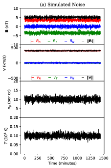
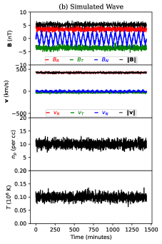
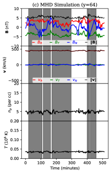
Figure 5: Examples of the results on simulated timeseries. Intervals detected as flux ropes are shaded. The columns are: (a) background field plus noise (b) background field plus pure Alfv$\acute{\text{e}}$n wave (c) MHD simulation

Since the number of events detected is so large and most of them are quite short, one could reasonably be concerned that a significant portion of the detected events are not flux ropes at all, but rather small fluctuations, such as noise or waves. Here, we demonstrate that such fluctuations are not a significant source of false positives.

First, we generate simulated, noisy data. All vector quantities here are in radial-tangential-normal (RTN) coordinates. We generate 1 day of 1 minute cadence simulated data. The magnetic field data is a constant Parker spiral aligned field plus Gaussian noise $\boldsymbol{\mathcal{N}}$ with mean $\mu$ and standard deviation $\sigma$: $\mathbf{B}=$5\text{\,}\mathrm{nT}$(\sqrt{2}\hat{\mathbf{R}}-\sqrt{2}\hat{\mathbf{T}})+\boldsymbol{\mathcal{N}}(\mu=0,\sigma=$0.5\text{\,}\mathrm{nT}$)$. The proton number density $n_{p}=\mathcal{N}(\mu=$10\text{\,}\mathrm{c}\mathrm{m}^{-3}$,\sigma=$1\text{\,}\mathrm{/}\mathrm{c}\mathrm{m}^{-3}$)$, the proton temperature $T=\mathcal{N}(\mu=$1\text{\times}{10}^{5}\text{\,}\mathrm{K}$,\sigma=$1\text{\times}{10}^{4}\text{\,}\mathrm{K}$)$, and the proton bulk velocity is radial plus noise $v=$400\text{\,}\mathrm{km}\text{\,}{\mathrm{s}}^{-1}$\hat{\mathbf{R}}+\boldsymbol{\mathcal{N}}(\mu=0,\sigma=$10\text{\,}\mathrm{km}\text{\,}{\mathrm{s}}^{-1}$)$. The data is plotted in Figure 5 (a). Additionally, we generate a similar artificial data interval with a simple Alfv$\acute{\text{e}}$n wave added: $\mathbf{B}\to\mathbf{B}+\sin((2\pi/$60\text{\,}\mathrm{min}$)t)\hat{\mathbf{N}}$ and $\mathbf{v}\to\mathbf{v}+\mathbf{v}_{A}$. The data with the wave is plotted in Figure 5 (b).

As expected, neither the noisy simulated data nor the wavy simulated data had any flux ropes detected with windows ranging from 10 to 360 minutes. Though we did not reproduce it here, after many repetitions with a higher $\sigma$ for the magnetic field noise, we managed to get one single event of only 10 data points to be detected. However, that is far too rare to explain the large number of SMFRs that are detected in a given day of real data. Also not shown here, we have verified that even with the velocity fluctuations in the simulated data removed or with a magnitude lower than the Alfv$\acute{\text{e}}$n speed, the simulated wave is not detected as an event by our algorithm. Thus, noise and pure transverse Alfv$\acute{\text{e}}$n waves are not likely to be a significant source of false positives.

3.2 MHD Simulation

To validate the applicability of our method to realistic SMFRs, we tested our new algorithm on SMFRs generated from a 2.5D MHD turbulence simulation.

We test our algorithm in numerical simulations of compressible MHD (CMHD). The CMHD equations are solved in a $2.5$D square box of length $2\pi L_{0}$ in either direction, with 4096 points per side, using a pseudo-spectral code as described in Ref. (Vásconez et al., 2015; Perri et al., 2017; Pecora et al., 2021). The simulation was performed in the $x$-$y$ plane with a mean magnetic field $B_{0}=1$ along the $z$ direction. Velocity and magnetic field fluctuations have all three Cartesian components. The algorithm is stabilized by fourth-order hyperviscosity that suppresses very small-scale, numerical effects. The parameters of the simulation are appropriate to describe solar wind conditions, magnetic fluctuations are such that $\delta b/B_{0}=1/2$ and plasma $\beta\sim 0.5$, with $\delta b$ total r.m.s magnetic fluctuation amplitude and $\beta$ ratio of kinetic to magnetic pressures. The initial fluctuations are chosen with random phases, for both magnetic and velocity fields, in a shell of Fourier modes with $3\leq|{\boldsymbol{k}}|\leq 5$. The decaying CMHD simulation quickly develops turbulence and small-scale dissipative structures. The magnetic field power spectrum (not shown here) manifests a typical scaling $P(k)\propto k^{-5/3}$. The turbulent pattern is represented in Figure 6.

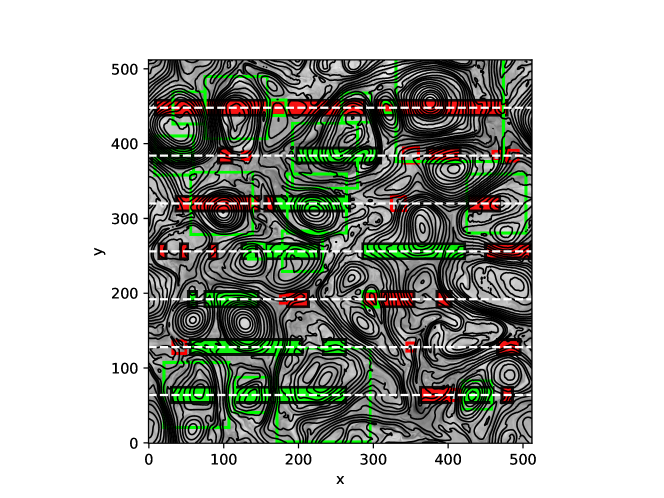
Figure 6: Results from applying the improved algorithm to a 2.5D MHD turbulence simulation. The brightness represents the strength of $B_{z}$ and the blue streamlines represent the transverse field lines. The dashed lines are virtual spacecraft paths through the simulation. The square boxes represent sliding window intervals that were detected as flux ropes by the new algorithm. The rectangular boxes represent the intervals detected as events by the original algorithm. Green boxes are classified as true positives, whereas red boxes are classified as false positives.

Table 1: Quantitative comparison between both algorithms when applied to the MHD simulation and with or without events below 30 data points.

Algorithm	Time per row	True Positive (TP)	TP ($N>30$)	Good Reconstruction (Rec)	Rec ($N>30$)
Original	${\sim}4$m	14 (42%)	12 (57%)	N/A	N/A
New	${\sim}2$s	18 (64%)	14 (100%)	35%	79%

Figure 6 shows the results of applying the detection algorithm to the MHD simulation (downsampled to 512x512). Virtual spacecraft were sent through several paths to take virtual measurements, to which the detection algorithm was applied. An example for a single spacecraft path is shown in Figure 5 (c). Also included are rectangles representing events detected using the original algorithm. We automatically classify a detected event as a true positive if (1) the interval has a closed field line and (2) the true $B_{y}$ has only one inflection point (after smoothing). True positives are labeled green while false positives are labeled red.

Although the original algorithm occasionally picks up good events that the new algorithm misses, in many cases it either incorrectly combines multiple events into one, or it detects some fluctuations at the boundary or within a flux rope. In contrast, the new algorithm usually identifies the flux rope correctly, even if it does not have an accurate reconstruction. However, for the smallest window sizes with less than 30 data points, even the new algorithm picks up some none-flux rope fluctuations as SMFRs. Quantitative comparison is provided in Table 1. From this comparison, it is clear that the new algorithm is both significantly faster than the original algorithm and significantly more reliable.

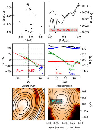
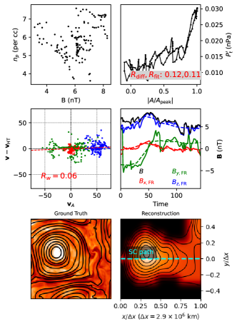
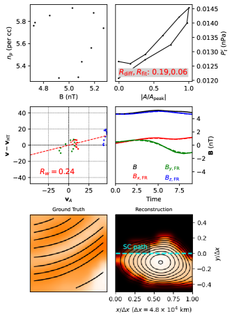
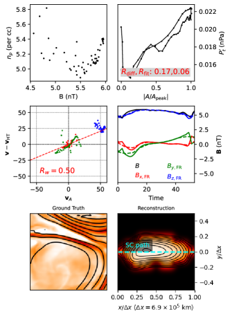
Figure 7: Four events detected by virtual spacecraft from the MHD simulation. Top left: Relation between $B$ and $n_{p}$. Top right: $P_{t}^{\prime}$ as a function of $A$ (Appendix A). Center left: Relationship between Alfv$\acute{\text{e}}$n velocity (as a vector) and the velocity fluctuations. Center right: Measured magnetic field components and strength (solid lines) and model magnetic field components (dashed lines) in the flux rope coordinate system. Bottom: Reconstructed cross section with contours at equally spaced values of the flux function $A$ (in the estimated flux rope coordinate system), along with the ground truth magnetic field (in the simulation coordinate system, not the estimated flux rope coordinate system).

Manual comparison between the reconstructed cross sections and the true magnetic field geometry suggests that the algorithm reliably detects the presence of flux ropes (86% of the time). However, the reconstruction is only reliable 35% of the time. This appears to be because when the spacecraft crosses the flux rope close to the edge, the wrong boundaries are selected, so the reconstruction is inaccurate even though there is excellent agreement with the spacecraft measurements over the 1D path that it crossed. It is not possible to consistently distinguish which reconstructions are reliable because even the cases with an accurate reconstruction can exhibit a relatively high $R_{\mathrm{diff}}$, whereas the reconstructions that are way off can sometimes have a low $R_{\mathrm{diff}}$. Therefore, for additional validation of the reconstruction, it would be valuable to incorporate multi-spacecraft analysis in future studies. For the purposes of this study, due to the focus on the long-term trend, we must work within the limitation of single spacecraft measurements. Even when the reconstructed geometry is inaccurate, the order of magnitude of estimated parameters such as size and current density are usually reliable.

It is worth noting that, at least for this simulation, the large events (greater than 30 data points) tend to be reliable, wheras the small events (less than 30 data points) tend to be unreliable. However, this may be due in part to the scale of the flux ropes in the simulation being larger to begin with. This is because it is easier to randomly satisfy a false hypothesis with a small number of data points, but events with many data points can usually be more reliably validated.

In Figure 7, we show the detection algorithm’s output for four example events based on the simulated data. The top two events are “good” results, whereas the bottom two are “bad” results. In all four cases, the algorithm correctly identified a flux rope, but in the “bad” cases, the reconstruction is inaccurate. Unfortunately, we have not been able to find any criteria that can consistently evaluate the reliability of a reconstruction. For example, the bottom events have lower $R_{\mathrm{diff}}$ than the top left event. Setting a lower threshold on $R_{\mathrm{diff}}$ does not appear to improve the quality of the events overall. In most cases, bad events are very small (less than 30 data points), but there are exceptions (such as the event on the bottom right of Figure 7). Bad events tend to have a highly inaccurate $\hat{\mathbf{z}}$, but of course there is no way to know that without the ground truth. This highlights the limitation of single-spacecraft measurements: Even when measuring a perfectly time-static and 2D plasma, the spacecraft cannot determine the true $\hat{\mathbf{z}}$ and $A$. It can only test whether a given interval satisfies the hypothesis of being 2D and having an $A$ with a single stationary point given a certain $\hat{\mathbf{z}}$ by checking if certain necessary conditions are approximately met. Without a measurement of the magnetic field gradient, there are no sufficient conditions. Additional context may be gained by comparing the event’s measurements to the surrounding measurements, which is a potential area of future research to improve single-spacecraft SMFR detection.

4 Application to Wind Data

We applied our new algorithm, described in Section 2, to 27 years of Wind data (Wilson et al., 2021) from years 1996-2022. Each year was processed separately. For magnetic field measurements, we used the Magnetic Fields Instrument (MFI; Lepping et al. (1995)) 3-second vector magnetic field measurements. For measurements of the bulk plasma parameters, we used the proton moments from the 3DP instrument (Lin et al., 1995) computed on-board at a 3-second cadence. To calculate gas pressure $p$ and Alfv$\acute{\text{e}}$n speed $v_{A}$, we only included the proton contribution due to the lack of continuously available quality electron and alpha particle moments. We used linear interpolation to bring the two datasets onto a set of consistently spaced points, allowing for a maximum of a 6-second gap between the points used for interpolation. Points where missing values existed were recorded and then the remaining gaps were filled using linear interpolation. A number density less than 1 per cc was considered missing, since the quality of the plasma measurements is poor when the measured number density is very low.

The 3DP measurements appear to occasionally have massive spikes, so before interpolating each property onto the consistently spaced points, we applied a spike removal algorithm based on Roberts (1993). Each point in a 100-point window is marked bad if it is distanced from the mean of the window by more than six standard deviations. We repeat this twice rather than iteratively processing each window as done by Roberts (1993) to simplify the algorithm and make it possible to compute in parallel. Additionally, due to limited telemetry, there is some digitization effect present in the 3DP data which introduces sudden jumps to the data. To alleviate that, we applied a 5-point running average to the plasma parameters.

After preparing the dataset, we applied the detection algorithm with 195 logarithmically spaced sliding windows from $10$ (30 seconds) to $10^{5}$ data points (approximately 3.5 days). The largest window sizes are just for thoroughness: the important range is up to $10^{5}$ seconds (order of days), since that is the typical order of magnitude of CME durations at 1 au. We do not expect to see SMFRs larger than CMEs. A total of 594,857 events were detected, but after restricting the list to only those with fewer than 10% of the interval containing missing values, 512,152 remained.

Despite the large volume of high-resolution data, our implementation was able to process each year of data in only about a few minutes on a consumer-level GPU (Nvidia GeForce RTX 3090). Most of the time is spent on the GS reconstruction, without which a year of data can be processed in less than a minute. The high-performance implementation with GPU acceleration made it possible to do much more than could be easily done with the original implementation. We did not use any supercomputer resources and the improved algorithm also provides GS reconstructions.

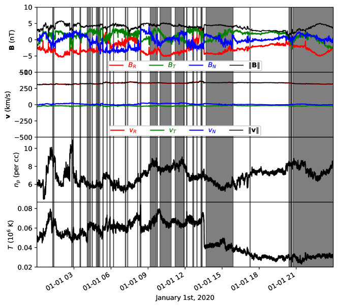
Figure 8: Example of input measurements for a single day, with event intervals shaded gray.

Figure 8 displays an example of the data used for detection for a single day. This figure is representative of typical quiet solar wind conditions. Although on average, the magnetic field is aligned with the Parker spiral, there are usually significant rotations in the magnetic field direction. Nearly half of the total time is detected as a flux rope. Unlike ICMEs, most of the flux ropes do not have extremely high magnetic field strength, nor do they necessarily have decreased proton temperature, nor do they appear to have any expansion signature (as the velocity does not change much). The sizes of the SMFRs vary significantly, ranging from less than a minute to more than an hour. The larger ones are less frequent but occupy a significant portion of the total time; the smaller ones occur in larger numbers but don’t compose the majority of the solar wind.

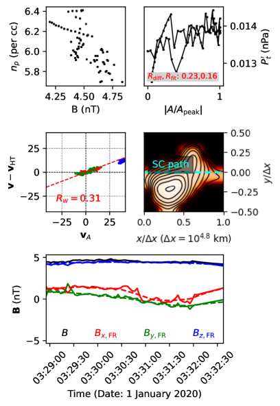
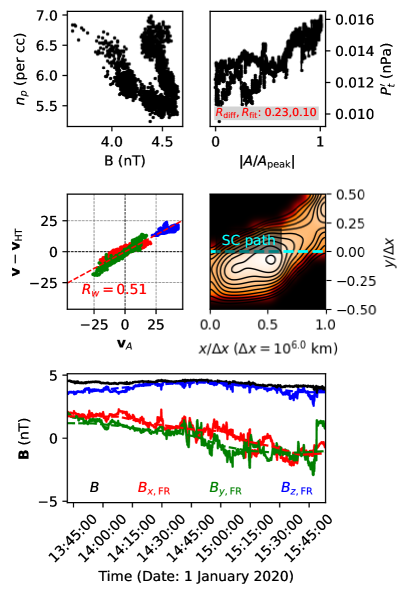
Figure 9: Two examples of real events detecting from Wind data. The first event (left) is a relatively small event while the second event (right) is a relative large event. Top left: Relation between $B$ and $n_{p}$. Top right: $P_{t}^{\prime}$ as a function of $A$ (Appendix A). Center left: Relationship between Alfv$\acute{\text{e}}$n velocity (as a vector) and the velocity fluctuations. Center right: Reconstructed cross section with contours at equally spaced values of the flux function $A$. Bottom: Measured magnetic field components and strength (solid lines) and model magnetic field components (dashed lines) in the flux rope coordinate system.

Figure 9 shows two examples outputs from our detected algorithm (one small, one large). Note that both events have $|R_{w}|>0.3$, but are inconsistent with an interpretation of them as Alfv$\acute{\text{e}}$n waves due to the nonzero change in $B_{z}$ and the anticorrelation between $B$ and $n_{p}$ (Vellante & Lazarus, 1987). The effect in the field aligned flow can be seen in the green points in the velocity scatter plot, which change sign along with $B_{y}$. Even though $R_{\mathrm{diff}}$ and $R_{\mathrm{fit}}$ are high compared to the thresholds used by previous studies, the model fits the data very well. The reconstructed cross section shows that GS reconstruction applied to the measurements reveals closed transverse field lines, validating the flux rope nature of the events. Unlike CMEs, neither the small event (about 3 minutes long) nor the long event (about 2 hours long) have an elevated magnetic field strength. However, many of the detected events do have large changes in the field strength, although most do not exhibit other signatures of CMEs such as velocity expansion signature or very low temperatures. It seems that the change of magnetic field strength depends on the geometry of the flux rope. Unlike CMEs, SMFRs do not need large changes in magnetic field strength because they are usually not force-free.

In the following sections, we statistically analyze various aspects of the new database of events. For additional context, we used the classification scheme introduced by Xu & Borovsky (2015) to distinguish SMFRs in ejecta, sector reversal, streamer belt origin, and coronal hole origin plasma streams. Since the plasma quantities in Xu & Borovsky (2015) are calibrated for 1 hour averaged OMNI2 data, which is primarily based on Wind’s Faraday cup instrument SWE, we evaluated the solar wind classification based on SWE data downsampled to 1 hour, then evaluated each event’s classification as the the nearest hourly classification.

5 SMFR Size and Occurrence

5.1 Size Distribution

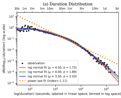
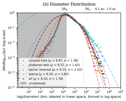
Figure 10: (a) Histogram of the duration (represented as a scatter plot to comparing with the fitted curves). Each black point in the scatter plot represents the number of events detected for a particular sliding window scaled by the bin separation to make it represent the estimated probability density. The points in the scatter plot are centered at the geometric mean of the corresponding window size and the window size after it so that it is centered between the two values in log space. The three curves are log-normal distribution fits with different values of $\mu$. Note that $\mu$ and $\sigma$ are location and scale parameters for the log-normal distribution, not the mean and standard deviation. They are defined so that the natural logarithm of a log-normal distribution is normally distributed with mean $\mu$ and standard deviation $\sigma$. The pink line is a power law fit to the range between 10 minutes and 6 hours. (b) Diameter distribution following the same format as (a). The shaded region covers diameters that are below $($600\text{\,}\mathrm{km}\text{\,}{\mathrm{s}}^{-1}$)($30\text{\,}\mathrm{s}$)$. Flux ropes with diameters below this cutoff and orientations perpendicular to the radial direction can be too short for the smallest sliding window. The distribution for each solar wind type is also plotted separately with its own fit.

Figure 10 (a) displays the distribution of the duration of the detected events. Over the range from 10 minutes to 6 hours, it appears to exhibit a power law similar to the result in the original catalog. However, with the added orders of magnitude, a deviation from a simple power law becomes apparent, and there is significant curvature. Looking closely at the power law portion of the distribution from our figure as well as the figures in in (Hu et al., 2018), there is already a slight curvature even for the limited range. Our expanded range of durations makes the deviation of the power law obvious. Log-normal distributions are very common in nature and in the solar wind. It is very common for a log-normal distribution to be mistaken for a power law distribution when viewed over a limited range. This motivates fitting the data to a log-normal distribution, which we demonstrate in Figure 10 (a). Clearly, the log-normal distribution provides a superior fit. However, the peak of the distribution is below 30s, the smallest sliding window used in the detection process. Therefore, the distribution is not fully resolved. Moreover, a fit of similar quality is attained for an arbitrary choice of the peak as shown in Figure 10 (a). Therefore, we cannot determine the exact parameters of the log-normal distribution. Still, a log-normal distribution clearly fits the data very well over the resolved range.

The only significant deviation from log-normal in Figure 10 (a) appears to be a discontinuity around 1 minute. Considering that 1 minute and 30 seconds corresponds to 30 data points, this may be a consequence of the unreliability of SMFRs detected from such a small number of data points. The distribution appears to continue to increase all the way down to the smallest scales available from Wind plasma measurements. Plasma data of higher cadence and quality is thus essential to study SMFRs at even smaller scales.

In Figure 10 (b), we consider the spatial scale distribution. We estimated the diameter of the flux rope as the circle with area equivalent to the closed region in the reconstructed cross section. The spatial width $\Delta x$ of the cross section was estimated using the derived orientation $\hat{\mathbf{z}}$ (to determine $\hat{\mathbf{x}}$, the direction of motion through the cross section; Figure 20), velocity $\mathbf{v}_{\mathrm{FR}}$, and duration $\Delta t$ as $\Delta x=\absolutevalue{\mathbf{v}_{\mathrm{FR}}\dotproduct\hat{\mathbf{x}}}\Delta t$. This accounts for the lengthening of the observed duration resulting from the angle between the orientation and velocity. If it is perpendicular, then this just reduces to $\|\mathbf{v}_{\mathrm{FR}}\|\Delta t$. Once $\Delta x$ is known, the pixels in the reconstructed cross section each have area $(\Delta x/11)^{2}$, so the area can be estimated by just adding the areas of the individual pixels contained in the closed region of the cross section. The diameter can be estimated using $\mathrm{Area}=\pi r^{2}=\pi d^{2}/4\implies d=\sqrt{4\mathrm{Area}/\pi}$.

Figure 10 plots the diameter distribution separately for each solar wind type. In all cases, a log normal distribution appears to fit the data well. Besides ejecta, all of the solar wind types have similar log normal distributions, except that slower solar wind types are more likely to have larger SMFRs than faster ones. This is consistent with previous studies that have found that flux tubes/ropes are larger in the slow solar wind (Borovsky, 2008; Hu et al., 2018).

The diameter distribution in Figure 10 (b) does not have a hard cutoff as in Figure 10 (a), but instead has a smooth cutoff. The reason SMFRs below the cutoff imposed by the temporal scale limitation can sometimes be detected is that the duration depends not only on the diameter, but also the impact parameter and the angle between $\hat{\mathbf{z}}$ and $\mathbf{v}_{\mathrm{FR}}$. For a given diameter and impact parameter, if $\hat{\mathbf{z}}$ is not perpendicular to $\mathbf{v}_{\mathrm{FR}}$, the duration will be longer. The highest typical velocity is approximately $600\text{\,}\mathrm{km}\text{\,}{\mathrm{s}}^{-1}$, so for a minimum window size of $30\text{\,}\mathrm{s}$, one would expect the distribution to be inaccurate below $($600\text{\,}\mathrm{km}\text{\,}{\mathrm{s}}^{-1}$)($30\text{\,}\mathrm{s}$)$ (the shaded region in Figure 10 (b)), which is almost precisely where the distribution begins to decrease. Therefore, it is likely that even smaller scales exist. We cannot determine the peak of the distribution.

A small but nonzero fraction of the events have diameters below $100\text{\,}\mathrm{km}$, which is approximately the transition from MHD scales to kinetic scales. However, these events are not reliable. Besides the inapplicability of the MHD approximation at such small scales, the temporal scale limitation means that such small events can only be detected when $\hat{\mathbf{z}}$ at a very small angle from $\mathbf{v}_{\mathrm{FR}}$. For $\|\mathbf{v}_{\mathrm{FR}}\|=$400\text{\,}\mathrm{km}\text{\,}{\mathrm{s}}^{-1}$$, and sliding window size $30\text{\,}\mathrm{s}$, we must have that $$400\text{\,}\mathrm{km}\text{\,}{\mathrm{s}}^{-1}$$30\text{\,}\mathrm{s}$\sin(\theta)=$100\text{\,}\mathrm{km}$$ where $\theta$ is the angle between $\hat{\mathbf{z}}$ and $\mathbf{v}_{\mathrm{FR}}$. This yields $\theta\approx$0.5\text{\,}\mathrm{\SIUnitSymbolDegree}$$, which is far beyond the precision afforded by single-spacecraft measurements. Thus, we cannot confirm whether flux ropes exist in the solar wind below MHD scales.

5.2 Lack of Variation over Solar Cycle

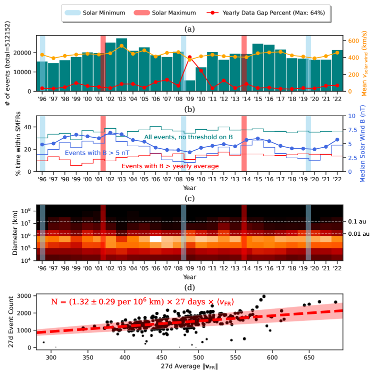
Figure 11: (a) Displays the number of events in each year displayed as a bar plot. Overplotted in (a) are the relative variations of the yearly averaged solar wind velocity as measured by SWE (including the entire year, not just SMFR intervals). Additionally, the solar maxima and minima are labeled. This plot demonstrates that without a threshold fixed to a particular value, the variations in SMFR count correspond to velocity variations or data gaps, not solar activity. (b) Filling factor in each year containing SMFRs (corrected for data gaps). Also included is the yearly average magnetic field strength and the filling factor with two alternative $B$ thresholds. (c) Filling factor in each year containing SMFRs within particular ranges of diameters. Brighter bins indicate a higher percentage of the year contained within SMFRs of diameters within the bin’s range of diameters. (d) Scatter plot including linear regression between each 27 day period’s average $\|\mathbf{v}_{\mathrm{FR}}\|$ and number of events. The dashed line is the fitted regression and the shaded region contains the 4$\sigma$ uncertainty. Smaller points have more data gaps. The periods with no SMFRs are not included in the scatter plot.

Figure 11 (a) shows the number of events detected from each year of data. The number is not constant, but it doesn’t exactly correspond to solar activity, either. The points in time corresponding to solar maxima and minima are displayed as red and blue vertical bars. The peak SMFR number is not exactly at solar maximum and the minimum SMFR number is not exactly at solar minimum. This implies that the SMFR counts are not directly related to solar activity, but they are related to the solar cycle. They appear to peak in the declining phase of the solar cycle. In fact, it is well known that the solar wind speed peaks during the declining phase of the solar cycle. This motivates the inclusion of the variation of the yearly average solar wind speed in Figure 11 (a), showing that the number of SMFRs is directly proportional to the average speed. The only significant deviations are during years that have major data gaps (also included in Figure 11 (a)). Figure 11 (d) confirms that the same trend applies on a timescale of 27 days (about a synodic solar rotation). This implies that the filling factor of the SMFRs is nearly constant over time. If the filling factor is constant and the velocity doubles, the number of SMFRs should double. Mathematically:

$$\derivative{N}{t}=\derivative{N}{x}\derivative{x}{t}=\derivative{N}{x}v\approx\mathrm{constant}\times v\implies\derivative{N}{x}\approx\mathrm{constant}$$

A quantitative estimate is provided by fitting the number of events to the average velocity in a given 27 day period in Figure 11 (d), yielding an estimate of ${\sim}1$ SMFR per $10^{6}$ km.

If the radial density is constant, then the filling factor containing SMFRs should also be constant. Figure 11 (b) shows the yearly integrated duration of all of the SMFRs in a given year divided by one year. In other words, it shows the percentage of a year contained within the events. From this figure, it is apparent that the temporal variation is minimal. and clearly has no correlation to the sunspot number. The variation imposed by the change of yearly average bulk solar wind speed in Figure 11 (a) is also eliminated in Figure 11 (b). It appears that approximately 35% of the solar wind contains SMFRs for the entire solar cycle. This may even be an underestimate, due to the fact that the smallest scales are not resolved (Section 5) and because some of the assumptions required in the detection process may not apply to all SMFRs. In contrast, applying the fixed 5 nT threshold results in a strong solar cycle dependence, with the filling factor dropping severely when the yearly average B drops below 5. Yet using the yearly average B instead of 5 nT gives virtually the same filling factor trend as using no threshold at all, except that the value is halved. This shows that the solar cycle dependence for the majority population is artificially imposed by the fixed 5 nT threshold.

Figure 11 (c) shows the dependence on size by plotting the filling factor (percentage of time) contained in SMFRs within a given year and range of sizes. From here it becomes apparent that despite the probability density of smaller SMFRs increasing below the smallest resolved size, the filling factor occupied by these extremely small SMFRs is very low. Most of the time is occupied by SMFRs of size between $10^{5}$ and $10^{6}$ km. These do not exhibit any sort of clear solar activity dependence. In fact there is a weak anticorrelation with solar activity, where the filling factor occupied by SMFRs around $10^{6}$ km seems to peak at solar minimum. However, looking closely at the top portion of Figure 11 (c), events of diameter above ${\sim}$0.01\text{\,}\mathrm{a}\mathrm{u}$$ appear to be significantly more common during solar maximum and have a strong correlation with solar activity. Considering CMEs tend to be on the order of 0.1 au, these would still be considered SMFRs. Due to the solar activity dependence and large size, this subpopulation is much more likely to have a solar origin.

5.3 Do SMFRs Cluster Around the Heliospheric Current Sheet?

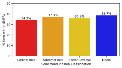
Figure 12: Filling factor for each category within SMFRs (corrected for data gaps).

Figure 12 shows the filling factor for each solar wind classification (based on Xu & Borovsky (2015)). In both of the slow solar wind categories, about 43% of the time is filled with SMFRs. The slight drop in percentage for coronal hole origin plasma might be a result of the higher speed resulting in less events fitting in the sliding windows compounded with the known fact that SMFRs tend to be slightly smaller in faster solar wind (Borovsky, 2008; Hu et al., 2018). That the filling factor is independent of solar wind type is very surprising, because Cartwright & Moldwin (2010) found that SMFRs cluster around the heliospheric current sheet (HCS), and this conclusion was in agreement with the analysis of Hu et al. (2018). If that were the case, we should have seen the highest density of SMFRs at sector reversal regions. In this subsection, we demonstrate that the apparent tendency of SMFRs to cluster around the HCS is artificial.

In their Section 7, Hu et al. (2018) analyzed the distribution of the number of days between the detected SMFRs and the nearest HCS crossing in order to compare to a similar analysis by Cartwright & Moldwin (2010). It was found that the distribution is peaked at 1 day after the nearest HCS crossing and that the SMFRs tend to cluster around the HCS boundaries. However, we point out here that looking solely at the distribution of days between SMFR times and the nearest HCS crossing is prone to statistical bias. Most of the measurements are close to the HCS, so the distribution for SMFRs must be compared to the distribution of the measurements. The distribution of the SMFR distance to the HCS is only meaningful by itself if the distance of the measurements from the HCS are uniformly distributed.

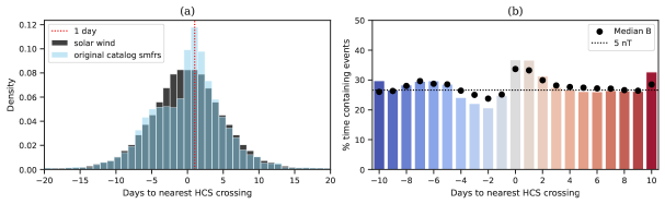
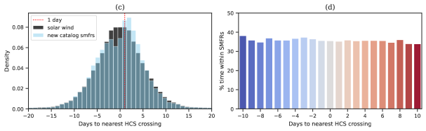
Figure 13: (a) Histogram of distance from nearest HCS crossing for original catalog’s events and for uniformly spaced timestamps. The black bars represent the distribution of distance from the HCS to points evenly spaced in time for the time interval of the original catalog. The blue bars represent the distribution of the distance from the HCS for the SMFRs in their catalog. The dotted red line demonstrates that the SMFR distribution peaks at 1 day from the HCS. (c) and (d): Same as (a) and (b) but using the data for the new list of events. Additionally, (d) is corrected for data gaps but not (b) because the data gaps are less significant in the original catalog dataset and because it used a different instrument.

In order to determine whether SMFRs are more common closer to the HCS crossings, we calculated the distances to the nearest HCS crossing for the measurements used for detection in addition to the distances for the detected SMFRs. Like Hu et al. (2018), we use L. Svalgaard’s list of HCS crossings. In Figure 13 (a), we compare their HCS distance distribution to the SMFR HCS distance distribution. From this figure, it appears that the filling factor of SMFRs is constant far from HCS crossings, reduced shortly before, and elevated shortly after. However, the changes are strongly correlated with changes in the average $B$ as a function of distance from the HCS crossing as shown in the figure, suggesting the possibility of further statistical bias.

In Figure 13 (b), we plotted the total duration of the SMFRs that are a given number of days from the nearest HCS crossing by the total time that Wind is that distance from the nearest HCS crossing (filling factor). For most of the distances, it is essentially a constant 25% with minimal variation, so there is not a strong tendency to be close to the HCS crossings. However, there is a slight decrease to around 20% right before the HCS crossing, followed by an increase to around 35% after the HCS crossing. As observed by Hu et al. (2018), the SMFRs are more likely to occur approximately one day after the HCS than during or before the HCS crossings. Figure 13 (b) also confirms the dip in the proportion of SMFRs right before an HCS crossing. The break point from a uniform distribution is within 6 days, which is close to the typical distance between HCS crossings during quiet times (considering a 4-sector HCS over the 27 day solar rotation).

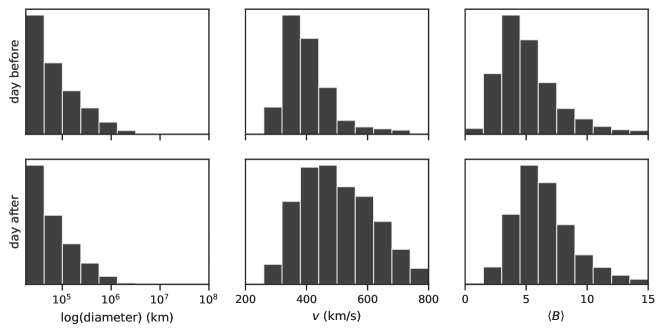
Figure 14: Comparison SMFR diameter, speed ($\|\mathbf{v}_{\mathrm{FR}}\|$), and magnetic field strength $B$ distributions before and after HCS crossings. The diameter histograms is only shown for the fully resolved range, and the other histograms are limited to typical ranges. The y axis is the proportion of samples in each bin with the y limit set to 50%. The y labels are not shown because the focus is the difference in shape of the distribution between one day before and one day after the nearest HCS crossing. Note in particular that the diameter histograms are approximately the same whereas the velocity histogram for one day after has a significantly higher proportion for higher velocities than one day before, and that the magnetic field strength has a significantly higher proportion above $5\text{\,}\mathrm{nT}$ a day after than a day before.

Figure 13 (c) is of the same format as Figure 13 (a), but using the new catalog. It is qualitatively the same, although quantitatively, the deviations of the SMFR distribution from the measurement distribution are less pronounced. However, the filling factor based on the new catalog (Figure 13 (d)) exhibits a different result from the original catalog: the filling factor is essentially the same for all distances! The disagreement with the original catalog can be explained by the magnetic field strength distributions in Figure 14. Before the HCS crossing, the average magnetic field strength is below $5\text{\,}\mathrm{nT}$. After the HCS crossing, it is above $5\text{\,}\mathrm{nT}$. Due to the fixed threshold of $5\text{\,}\mathrm{nT}$, this resulted in more events being detected after HCS crossings and less before HCS crossings in the original catalog.

If the filling factor of SMFRs does not depend on distance from HCS, why is there a difference in the number of SMFRs before and after the HCS crossing? The answer lies in Figure 14, which shows that while the size distribution of SMFRs does not differ much before or after HCS crossings, the velocity and magnetic field strength distributions are higher after the HCS crossing. This is because corotating interaction regions (CIRs), interfaces between the fast and slow solar wind, are known to “catch up” to the HCS very often (Borrini et al., 1981; Crooker et al., 1999; Huang et al., 2016; Potapov, 2018; Liou & Wu, 2021). Faster solar wind streams have higher magnetic field strength and velocity. A tendency for the number of SMFRs to increase a day after HCS crossings due to the increase in velocity. For example, if the velocity were two times higher, we would expect double the number of SMFRs if the same filling factor is the same. The small increase in filling factor in Figure 13 (d) right before the HCS crossing may be due to the fixed minimum sliding window length: A slightly higher proportion of the total duration will be filled with events when the velocity is lower, since more events can fill the sliding windows due to having a longer duration.

In summary, the radial density and filling factor of SMFRs is independent of distance from the HCS. All of the observations indicating otherwise can be understood as follows: The velocity would be expected to increase after crossing the HCS and passing the CIR, usually after less than a day (Liou & Wu, 2021). This explains the peak of the distribution a day after the HCS crossing rather than zero days, as pointed out by Hu et al. (2018) and confirmed in the above analysis. The higher velocity after the HCS results in more SMFRs being detected without affecting the filling factor. The reason the events in the original catalog have a difference in filling factor before and after the HCS, not just the number of events, is because of the $\expectationvalue{B}>$5\text{\,}\mathrm{nT}$$ threshold: $B$ increases from below to above the threshold after entering faster solar wind with stronger $B$. In short, although more SMFRs are observed when the solar wind moves faster, the filling factor of SMFRs is independent of distance from the HCS (as well as solar activity). It is constantly approximately 35%. Since the size distribution varies only slightly by distance from HCS or plasma type, this means that radial density is independent of distance from the HCS, too.

6 Physical Properties

6.1 Axial Orientation

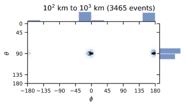
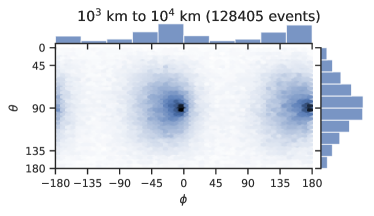
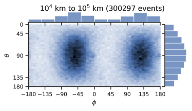
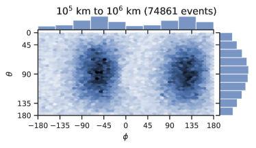
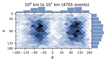
Figure 15: Joint distribution of $\hat{\mathbf{z}}$ azimuth $\phi$ (counterclockwise angle from the radial direction away from the Sun) and polar angle $\theta$ (angle from the normal direction in the RTN coordinate system) for various ranges of diameter. In the 2D histograms, darker values mean higher filling factors. The 2D histograms are generated with hexagonal binning to clearly show the shape. Furthermore, the vertical binning is by $\cos(\theta)$ instead of $\theta$ (hence the uneven spacing) because randomly oriented unit vectors naturally tend to values of $\theta$ closer to $90\text{\,}\mathrm{\SIUnitSymbolDegree}$ (by a factor of $\sin(\theta)$) but have uniformly distributed $\cos(\theta)$. The sides show the histograms of $\phi$ (on top) and $\theta$ (on the right).

Figure 15 illustrates the distribution of the axial orientation in the radial-tangential-normal (RTN) coordinate system converted to spherical coordinates. In terms of the components of $\hat{\mathbf{z}}$ in RTN coordinates, $\phi\equiv\mathrm{arctan2}(z_{T},z_{R})$ is the azimuth angle and $\theta\equiv\arccos(z_{N})$ is the polar angle. $\phi=0$ means radially outward from the Sun, and $\theta=0$ means in the normal direction (which is approximately northward), while $\theta=$90\text{\,}\mathrm{\SIUnitSymbolDegree}$$ means in the RT plane. Parker spiral alignment would have $\theta=$90\text{\,}\mathrm{\SIUnitSymbolDegree}$$ and $\phi\approx-$45\text{\,}\mathrm{\SIUnitSymbolDegree}$$ when the IMF has positive polarity (away from the Sun) and $\phi\approx$135\text{\,}\mathrm{\SIUnitSymbolDegree}$$ when it has negative polarity (towards the Sun). In Figure 15, this appears to be the case for all of the well-resolved scale ranges. Deviations from Parker spiral alignment follow a 2D Gaussian distribution, implying that they are due to random and independent processes (such as errors in determining the orientation or, alternatively, 3D effects such as the tangling of flux tubes into spaghetti as illustrated in Borovsky (2008)).

In Figure 15, there are peaks in the smallest two ranges that are shifted about $5\text{\,}\mathrm{\SIUnitSymbolDegree}$ clockwise from the (anti)radial direction. Due to the Earth’s counterclockwise orbit, the solar wind velocity relative to a spacecraft orbiting along with the Earth has a slight clockwise shift. The sign of the direction depends on the IMF polarity, not the direction of the velocity. Thus, the peaks are velocity aligned orientations. Because the temporal scale distribution continues to increase at our smallest sliding window size of 30s, it is likely that a significant number of SMFRs exist at scales below the lowest well-resolved scale in our event list (approximately $10^{4}$ km or so). It takes longer for the spacecraft through a flux rope of a given size the smaller the angle between its orientation and velocity. Thus, the many events with diameters below the resolved range would only be detected if their orientation is sufficiently close to the velocity that their duration reaches 30s. Indeed, the peaks virtually disappear when events of diameter lower than $10^{4}$ km are ignored, which is approximately the cutoff (Section 5). This explains the additional peaks close to the velocity direction.

The results in this section demonstrate that the SMFRs at all scales where the orientation distribution can be resolved have a clear tendency to follow the Parker spiral direction. This is in agreement with the results of the original catalog, providing further validation for the extended range of sizes.

6.2 Field-Aligned Flows in SMFRs

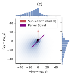
Figure 16: (a) Histogram of Wal$\acute{\text{e}}$n slope. The black bars include all events, while the blue and red respectively represent events with extremely strong and not so strong correlation between $\mathbf{v}-\mathbf{v}_{\mathrm{HT}}$ and $\mathbf{v}_{A}$. A positive (negative) Wal$\acute{\text{e}}$n slope indicates a flow (anti)parallel to the magnetic field. (b) Histogram of correlation between $\mathbf{v}-\mathbf{v}_{\mathrm{FR}}$ and $\mathbf{v}_{A}$. (c) Histogram of velocity difference between $\expectationvalue{\mathbf{v}}$ and $\mathbf{v}_{\mathrm{FR}}$. The plot indicates a tendency for the velocity fluctuations to be sunward along the Parker spiral in the flux rope frame of reference.

The Wal$\acute{\text{e}}$n slope distribution, measuring Alfv$\acute{\text{e}}$nicity, is plotted in Figure 16 (a). In Figure 16 (b), the distribution of the correlation is shown as well. When the correlation is low, the Wal$\acute{\text{e}}$n slope tends to be estimated as 0 since a clear linear relationship cannot be found. For the most part, the results are consistent with the results we obtained by reanalyzing the original catalog (Figure 3). Most of the SMFRs have non-negligible field-aligned velocity fluctuations that are comparable to but less than the Alfv$\acute{\text{e}}$n velocity. Both along and opposite to the magnetic field direction, the absolute value appears to be normally distributed. An additional population centered around 0 is present but can be explained as a consequence of measurement uncertainties resulting in low correlation for events with weak field-aligned flows resulting in a Wal$\acute{\text{e}}$n slope tending to zero. However, unlike the center in Figure 3, the center of the normal distributions in Figure 16 (a) appears to be lower than 0.7. This is most likely because the lack of the 5 nT threshold enables more flux ropes to be detected that are not in coronal hole origin solar wind streams, hence less Alfv$\acute{\text{e}}$nic and lower $B$. This also explains the difference between our result and the result of Borovsky (2020a), since their statistics are based only on Alfv$\acute{\text{e}}$nic events.

If the velocity fluctuations in our detected events do not average to zero, does that mean that they are actually waves, not propagating structures? Waves can be broadly defined as structures that propagate relative to the so-called background bulk fluid velocity, whatever that is. There is a difference between the flux rope velocity and the average bulk fluid velocity within the flux rope. Figure 16 (c) demonstrates that the majority of SMFRs move faster than the average of the velocity within the SMFRs by a finite but sub-Alfv$\acute{\text{e}}$nic amount, usually less than half the Alfv$\acute{\text{e}}$n speed. Thus from the perspective of the particles within a flux rope structure, most flux ropes propagate away from the Sun along the Parker spiral. In the flux rope frame of reference, the plasma tends to flow sunwards along the Parker spiral.

The velocity fluctuations, being field aligned, will have a mean fluctuation that is aligned with the flux rope axis. Since the velocity fluctuations have a preferred direction, the rest from of the solar wind plasma is not necessarily the average velocity $\expectationvalue{\mathbf{v}}$. Previous studies suggest that the solar wind frame of reference is in fact $\mathbf{v}_{\mathrm{HT}}$, the velocity of the advected structures (e.g. Němeček et al. (2020)). The variations in both magnetic field and plasma velocity, as well as variations in properties related to the magnetic structure like density, specific entropy, plasma beta, helium abundance, and electron heat flux are all advected with velocity $\mathbf{v}_{\mathrm{HT}}$ (Borovsky, 2020a). This suggests that the rest frame is in fact $\mathbf{v}_{\mathrm{HT}}$ ($\equiv\mathbf{v}_{\mathrm{FR}}$), not $\expectationvalue{\mathbf{v}}$. With this information in mind, it is more likely that we are dealing with advected structures, not waves.

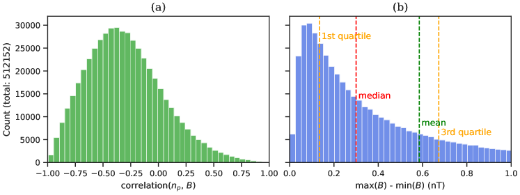
Figure 17: (a) Histogram of correlation between proton number density and magnetic field strength. (b) Histogram of the maximum B minus minimum B in the closed part of the reconstructed cross section. Demonstrates that unlike pure Alfv$\acute{\text{e}}$n waves, SMFRs have anticorrelated $n_{p}$ and $B$ as well as a nonzero, measurable change in $B$.

Advected structures are often distinguished from waves by anticorrelated proton density $n_{p}$ and magnetic field strength $B$, which is not a signature exhibited by Alfv$\acute{\text{e}}$n waves. Burlaga & Turner (1976) (cited by Cartwright & Moldwin (2010) to justify the exclusion of Alfv$\acute{\text{e}}$nic fluctuations from SMFR detection) pointed out ‘Alfv$\acute{\text{e}}$n waves’ from spacecraft observations have nonzero, measurable fluctuation in $B$, which cannot be incompressible Alfv$\acute{\text{e}}$n waves but can be compressible Alfv$\acute{\text{e}}$n waves. (Burlaga & Ogilvie, 1970) found weakly anticorrelation between total thermal pressure and magnetic pressure on a timescale of ${\sim}$1 hour, evidence for the existence of pressure-balanced nonpropagating structures. Denskat & Burlaga (1977) found evidence that some Alfv$\acute{\text{e}}$nic fluctuations may contain tangential discontinuities and other types of static structures, suggesting they are probably not pure Alfv$\acute{\text{e}}$n waves. Anticorrelation between $n_{p}$ and $B$ have been used by previous studies as evidence of the existence of pressure balanced structures to the exclusion of Alfv$\acute{\text{e}}$n waves (e.g. Vellante & Lazarus (1987); Matthaeus et al. (1990)). Figure 17 (a) shows a strong tendency for negative correlation between $n_{p}$ and $B$. This suggests that the detected SMFRs correspond to the long-observed pressure balanced structures, not Alfv$\acute{\text{e}}$n waves. A property expected for incompressible Alfv$\acute{\text{e}}$n waves is a constant magnetic field strength $B$, but Figure 17 (b) demonstrates that for the detected events, the range of magnetic field strength values is usually significantly higher than the measurement uncertainty (which is less than 0.1 nT; not shown here, the histogram of the logarithm shows that the range of magnetic field strength is log normally distributed). Since $|R_{w}|$ is usually significantly less than 1, even pure compressible Alfv$\acute{\text{e}}$n waves cannot satisfactorily explain the data. Considering also that the Alfv$\acute{\text{e}}$nic events have most of the same statistical properties as the non-Alfv$\acute{\text{e}}$nic events, it is difficult to consider the Alfv$\acute{\text{e}}$nic events to be pure Alfv$\acute{\text{e}}$n waves and not flux ropes.

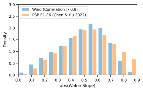
Figure 18: Comparison of absolute value of Wal$\acute{\text{e}}$n slope with the distribution derived from PSP’s first six encounters by Chen & Hu (2022). Only the absolute value is shown because most of those PSP encounters were during periods of antiradial magnetic field, so the Wal$\acute{\text{e}}$n slope from the PSP observations was preferentially positive. For the Wind data, only samples with at least 0.8 correlation are included in the histogram, so that the criteria is the same as the one used by Chen & Hu (2022). Additionally, since we require that the Wal$\acute{\text{e}}$n slope is less than 0.9, we do not include bins above 0.9. This figure shows that the peak of the distribution is the same. The differences in the other parts of the distribution may be due to the differences in plasma types observed by the two spacecraft.

Considering that the previous understanding is that SMFRs near the Sun are more Alfv$\acute{\text{e}}$nic than SMFRs away from the Sun, it is pertinent to compare our results to recent findings from PSP. Figure 18 compares our derived Wal$\acute{\text{e}}$n slope distribution to the one derived by (Chen & Hu, 2022) from PSP’s first 6 encounters. The most outstanding feature of this figure is that the peak is the essentially same at 1 au and at PSP. However, there are some significant differences away from the peak. It is unclear whether this difference is due to the radial difference or the difference in plasma types observed by the two spacecraft. If PSP happened to observe more Alfv$\acute{\text{e}}$nic solar wind than non-Alfv$\acute{\text{e}}$nic solar wind, for example, then such a difference between PSP and 1 au observations should occur even without any radial evolution of the Alfv$\acute{\text{e}}$nicity. Since the peak of the distribution is the same, it seems that there is minimal variation of the Wal$\acute{\text{e}}$n slope between the inner heliosphere and 1 au, if any. Although it is well-known that the “Alfv$\acute{\text{e}}$nicity” in the sense of cross helicity decreases away from the Sun, this does not necessarily mean that the “Alfv$\acute{\text{e}}$nicity” in terms of Wal$\acute{\text{e}}$n slope has any radial dependence: the Alfv$\acute{\text{e}}$n speed decreases away from the Sun, which reduces the energy of Alfv$\acute{\text{e}}$nic fluctuations. Since cross helicity is related to the energy of the Alfv$\acute{\text{e}}$nic fluctuations, this would reduce the cross helicity while leaving the Wal$\acute{\text{e}}$n slope the same.

6.3 Magnetic Flux, Twist, and Current Density

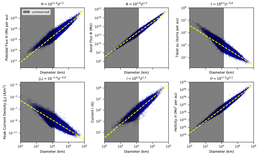
Figure 19: Scatter plots of $\Psi$, $\Phi$, $\tau$ as functions of diameter. The shaded region, with cutoff at $$600\text{\,}\mathrm{km}\text{\,}{\mathrm{s}}^{-1}$\times$30\text{\,}\mathrm{s}$$, indicates where the smallest sliding windows cannot detect SMFRs of that size for orientations too far from radial, so the reconstructions and derived parameters are less reliable in this range.

Using the reconstructed cross sections from the output of our improved detection algorithm, we have access to more quantitative information on the detected SMFRs than previous studies. Because magnetic flux is conserved under ideal MHD, it is useful to view the axial and poloidal flux in particular. We estimated the axial flux $\Phi$ by integrating $\int B_{z}dxdy$ over the closed region of the recovered cross section (Appendix B) and the poloidal flux per unit length $\Psi$ as the difference between the maximum and minimum values of $A$ in the closed region. Using these two, we estimated the average twist (number of turns turns per unit length) as $\tau=\Psi/\Phi$ (which is the equation for the twist of a cylindrical flux rope having uniform twist). Additionally, we calculated the 2.5D helicity (per unit length) as $H=\int(A-A_{0})B_{z}dxdy$ where $A_{0}$ is the the value of $A$ at the outermost field closed transverse field line and the integration is over the closed region of the flux rope (Hu et al., 1997).

Figure 19 shows how these parameters vary as a function of flux rope diameter. We only consider the range of diameters that are fully resolved in terms of axial orientation and thus have more reliable reconstructions. From here, it appears that the axial flux is directly proportional to the area, suggesting that the axial field strength is independent of the flux rope scale. However, although the poloidal flux is related to the diameter, it is not directly proportional. Instead, it is related with a power law index of 1.2. These relationships mean that the axial magnetic field strength is largely independent of the flux rope size, whereas larger flux ropes have stronger poloidal magnetic field strength on average. The power law indices appear to remain the same regardless of solar activity level or the yearly average IMF strength (not shown), although both the poloidal and axial flux distributions appear to shift proportionately to changes in average IMF strength.

We also calculated the peak axial current density $j_{z}$ from the polynomial fit to $P_{t}^{\prime}(A)$. Figure 19 shows that the peak axial current density shares the same power law as the twist and that the total current shares the same power law as the poloidal flux. The current density decreases with size, whereas the total current increases with size.

Table 2: Median value of properties in different solar wind plasma types calculated using only events in the well-resolved range of diameters.

Quantity	Coronal Hole	Streamer Belt	Sector Reversal	Ejecta
$\Phi/A$	5.07 nT	4.84 nT	3.88 nT	9.66 nT
$2\Psi/d$	0.78 nT	0.70 nT	0.58 nT	0.94 nT
$|R_{w}|$	0.60	0.46	0.29	0.47
$\|\mathbf{v}_{\mathrm{FR}}\|$	608 km/s	434 km/s	348 km/s	446 km/s
$\|\langle\mathbf{v}_{\mathrm{sw}}\rangle\|$	590 km/s	426 km/s	346 km/s	429 km/s
$\langle n_{p}\rangle$	2.8 per cc	4.6 per cc	7.40 per cc	5.2 per cc
$\langle T_{p}\rangle$	20.0 eV	9.0 eV	3.8 eV	8.9 eV

6.4 Plasma Type Dependence

Table 2 shows how certain SMFR properties depend on the plasma type. The axial and poloidal fluxes for a given size tend to be higher in faster plasma types such as coronal hole origin plasma and ejecta, but lower in slower plasma types such as streamer belt origin plasma and sector reversal regions. Conversely, this implies that larger flux ropes are more common in slower solar wind streams, consistent with previous results (Borovsky, 2008; Hu et al., 2018). The Alfv$\acute{\text{e}}$nicity of SMFRs is significantly higher in coronal hole origin plasma. Flux rope speed and plasma speed are both higher in faster solar wind types, but the average plasma speed is slightly lower in all types (even ones with low Alfv$\acute{\text{e}}$nicity) due to the sunward velocity fluctuations in the flux rope frame. This is consistent with the general understanding that the fast solar wind is more Alfv$\acute{\text{e}}$nic whereas the slow solar wind is less Alfv$\acute{\text{e}}$nic. Since the distribution is only slightly different for each non-ejecta solar wind plasma type, it is natural to assume that it is the same phenomenon that is observed in all three. It is unclear whether the difference with SMFRs in ejecta plasma is due to them being a different structure altogether or due to a difference in the plasma conditions in ejecta plasma. For example, if they all form locally through turbulence, the plasma conditions should have a significant effect on the properties of the SMFRs.

Another observation is that in Table 2, the SMFRs are less dense and hotter in faster solar wind types while being more dense and cooler in slower wind types. If one estimates a characteristic pressure by multiplying average temperature by average density, the pressure coronal hole origin plasma is higher than the streamer belt plasma by a factor of $1.36$ and which, in turn, has a pressure higher than that of sector reversal plasma by a factor of $1.48$. These properties are consistent with the well-known properties of the fast and slow solar wind. Since the faster solar wind types have higher pressure, compression is a possible reason for the slight decrease in size for a given magnetic flux in faster types compared to slower types.

7 Discussion and Conclusions

In summary, we have developed an improved version of the GS-based automated detection algorithm, demonstrated its improved speed and reliability qualitatively and quantitatively with simulated data, and applied it to 27 years of Wind data. The improved performance enabled extending the detection to a larger range of sizes with significantly less computational resources. The improved reliability justified the removal of the $B>$5\text{\,}\mathrm{nT}$$ threshold, motivated by previous findings that properties of SMFRs such as $B$ correspond to the surrounding solar wind. This revealed the statistical bias underlying previous conclusions regarding solar activity and distance to HCS dependence. We summarize the findings as follows.

1. SMFR diameter is log-normally distributed. The parameters of the log-normal distribution depend on solar wind type. Among non-ejecta solar wind types, the distribution extends to larger values in slower types, consistent with previous findings (Borovsky, 2008; Hu et al., 2018). We have shown that this may be a consequence of compression (Table 2), although it could alternatively be related to proximity to the HCS. In ejecta plasma, the distribution is also log-normal but despite the relatively fast speed, its size range extends further than other types.

2. The apparent solar activity dependence of the SMFR count was eliminated by removing the $B$ threshold or by using the yearly average as a flexible threshold instead. The remaining variation of SMFR count per year is consistent with proportionality to the average yearly velocity. This proportionality was also verified to hold at a timescale of a synodic solar rotation. The slope of the proportionality yielded an estimated radial density of ${\sim}1$ SMFR per $10^{6}$ km.

3. The filling factor, or percentage of measurements within SMFRs, is independent of solar activity without a fixed $B$ threshold (having a constant value of approximately 35%). With the fixed 5 nT threshold, there is a strong correlation between the yearly average solar wind $B$ and the filling factor of the SMFRs with $B$ above the threshold. With the yearly average $B$ as a flexible threshold, the filling factor is again independent of solar activity.

4. The majority of the filling factor is contributed by SMFRs of diameters between $10^{5}$ and $10^{6}$ km. These do not exhibit a solar activity dependence. The contribution to the filling factor by the largest SMFRs, above approximately 0.01 au in diameter, do exhibit a strong solar activity dependence, suggesting that they are transient events.

5. The filling factor and radial density of SMFRs are independent of solar wind type and distance to the HCS. This is evidenced by the consistency of the linear relationship between velocity and SMFR count despite the well-known fact that the HCS is nearly vertical during solar maximum, affecting the proximity to the HCS throughout a solar rotation. Moreover, the rate at which each solar wind type observed changes changes throughout the solar cycle, so a major solar activity dependence should have been observed if SMFRs were more common in a certain solar wind type. It is also supported by the virtual independence of the filling factor on the categorization of the solar wind type by the Xu & Borovsky (2015) method (Figure 12).

6. The previous finding of HCS distance dependence reported by Cartwright & Moldwin (2010) and Hu et al. (2018) was demonstrated to be a consequence of statistical bias. The reason for the peak of the distribution of distance to the nearest HCS crossing in both studies is that the same peak is found in the distribution of the measurements’ distance to the nearest HCS crossing. We found that the reason that Hu et al. (2018) found the peak was 1 day after the HCS crossing is because of the known fact that CIRs catch up to the HCS, resulting in faster solar wind about a day after HCS crossings with $B>$5\text{\,}\mathrm{n}\mathrm{T}$$, resulting in both a higher event count (for both the new and old catalogs) and a higher filling factor (for the old catalog only, due to the 5 nT threshold).

7. The orientation of SMFRs at all scales where the orientation can be resolved, including the largest scales, is consistent with Parker spiral alignment (Figure 15). This is consistent with previous studies (Borovsky, 2008; Hu et al., 2018) but is demonstrated in this study across a wider range of scales.

8. Most SMFRs at 1 au have significant Alfv$\acute{\text{e}}$nicity (field-aligned flows) as determined by the Wal$\acute{\text{e}}$n slope. Although Gosling et al. (2010) found that early SMFR lists did not contain many Alfv$\acute{\text{e}}$nic events, Alfv$\acute{\text{e}}$nic events were generally excluded by previous studies. The reason that previous applications of GS detection did not report a significant number of Alfv$\acute{\text{e}}$nic SMFRs was that the use of the average velocity as the reference frame led to a Wal$\acute{\text{e}}$n slope biased to 0. Applications to PSP (Chen et al., 2020, 2021; Chen & Hu, 2022) used the HT frame, which led to the correct Wal$\acute{\text{e}}$n slope. Corrected calculation applied to the original catalog’s events reveals that most of the events in the original catalog have high Alfv$\acute{\text{e}}$nicity, which we also validated using a reference frame-independent method (Chao et al., 2014).

9. Despite the high Alfv$\acute{\text{e}}$nicity, Alfv$\acute{\text{e}}$nic SMFRs exhibit signatures inconsistent with pure Alfv$\acute{\text{e}}$n waves. These include the nonzero change in $B$ (incompatible with small-amplitude Alfv$\acute{\text{e}}$n waves) and the anticorrelation between magnetic field strength and density (whereas Alfv$\acute{\text{e}}$n waves should have a positive correlation (Vellante & Lazarus, 1987)). Additionally, the statistical properties of Alfv$\acute{\text{e}}$nic SMFRs are consistent with those of non-Alfv$\acute{\text{e}}$nic SMFRs, suggesting that they are the same phenomenon.

10. Comparison of the Alfv$\acute{\text{e}}$nicity distribution at 1 au (our event list) and PSP (Chen & Hu, 2022) results in little difference between the two distributions (Figure 18). The peak of the distribution is the same. The PSP results have slightly less low-Alfv$\acute{\text{e}}$nicity events and slightly more high-Alfv$\acute{\text{e}}$nicity events. It is unclear if these disagreements are due to differences in methodology, radial evolution, or PSP spending more time in Alfv$\acute{\text{e}}$nic soolar wind.

11. Using the additional information provided by the new detection method, we found that poloidal flux $\Psi$, axial flux $\Phi$, twist $\tau$, current density $j_{z}$, and helicity $H$ follow power laws with respect to diameter. The axial flux power law of $\Phi\propto d^{2.0}$ implies that the average axial field strength $\expectationvalue{B_{z}}\propto\Phi/d^{2}$ is independent of size. The poloidal flux power law $\Psi\propto d^{1.2}$ implies that the average poloidal field strength $\expectationvalue{B_{\phi}}\propto\Psi/(2d)$ is not independent of size, but increases slightly with size as $\expectationvalue{B_{\phi}}\propto d^{0.2}$. As a consequence, larger SMFRs have slightly higher total field strength. The helicity power law $H\propto d^{3.2}$ suggests that if the larger SMFRs form by merging of smaller SMFRs, either helicity or total area is not conserved (if both were conserved, we would have $H\propto d^{2.0}$). Presumably, area is less likely to be conserved. These power laws can be compared to large-scale MHD simulations in future studies.

12. By comparing the average properties of SMFRs in different solar wind types, we confirmed that the SMFR properties closely follow the properties of the surrounding solar wind. For example, magnetic field strength and temperature are highest in coronal hole-origin plasma, whereas density is highest in sector reversal region plasma. Similarly, Alfv$\acute{\text{e}}$nicity is higher in coronal hole-origin plasma.

SMFRs were originally seen as transient structures, but results from this and other recent studies (Section 1) suggest that the solar wind is a sea of SMFRs. The primary candidates for the origin of SMFRs according to the earliest studies were relatively small CMEs (Feng et al., 2008) or reconnection across the HCS (Moldwin et al., 1995, 2000; Cartwright & Moldwin, 2010). However, for most SMFRs, the lack of solar activity dependence of the radial density makes it unlikely that they are related to small CMEs. The complete independence of distance from the HCS suggests that it is unlikely that reconnection across the HCS is a major source of SMFRs, either. Of course, it is likely that both of these mechanisms contribute sub-populations, since some solar eruptions have been directly linked to SMFRs at 1 au (Rouillard et al., 2011). These SMFRs would be transients as opposed to filling the solar wind. However, if one is to study them, it is not sufficient to simply look for long events or events with elevated $B$, as most of those may just be particularly large fluctuations, the tails of the log-normal distributions of the main population SMFRs’ size and magnetic field strength. Additional factors such as having significantly different physical properties from surrounding solar wind should be considered. In fact, since SMFRs above ${\sim}0.01$ au do appear to have a strong solar cycle dependence (Figure 11 (c)), this may be possible to use as a threshold to identify transient SMFRs. However, unlike ICMEs, these large SMFRs are aligned with the Parker spiral, just like smaller SMFRs (Figure 15).

Within the sea of flux ropes model, the origin and dynamics of the flux ropes remain contested. Borovsky (2008) suggests that solar wind flux tubes typically do not interact through reconnection due to the expansion of the solar wind. However, others believe that reconnection processes result in constant destruction, creation, and merging. Greco et al. (2009) and many others have demonstrated how MHD turbulence can generate flux ropes with waiting times similar to those observed in situ between current sheets. This is often cited as evidence of local generation of the current sheets via turbulence, but it can result from repeated reconnections causing random multiplications of structure sizes (Matthaeus & Goldstein, 1986), and this process can alternatively happen at the Sun. The non-Gaussian current density distribution observed by Greco et al. (2009) was found to be similar to the in-situ SMFRs by Zheng & Hu (2018), which may be evidence of local generation via turbulence, but it is in fact not independent evidence from the log-normal distribution of size, since current density is related to size by a power law. As of now, it is unclear whether the structures are generated locally or originate as structures from the Sun (in which case, it is unclear to what extent they evolve through reconnection processes between the Sun and 1 au).

We have shown that using the correct calculation of the Wal$\acute{\text{e}}$n slope, the Alfv$\acute{\text{e}}$nicity of SMFRs tends to be high even at 1 au. The similarity of the Wal$\acute{\text{e}}$n slope distribution between the PSP results and the 1 au results (Figure 18) is interesting and requires further research. However, they usually contain what appear to be embedded Alfv$\acute{\text{e}}$n waves. Relative to its average plasma velocity, when field aligned flows are present, the flux rope structure tends to propagate outward (antisunward) along the Parker spiral at slightly less than the Alfv$\acute{\text{e}}$n speed; equivalently, in the flux rope frame of reference, there is a sub-Alfv$\acute{\text{e}}$nic sunward plasma flow. The result of antisunward propagation was found based on HT analysis in previous studies of SMFRs observed by PSP (Chen & Hu, 2022) and of general Alfv$\acute{\text{e}}$nic magnetic structure in the solar wind (Borovsky, 2020a). Paschmann et al. (2013) also found that directional discontinuities, both rotational and tangential, propagate antisunward based on electron strahl measurements combined with HT analysis. Considering the abundance of SMFRs, it is likely that most directional discontinuities are related to SMFRs. Similarly, while fluctuations in the solar wind are commonly attributed to outward-propagating Alfv$\acute{\text{e}}$n waves (Belcher & Davis, 1971), SMFRs appear to be uniformly present in all solar wind types, Alfv$\acute{\text{e}}$nic or not. Thus, a significant portion of, if not the majority of, the Alfv$\acute{\text{e}}$n waves at 1 au appear to be embedded within SMFRs.

What causes the embedded Alfv$\acute{\text{e}}$nic flows in SMFRs? Borovsky (2020b) mentioned that perturbations perpendicular to a flux tube’s axis propagate along the axis relative to the plasma at a speed related to the Alfv$\acute{\text{e}}$n speed (see references therein). Such a propagating disturbance is essentially a torsional Alfv$\acute{\text{e}}$n wave. Within the model of fossil structures connected to the Sun, they suggested that the perturbations could be due to the shuffling of flux tubes at the Sun. This is a plausible explanation for the common field-aligned flows that are more or less the same at 1 au and PSP. However, field-aligned flows can also occur through local processes (see, for example, the field-aligned flows in the benchmark MHD simulation in Figure 7). Whether the perturbations originate from the Sun or throughout the solar wind, one would still expect them to mostly propagate away from the Sun because of the super-Alfv$\acute{\text{e}}$nic speed of the solar wind.

The structure of SMFRs requires the magnetic field to rotate about a central axis. These deflections could be associated with switchbacks (SBs), the study of which has become quite popular due to their prominence in PSP observations (Bale et al., 2019; Kasper et al., 2019). As for SMFRs, numerous mechanisms have been proposed to explain the generation of SBs (e.g., Squire et al. (2020); Ruffolo et al. (2020); Drake et al. (2021); Huang et al. (2023)). Some mechanisms propose a solar origin, while others propose a local origin. Due to the numerous plausible origin mechanisms, it is likely that a number of mechanisms have varied levels of contributions at different distances from the Sun. Observationally, Pecora et al. (2022) showed that the occurrence of SBs per unit length decreases sharply within 0.2 au of the Sun, whereas it increases gradually beyond 0.2 au, implying that local dynamics play an important role. Drake et al. (2021) discussed how flux ropes can appear as switchbacks in PSP observations. By including SMFRs with high Alfv$\acute{\text{e}}$nicity, Chen et al. (2021); Chen & Hu (2022) demonstrated that many SBs observed by PSP are related to SMFRs. We have found that SMFRs at 1 au have essentially the same Alfv$\acute{\text{e}}$nicity as SMFRs observed by PSP, which means that they can also appear as SBs even if Alfv$\acute{\text{e}}$nicity is required.

Interestingly, as we have found to be the case with SMFRs, SB occurrence is correlated with bulk velocity (Mozer et al., 2021; Jagarlamudi et al., 2023). We have shown that the occurrence of SMFRs is correlated with the average bulk velocity as a consequence of a constant radial density. If we find that SBs, too, have constant radial density, that would be additional observational evidence that they are rotations of the magnetic field caused by structures such as SMFRs. However, evaluating precisely whether the radial density of SBs is constant will be challenging because the types of solar wind and levels of solar activity observed by PSP are limited, and there can be noticable fluctuations in SMFR counts even on the timescale of a solar rotation (Figure 11). Nevertheless, this is an interesting work to be carried out in the future.

Future studies of SMFRs should take into consideration some of the points we have raised regarding the detection of SMFRs and the statistical interpretation of the results:

1. Variation in the number of events must be interpreted with caution. A fixed threshold on $\expectationvalue{B}$ can cause significant statistical bias because not all SMFRs are transients. In MHD simulations and observations, the SMFR $B$ rarely differs significantly from the surrounding plasma. Removing the threshold only increases the number of events by approximately a factor of two, but it completely changes the conclusions regarding solar activity dependence. The distribution of distance to large-scale structures such as the HCS needs to be compared with the overall measurements’ distribution. It may be that events appear to be close to or far from a given large-scale structure, but in fact they share the same distribution of distance to the structure as arbitrarily chosen points in time.

2. Alfv$\acute{\text{e}}$nicity, or correlation between changes in velocity and magnetic field, can be measured through the slope of the Wal$\acute{\text{e}}$n relation $\delta\mathbf{v}\equiv\mathbf{v}-\mathbf{v}_{\mathrm{HT}}\propto\mathbf{v}_{A}$. It must be evaluated in the HT frame (Khrabrov & Sonnerup, 1998), which differs from $\expectationvalue{v}$ when $\expectationvalue{\delta\mathbf{v}}\neq 0$. Averaging over a single flux rope will result in a scatter plot where all of the components are centered on the origin, resulting almost invariably in a Wal$\acute{\text{e}}$n slope of zero. Averaging over a longer interval may be less problematic, but because the Alfv$\acute{\text{e}}$nic disturbances have a preferential direction (antisunward), it may still give inaccurate results. Alternatively, the Wal$\acute{\text{e}}$n slope may be evaluated using a frame-independent method (Chao et al., 2014), which produces the same statistical results as the HT frame (Figure 3).

3. A strong field-aligned Alfv$\acute{\text{e}}$nic flow does not necessarily mean an event candidate is a pure Alfv$\acute{\text{e}}$n wave. From a theoretical point of view, Alfv$\acute{\text{e}}$nic flows are expected to be observed in flux ropes, since there are many processes that can cause them (see Gosling et al. (2010) and references therein). Other factors must be considered to distinguish pure Alfv$\acute{\text{e}}$n waves from SMFRs, such as a nonzero change in magnetic field strength or anticorrelation between magnetic field strength and density.

A major but necessary limitation of this study is that the events are detected based on a single spacecraft. A single spacecraft cannot measure the gradient of the magnetic field, so the 2D assumption that the GS method is based on cannot be directly validated. Even if the 2D assumption is correct and there are flux ropes present, if the wrong boundaries are selected, the reconstructed cross section will be totally inaccurate, as demonstrated in Section 3. Nevertheless, the usage of single-spacecraft data was necessary for the long period of time that it afforded, and our benchmarking against an MHD simulation suggests that most of the detected events are flux ropes even if the reconstruction is inaccurate, especially those with more than 30 data points (Table 1). While only single spacecraft measurements are available to use for such a large-scale statistical study as this one, missions such as MMS can be used to determine the reliability from single spacecraft detection. In a forthcoming study, we will use a novel GS-inspired technique to detect and reconstruct SMFRs from MMS data to validate the findings in this and other single spacecraft studies.

The source code for the new detection algorithm is available at https://github.com/hafarooki/PyMFR. For an easy-to-read CSV file containing basic information about each event, as well as plots for each event, see https://doi.org/10.6084/m9.figshare.24547810. For the version of the code used in this paper, together with the code for downloading and processing data, running the detection algorithm, and generating figures, along with the data used, see https://doi.org/10.6084/m9.figshare.24547798. There is much more insight to be gained from the new database in future studies. For example, why is the Wal$\acute{\text{e}}$n slope similar for flux ropes near the Sun and at 1 au, having the same peak in the distribution? Can the power law for poloidal and axial magnetic flux help to determine the origin of the SMFRs? Are all of the observed statistical properties of SMFRs compatible with results from MHD simulations? What other information can be derived from this study’s novel database containing on the order of $10^{5}$ flux rope cross sections derived from GS reconstruction? These questions should be investigated by forthcoming studies.

8 Acknowledgements

We thank the teams at NASA for providing the Wind spacecraft data used for this study. We gratefully acknowledge support from NASA grant 80NSSC20K1282 and NSF grants AGS-2229064/2229065, OAC-2320147, and OPP-2032421. J.L was supported by NSF grant, AGS 2114201. F. Pecora is supported by PSP HelioGI under grant number 80NSSC21K1765 at the University of Delaware. The simulations have been performed at the Newton cluster at University of Calabria and the work is supported by “Progetto STAR 2-PIR01 00008” (Italian Ministry of University and Research). S. Servidio acknowledges supercomputing resources and support from ICSC–Centro Nazionale di Ricerca in High Performance Computing, Big Data and Quantum Computing–and hosting entity, funded by European Union–NextGenerationEU. H. Farooki thanks Qiang Hu, Lynn B. Wilson, Nada al-Haddad, Robert T. Wicks, Ben Lynch, Bill Matthaeus, Paul Cassak, Jimmy Juno, Charles Farrugia, Kyung-Eun Choi, Kristopher Klein, Joe Borovsky, Brian Welsch, Laxman Adhikari, Sanchita Pal, No$\acute{\text{e}}$ Lugaz, Wenyuan Yu, and Phil Isenberg for helpful comments and discussions.

Appendix A Theoretical Background

A.1 The Grad-Shafranov (GS) Technique

For any 2.5D magnetic field ($\partialderivative*{z}=0$ but $B_{z}(x,y)\neq 0$), we can write the magnetic field in terms of a magnetic vector potential $\mathbf{A}$ as $\mathbf{B}=\curl{\mathbf{A}}=\partialderivative{A}{y}\hat{\mathbf{x}}-\partialderivative{A}{x}\hat{\mathbf{y}}+B_{z}(x,y)\hat{\mathbf{z}}$ where $A\equiv\mathbf{A}\dotproduct\hat{\mathbf{z}}$. The significance of $A$ can be seen by taking its gradient along the magnetic field direction: $\gradient{A}\dotproduct\mathbf{B}=\partialderivative{A}{x}\partialderivative{A}{y}-\partialderivative{A}{y}\partialderivative{A}{x}=0$. This implies that $A$ is a field line invariant (constant along transverse field lines). Thus the contours of $A$ in the plane perpendicular to $\hat{\mathbf{z}}$ (isosurfaces of $A$ when viewed in 3D) are transverse (in-plane) magnetic field lines. Using Ampere’s law, $\mu_{0}j_{z}=\hat{\mathbf{z}}\dotproduct\curl{\mathbf{B}}=\partialderivative*{B_{y}}{x}-\partialderivative*{B_{x}}{y}=-\partialderivative*[2]{A}{x}-\partialderivative*[2]{A}{y}=-\laplacian{A}$, so the source of $A$ is the axial current density:

$$\laplacian{A}=-\mu_{0}j_{z}$$ (A1)

Evaluating the flux rope velocity $\mathbf{v}_{\mathrm{FR}}$ requires finding the frame of reference in which the magnetic structure does not change, i.e. $\partialderivative*{\mathbf{B}}{t}=-\curl{\mathbf{E^{\prime}}}=0$, where $\mathbf{E^{\prime}}=\mathbf{E}+\mathbf{v}_{\mathrm{FR}}\crossproduct\mathbf{B}$. A sufficient (but not necessary) condition for this is simply that $\mathbf{E}=-\mathbf{v}_{\mathrm{FR}}\crossproduct\mathbf{B}$ and $\mathbf{E^{\prime}}=0$. Such a reference frame is called a deHoffman-Teller or HT frame, denoted $\mathbf{v}_{\mathrm{HT}}$ (De Hoffmann & Teller, 1950). An optimal HT frame can be found efficiently using a linear algebra technique (Khrabrov & Sonnerup, 1998). Typically, $\mathbf{v}_{\mathrm{HT}}$ is found assuming that the solar wind electric field is $\mathbf{E}=-\mathbf{v}\crossproduct\mathbf{B}$, since we operate at MHD scales and direct measurements of the electric field are not always available. Furthermore, the proton velocity is usually used to calculate $\mathbf{E}$, although if quality electron velocity measurements are available, they could provide more reliable results (Khrabrov & Sonnerup, 1998; Puhl-Quinn & Scudder, 2000). A valid HT frame is usually present in the solar wind, so $\mathbf{v}_{\mathrm{FR}}\equiv\mathbf{v}_{\mathrm{HT}}$. The power of the HT frame is that it provides a strong validation of the structure being time-static, since $\mathbf{E^{\prime}}=0$ is a sufficient condition for $\partialderivative*{\mathbf{B}}{t}=0$.

If we find a valid $\mathbf{v}_{\mathrm{HT}}$, we know that the structure is approximately static over time. If $\mathbf{v}(t)=\mathbf{v}_{\mathrm{HT}}$, we can assume magnetostatic equilibrium ($\mathbf{j}\crossproduct\mathbf{B}=\gradient{p}$). It follows that $j_{x}B_{y}-j_{y}B_{x}=\partialderivative*{p}{z}=0$, so $j_{x}/j_{y}=B_{x}/B_{y}$. This is equivalent to saying that $B_{z}$ is a field line invariant for magnetostatic structures, because we also have that $\mu_{0}j_{x}=\partialderivative*{B_{z}}{y}$ and $\mu_{0}j_{y}=-\partialderivative*{B_{z}}{x}$, so $\mathbf{B}\dotproduct\gradient{B_{z}}=-\mu_{0}(B_{x}j_{y}-B_{y}j_{x})$. Moreover, $p$ is a field line invariant, since $\mathbf{B}\dotproduct\gradient p=\mathbf{B}\dotproduct(\mathbf{j}\crossproduct\mathbf{B})=0$. Assuming each transverse field line has a unique value of $A$, $B_{z}=B_{z}(A)$ and $p=p(A)$. It can be shown that $j_{z}=\derivative*{A}\quantity[p+B_{z}^{2}/2\mu_{0}]$. The quantity $p+B_{z}^{2}/2\mu_{0}$ is commonly called the transverse pressure, denoted $P_{t}$. If $\hat{\mathbf{z}}$ is known, $P_{t}(A)$ can be fitted from spacecraft measurements with an appropriate function, and the derivative can be used as $j_{z}$ and the source term for $A$. The structure in the magnetically connected region above and below the spacecraft path can be recovered by solving the GS equation as an initial value problem, a process known as GS reconstruction (Sonnerup et al., 2006).

The original GS equation and reconstruction assume a magnetostatic structure with no flow in the $\mathbf{v}_{\mathrm{FR}}$ frame. However, the HT frame is still present, and a plasma structure can still be in a stationary state if there are finite, field-aligned flows. Sonnerup et al. (2006) derived a GS-like equation and a reconstruction process for such a scenario, where the remaining flow can be written in terms of the Alfv$\acute{\text{e}}$n speed as $\Delta\mathbf{v}\equiv\mathbf{v}-\mathbf{v}_{\mathrm{FR}}=M_{A}(x,y)\mathbf{v}_{A}$, where $M_{A}\equiv\Delta v/v_{A}$ is the Alfv$\acute{\text{e}}$n Mach number in the frame $\mathbf{v}_{\mathrm{FR}}$ (not the spacecraft frame). In the general case, $B_{z}$ and $M_{A}$ are not field line invariants, but $(1-M_{A}^{2})B_{z}$ is. For the special case where $M_{A}\equiv M_{A}(A)$ is a field line invariant, Teh (2018) introduced a further simplified equation in terms of $A^{\prime}\equiv(1-M_{A}^{2})A$ rather than $A$. It is especially simplified if $M_{A}=\mathrm{constant}$, in which case $(1-M_{A}^{2})$ can be factored out, and the equation becomes:

$$\laplacian{A}=-\mu_{0}\frac{d}{dA}\quantity[\frac{B_{z}^{2}}{2\mu_{0}}+\frac{1}{1-M_{A}^{2}}p+\frac{M_{A}^{2}}{1-M_{A}^{2}}\frac{B^{2}}{2\mu_{0}}]=-\mu_{0}j_{z}\impliedby\mathrm{Eq~{}\ref{eq:Asource}}$$ (A2)

so that the approach is essentially the same as the original GS method except $j_{z}=\derivative*{(B_{z}^{2}/2\mu_{0}+p)}{A}$ must be replaced with $j_{z}=\derivative*{(B_{z}^{2}/2\mu_{0}+p/(1-M_{A}^{2})+\frac{M_{A}^{2}}{1-M_{A}^{2}}B^{2}/2\mu_{0})}{A}$. This special case has become very important in SMFR studies because recent studies found that closer to the Sun, there are few static SMFRs but still many with field-aligned flows. Observationally, SMFRs with field-aligned flows appear to have a constant $M_{A}$ that can be estimated as the Wal$\acute{\text{e}}$n slope $R_{w}$ (the slope of a linear fit through the origin $\mathbf{v}-\mathbf{v}_{\mathrm{HT}}=R_{w}\mathbf{v}_{A}$; it is sometimes estimated using a general linear fit, but we use the linear fit through the origin) (Chen et al., 2021; Chen & Hu, 2022). As we showed, SMFRs with field-aligned flows are dominant at 1 au, not just near the Sun.

A.2 Application to Spacecraft Measurements of Flux Ropes

The GS technique (summarized above) requires a coordinate system where $\partialderivative*{z}=0$. It is common to define a coordinate system (Figure 20) such that $\hat{\mathbf{z}}$ is the cylindrical axis, the spacecraft moves in the $\hat{\mathbf{x}}$ direction through the cross section (so that $\mathbf{v}_{FR}\dotproduct\hat{\mathbf{x}}<0$ since $\mathbf{v}_{\mathrm{FR}}$ is in the spacecraft’s frame of reference), and $\hat{\mathbf{y}}$ is the perpendicular direction in the cross section defined so $x=x(t)$ but $y=y_{0}$ (the spacecraft does not move in the y direction). To construct the coordinate system, it is sufficient to find $\hat{\mathbf{z}}$ and $\mathbf{v}_{\mathrm{FR}}$. From there, $\hat{\mathbf{x}}=-\mathrm{normalize}(\mathbf{v}_{\mathrm{FR}}-\hat{\mathbf{z}}(\mathbf{v}_{\mathrm{FR}}\dotproduct\hat{\mathbf{z}}))$ and the right-hand rule specifies $\hat{\mathbf{y}}=\hat{\mathbf{z}}\crossproduct\hat{\mathbf{x}}$.

Finding $\hat{\mathbf{z}}$ is essential but challenging. Using measurements from only a single spacecraft, the gradients of the magnetic field components are not specified, so $\partialderivative*{z}$ cannot be directly verified by any sufficient condition. For flux ropes observed by a single spacecraft, Hu & Sonnerup (2002) introduced a method to determine $\mathbf{z}$. In a (reasonably simple) flux rope structure, each transverse field line has a unique value of $A$ (and other field line invariants, such as $P_{t}$). Each field line (thus each value of $A$) is observed twice as a spacecraft passes through the flux rope, so $P_{t}=P_{t}(A)$. If a given $\mathbf{z}$ is the correct orientation, then the derived $A$ versus the derived $P_{t}$ should show minimal scatter since $P_{t}$ should be a single-valued function of $A$. Thus $\mathbf{z}$ is selected to minimize scatter between $P_{t}$ and $A$, quantified as the difference residue $R_{\mathrm{diff}}$ described in Hu & Sonnerup (2002). $R_{\mathrm{diff}}$ is essentially the root mean square difference between each value of $P_{t}$ and the corresponding value interpolated to match the same value of $A$ from the other side of the measurement interval, normalized by the range of $P_{t}$ to avoid selecting an orientation where $P_{t}=\mathrm{constant}$, which would imply zero current density. (Note that Hu & Sonnerup (2002) actually used evenly spaced $A$ values to get interpolated $P_{t}$ values from either side for calculating $R_{\mathrm{diff}}$ whereas Hu et al. (2018) compared each measured value to the corresponding value from the other side. The advantage of the latter approach is that it gives less bias to measurements that happen to have a large spacing in $A$, which is common at the flux rope boundary. We use the latter approach. Also, Hu et al. (2018) added a factor of $1/\sqrt{2}$, but we did not use it.) This approach usually leads to a well-determined flux rope orientation, although there is much uncertainty in distinguishing $\hat{\mathbf{x}}$ from $\hat{\mathbf{z}}$, especially if $B_{x}$ is symmetric (Hu & Sonnerup, 2002). Besides $R_{\mathrm{diff}}$, the validity of the polynomial fit to $P_{t}(A)$ required for GS reconstruction is validated using a similar quantity $R_{\mathrm{fit}}$ (introduced by Hu (2004)) which is equivalent to the root mean squared difference between the measured $P_{t}(t)$ and the fitted $P_{t}(A)$ normalized by the range ($\max(P_{t})-\min(P_{t})$).

In principle, evaluating $A(t)$ would require integrating $dA=(\partialderivative*{A}{t})dt+(\partialderivative*{A}{x})dx+(\partialderivative*{A}{y})dy$. However, the analysis is limited to time-static structures, so $\partialderivative*{A}{t}=0$. As the coordinate system is defined so that $\mathbf{v}_{\mathrm{FR}}$ is contained in the x-z plane, $dx=-v_{x,\mathrm{FR}}dt$ (it is assumed that the spacecraft is sitting still as the flux rope passes through) and $dy=0$. Therefore, once the coordinate system in terms of the measurement coordinate system is known, $A$ along the spacecraft path is given by:

$$A(x,y_{0})=\int_{x_{0}}^{x}-B_{y}dx=-|v_{x,\mathrm{FR}}|\int_{t_{0}}^{t}B_{y}dt$$ (A3)

Figure 20: Flux rope coordinate system. $\hat{\mathbf{z}}$ is the cylindrical direction along which $\partialderivative*{z}=0$. The perpendicular plane is divided into $\hat{\mathbf{x}}$ and $\hat{\mathbf{y}}$, defined so that the spacecraft only moves through the cross section along $\hat{\mathbf{x}}$ minus the motion along $\hat{\mathbf{z}}$. Therefore, the velocity of the flux rope in the spacecraft frame ($\mathbf{v}_{\mathrm{FR}}$; assumed constant) is contained in the xz plane. Since the spacecraft moves along $\hat{\mathbf{x}}$ within the cross section, the x component of $\mathbf{v}_{FR}$ must be negative, since $\mathbf{v}_{FR}$ is measured in the spacecraft frame of reference.

A.3 Automated Detection of Flux Ropes from Spacecraft Measurements

The main signature of a flux rope is the bipolar $B_{y}$ which crosses the origin once (corresponding to the field lines pointing up on one side of the cross section and down on the other) and $B_{z}$ increasing towards the center (under force-free conditions, this is necessary considering its relation to the current density). However, this signature is not visible in every coordinate system. It is often the case that in the spacecraft measurement coordinate system there is no bipolar component of the magnetic field. As a result, a simple visual inspection of timeseries measurements will miss most of the flux ropes.

Hu et al. (2018) developed an automated detection algorithm and applied it to build a catalog of SMFRs from 21 years (1996-2016) of Wind data. Their algorithm applies a sliding window to the spacecraft measurements and tests the hypothesis that a given interval is a flux rope. Thus, their algorithm is an exhaustive search algorithm. After finding the windows that are acceptable flux rope candidates, the overlapping candidates are cleaned, and the gaps between the detected events are filled with events detected using smaller sliding windows. They used sliding windows that ranged from about 6 hours to 10 minutes. For each interval, the algorithm searches the entire $4\pi$ space with coarsely separated axial orientations ($20\text{\,}\mathrm{\SIUnitSymbolDegree}$ azimuthal, $10\text{\,}\mathrm{\SIUnitSymbolDegree}$ latitudinal) for the $\hat{\mathbf{z}}$ that minimizes $R_{\mathrm{diff}}$. The algorithm determines $\mathbf{v}_{\mathrm{FR}}$ and uses the test $\hat{\mathbf{z}}$ to set up the flux rope coordinate system. Using the $\hat{\mathbf{y}}$ given by the test $\hat{\mathbf{z}}$ and $\mathbf{v}_{\mathrm{FR}}$, $A$ is calculated using Equation A3.

The original detection algorithm considers every possible interval with the $\hat{\mathbf{z}}$ that minimizes $R_{\mathrm{diff}}$. To be considered a flux rope, a given interval with its optimal $\hat{\mathbf{z}}$ must have (1) a derived $A(x,y_{0})$ with a single stationary point (a necessary condition for each transverse field line being crossed twice) that can be trimmed to the boundaries ($A_{f}=A_{0}$) without shortening the interval to the next sliding window length (with 5-minute spacing); (2) $R_{\mathrm{fit}}<0.14$ and $R_{\mathrm{diff}}/\sqrt{2}<0.12$ (with $R_{\mathrm{diff}}$ being scaled down by a factor of $1/\sqrt{2}$ to make it comparable to $R_{\mathrm{fit}}$); (3) no strong plasma flow in the $\mathbf{v}_{\mathrm{FR}}$ frame ($R_{w}<0.3$); (4) the peak $A$ corresponds to the peak $P_{t}$ ($P_{t}$ at the peak must be in the top 15%); and (5) a relatively high average magnetic field strength $\langle B\rangle>$5\text{\,}\mathrm{nT}$$ to exclude small fluctuations.

Thus, in summary, the algorithm generates a list of nonoverlapping intervals containing time-static magnetic fields satisfying the hypothesis of being 2.5D magnetostatic structures where each field line is crossed twice and having a strong axial current density and magnetic field strength. GS reconstruction of the detected events usually (but not always) reveals the presence of a flux rope, although the impact parameter is often so high that none of the field lines that are closed in the map cross the spacecraft path, hinting at significant uncertainty. It is worth emphasizing that the original algorithm does not perform GS reconstruction on the detected events; rather, the significant current density and crossing of field lines twice is assumed to correspond to a flux rope.

Appendix B Algorithm to Find Core Closed Region

To find the core region with closed transverse field lines in a reconstructed map $A(x,y)$, we introduce the following procedure. First, we normalize $A(x,y)$ so that $A(x,y_{0})$ (where the line segment $y=y_{0}$ is the observed strip of the interval) starts at 0, peaks at $+1$, then goes back to 0. Then, we construct another map called visited, which starts with all zeros except at the peak position along $y_{0}$, which is initialized to 1. Then, we run the following in a repeating loop: For each pixel $x,y$, retrieve the largest neighboring value in a 3x3 square $\max(\texttt{visited}(x\pm 1,y\pm 1))$. Where $\max(\texttt{visited}(x\pm 1,y\pm 1))>A(x,y)$, update $\texttt{visited}(x,y)\to A(x,y)$. Where $\max(\texttt{visited}(x\pm 1,y\pm 1))<A(x,y)$, update $\texttt{visited}(x,y)\to\max(\texttt{visited}(x\pm 1,y\pm 1))$ unless $\max(\texttt{visited}(x\pm 1,y\pm 1))=\max(\texttt{visited})$ and $A(x,y)$ has the greatest value out of those pixels whose neighbor is the current maximum $\texttt{visited}(x,y)$, in which case update $\texttt{visited}(x,y)\to A(x,y)$. visited is only ever updated where the change would increase its value. When there are no further changes, the loop ends. At the end, there is a single peak of visited which is the peak connected to the observed peak $A(x,y_{0})$ by following the steepest increase of $A(x,y)$ from the observed peak. For the monotonically decreasing region around the peak, $\texttt{visited}(x,y)=A(x,y)$. If there is a region where $A(x,y)$ starts increasing again, then $\texttt{visited}(x,y)<A(x,y)$ there. Hence the largest closed transverse field line is equivalent to the contour around the region of visited that is greater than the largest value of visited at the boundaries of the reconstructed map, or the largest value of $\texttt{visited}(x,y)$ where $\texttt{visited}(x,y)<A(x,y)$, or 0, whichever is greatest. We have tested this procedure and found that it successfully identifies the closed flux rope region contained in the map of $A(x,y)$.

References

- Bale et al. (2019) Bale, S. D., Badman, S. T., Bonnell, J. W., et al. 2019, Nature, 576, 237, doi: 10.1038/s41586-019-1818-7
- Belcher & Davis (1971) Belcher, J. W., & Davis, L. 1971, Journal of Geophysical Research, 76, 3534, doi: 10.1029/JA076i016p03534
- Borovsky (2008) Borovsky, J. E. 2008, Journal of Geophysical Research: Space Physics, 113, n/a, doi: 10.1029/2007JA012684
- Borovsky (2020a) —. 2020a, Journal of Geophysical Research: Space Physics, 125, doi: 10.1029/2019JA027377
- Borovsky (2020b) —. 2020b, Frontiers in Astronomy and Space Sciences, 7, 20, doi: 10.3389/fspas.2020.00020
- Borrini et al. (1981) Borrini, G., Gosling, J. T., Bame, S. J., Feldman, W. C., & Wilcox, J. M. 1981, Journal of Geophysical Research: Space Physics, 86, 4565, doi: 10.1029/JA086iA06p04565
- Burlaga (1968) Burlaga, L. F. 1968, Solar Physics, 4, 67, doi: 10.1007/BF00146999
- Burlaga & Ness (1968) Burlaga, L. F., & Ness, N. F. 1968, Canadian Journal of Physics, 46, S962, doi: 10.1139/p68-394
- Burlaga & Ogilvie (1970) Burlaga, L. F., & Ogilvie, K. W. 1970, Solar Physics, 15, 61, doi: 10.1007/BF00149472
- Burlaga et al. (1990) Burlaga, L. F., Scudder, J. D., Klein, L. W., & Isenberg, P. A. 1990, Journal of Geophysical Research, 95, 2229, doi: 10.1029/JA095iA03p02229
- Burlaga & Turner (1976) Burlaga, L. F., & Turner, J. M. 1976, Journal of Geophysical Research, 81, 73, doi: 10.1029/JA081i001p00073
- Cartwright & Moldwin (2010) Cartwright, M. L., & Moldwin, M. B. 2010, Journal of Geophysical Research: Space Physics, 115, n/a, doi: 10.1029/2009JA014271
- Chao et al. (2014) Chao, J. K., Hsieh, W.-C., Yang, L., & Lee, L. C. 2014, The Astrophysical Journal, 786, 149, doi: 10.1088/0004-637X/786/2/149
- Chen & Hu (2022) Chen, Y., & Hu, Q. 2022, The Astrophysical Journal, 924, 43, doi: 10.3847/1538-4357/ac3487
- Chen et al. (2021) Chen, Y., Hu, Q., Zhao, L., Kasper, J. C., & Huang, J. 2021, The Astrophysical Journal, 914, 108, doi: 10.3847/1538-4357/abfd30
- Chen et al. (2020) Chen, Y., Hu, Q., Zhao, L., et al. 2020, 2020, SH049. https://ui.adsabs.harvard.edu/abs/2020AGUFMSH0490006C
- Crooker et al. (1999) Crooker, N. U., Gosling, J. T., Bothmer, V., et al. 1999, in Corotating Interaction Regions, ed. A. Balogh, J. T. Gosling, J. R. Jokipii, R. Kallenbach, & H. Kunow, Vol. 7 (Dordrecht: Springer Netherlands), 179–220, doi: 10.1007/978-94-017-1179-1_12
- De Hoffmann & Teller (1950) De Hoffmann, F., & Teller, E. 1950, Physical Review, 80, 692, doi: 10.1103/PhysRev.80.692
- Denskat & Burlaga (1977) Denskat, K. U., & Burlaga, L. F. 1977, Journal of Geophysical Research, 82, 2693, doi: 10.1029/JA082i019p02693
- Drake et al. (2021) Drake, J. F., Agapitov, O., Swisdak, M., et al. 2021, Astronomy & Astrophysics, 650, A2, doi: 10.1051/0004-6361/202039432
- Feng et al. (2008) Feng, H. Q., Wu, D. J., Lin, C. C., et al. 2008, Journal of Geophysical Research: Space Physics, 113, n/a, doi: 10.1029/2008JA013103
- Gosling et al. (2010) Gosling, J. T., Teh, W.-L., & Eriksson, S. 2010, The Astrophysical Journal, 719, L36, doi: 10.1088/2041-8205/719/1/L36
- Greco et al. (2008) Greco, A., Chuychai, P., Matthaeus, W. H., Servidio, S., & Dmitruk, P. 2008, Geophysical Research Letters, 35, L19111, doi: 10.1029/2008GL035454
- Greco et al. (2009) Greco, A., Matthaeus, W. H., Servidio, S., & Dmitruk, P. 2009, Physical Review E, 80, 046401, doi: 10.1103/PhysRevE.80.046401
- Hau & Sonnerup (1999) Hau, L.-N., & Sonnerup, B. U. O. 1999, Journal of Geophysical Research: Space Physics, 104, 6899, doi: 10.1029/1999JA900002
- Higginson & Lynch (2018) Higginson, A. K., & Lynch, B. J. 2018, The Astrophysical Journal, 859, 6, doi: 10.3847/1538-4357/aabc08
- Hu (2004) Hu, Q. 2004, Journal of Geophysical Research, 109, A03102, doi: 10.1029/2003JA010101
- Hu & Sonnerup (2002) Hu, Q., & Sonnerup, B. U. O. 2002, Journal of Geophysical Research: Space Physics, 107, SSH 10, doi: 10.1029/2001JA000293
- Hu et al. (2018) Hu, Q., Zheng, J., Chen, Y., Roux, J. l., & Zhao, L. 2018, The Astrophysical Journal Supplement Series, 239, 12, doi: 10.3847/1538-4365/aae57d
- Hu et al. (1997) Hu, Y. Q., Xia, L. D., Li, X., Wang, J. X., & Ai, G. X. 1997, Solar Physics, 170, 283, doi: 10.1023/A:1004905230866
- Huang et al. (2016) Huang, J., Liu, Y. C., Klecker, B., & Chen, Y. 2016, Journal of Geophysical Research: Space Physics, 121, 19, doi: 10.1002/2015JA021729
- Huang et al. (2023) Huang, N., D’Anna, S., & Wang, H. 2023, The Astrophysical Journal Letters, 946, L17, doi: 10.3847/2041-8213/acc0f1
- Jagarlamudi et al. (2023) Jagarlamudi, V. K., Raouafi, N. E., Bourouaine, S., et al. 2023, The Astrophysical Journal Letters, 950, L7, doi: 10.3847/2041-8213/acd778
- Kasper et al. (2019) Kasper, J. C., Bale, S. D., Belcher, J. W., et al. 2019, Nature, 576, 228, doi: 10.1038/s41586-019-1813-z
- Khrabrov & Sonnerup (1998) Khrabrov, A. V., & Sonnerup, B. U. O. 1998, in Analysis Methods for Multi-Spacecraft Data (ESA Publications Division)
- Lepping et al. (1995) Lepping, R. P., Acũna, M. H., Burlaga, L. F., et al. 1995, Space Science Reviews, 71, 207, doi: 10.1007/BF00751330
- Lin et al. (1995) Lin, R. P., Anderson, K. A., Ashford, S., et al. 1995, Space Science Reviews, 71, 125, doi: 10.1007/BF00751328
- Liou & Wu (2021) Liou, K., & Wu, C.-C. 2021, The Astrophysical Journal, 920, 39, doi: 10.3847/1538-4357/ac1586
- Marubashi et al. (2010) Marubashi, K., Cho, K.-S., Park, Y.-D., et al. 2010, in EGU General Assembly 2010, Saint-Malo, (France), 240–244, doi: 10.1063/1.3395845
- Matthaeus et al. (2007) Matthaeus, W. H., Bieber, J. W., Ruffolo, D., Chuychai, P., & Minnie, J. 2007, The Astrophysical Journal, 667, 956, doi: 10.1086/520924
- Matthaeus & Goldstein (1986) Matthaeus, W. H., & Goldstein, M. L. 1986, Physical Review Letters, 57, 495, doi: 10.1103/PhysRevLett.57.495
- Matthaeus et al. (1990) Matthaeus, W. H., Goldstein, M. L., & Roberts, D. A. 1990, Journal of Geophysical Research, 95, 20673, doi: 10.1029/JA095iA12p20673
- Moldwin et al. (2000) Moldwin, M. B., Ford, S., Lepping, R., Slavin, J., & Szabo, A. 2000, Geophysical Research Letters, 27, 57, doi: 10.1029/1999GL010724
- Moldwin et al. (1995) Moldwin, M. B., Phillips, J. L., Gosling, J. T., et al. 1995, Journal of Geophysical Research, 100, 19903, doi: 10.1029/95JA01123
- Mozer et al. (2021) Mozer, F. S., Bale, S. D., Bonnell, J. W., et al. 2021, The Astrophysical Journal, 919, 60, doi: 10.3847/1538-4357/ac110d
- Němeček et al. (2020) Němeček, Z., Ďurovcová, T., Šafránková, J., et al. 2020, The Astrophysical Journal, 889, 163, doi: 10.3847/1538-4357/ab65f7
- Ogilvie et al. (1995) Ogilvie, K. W., Chornay, D. J., Fritzenreiter, R. J., et al. 1995, Space Science Reviews, 71, 55, doi: 10.1007/BF00751326
- Paschmann et al. (2013) Paschmann, G., Haaland, S., Sonnerup, B., & Knetter, T. 2013, Annales Geophysicae, 31, 871, doi: 10.5194/angeo-31-871-2013
- Paschmann & Sonnerup (2008) Paschmann, G., & Sonnerup, B. U. O. 2008, in Multi-Spacecraft Analysis Methods Revisited
- Pecora et al. (2022) Pecora, F., Matthaeus, W. H., Primavera, L., et al. 2022, The Astrophysical Journal Letters, 929, L10, doi: 10.3847/2041-8213/ac62d4
- Pecora et al. (2021) Pecora, F., Servidio, S., Greco, A., & Matthaeus, W. H. 2021, Astronomy & Astrophysics, 650, A20, doi: 10.1051/0004-6361/202039639
- Perri et al. (2017) Perri, S., Servidio, S., Vaivads, A., & Valentini, F. 2017, The Astrophysical Journal Supplement Series, 231, 4, doi: 10.3847/1538-4365/aa755a
- Potapov (2018) Potapov, A. S. 2018, Astrophysics and Space Science, 363, 81, doi: 10.1007/s10509-018-3304-3
- Puhl-Quinn & Scudder (2000) Puhl-Quinn, P. A., & Scudder, J. D. 2000, Journal of Geophysical Research: Space Physics, 105, 7617, doi: 10.1029/1999JA000314
- Roberts (1993) Roberts, D. A. 1993, Computers in Physics, 7, 599, doi: 10.1063/1.168474
- Rouillard et al. (2011) Rouillard, A. P., Sheeley, N. R., Cooper, T. J., et al. 2011, The Astrophysical Journal, 734, 7, doi: 10.1088/0004-637X/734/1/7
- Ruffolo et al. (2020) Ruffolo, D., Matthaeus, W. H., Chhiber, R., et al. 2020, The Astrophysical Journal, 902, 94, doi: 10.3847/1538-4357/abb594
- Servidio et al. (2008) Servidio, S., Matthaeus, W. H., & Dmitruk, P. 2008, Physical Review Letters, 100, 095005, doi: 10.1103/PhysRevLett.100.095005
- Shi et al. (2021) Shi, C., Zhao, J., Huang, J., et al. 2021, The Astrophysical Journal, 908, L19, doi: 10.3847/2041-8213/abdd28
- Sonnerup et al. (2006) Sonnerup, B. U. O., Hasegawa, H., Teh, W.-L., & Hau, L.-N. 2006, Journal of Geophysical Research: Space Physics, 111, doi: 10.1029/2006JA011717
- Squire et al. (2020) Squire, J., Chandran, B. D. G., & Meyrand, R. 2020, The Astrophysical Journal, 891, L2, doi: 10.3847/2041-8213/ab74e1
- Teh (2018) Teh, W.-L. 2018, Earth, Planets and Space, 70, 34, doi: 10.1186/s40623-018-0802-z
- Tu & Marsch (1993) Tu, C.-Y., & Marsch, E. 1993, Journal of Geophysical Research: Space Physics, 98, 1257, doi: 10.1029/92JA01947
- Vellante & Lazarus (1987) Vellante, M., & Lazarus, A. J. 1987, Journal of Geophysical Research, 92, 9893, doi: 10.1029/JA092iA09p09893
- Vásconez et al. (2015) Vásconez, C. L., Pucci, F., Valentini, F., et al. 2015, The Astrophysical Journal, 815, 7, doi: 10.1088/0004-637X/815/1/7
- Wan et al. (2009) Wan, M., Oughton, S., Servidio, S., & Matthaeus, W. H. 2009, Physics of Plasmas, 16, 080703, doi: 10.1063/1.3206949
- Wilson et al. (2021) Wilson, L. B., Brosius, A. L., Gopalswamy, N., et al. 2021, Reviews of Geophysics, 59, e2020RG000714, doi: 10.1029/2020RG000714
- Xu & Borovsky (2015) Xu, F., & Borovsky, J. E. 2015, Journal of Geophysical Research: Space Physics, 120, 70, doi: 10.1002/2014JA020412
- Yu et al. (2016) Yu, W., Farrugia, C. J., Galvin, A. B., et al. 2016, Journal of Geophysical Research (Space Physics), 121, 5005, doi: 10.1002/2016JA022642
- Zank et al. (2017) Zank, G. P., Adhikari, L., Hunana, P., et al. 2017, The Astrophysical Journal, 835, 147, doi: 10.3847/1538-4357/835/2/147
- Zhai et al. (2023) Zhai, C., Fu, H., Si, J., Huang, Z., & Xia, L. 2023, The Astrophysical Journal, 950, 79, doi: 10.3847/1538-4357/accf9a
- Zheng & Hu (2018) Zheng, J., & Hu, Q. 2018, The Astrophysical Journal, 852, L23, doi: 10.3847/2041-8213/aaa3d7
- Zheng et al. (2017) Zheng, J., Hu, Q., Chen, Y., & le Roux, J. 2017, 900, 012024, doi: 10.1088/1742-6596/900/1/012024