Thermalization in the Lenard-Jones gas

Abstract

In this letter, using energy transfers, we demonstrate a route to thermalization in an isolated ensemble of realistic gas particles. We performed a grid-free classical molecular dynamics simulation of two-dimensional Lenard-Jones gas. We start our simulation with a large-scale vortex akin to a hydrodynamic flow and study its non-equilibrium behavior till it attains thermal equilibrium. In the intermediate phases, small wavenumbers ($k$) exhibit $E(k)\propto k^{-3}$ kinetic energy spectrum whereas large wavenumbers exhibit $E(k)\propto k$ spectrum. Asymptotically, $E(k)\propto k$ for the whole range of $k$, thus indicating thermalization. These results are akin to those of Euler turbulence despite complex collisions and interactions among the particles.

A system with billions of randomly colliding spheres forms a Boltzmann gas (Huang, 2008). A Lenard-Jones (LJ) gas with particles interacting through the short-range LJ potential is a realization of the Boltzmann gas. These systems provide the platform for studying the classical kinetic theory  (Bellomo and Schiavo, 1997), statistical mechanics, and thermodynamics (Reif, 1965; Goldstein, 2001). According to the kinetic theory, these systems reach equilibrium after a sufficiently long time (several collision timescales), whose behaviour is described by thermodynamic laws (Grad, 1958; Loeb, 2004). We report the energy transfers and thermalization characteristics in a realistic fluid modeled using LJ gas.

A realistic fluid, which is composed of a large number of particles, exhibits a variety of hydrodynamic structures like waves, shear, and vortices at a macroscopic scale. The properties and dynamics of such structures are described by either Navier-Stokes or Euler equations. At present, significant research is focused on a comprehensive understanding of the dynamics of real fluids from microscopic scales to hydrodynamic scales (Gallis et al., 2017; Bell et al., 2022; Bandak et al., 2022; McMullen et al., 2022). This research is of paramount importance to nano- and microfluidics, plasma turbulence, astrophysical turbulence, quantum turbulence, etc. In this letter, we explore the full range of length scales of the two-dimensional (2D) LJ gas using molecular dynamics (MD) simulation. We study the evolution of a large hydrodynamic vortex superposed on a thermal background in an isolated system with total energy conserved. We report thermalization in a manner similar to three-dimensional (3D) Euler turbulence Cichowlas et al. (2005a).

Euler turbulence is studied using an inviscid, incompressible fluid equation given as:

$${\partial_{t}}{\bf u}+{\bf u\cdot\nabla u}=-\nabla p;~{}~{}~{}{\bf\nabla\cdot u}=0,$$ (1)

where ${\bf u},p$ are the velocity and pressure fields respectively. An Euler flow conserves total kinetic energy ($\int d{\bf x}u^{2}/2$). In addition, 2D and 3D Euler equations conserve, respectively, the total enstrophy ($\int d{\bf x}\omega^{2}/2$) and total kinetic helicity ($\int d{\bf x}({\bf u}\cdot\boldsymbol{\omega})$), where $\boldsymbol{\omega}=\nabla\times{\bf u}$. Lee (1952) and Kraichnan (1973a) showed that Euler turbulence admits equilibrium solutions that exhibit approximately $k^{2}$ energy spectrum for 3D and $k$ energy spectrum for 2D (also see Onsager (1949)).

For the 3D Euler turbulence, Cichowlas et al. (2005a) showed the Taylor-Green vortex evolves to $k^{-5/3}$ spectrum with positive energy flux at the small and intermediate wavenumbers, and $k^{2}$ spectrum with zero energy flux at large wavenumbers. Eventually, the system thermalizes and exhibits $k^{2}$ spectrum for all wavenumbers. Note that $k^{-5/3}$ spectrum and constant energy flux are the predictions by Kolmogorov Kolmogorov (1941a, b); Frisch (1995) for fully-developed hydrodynamic turbulence. Gross-Pitaevskii equation and quantum turbulence too exhibit similar behavior as Euler turbulence (Davis et al., 2001; Proment et al., 2009; Barenghi et al., 2014).

Bell et al. (2022) and Bandak et al. (2022) studied 3D Navier-Stokes equation coupled with fluctuating hydrodynamics. They showed that such systems exhibit Kolmogorov’s $k^{-5/3}$ energy spectrum in the inertial range. However, the dissipation range spectrum starts with $\exp(-k\eta)$, and then it transitions to the $k^{2}$ energy spectrum midway, which corresponds to a thermalized region. Betchov (1957) reported a similar crossover to the $k^{2}$ spectrum in his experiment on a turbulent jet.

Some researchers support equilibrium behaviour of two-dimensional Euler turbulence  (Robert and Sommeria, 1991; Kraichnan, 1973b; Lee, 1952; Onsager, 1949), while others argue for its non-equilibrium behaviour (Pakter and Levin, 2018; Bouchet and Simonnet, 2009; Seyler et al., 1975; Verma and Chatterjee, 2022). Further, the initial condition of 2D Euler turbulence affects the asymptotic states considerably; some states are in equilibrium, but many of them are out of equilibrium. (Bouchet and Simonnet, 2009; Bouchet and Venaille, 2012; Verma et al., 2020; Verma and Chatterjee, 2022). In the present work, we show that a 2D LJ gas with a large-vortex thermalizes.

Kinetic approaches such as the Lattice Boltzmann Method (LBM)  (Martinez et al., 1994; Chen and Doolen, 1998), the Direct Simulation Monte Carlo (DSMC)  (Bird, 1976; Gallis et al., 2017; McMullen et al., 2022) and MD simulations (Kadau et al., 2004; Ashwin and Sen, 2015; Wani et al., 2022) have been employed to study flows, instabilities, and turbulence in fluids. Gallis et al. (2017) simulated 3D decaying turbulence using DSMC and showed the spectrum to be a combination of $k^{-5/3}$ and exponential components, as observed for the Navier-Stokes equation. McMullen et al. (2022) further observed an energy spectrum with $k^{-5/3}$ and $k^{2}$ components, similar to fluctuating hydrodynamics (Betchov, 1957; Bell et al., 2022; Bandak et al., 2022). These results align with those of 3D Euler turbulence Cichowlas et al. (2005b). Such simulations also shed light on the foundations of statistical physics, e.g., thermalization, the arrow of time, measure of entropy for hydrodynamics, etc. Frisch (1995); Bandak et al. (2022); Gallis et al. (2017); Verma (2019a, 2020); Verma and Chatterjee (2022). Here we demonstrate the thermalization features of Euler turbulence in a LJ gas that includes realistic interactions, gas density, and intrinsic transport properties of the medium.

In this letter, we report the results of a MD simulation with $2.5\times 10^{5}$ particles using the open-source code LAMMPS (Large-scale Atomic/Molecular Massively Parallel Simulator) (Plimpton, 1995). We employ MPI-based parallel LAMMPS with a maximum of 400 CPU cores. The particles, confined in a periodic 2D (x-y geometry) square box, interact among each other via pairwise LJ potential of the form $\phi_{ij}(r_{ij})=4\epsilon\left[\left(\sigma/r_{ij}\right)^{12}-\left(\sigma/r_{ij}\right)^{6}\right]$, where $r_{ij}$ is the separation between the particles, $\sigma$ is the distance at which $\phi_{ij}$ is zero, and $\epsilon$ is the depth of the potential. In this letter, we choose a small $\sigma$ and isolate the system from the heat bath. Also, the kinetic energy dominates the potential energy for our chosen temperature.

In the present simulation, we employ the standard LJ units, in which $\sigma$ is the unit of length, and $\epsilon$ is the unit of energy. For our simulation, the box size $L$ is 500 LJ units, and the mean free path is $0.9$ LJ units, which is significantly shorter than the box size. Hence, our simulation satisfies the continuum approximation, as well as effectively includes the impact of thermal fluctuations at hydrodynamic scales.

At $t=0$, particles have random velocity (white noise) whose rms value is $u_{\mathrm{th}}=\sqrt{2T}$, where $T$ is the temperature in LJ units (here, the particle mass $m=1$, and the Boltzmann constant $k_{B}=1$). In addition, we provide each particle with a coherent velocity given by

$${\bf u(x},t=0)=A\left[\sin(k_{0}x)\cos(k_{0}y)\hat{x}+\cos(k_{0}x)\sin(k_{0}y)\hat{y}\right],$$ (2)

where $k_{0}=\pi/L$, and $A=u_{\mathrm{th}}$ is a constant amplitude chosen so that the initial coherent and incoherent kinetic energies have similar magnitudes. Figure 1 illustrates the initial condition and its evolution. The above initial condition mimics realistic terrestrial flows that have large-scale macroscopic velocity and small-scale thermal velocity. For present simulations, we take $T=100$ LJ units. Hence, rms velocity $U=\sqrt{200}\approx 14.1$ LJ units, and the eddy turnover time at $t=0$ is $L/U\approx 35.5$ LJ units. Our simulation can be related to inert Ar gas in a box of size 0.17 $\mu m$ whose average inter-particle separation is 0.19 nm and the associated mean free path is 0.304 nm. We also remark that our numerical results are independent of particle numbers as long as it is more than tens of thousands.

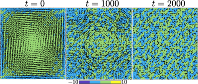
Figure 1: Snapshots of the velocity (represented by arrows) and vorticity (represented by colors) fields at $t=0,1000$, and $2000$ LJ units in our MD simulation with a vortex structure embedded in a noisy environment as an initial condition. The system evolves from an ordered structure ($t=0$) to a thermalized state ($t=2000$).

We start with randomly and homogeneously distributed particles with random velocities corresponding to 100 LJ temperature units. During the evolution, we solve the equation of motion for each particle, $m\ddot{\textbf{r}}_{i}=\ -\nabla\sum\phi_{ij}$, using the velocity-verlet algorithm with a time step of $dt=0.001$ LJ unit. We attach the system of particles to a Nosé-Hoover thermostat and let the particles attain thermal equilibrium, which takes around 100 LJ time units. We then remove the thermostat and allow the system to evolve as a micro-canonical ensemble for another 100 time units to remove the possibilities of any available free energy due to numerical or equilibration issues. The energy fluctuations in the asymptotic state are approximately $10^{-4}\%$. In the above thermalized state, we add the velocity of the coherent vortex of Eq. (2). This is the initial condition ($t=0$) for the non-equilibrium MD run.

After applying the vortex velocity profile, we let the LJ gas evolve from $t=0$ to $2000$ LJ units, approximately 56 eddy turnover time. In Figure 1, we illustrate three snapshots of the flow using the velocity and vorticity fields at $t=0$, 1000, and 2000 LJ time units. These plots illustrate the evolution from an ordered state to a thermalized state, consistent with the numerical results of 3D Euler turbulence Cichowlas et al. (2005b); Verma and Chatterjee (2022). We quantify the thermalization process using the kinetic energy spectrum and flux related to the hydrodynamic velocity. For the same, we compute the coarse-grained flow velocity ${\bf u(x},t)$ for a given snapshot by averaging over several hundred particles over a 40x40 grid. We Fourier transform ${\bf u(x},t)$ and compute ${\bf u(k},t)$, and subsequently, the modal energy $E({\bf k},t)=|{\bf u(k},t)|^{2}/2$. After this, we compute the 1D shell spectrum $E(k,t)=\sum_{k-1\leq k^{\prime}\leq k}E({\bf k}^{\prime},t)$ (Frisch, 1995). Our spectral plots exclude $E(k,t)$ at $k={k_{0},2k_{0}}$. However, all the available wavevectors are considered for the computation of nonlinear transfer, energy fluxes, and enstrophy.

Figure 2 illustrates the energy spectra at $t=10,15$, and $25$ LJ units, whereas Fig. 3 at $t=20,50,500$, and $2000$ LJ units. In these plots, the smallest wavenumber corresponding to the large-scale vortex is $k_{0}=2\pi/L\approx 0.0125$, whereas $k_{\mathrm{max}}=40k_{0}\approx 0.5$. For the initial evolution, Fig. 2 exhibits $E(k,t)\propto k^{-3}$ for small wavenumbers, and $E(k,t)\propto k$ at large wavenumbers. The $k^{-3}$ energy spectrum is related to the vortex structure, as explained later. The latter energy spectrum ($\propto k$) illustrates thermalization of the system at large wavenumbers. At around $t=25$, $E(k,t)$ at small $k$’s starts to deviate from $k^{-3}$ scaling because of the energy transfers from the vortex structure to the fluctuations. We observe that $E(k,t)\propto k$ at $t=500$ (or $\sim 14$ eddy turnover time) and beyond, which is consistent with the thermalization time for 3D Euler turbulence Cichowlas et al. (2005b).

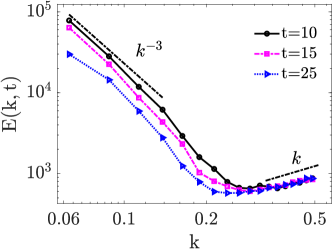
Figure 2: The shell spectra $E(k,t)$ of the LJ gas at $t=10,15$, and 25 LJ time units. Here, $E(k,t)\propto k^{-3}$ at small wavenumbers, and $E(k,t)\propto k$ at large wavenumbers. The latter $E(k,t)$ represents the thermalized component of the fluid.

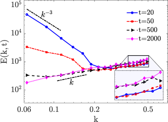
Figure 3: The shell spectra $E(k,t)$ of the LJ gas at $t=20,50,500$, and 2000 LJ time units. Here, $E(k,t)\propto k$ at 500 time units and beyond, indicating complete thermalization of the fluid. The inset shows that the amplitude of the thermalized $E(k,t)$ increases with time.

Figures 2 and 3 illustrate that the region of $k^{-3}$ spectrum shrinks with time, whereas that of $k$ spectrum increases with time. In addition, the magnitude of $E(k,t)$ decreases for small and intermediate wavenumbers, but it increases for large wavenumbers, similar to the evolution of 3D Euler turbulence Cichowlas et al. (2005a) (refer to the inset of Fig. 3). We denote the transition wavenumber between the $k^{-5/3}$ and $k$ regimes by $k_{c}$ and quantify the coherent and incoherent energies of the hydrodynamic component using $\sum_{k_{\mathrm{min}}}^{k_{c}}E(k,t)$ and $\sum^{k_{\mathrm{max}}}_{k_{c}}E(k,t)$ respectively. We illustrate these quantities in Fig. 4. Clearly, $k_{c}$ decreases with time because of the expansion of the $k$ spectrum at the cost $k^{-3}$ spectrum. Here, the system exhibits nonequilibrium behavior at large scales and equilibrium features at small scales. At $t=500$ LJ units, the coherent energy is nearly over, indicating nearly complete thermalization of the system. Note that the velocity follows the Maxwell-Boltzmann distribution; thus, local thermal equilibrium is always maintained. This feature deviates from the Euler turbulence that lacks the thermal component.

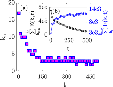
Figure 4: The time evolution of the transition wavevector $k_{c}$ that separates the coherent hydrodynamic energy (with $k^{-3}$ spectrum) and incoherent hydrodynamic energy (with $k$ spectrum). Note that $k_{c}$ decreases with time, as in Figs. 2 and 3. The inset exhibits a decrease in the total coherent energy $\sum_{k_{\mathrm{min}}}^{k_{c}}E(k,t)$ (black curve) and a growth in the total incoherent energy $\sum^{k_{\mathrm{max}}}_{k_{c}}E(k,t)$ (blue curve).

Next, we compute the energy and enstrophy transfers and the corresponding fluxes. Using the energy equation we derive that $dE(k,t)/dt=T^{E}(k,t)$, where $T^{E}(k,t)=\sum_{\bf p}\Im[\{{\bf k}\cdot{\bf u(k-p},t)\}\{{\bf u(p},t)\cdot{\bf u^{*}(k},t)\}]$ is the nonlinear energy transfer term, and that $\Pi^{E}(k)=-\int_{0}^{k}T^{E}(k^{\prime})dk^{\prime}$ Dar et al. (2001); Verma (2019b). In addition, the enstrophy, $\Omega=\int_{0}^{\infty}dk^{\prime}k^{\prime 2}E(k^{\prime})$, is conserved in Euler turbulence. Hence, $dE^{\Omega}(k,t)/dt=T^{\Omega}(k,t)=k^{2}T^{E}(k,t)$ and $\Pi^{\Omega}(k,t)=-\int_{0}^{k}T^{\Omega}(k^{\prime},t)dk^{\prime}=-\int_{0}^{k}k^{\prime 2}T^{E}(k^{\prime},t)dk^{\prime}$ Verma (2019b). Note that $\Pi^{E}(k,t)$ [$\Pi^{\Omega}(k,t)$] represents the net energy [enstrophy] transfer from the modes inside the wavenumber sphere of radius $k$ to the modes outside the sphere.

We compute $T^{E}(k,t)$, $T^{\Omega}(k,t)$, $\Pi^{E}(k,t)$, and $\Pi^{\Omega}(k,t)$ for our system. We estimate $T^{E}(k,t)\approx[E(k,t=25)-E(k,t=10)]/(2\times 7.5)$ with an optimum value of $\Delta t=7.5$ LJ units or 0.2 eddy turnover time. The above $\Delta t$ appears large, but it is reasonable considering large fluctuations in MD simulations. In Fig. 5, we plot $T^{E}(k,t)$, $T^{\Omega}(k,t)$, $\Pi^{E}(k,t)$, and $\Pi^{\Omega}(k,t)$. As shown in the figure, $T^{E}(k,t),T^{\Omega}(k,t)<0$, indicating energy and enstrophy transfers from smaller wavenumbers to larger wavenumbers. This feature leads to positive energy and enstrophy fluxes, with $\Pi^{E,\mathrm{max}}\approx 166$, and $\Pi^{\Omega,\mathrm{max}}\approx 1.05$. Note that our MD simulation has an interesting feature that deviates from Euler turbulence. For Euler turbulence, $\int_{0}^{\infty}T^{E}(k^{\prime},t)dk^{\prime}=0$ and $\Pi^{E}(k,t)\rightarrow 0$ as $k\rightarrow\infty$. However, for MD simulations, $\int_{0}^{\infty}T^{E}(k^{\prime},t)dk^{\prime}<0$ and $\Pi^{E}(k,t)$ is finite at $k=k_{\mathrm{max}}$. This is because in MD simulations, the hydrodynamic modes at the grid level transfer energy to the thermal particles, which is absent in Euler turbulence that has no thermal particles.

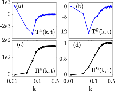
Figure 5: (a) Nonlinear energy transfer $T^{E}(k,t)$ and (b) nonlinear enstrophy transfer $T^{\Omega}(k,t)=k^{2}T^{E}(k,t)$. (c,d) The energy flux $\Pi^{E}(k,t)$ and the enstrophy flux $\Pi^{E}(k,t)$.

Lastly, we discuss the $k^{-3}$ energy spectrum exhibited in Figs. 2 and 3. The hydrodynamic velocity field till $t\lessapprox 20$ LJ units is reasonably well described by Eq. (2) with some added noise. For such a field configuration, the two-point correlation function $C({\bf r},t)=\langle{\bf u(x+r},t){\bf u(x},t)\rangle\propto\alpha-\beta r^{2}$, with $\alpha$ and $\beta$ as constants. Therefore, $C({\bf k},t)=\int d{\bf r}C({\bf r},t)\exp(i{\bf k\cdot r})\propto k^{-4}$, and hence $E(k,t)=C({\bf k},t)2\pi k\sim k^{-3}$. Interestingly, the above $k^{-3}$ spectrum is related to the Nastrom-Gage spectrum of Earth’s atmosphere at synoptic scales (1000-3000 km), which is coupled with $k^{-5/3}$ spectrum at mesoscales (10-500 km) Nastrom et al. (1984); Gage and Nastrom (1986). We remark that the above $k^{-3}$ spectrum is not directly related to Kraichnan’s predictions based on the constancy of enstrophy flux Kraichnan (1973a). Rather, it is connected to the large-scale 2D structures, as described above.

Researchers have constructed a variety of arguments to explain the Nastrom-Gage spectrum of Earth’s atmosphere Lindborg and Alvelius (2000); Tung and Orlando (2003); Gkioulekas and Tung (2006). Among the proposed theories, our results match best with the double cascade theory of Gkioulekas and Tung (2006). According to this theory, $E(k)\propto k^{-3}$ for $k<k_{t}$, whereas $E(k)\propto k^{-5/3}$ for $k>k_{t}$, where $k_{t}\approx\sqrt{\Pi^{\Omega,\mathrm{max}}/\Pi^{E,\mathrm{max}}}$ separates the two power law regimes. For our MD simulations, $k_{t}\approx 0.08$. Therefore, according to Gkioulekas and Tung (2006), we expect $k^{-3}$ energy spectrum for $k<k_{t}$ and $k^{-5/3}$ spectrum for $k>k_{t}$. Our simulation exhibits only the $E(k)\propto k^{-3}$ for $k<k_{t}$ because $k_{t}$ is close to the dissipation scale.

We summarize our results as follows. We simulate thermalization of a realistic fluid system containing a large number of weakly interacting particles that are also part of a large hydrodynamic vortex. We isolate our system from the heat bath so as to conserve the total energy. Thus, our system resembles Euler turbulence with energy-conserving noise. In the early phase, the system exhibits $E(k)\propto k^{-3}$ and $E(k)\propto k$ at small and large wavenumbers, respectively. The system gets fully thermalized at $t\gtrsim 500$ LJ units, at which point the coherent hydrodynamic energy is fully transferred to the incoherent hydrodynamic component ($E(k)\propto k$) and thermal noise. We strengthen our arguments using the energy and enstrophy transfers. Our MD simulation clearly demonstrates how large-scale kinetic energy cascades to small scales in a realistic turbulent system.

Our results are consistent with the route to thermalization observed earlier in Euler turbulence Cichowlas et al. (2005a), in Navier-Stokes equation with fluctuating hydrodynamics Bell et al. (2022); Bandak et al. (2022), and in DSMC simulations McMullen et al. (2022). However, there are some subtle differences. In our simulation, some of the hydrodynamic energy is transferred to the thermal particles at the microscopic level, which is absent in 3D Euler turbulence. We also remark that our MD simulations represent the particle dynamics more realistically than DSMC.

In our system, the large-scale initial structure generates $k^{-3}$ energy spectrum, as well as forward energy and enstrophy fluxes. Such dynamics resemble that in Earth’s atmosphere at the synoptic scales Gage and Nastrom (1986). A difference, however, is that the atmospheric vortex structures are maintained by large-scale forcing. However, the vortex structure in our system breaks down and thermalizes due to a lack of external forcing. Interestingly, in earlier simulations of 2D Euler systems with large-scale structures as initial conditions exhibit nonequilibrium behaviour Bouchet and Simonnet (2009); Bouchet and Venaille (2012); Verma and Chatterjee (2022). In contrast, the initial vortex structure in our 2D MD simulation thermalizes. However, we also found similar thermalization for other initial conditions such as sheared flow, wave excitation, Rayleigh-Taylor instability, and four-vortex during the validation process.

Thus, our MD simulations of hydrodynamic structures embedded in a noisy environment provide valuable insights into the thermalization process in a realistic fluid system. The work also sheds light on the connection between hydrodynamics and thermodynamics, which are active at macroscopic and microscopic scales, respectively.

Acknowledgements. The authors acknowledge the use of AGASTYA HPC for present studies. RW and ST also acknowledge the support for this work through SERB Grant No. CRG/2020/003653, and MKV the support of SERB Grant Nos. SERB/PHY/20215225 and SERB/PHY/2021473.

References

- Huang (2008) K. Huang, Statistical mechanics (John Wiley & Sons, 2008).
- Bellomo and Schiavo (1997) N. Bellomo and M. L. Schiavo, Mathematical and Computer Modelling 26, 43 (1997).
- Reif (1965) F. Reif, Fundamentals of Statistical and Thermal Physics (McGraw-Hill, New York, 1965).
- Goldstein (2001) S. Goldstein, in Chance in physics: Foundations and perspectives (Springer, 2001) pp. 39–54.
- Grad (1958) H. Grad, “Principles of the kinetic theory of gases,” (Springer Berlin Heidelberg, 1958).
- Loeb (2004) L. B. Loeb, The kinetic theory of gases (Courier Corporation, 2004).
- Gallis et al. (2017) M. A. Gallis, N. P. Bitter, T. P. Koehler, J. R. Torczynski, S. J. Plimpton, and G. Papadakis, Phys. Rev. Lett. 118, 064501 (2017).
- Bell et al. (2022) J. B. Bell, A. Nonaka, A. L. Garcia, and G. Eyink, J. Fluid Mech. 939, A12 (2022).
- Bandak et al. (2022) D. Bandak, N. Goldenfeld, A. A. Mailybaev, and G. Eyink, Phys. Rev. E 105, 065113 (2022).
- McMullen et al. (2022) R. M. McMullen, M. C. Krygier, J. R. Torczynski, and M. A. Gallis, Phys. Rev. Lett. 128, 114501 (2022).
- Cichowlas et al. (2005a) C. Cichowlas, P. Bonaïti, F. Debbasch, and M. Brachet, Phys. Rev. Lett. 95, 264502 (2005a).
- Lee (1952) T. D. Lee, Quart. Appl. Math. 10, 69 (1952).
- Kraichnan (1973a) R. H. Kraichnan, J. Fluid Mech. 59, 745 (1973a).
- Onsager (1949) L. Onsager, Il Nuovo Cimento 6, 279 (1949).
- Kolmogorov (1941a) A. N. Kolmogorov, Dokl Acad Nauk SSSR 30, 301 (1941a).
- Kolmogorov (1941b) A. N. Kolmogorov, Dokl Acad Nauk SSSR 32, 16 (1941b).
- Frisch (1995) U. Frisch, Turbulence: The Legacy of A. N. Kolmogorov (Cambridge University Press, Cambridge, 1995).
- Davis et al. (2001) M. J. Davis, S. A. Morgan, and K. Burnett, Phys. Rev. Lett. 87, 160402 (2001).
- Proment et al. (2009) D. Proment, S. Nazarenko, and M. Onorato, Phys. Rev. A 80, 051603 (2009).
- Barenghi et al. (2014) C. F. Barenghi, L. Skrbek, and K. R. Sreenivasan, Proceedings of the National Academy of Sciences 111, 4647 (2014).
- Betchov (1957) R. Betchov, J. Fluid Mech. 3, 205 (1957).
- Robert and Sommeria (1991) R. Robert and J. Sommeria, J. Fluid Mech. 229, 291–310 (1991).
- Kraichnan (1973b) R. H. Kraichnan, J. Fluid Mech. 59, 745–752 (1973b).
- Pakter and Levin (2018) R. Pakter and Y. Levin, Phys. Rev. Lett. 121, 020602 (2018).
- Bouchet and Simonnet (2009) F. Bouchet and E. Simonnet, Phys. Rev. Lett. 102, 094504 (2009), 0804.2231 .
- Seyler et al. (1975) C. E. Seyler, Y. Salu, D. Montgomery, and G. Knorr, Physics of Fluids 18, 803 (1975).
- Verma and Chatterjee (2022) M. K. Verma and S. Chatterjee, Phys. Rev. Fluids 7, 114608 (2022).
- Bouchet and Venaille (2012) F. Bouchet and A. Venaille, Phys. Rep. 515, 227 (2012).
- Verma et al. (2020) M. K. Verma, S. Bhattacharya, and S. Bhattacharya, arXiv , arXiv:2004.09053 (2020).
- Martinez et al. (1994) D. O. Martinez, W. H. Matthaeus, S. Chen, and D. C. Montgomery, Phys. Fluids 6, 1285 (1994).
- Chen and Doolen (1998) S. Chen and G. D. Doolen, Annual review of fluid mechanics 30, 329 (1998).
- Bird (1976) G. A. Bird, NASA STI/Recon Technical Report A 76, 40225 (1976).
- Kadau et al. (2004) K. Kadau, T. C. Germann, N. G. Hadjiconstantinou, P. S. Lomdahl, G. Dimonte, B. L. Holian, and B. J. Alder, Proc. Natl. Acad. Sci. 101, 5851 (2004).
- Ashwin and Sen (2015) J. Ashwin and A. Sen, Phys. Rev. Lett. 114, 055002 (2015).
- Wani et al. (2022) R. Wani, A. Mir, F. Batool, and S. Tiwari, Scientific Reports 12 (2022).
- Cichowlas et al. (2005b) C. Cichowlas, P. Bonaïti, F. Debbasch, and M. E. Brachet, Phys. Rev. Lett. 95, 264502 (2005b).
- Verma (2019a) M. K. Verma, Eur. Phys. J. B 92, 190 (2019a).
- Verma (2020) M. K. Verma, Phil. Trans. R. Soc. A. 378, 20190470 (2020).
- Plimpton (1995) S. Plimpton, Journal of Computational Physics 117, 1 (1995).
- Dar et al. (2001) G. Dar, M. K. Verma, and V. Eswaran, Physica D 157, 207 (2001).
- Verma (2019b) M. K. Verma, Energy transfers in Fluid Flows: Multiscale and Spectral Perspectives (Cambridge University Press, Cambridge, 2019).
- Nastrom et al. (1984) G. Nastrom, K. Gage, and W. Jasperson, Nature 310, 36 (1984).
- Gage and Nastrom (1986) K. S. Gage and G. D. Nastrom, J. Atmos. Sci. 43, 729 (1986).
- Lindborg and Alvelius (2000) E. Lindborg and K. Alvelius, Phys. Fluids 12, 945 (2000).
- Tung and Orlando (2003) K.-K. Tung and W. W. Orlando, J. Atmos. Sci. 60, 824 (2003).
- Gkioulekas and Tung (2006) E. Gkioulekas and K.-K. Tung, Journal of Low Temperature Physics 145, 25 (2006).