SCADI: Self-supervised Causal Disentanglement
in Latent Variable Models

Abstract

Causal disentanglement has great potential for capturing complex situations. However, there is a lack of practical and efficient approaches. It is already known that most unsupervised disentangling methods are unable to produce identifiable results without additional information, often leading to randomly disentangled output. Therefore, most existing models for disentangling are weakly supervised, providing information about intrinsic factors, which incurs excessive costs. Therefore, we propose a novel model, SCADI(SElf-supervised CAusal DIsentanglement), that enables the model to discover semantic factors and learn their causal relationships without any supervision. This model combines a masked structural causal model (SCM) with a pseudo-label generator for causal disentanglement, aiming to provide a new direction for self-supervised causal disentanglement models.

1 Introduction

Imitating humans has been the ultimate goal of machine learning, and now machine learning is capable of performing various tasks. However, due to the inherent drawbacks of black box models, there are still limitations in understanding and learning complex relationships. To imitate image understanding of human, we consider a two-step process, as depicted in Fig. 1. The first step is observation, learning about the various elements presented in the data, such as light sources, a swinging pendulum, and shadows (see Fig. 1). The second step is interpretation, which involves understanding the relationships among the elements identified during the observation stage. This paper aims to propose a methodology that can perform both observation and interpretation without any supervision. Our approach, SCADI (Self-supervised Causal Disentanglement), is based on disentangled representation learning, and brings us closer to the process of human thinking. Disentangling aims to understand the factors of variation in the data, and can compress complex data in a concise and information-rich manner, making it beneficial for downstream tasks [1, 2, 3, 4, 5, 6, 7]. The early-stage disentangling was done through unsupervised learning using latent variable models with an independence assumption on factors, such as variational autoencoders (VAEs)[8, 9, 10, 11]. Among them, $\beta$-VAE [8][12] serves as our baseline model for observer. $\beta$-VAE adjusts the balance between the reconstruction loss and the Kullback-Leibler (KL) divergence in the objective function. Minimizing the KL divergence loss, weighted by $\beta$, enforces independence among factors by encouraging the latent variables to align with the prior distribution. However, Locatello et al.[13] demonstrated that unsupervised disentangling lacks identifiability [14], making it difficult to get consistent results. As a result, many weakly supervised disentangling models emerged [15][16][17][18] [19], which incorporate additional information or inductive biases . Nevertheless, the cost of the labels is excessive. Therefore, various semi-supervised disentangling approaches have been proposed[20] [21] [22] [23], with many still maintaining the independence assumption. However, feature independence is often unrealistic (Fig. 1). Consequently, models such as CausalGAN[24], CausalVAE[25], and DEAR[26] have emerged, which have discarded the independence assumption, but they still provide additional information in the form of labels[25] or by incorporating prior causal graphs [24][26], or using weakly paired datasets[27]. DEAR[26] aims to utilize a practical amount of labeled data, but it requires prior knowledge about causal graph.

To significantly alleviate the burdens of supervision, we propose the first self-supervised approach that prevents random disentanglement. In our best knowledge, SCADI(Self-supervised CAusal Disentanglement), is the first attempt at achieving causal structured disentanglement without any additional information or inductive biases. SCADI has two main components: 1. An observer, which performs dimension-wise unsupervised disentangling through a latent variable model, generating pseudo-labels. 2. An interpreter, a module for vector-wise weakly supervised causal disentanglement. It relies on the structured causal model (SCM) [28, 29]. SCM has played a significant role in incorporating causality into latent variable models[26][30][31][24], including in CausalVAE[25], which serves as the baseline for interpreter. In SCADI, the interpreter is supervised by the labels generated by the observer, while the observer receives additional regularization from the interpreter, which forces the adjacency matrix in masked SCM to be a directed acyclic graph (DAG). Our detailed explanations and experiments address how SCADI performs causal disentanglement. Our code is available at https://github.com/Hazel-Heejeong-Nam/Self-supervised-causal-disentanglement.

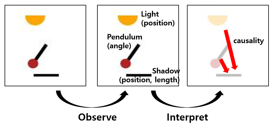
Figure 1: Process of understanding image : Observation and Interpretation.

2 Method

Starting with observer, we adopt a latent variable model for unsupervised disentangling, $\beta$-VAE[8], to utilize the latent space as pseudo-labels. While $\beta$-VAE, does not capture causality directly, its KL divergence forces it to focus on the most distinguishable features in data. However, as highlighted by Locatello et al.[13], unsupervised disentangling models not only cannot always produce well-disentangled results, but also lack the ability to disentangle correlated factors. This prompted us to consider providing additional regularization to improve the quality of the pseudo-labels.

Definition 1 (Symbols of our model). We will begin by defining our notations. $\hat{g}(\cdot)$ and $g(\cdot)$ will be also explained further in 2

• Dataset $X$ consists of $n$ images. i.e. $X:=\{x_{1},...,x_{n}\}$, where $x_{i}\in\mathbb{R}^{W\times H\times C}$.

• Adjacency Matrix $\mathbb{A}:=\{A_{1},...,A_{n}\}$, where $A_{i}:=[A_{i}^{1}|...|A_{i}^{c}]$ and $A_{i}^{jk}:=\{A_{i}^{jk}\}_{k=1}^{c}$. $c$ is the number of factors of interest in data.

• Exogenous latent variables are $E:=\{\epsilon_{1},...,\epsilon_{n}\}$, where $\epsilon_{i}:=f(x_{i})$. $f(\cdot)$ is the first encoder in Fig.2. $\epsilon_{i}\in\mathbb{R}^{\alpha\cdot c}$ where $\alpha$ is an arbitrary positive number. Endogenous latent variables are $z_{i}=\hat{g}(A_{i},\epsilon_{i})$ , $z_{i}\in\mathbb{R}^{c\times\alpha}$and $Z:=\{z_{1},...z_{n}\}$, where $z_{i}^{jk}$ is value of $j^{th}$ row and $k^{th}$ column in $z_{i}$.

• Observed Labels are $U:=\{u_{1},...,u_{n}\}$, where $u_{i}:=f_{O}(\epsilon_{i})$, are defined as observed labels from Observer. $f_{O}$ is an additional observation encoder followed by the shared encoder, and $u_{i}:=\{u_{i}^{k}\}_{k=1}^{c}$.

• Decoders : Observation decoder and interpretation decoder are denoted as $h_{O}(\cdot)$ and $h_{I}(\cdot)$ respectively. We define reconstructed data as $\tilde{x_{i}}_{O}:=h_{O}(u_{i})$ and $\tilde{x_{i}}_{I}:=h_{I}(g(A_{i},z_{i})$

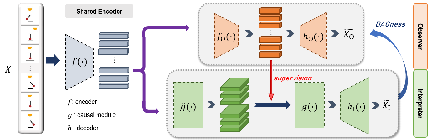
Figure 2: Overview of self-supervised structured causal disentanglment.

Example 1 . We additionally define true underlying factor set $S$ with $c$ factors in it, i.e. $S:=\{s^{1},...,s^{c}\}$. Any pair of $(s^{i},s^{j})$ can be either independent or causally related. Fig. 3 (a) shows an entangled case of the observer’s disentangling process. Both observed factors $u^{i}$ and $u^{j}$ are having combined effects of true factors $s^{i}$ and $s^{j}$. Here, we assume $i^{th}$ factor is a cause of $j^{th}$ factor, i.e. $i^{th}$ factor and $j^{th}$ factor are in parent-child relationship. Successful disentanglement would make the distributions of true underlying factor $S$ and observed factor $U$ aligned.

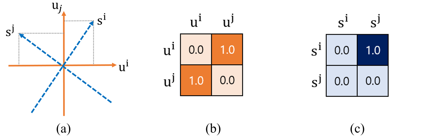
Figure 3: (a) Observed factors and true underlying factors are entangled. (b) Adjacency matrix of observation. (c) Adjacency matrix of true factors.

We incorporate the concept of DAGness[25, 32, 33] in the adjacency matrix for SCM, denoted as $H(A)$ in (1). After the labels were passed to the interpreter, SCADI performs causal disentangling within SCM and learns $A$. In Example 1, $A$ of true underlying factors should be like Fig.3(c). However, if the generated labels are entangled, as shown in Fig.3(a), $A$ would exhibit bidirectional relationships, as in Fig.3(b). Therefore DAGness of $A$ can assess the disentanglement in observer, and in the same context, minimize DAGness would assist disentangling factors by helping to suppress bidirectional relationships and anchor the factors in place. Although this constraint does not yet achieve complete mathematical identifiability[14], we insist that DAGness prevents randomly disentangled results in the observer. The proved identifiability of the CausalVAE[25], corresponding to our interpreter, implies that if only the generated labels are well-disentangled, the identifiability of SCADI will also be satisfied.

$$H(A)\equiv tr((I+A\circ A)^{c})-c$$ (1)

Observer and Interpreter

The task of the observer is to provide a scalar label for each factor. Observer has two key differences from $\beta$-VAE[8]. Firstly, it undergoes a two-step encoding process. In the first encoding step, $f(\cdot)$ shares its weights and the latent space with the interpreter. The exogenous latent vector $E$ from $f(\cdot)$ does not inherently encode relationships among factors. In the second step, the output vector $U$ with a fixed length $c$ is obtained through $f_{O}(\cdot)$. $U$ is not only fed to the decoder $h_{O}(\cdot)$ but also serves as the label passed to the interpreter. Finally, by adding the evidence lower bound (ELBO) loss, the objective function of the observer can be written as (2).

$$L_{obs} =-\mathbb{E}_{q_{\phi}(u|x,\epsilon)}[\log p_{\theta}(x,\epsilon|u)]+w_{O}^{d}H(A)+\beta D_{KL}(q_{\phi}(u|x,\epsilon)||p_{\theta}(u))$$

$$=-\text{ELBO}+w_{O}^{d}H(A)$$ (2)

The interpreter is similar to CausalVAE[25], which adopts SCM. The exogenous latent variable $E$ is mapped to the endogenous latent variable $Z$ through causal inference, using the adjacency matrix $A$. Here, a linear SCM[28] equation, as shown in (3), is employed. We defined (3) as $\hat{g}$. Subsequently, SCADI performs causal disentanglement within the masked SCM[29]. By masking out non-parental elements of $Z$ using $A$ in each semantic vector, the model is able to learn the effects of the individual factors while maintaining their connections with their parental semantics. This can be written as (4), where $j$ represents each concept and $a$ is a non-linear function for stability. We defined (4) as $g$, where $\eta_{i}$ is the parameter set of $a$.

$$z=A^{T}z+\epsilon=(I-A^{T})^{-1}\epsilon,\quad\epsilon\sim N(0,I)$$ (3)

$$z^{j}=a^{j}(A^{j}\odot z;\eta^{j})+\epsilon^{j}$$ (4)

$$u^{j}=a^{j}(A^{j}\odot u;\eta^{j})$$ (5)

In Similar way, the labels generated from the observer are fed to the SCM layer as (5). The mask loss, denoted as $l_{m}$, compares $z$ before and after applying (4), and then incorporated into the objective function of the interpreter. Similarly, the label loss, $l_{u}$, can be obtained by comparing $u$ before and after the mask layer. Adding evidence lower bound (ELBO) loss, the interpreter loss can be described as (6). We follow Yang et al.[25] for further details. To summarize, the observer receives DAGness from the interpreter, while the interpreter obtains labels from the observer, establishing a mutually beneficial relationship. During training, in order for all parameters to be updated at least once, two forward passes are needed. The first pass aims to minimize the objective function for the observer(2), as illustrated by the gradient flow depicted in Fig.4(a). The second forward pass aims to minimize the objective function for the interpreter(6), and we detach the gradient of the label as in Fig.4(b). During inference, only a single forward pass is required.

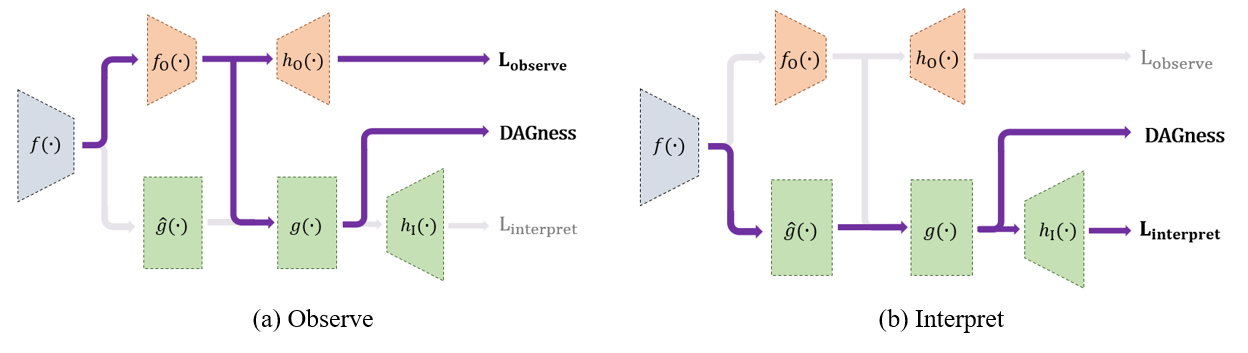
Figure 4: Gradient flow while training observer and interpreter.

$$L_{int} =-\mathbb{E}_{\epsilon,z}[\log p_{\theta}(x|z,\epsilon,u)]+D_{KL}(q_{\phi}(\epsilon,z|x,u)||p_{\theta}(\epsilon,z|u))+w_{I}^{d}H(A)+w_{I}^{u}l_{u}+w_{I}^{m}l_{m}$$

$$=-\text{ELBO}+w_{I}^{d}H(A)+w_{I}^{u}l_{u}+w_{I}^{m}l_{m}$$ (6)

3 Experiments

Synthetic pendulum dataset  We utilized the synthetic pendulum dataset by Yang et al. [25]. Each image consists of a light source, a pendulum, and a shadow with varying lengths and locations determined by the position of the light source and pendulum. The factor of variants are as follows[25][26] : 1) pendulum angle, 2) light position, 3) shadow length, and 4) shadow position. With the official split of the train and test set[25], we obtained 5482 training images and 1826 test images. Fig.8(b) shows the true causal graph of the described factors.

Baselines We compared our model with 3 differenct architectures: CausalVAE[25], unsup-CausalVAE[25], and nd-SCADI. Unsup-CausalVAE eliminates supervision from the masked SCM as Yang et al.[25] did, which is equivalent to using only interpreter in SCADI. Nd-SCADI is a modified model from SCADI, which abandoned extra DAGness regularization to the observer. Table 1 shows differences among SCADI and its baselines. We also provide brief structures of our baselines in Appendix B.

[] Supervision Observer Interpreter CausalVAE[25] $\circ$ $\times$ $\circ$ unsup-CausalVAE[25] $\times$ $\times$ $\circ$ nd-SCADI $\times$ $\circ$ $\circ$ SCADI $\times$ $\circ$ $\circ$

Table 1: Baselines and architecture summary

3.1 Setup and evaluation

For the observer in SCADI, we assess how well the model separates the factors. In existing weakly supervised methods, providing supervision makes it easier to determine which dimension of the latent space encodes a specific underlying factor. However, since unsupervised disentangling does not have a predefined order in the latent vector, it becomes essential to reveal the order of the factors for further interpreter analysis. To do so, we categorized a small subset of counterfactual images, twice the number of factors, as the label-finding set depicted in Figure 5. We then used these images to examine which factors are encoded in each dimensions of the latent vector produced by observer.

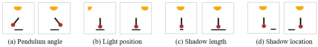
Figure 5: Label-finding set. (a),(b),(c),(d) are showing paired data for corresponding factors.

Definition 2 (Label-Finding process).  As shown in Fig. 5, the label-finding set is divided into subgroups. Each subgroup consists of a pair of counterfactual images, $(F_{a}^{i},F_{b}^{i})$, which differ only in the state of the $i^{th}$ semantic, while the other semantics remain the same. By calculating the absolute element-wise difference between the latent variables generated from $F_{a}^{i}$ and $F_{b}^{i}$, we can quantify the variation in each dimension when the $i^{th}$ semantic changes. We consider the index of the latent variable with the largest difference as $label_{i}$, since the $i^{th}$ value in the latent vector strongly encodes the $i^{th}$ semantic. (7) summarizes the label-finding process, where obs denotes the observation process of getting the labels.

Definition 3 (Label-Quality score).  We defined the LQ(Label-Quality) score measured based on Label-Finding process. We calculate cross-entropy loss between label and $|obs(F_{a}^{i})-obs(F_{b}^{i})|$. Eq. (8) shows how LQ score is calculated. We consider a lower LQ score to indicate better performance.

$$label_{i}=\text{max}(|obs(F_{a}^{i})-obs(F_{b}^{i})|)$$ (7)

$$lq_{i}=\text{Cross Entropy}(|obs(F_{a}^{i})-obs(F_{b}^{i})|,label_{i})$$ (8)

We prioritize non-overlapping labels. Even if the LQ score is better, overlapped labels indicate suboptimal performance. Our evaluation enables an examination of how semantics are represented and how strongly they are disentangled. For the evaluation of the interpreter, we followed CausalVAE[25]. Quantitatively, we examine the DAGness where a smaller DAGness indicates a less entangled result. Qualitatively, we first directly compared the obtained causal graph to the ground truth. While each value in $A$ ranges from 0 to 1, we rounded up to determine causality. Secondly, since most of the casual disentangling models are generative latent variable models[25, 24, 26, 31], learned causality can be visualized through do-operations[26][25], which intervene on latent variables to generate counterfactual data [34]. Ideally, if the parent element is changed, the corresponding child also should be changed accordingly, while the parent element should remain unaffected even though the child element has been changed. See Appendix A for our implementation details.

3.2 Experiment results

captionskip=4pt [] Intervene $u[0]$ $u[1]$ $u[2]$ $u[3]$ shadow length 1.6296 0.9784 0.1379 0.5790 light 7.0160 6.8370 3.3080 0.3135 pendulum 2.6932 0.9545 3.6941 2.8357 shadow location 0.7641 0.1960 1.8232 3.3046

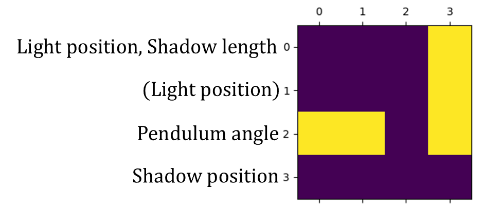
Figure 6: Label finding process

[]

Figure 7: Adjacency matrix of SCADI

Observation and interpretation

Table 7 shows $|obs(F_{a}^{i})-obs(F_{b}^{i})|$ of SCADI while intervening each factor. Pendulum angle and shadow location are fully disentangled in $u[2]$ and $u[3]$ respectively, having the same largest value both in row and column. However, shadow length and light position have the largest value in $u[0]$ in their row, thus seem to be entangled. Even though they are not fully disentangled, column $u[1]$ strongly encodes light position. Consequently, we labeled each latent dimension as Fig.7. Then we compare our obtained result (Fig. 8 (a)) to the true causal graph (Fig. 8 (b)). We found that SCADI can capture causal relationship to some extent in a cost-effective manner. Fig. 8 (c) demonstrates that SCADI generates strong labels which are able to reconstruct counterfactual images by do-operation. In detail, A and C intervene light position and pendulum angle respectively, which are both parental elements of the shadow position and length. Thus, the position and length of the shadow changed as a result of do-operation. However, in B and D, the length and center location of the shadow are changed respectively, which are not parental elements for none of the others. Thus, even when shadow labels are intervened, the other factors remain the same.

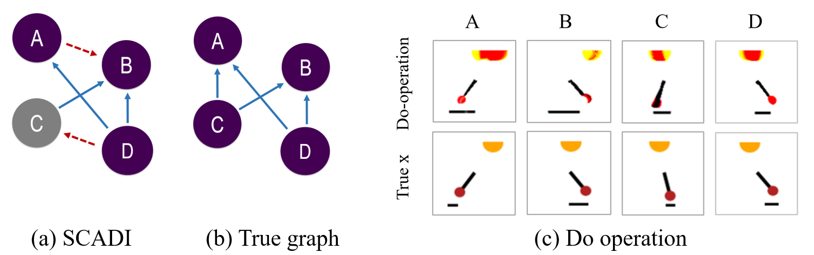
Figure 8: For simplicity, following symbols are used: A for the shadow length, B for the light position, C for the pendulum angle, and D for the shadow location. (a) Graph based on Fig. 7. Red arrows indicate a incorrect causal relationship. C is ambiguous in the result of SCADI. (b) True causal graph. (c) Result of do-operation. To lessen ambiguity, the A is considered to be in $u[0]$ and C is in $u[1]$.

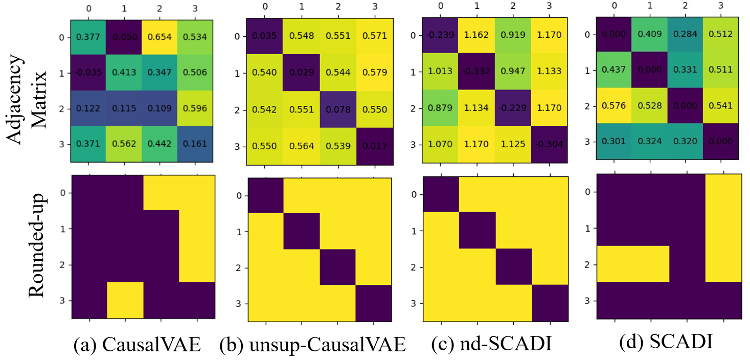
Figure 9: Comparison of the adjacency matrices of various unsupervised models.

Comparative Evaluation

Fig.9 illustrates the final adjacency matrices of four models (Table 1), including SCADI. It is evident that the unsup-CausalVAE and nd-SCADI exhibit subpar performance, as evidenced by the full entanglement within adjacency matrix. In contrast, CausalVAE with weak supervision and SCADI with self-generated labels show adjacency matrices that nearly satisfy and fully satisfy the Directed-Acyclic-Graph (DAG) conditions, respectively. Furthermore, upon comparing the obtained relationships and the ground truth, both SCADI and the reproduced CausalVAE successfully capture major causality among the factors. (See Fig.8 for SCADI, and Appendix B for CausalVAE.) Additionally, Table 3 shows DAGness of $A$ after training, indicating that SCADI, trained to ensure DAG in both the observer and interpreter, exhibits the lowest DAGness.

Subsequently, we compute the LQ scores for SCADI and nd-SCADI, which are equipped with an observer structure (See Table 1.). As shown in Table 3, SCADI, with additional DAGness imposed on the observer, demonstrated a higher average LQ score in comparison to nd-SCADI. This observation suggests that DAGness aids the observer in anchoring its labels to the underlying factors effectively.

captionskip=4pt [0.7] factor of variation average LQ shad length ligth pos pendulum shad loc nd-SCADI $u$ index 3 0 2 3 0.6744 LQ 0.5915 0.4901 0.6485 0.9675 SCADI $u$ index 0 0 2 3 0.5698 LQ 0.7401 0.6216 0.6167 0.3007

Table 2: Evaluation of unsupervised causal disentanglement methods

[] DAGness CausalVAE 0.5298 unsup-CausalVAE 0.4745 nd-SCADI 9.7837 SCADI 0.1359

Table 3: Final DAGness

4 Conclusion

In conclusion, this paper has endeavored to propose a methodology capable of conducting both observation and interpretation in an unsupervised manner. SCADI is able to capture major causality among factors effectively, and showed better disentanglement result than the other fully unsupervised settings. We hope that our work contributes to future research that aims to achieve unsupervised causal disentanglement.

Appendix A Implementation details

We assign a 16-dimension latent space ($\alpha=4,c=4$) for the output of the shared encoder. A batch size of 512 and 500 epochs for training are chosen as default. Adam optimizer is adopted with a learning rate of 0.001 for the observer and 0.0003 for the interpreter. The default DAG constraint for the observer is set to $6H(A)+1H(A)^{2}$, which is twice as large as the DAG constraint used in the interpreter, i.e. $3H(A)+0.5H(A)^{2}$ is used for interpreter which is a default setting of CausalVAE[25]. The $\beta$ parameter for the observer is set to 20, while the default setting for the interpreter is 4[25]. Every network in the model consists of linear layers with the ELU[35] activation functions as CausalVAE[25] did. Details of the encoder and decoder architectures are shown in Table 11 and Table 11. We followed Yang et al.[25] for further details.

captionskip=4pt [] Shared encoder Observation encoder Linear$(W*H*C,900)$ Linear$(\alpha*c,\alpha*c)$ ELU( ) ELU( ) Linear$(900,300)$ Linear$(\alpha*c,\alpha*c)$ ELU( ) ELU( ) Linear$(300,2*\alpha*c)$ Linear$(2*c)$

Figure 10: Encoders

[] Observation decoder Interpreteration decoder^a Linear$(c,300)$ Linear$(\alpha,300)$ ELU( ) ELU( ) Linear$(300,300)$ Linear$(300,300)$ ELU( ) ELU( ) Linear$(300,1024)$ Linear$(300,1024)$ ELU( ) ELU( ) Linear$(1024,1024)$ Linear$(1024,W*H*C)$ ELU( ) Linear$(1024,W*H*C)$ ^a Each factor has seperated interpreter decoder, i.e. Total number of interpreter decoder SCADI has is $c$.

Figure 11: Decoders

Appendix B Experiment details

While our default training duration comprised 500 epochs, the progress of learning the adjacency matrix $A$ is illustrated in Fig. 12. In Epoch 0, we initialize the diagonal elements to 0 and all the others to $0.5$ so that initialized matrix $A$ looks like Fig.12 (a) after rounding up. Fig.12(b) still has a bidirectional relationship, but it almost satisfies a DAG. After more iterations, Fig.12 (c) and (d) satisfy DAG.

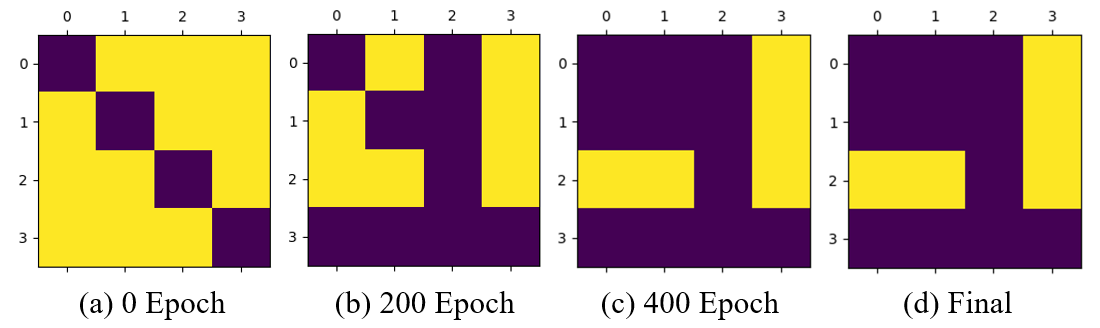
Figure 12: Progress of learning adjacency matrix.

During our experiment in Section3.2, four different structures were compared, and Fig.13 briefly shows the differences among them.

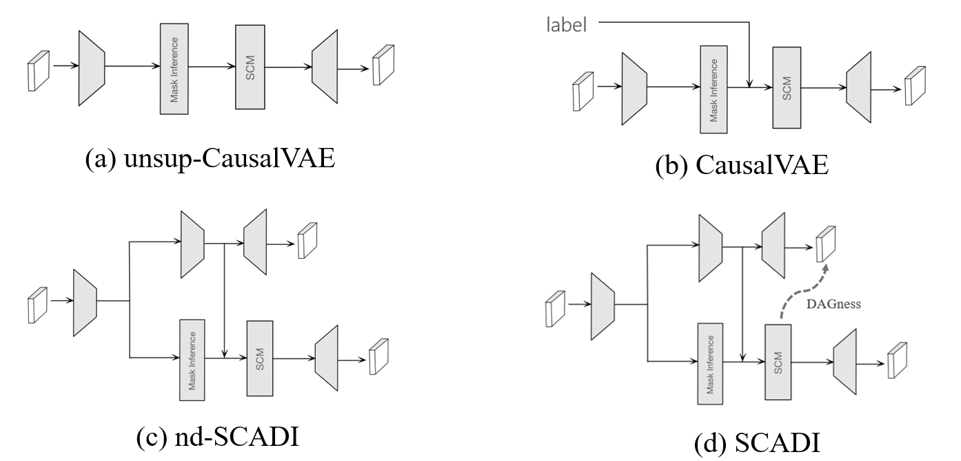
Figure 13: Architectures used in Sec.3.2

Furthermore, Fig 14 shows additional results from the reproduced CausalVAE[25]. As it operates with weakly supervised labels, there is no need for a label-finding process. The order of factors in the latent variable is predefined: arranged as pendulum angle, light position, shadow length, and shadow location. During the reproduction of CausalVAE results, we referenced the default settings proposed by Yang et al.[25]. While not in perfect alignment with the ground truth, it is discernible that the model successfully captured significant causality among the factors.

Figure 14: Additional anaylsis on CausalVAE

Appendix C Ablation study on DAGness

This experiment aims to investigate whether the additional regularization imposed on the observer, referred to as DAGness, leads to the generation of higher-quality labels. To investigate the impact of varying levels of DAGness on causal disentangling, we conducted an experiment by giving different conditions: 1) No DAGness to the observer, 2) Half the amount of DAGness compared to our default setting, and 3) SCADI with the default setting. Table 4 shows quantitative result and Fig. 15 shows the adjacency matrices.

[] factor of variation average LQ DAGness shad length light pos pendulum shad loc $0H(A)+0H(A)^{2}$ $u$ index 3 0 2 3 0.6744 9.7387 LQ 0.5915 0.4901 0.6485 0.9675 $3H(A)+0.5H(A)^{2}$ $u$ index 0 0 0 3 0.7581 0.0942 LQ 1.0366 0.3373 1.3862 0.2755 $6H(A)+H(A)^{2}$ $u$ index 0 0 2 3 0.5698 0.1359 LQ 0.7401 0.6216 0.6167 0.3007

Table 4: Overall results with varying degree of DAGness

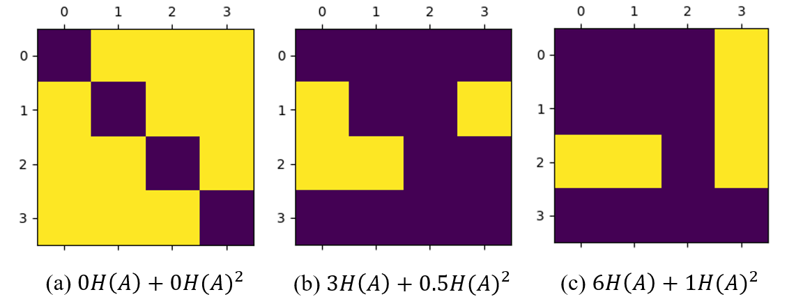
Figure 15: Comparing the adjacency matrices with varying degrees of DAGness

In SCADI without imposing DAGness on the observer, all factors are causallly entangled, as can be seen in Fig.15, even though labels from label-finding process do not overlap significantly. This indicates that the observer could not generate strong labels without DAGness , meaning that the factors are not anchored to the distribution of the true underlying factors. Imposing half the amount of DAGness allows the observer to generate a directed acyclic adjacency matrix. However, Table 4 shows that the underlying factors are poorly disentangled, showing overlapped labels in the observed latent space. SCADI with a proper amount of DAGness not only has a directed acyclic adjacency matrix but also has the best average LQ score, indicating that both the observer and interpreter operate well.

References

- [1] Yoshua Bengio, Aaron Courville, and Pascal Vincent. Representation learning: A review and new perspectives, 2014.
- [2] Yann LeCun, Y. Bengio, and Geoffrey Hinton. Deep learning. Nature, 521:436–44, 05 2015.
- [3] Ian Goodfellow, Honglak Lee, Quoc Le, Andrew Saxe, and Andrew Ng. Measuring invariances in deep networks. In Y. Bengio, D. Schuurmans, J. Lafferty, C. Williams, and A. Culotta, editors, Advances in Neural Information Processing Systems, volume 22. Curran Associates, Inc., 2009.
- [4] Francesco Locatello, Gabriele Abbati, Tom Rainforth, Stefan Bauer, Bernhard Schölkopf, and Olivier Bachem. On the fairness of disentangled representations, 2019.
- [5] Raphael Suter, Ðorðe Miladinovic, Stefan Bauer, and Bernhard Schölkopf. Interventional robustness of deep latent variable models. ArXiv, abs/1811.00007, 2018.
- [6] Irina Higgins, David Amos, David Pfau, Sebastien Racaniere, Loic Matthey, Danilo Rezende, and Alexander Lerchner. Towards a definition of disentangled representations, 2018.
- [7] Léon Bottou, Olivier Chapelle, Dennis DeCoste, and Jason Weston. Scaling Learning Algorithms toward AI, pages 321–359. 2007.
- [8] Irina Higgins, Loïc Matthey, Arka Pal, Christopher P. Burgess, Xavier Glorot, Matthew M. Botvinick, Shakir Mohamed, and Alexander Lerchner. beta-vae: Learning basic visual concepts with a constrained variational framework. In International Conference on Learning Representations, 2016.
- [9] Hyunjik Kim and Andriy Mnih. Disentangling by factorising, 2019.
- [10] Abhishek Kumar, Prasanna Sattigeri, and Avinash Balakrishnan. Variational inference of disentangled latent concepts from unlabeled observations, 2018.
- [11] Ricky T. Q. Chen, Xuechen Li, Roger Grosse, and David Duvenaud. Isolating sources of disentanglement in variational autoencoders, 2019.
- [12] Christopher P. Burgess, Irina Higgins, Arka Pal, Loic Matthey, Nick Watters, Guillaume Desjardins, and Alexander Lerchner. Understanding disentangling in -vae, 2018.
- [13] Francesco Locatello, Stefan Bauer, Mario Lucic, Gunnar Rätsch, Sylvain Gelly, Bernhard Schölkopf, and Olivier Bachem. Challenging common assumptions in the unsupervised learning of disentangled representations, 2019.
- [14] Ilyes Khemakhem, Diederik P. Kingma, Ricardo Pio Monti, and Aapo Hyvärinen. Variational autoencoders and nonlinear ica: A unifying framework, 2020.
- [15] Casper Kaae Sønderby, Tapani Raiko, Lars Maaløe, Søren Kaae Sønderby, and Ole Winther. Ladder variational autoencoders, 2016.
- [16] Emily Denton and Vighnesh Birodkar. Unsupervised learning of disentangled representations from video, 2017.
- [17] Yingzhen Li and Stephan Mandt. Disentangled sequential autoencoder, 2018.
- [18] Tejas D. Kulkarni, Will Whitney, Pushmeet Kohli, and Joshua B. Tenenbaum. Deep convolutional inverse graphics network, 2015.
- [19] Diane Bouchacourt, Ryota Tomioka, and Sebastian Nowozin. Multi-level variational autoencoder: Learning disentangled representations from grouped observations, 2017.
- [20] S. Reed, Kihyuk Sohn, Y. Zhang, and Honglak Lee. Learning to disentangle factors of variation with manifold interaction. 31st International Conference on Machine Learning, ICML 2014, 4:3291–3299, 01 2014.
- [21] Brian Cheung, Jesse A. Livezey, Arjun K. Bansal, and Bruno A. Olshausen. Discovering hidden factors of variation in deep networks, 2015.
- [22] Michael Mathieu, Junbo Zhao, Pablo Sprechmann, Aditya Ramesh, and Yann LeCun. Disentangling factors of variation in deep representations using adversarial training, 2016.
- [23] Francesco Locatello, Michael Tschannen, Stefan Bauer, Gunnar Rätsch, Bernhard Schölkopf, and Olivier Bachem. Disentangling factors of variation using few labels, 2020.
- [24] Murat Kocaoglu, Christopher Snyder, Alexandros G. Dimakis, and Sriram Vishwanath. Causalgan: Learning causal implicit generative models with adversarial training, 2017.
- [25] Mengyue Yang, Furui Liu, Zhitang Chen, Xinwei Shen, Jianye Hao, and Jun Wang. Causalvae: Structured causal disentanglement in variational autoencoder, 2022.
- [26] Xinwei Shen, Furui Liu, Hanze Dong, Qing Lian, Zhitang Chen, and Tong Zhang. Weakly supervised disentangled generative causal representation learning, 2022.
- [27] Johann Brehmer, Pim de Haan, Phillip Lippe, and Taco Cohen. Weakly supervised causal representation learning, 2022.
- [28] Shohei Shimizu, Patrik O. Hoyer, Aapo Hyvarinen, and Antti Kerminen. A linear non-gaussian acyclic model for causal discovery. Journal of Machine Learning Research, 7(72):2003–2030, 2006.
- [29] Ignavier Ng, Shengyu Zhu, Zhuangyan Fang, Haoyang Li, Zhitang Chen, and Jun Wang. Masked gradient-based causal structure learning, 2022.
- [30] Jiawei He, Yu Gong, Joseph Marino, Greg Mori, and Andreas Lehrmann. Variational autoencoders with jointly optimized latent dependency structure. In International Conference on Learning Representations, 2019.
- [31] Raha Moraffah, Bahman Moraffah, Mansooreh Karami, Adrienne Raglin, and Huan Liu. Causal adversarial network for learning conditional and interventional distributions, 2020.
- [32] Xun Zheng, Bryon Aragam, Pradeep Ravikumar, and Eric P. Xing. Dags with no tears: Continuous optimization for structure learning, 2018.
- [33] Yue Yu, Jie Chen, Tian Gao, and Mo Yu. Dag-gnn: Dag structure learning with graph neural networks, 2019.
- [34] Michel Besserve, Arash Mehrjou, Rémy Sun, and Bernhard Schölkopf. Counterfactuals uncover the modular structure of deep generative models, 2019.
- [35] Djork-Arné Clevert, Thomas Unterthiner, and Sepp Hochreiter. Fast and accurate deep network learning by exponential linear units (elus), 2016.