: Data-efficient Multilingual Learning

Abstract

We consider the task of optimally fine-tuning pre-trained multilingual models, given small amounts of unlabelled target data and an annotation budget. In this paper, we introduce , a framework that prescribes the exact data-points to label from vast amounts of unlabelled multilingual data, having unknown degrees of overlap with the target set. Unlike most prior works, our end-to-end framework is language-agnostic, accounts for model representations, and supports multilingual target configurations. Our active learning strategies rely upon distance and uncertainty measures to select task-specific neighbors that are most informative to label, given a model. outperforms strong baselines in 84% of the test cases, in the zero-shot setting of disjoint source and target language sets (including multilingual target pools), across three models and four tasks. Notably, in low-budget settings (5-100 examples), we observe gains of up to 8-11 F1 points for token-level tasks, and 2-5 F1 for complex tasks. Our code is released here.

1 Introduction

Picture this: Company Y, a healthcare technology firm in India, has recently expanded their virtual assistance services to cover remote locations in Nepal and Bhutan. Unfortunately, their custom-trained virtual assistant is struggling with the influx of new multilingual data, most of which is in Dzongkha and Tharu, but unindentifiable by non-native researchers at Y. How can they improve this model? Following current approaches, they first attempt to discern the languages the data belongs to, but commercial language identification systems (LangID) are incapable of this task. Assuming this hurdle is crossed, Company Y then seeks out annotators fluent in these languages, but this also fails given crowd-sourcing platforms’ lack of support for the above languages. As an alternative, they decide to use tools that identify best languages for transfer, but these either rely on linguistic feature information – missing for Dzongkha and Tharu Lin et al. (2019), past model performances – expensive to obtain Srinivasan et al. (2022) or don’t support multilingual targets Lin et al. (2019); Kumar et al. (2022). Based on annotator availability, they eventually choose Nepali and Tibetan as optimal transfer languages, and collect unlabelled corpora from news articles, social media and online documents. Even assuming all the preceding challenges are surmounted, a final question remains unaddressed by the traditional pipeline: how do they select the exact data points to give to annotators for best performance in their domain-specific custom model, under a fixed budget?

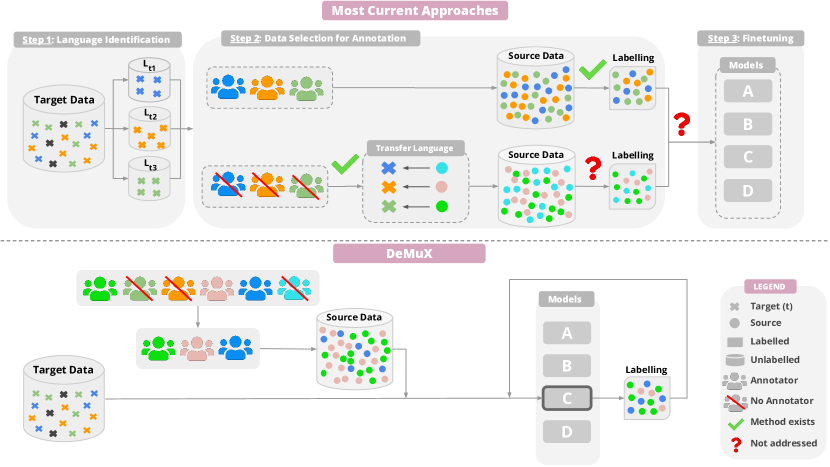
Figure 1: Top: Today, improving the performance of a model on multilingual target data is a three-step process. First, one would identify the target languages. Next, they would either collect data to label in these languages, or closely related transfer languages, based on annotator availability. Finally, they would fine-tune a model on the labelled data. However Step 1 excludes 98% of the world’s languages, Step 2 is constrained by annotators or linguistic feature information, and Step 3 of factoring in the model to fine-tune, largely remains unaccounted for. Bottom: With our end-to-end framework , we prescribe the exact data to label from a vast pool of multilingual source data, that provides for best transfer to the target, for a given model.

In this work, we aim to provide a solution to the above problem by introducing , an end-to-end framework that replaces the pipelined approach to multilingual data annotation (Figure 1). By directly selecting datapoints to annotate, bypasses several stages of the pipeline, that are barriers for most languages. The alleviation of needing to identify the target languages itself (Step 1: Figure 1), implies that it can be used for noisy, unidentifiable, or code-mixed targets.

makes decisions at the instance level by using information about the pre-trained multilingual language model’s (MultiLM’s) representation space. This ensures that the data annotation process is aware of the model ultimately being utilized. Concretely, we draw from the principles of active learning (AL) Cohn et al. (1996); Settles (2009) for guidance on model-aware criteria for point selection. AL aims to identify the most informative points (to a specific model) to label from a stream of unlabelled source data. Through iterations of model training, data acquisition and human annotation, the goal is to achieve satisfactory performance on a target test set, labelling only a small fraction of the data. Past works Chaudhary et al. (2019); Kumar et al. (2022); Moniz et al. (2022) have leveraged AL in the special case where the same language(s) constitute the source and target set (Step 2 (upper branch): Figure 1). However, none so far have considered the case of source and target languages having unknown degrees of overlap; a far more pervasive problem for real-world applications that commonly build classifiers on multi-domain data Dredze and Crammer (2008). From the AL lens, this is particularly challenging since conventional strategies of choosing the most uncertain samples Settles (2009), could pick distracting examples from very dissimilar language distributions Longpre et al. (2022). Our strategies are designed to deal with this distribution shift by leveraging small amounts of unlabelled data in target languages.

In the rest of the paper, we first describe three AL strategies based on the principles of a) semantic similarity with the target; b) uncertainty; and c) a combination of the two, which picks uncertain points in target points’ local neighborhood (§3). We experiment with tasks of varying complexity, categorized based on their label structure: token-level (NER and POS), sequence-level (NLI), and question answering (QA). We test our strategies in a zero-shot setting across three MultiLMs and five target language configurations, for a budget of 10,000 examples acquired in five AL rounds (§4).

We find that our strategies outperform previous baselines in most cases, including those with multilingual target sets. The extent varies, based on the budget, the task, the languages and models (§5). Overall, we observe that the hybrid strategy performs best for token-level tasks, but picking globally uncertain points gains precedence for NLI and QA. To test the applicability of in resource constrained settings, we experiment with lower budgets ranging from 5-1000 examples, acquired in a single AL round. In this setting, we observe gains of upto 8-11 F1 points for token-level tasks, and 2-5 F1 for complex tasks like NLI and QA. For NLI, our strategies surpass the gold standard of fine-tuning in target languages, while being zero-shot.

2 Notation

Assume that we have a set of source languages, ${L_{s}}=\{l^{1}_{s}\ldots l^{n}_{s}\}$, and a set of target languages, ${L_{t}}=\{l^{1}_{t}\ldots l^{m}_{t}\}$. ${L_{s}}$ and ${L_{t}}$ are assumed to have unknown degrees of overlap.

Further, let us denote the corpus of unlabelled source data as $\mathcal{X}_{s}=\{x^{1}_{s}\ldots x^{N}_{s}\}$ and the unlabelled target data as $\mathcal{X}_{t}=\{x^{1}_{t}\ldots x^{M}_{t}\}$.

Our objective is to label a total budget of ${B}$ data points over ${K}$ AL rounds from the source data. The points to select in each round can then be calculated by $b=\frac{B}{K}$. Thus considering the super-set $\mathcal{S}^{b}=\{\mathbf{X}\subset\mathcal{X}_{s}~{}\big{|}~{}\lvert\mathbf{X}\rvert=b\}$ of all $b$-sized subsets of $\mathcal{X}_{s}$, our objective is to select some $\mathbf{X}^{*}\in\mathcal{S}^{b}$ according to an appropriate criterion.

3 Annotation Strategies

Based on the broad categorizations of AL methods as defined by Zhang et al. (2022), we design three annotation strategies that are either representation-based, information-based, or hybrid. The first picks instances that capture the diversity of the dataset; the second picks the most uncertain points which are informative to learn a robust decision boundary; and the third focuses on optimally combining both criteria. In contrast to the standard AL setup, there are two added complexities in our framework: a) source-target domain mismatch; b) multiple distributions for each of our target languages. We therefore design our measures to select samples that are semantically similar (from the perspective of the MultiLM) to the target domain Longpre et al. (2022).

All strategies build upon reliable distance and uncertainty measures, whose implementation varies based on the type of task, i.e. whether the task is token-level, sequence-level or question answering. A detailed visualization of how these are calculated can be found in §A.1. Below, we formally describe the three strategies, also detailing the motivation behind our choices.

3.1 AVERAGE-DIST

AVERAGE-DIST constructs the set $\mathbf{X}^{*}$ such that it minimizes the average distance of points from $\mathcal{X}_{t}$ under an embedding function $f~{}:~{}\mathcal{X}\rightarrow\mathcal{R}^{d}$ defined by the MultiLM. This is a representation-based strategy that picks points lying close to the unlabelled target pool McCallum et al. (1998); Settles and Craven (2008). The source points chosen are informative since they are prototypical of the target data in the representation space (Figure 2(a)). Especially for low degrees of overlap between source and target data distributions, this criterion can ignore uninformative source points. Formally,

$$\mathbf{X}^{*}=\mathrm{argmin}_{~{}\mathbf{X}~{}\in~{}\mathcal{S}^{b}}~{}\sum_{x_{s}\in\mathbf{X}}d_{t}\left(x_{s}\right)$$

Where

$$d_{t}\left(x\right)=\frac{1}{\lvert\mathcal{X}_{t}\rvert}\sum_{x^{j}_{t}\in\mathcal{X}_{t}}\left\|f\left(x\right)-f\left(x^{j}_{t}\right)\right\|$$

For all task types, we use embeddings of tokens fed into the final classifier, to represent the whole sequence. For NLI and QA, this is the [CLS] token embedding. For token-level tasks, we compute the mean of the initial sub-word token embeddings for each word, as this is the input provided to the classifier to determine the word-level tag.

(a) AVERAGE-DIST

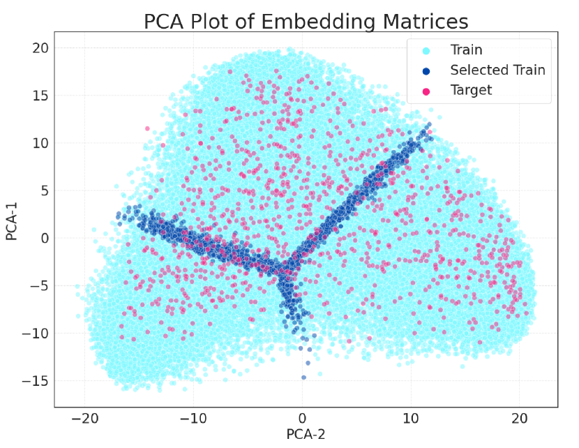
(b) UNCERTAINTY

(c) KNN-UNCERTAINTY

Figure 2: Visualization of datapoints selected using strategies detailed in Section 3, for a three-class sequence classification task (XNLI). AVERAGE-DIST selects points (dark blue) at a minimum average distance from the target (pink); UNCERTAINTY selects most uncertain points lying at the decision boundary of two classes, and KNN-UNCERTAINTY selects uncertain points in the target neighborhood.

3.2 UNCERTAINTY

Uncertainty sampling Lewis (1995) improves annotation efficiency by choosing points that the model would potentially misclassify in the current AL iteration. Uncertainty measures for each task-type can be found below:

Sequence-Level: We use margin-sampling Scheffer et al. (2001); Schein and Ungar (2007), which selects points having the least difference between the model’s probabilities for the top-two classes. We compute the output probability distribution for all unlabeled samples in $\mathcal{X}_{s}$ and select samples with the smallest margin. Formally,

$$\mathbf{X}^{*}=\mathrm{argmin}_{~{}\mathbf{X}~{}\in~{}\mathcal{S}^{b}}~{}\sum_{x_{s}\in\mathbf{X}}P_{\Delta}\left(x_{s}\right)$$

Where

$$P_{\Delta}\left(x\right)=p_{c_{1}}(x)-p_{c_{2}}(x)$$

$p_{c_{1}}(x)$ and $p_{c_{2}}(x)$ are the predicted probabilities of the top-two classes for an unlabeled sample $x$.

Token-level: For token-level tasks we first compute the margin (as described above) for each token in the sequence. Then, we assign the minimum margin across all tokens as the sequence margin score and choose construct $\mathbf{X}^{*}$ with sequences having the least score. Formally,

$$\mathbf{X}^{*}=\mathrm{argmin}_{~{}\mathbf{X}~{}\in~{}\mathcal{S}^{b}}~{}\sum_{x_{s}\in\mathbf{X}}\texttt{MARGIN-MIN}\left(x_{s}\right)$$

Where

$$\texttt{MARGIN-MIN}\left(x\right)=\min_{i=1}^{\lvert x\rvert}\left(p^{i}_{c_{1}}(x)-p^{i}_{c_{2}}(x)\right)$$

Question Answering: The QA task we investigate involves extracting the answer span from a relevant context for a given question. This is achieved by selecting tokens with the highest start and end probabilities as the boundaries, and predicting tokens within this range as the answer. Hence, samples having the lowest start and end probabilities, qualify as most uncertain. Formally,

$$\mathbf{X}^{*}=\mathrm{argmin}_{~{}\mathbf{X}~{}\in~{}\mathcal{S}^{b}}~{}\sum_{x_{s}\in\mathbf{X}}\texttt{SUM-PROB}\left(x_{s}\right)$$

Where

$$\texttt{SUM-PROB}\left(x\right)=\max_{i=1}^{\lvert x\rvert}\log p^{i}_{s}(x){+}\max_{i=1}^{\lvert x\rvert}\log p^{i}_{e}(x)$$

Above, $\lvert x\rvert$ denotes the sequence length of the unlabeled sample $x$, and $p^{i}_{s}(x)$ and $p^{i}_{e}(x)$ represent the predicted probabilities for the start and end index, respectively.

Task Type	Task	Dataset	Languages (two-letter ISO code)
Token-level	Part-of-Speech Tagging (POS)	Universal Dependencies v2.5 Nivre et al. (2020)	tl, af, ru, nl, it, de, es, bg, pt, fr, te, et, el, fi, hu, mr, kk, hi, tr, eu, id, fa, ur, he, ar, ta, vi, ko, th, zh, yo, ja
	Named Entity Recognition (NER)	WikiAnn Rahimi et al. (2019)	nl, pt, bg, it, fr, hu, es, el, vi, fi, et, af, bn, de, tr, tl, hi, ka, sw, ru, mr, ml, jv, fa, eu, ko, ta, ms, he, ur, kk, te, my, ar, id, yo, zh, ja, th
Sequence-Level	Natural Language Inference (NLI)	XNLI Conneau et al. (2018)	es, bg, de, fr, el, vi, ru, zh, tr, th, ar, hi, ur, sw
Question Answering (QA)		TyDiQA Clark et al. (2020)	id, fi, te, ar, ru, sw, bn, ko

Table 1: Tasks and Datastes: is applied across tasks of varying complexity, as elucidated in Q1: §4.

3.3 KNN-UNCERTAINTY

As standalone measures, both distance and uncertainty based criteria have shortcomings. When there is little overlap between source and target, choosing source points based on UNCERTAINTY alone leads to selecting data that are uninformative to the target. When there is high degrees of overlap between source and target, the AVERAGE-DIST metric tends to produce a highly concentrated set of points (Figure 2(a)) – even if the model is accurate in that region of representation space – resulting in minimal coverage on the target set.

To design a strategy that combines the strengths of both distance and uncertainty, we first measure how well a target point’s uncertainty correlates with its neighborhood. We calculate the Pearson’s correlation coefficient ($\rho$) Pearson (1903) between the uncertainty of a target point in $\mathcal{X}_{t}$ and the average uncertainty of its top-$k$ neighbors in $\mathcal{X}_{s}$. We observe a statistically significant $\rho$ value > 0.7, for all tasks. A natural conclusion drawn from this is that decreasing the uncertainty of a target point’s neighborhood would decrease the uncertainty of the target point itself. Hence, we first select the top-$k$ neighbors for each $x_{t}\in\mathcal{X}_{t}$. Next, we choose the most uncertain points from these neighbors until we reach $b$ data points. Formally, until $\lvert\mathbf{X}^{*}\rvert=b$ :

$$\mathbf{X}^{*}=\mathrm{argmax}_{\{\mathbf{X}~{}\subset~{}\mathcal{N}_{t}^{k}~{}\big{|}~{}\lvert\mathbf{X}\rvert~{}=~{}b\}}\sum_{x_{s}~{}\in~{}\mathbf{X}}U(x_{s})$$

Where

$$\mathcal{N}_{t}^{k}=\bigcup_{j=1}^{|\mathcal{X}_{t}|}~{}\texttt{k-NEARESTNEIGHBORS}(x^{j}_{t},\mathcal{X}_{s})$$

Above, $U(x_{s})$ represents the uncertainty of the source point as calculated in §3.2.

4 Experimental Setup

Dataset	Single Target			Multi-Target
	HP	MP	LP	Geo	LPP
UDPOS	French	Turkish	Urdu	Telugu, Marathi, Urdu	Arabic, Hebrew, Japanese, Korean, Chinese, Persian, Tamil, Vietnamese, Urdu
NER	French	Turkish	Urdu	Indonesian, Malay, Vietnamese	Arabic, Indonesian, Malay, Hebrew, Japanese, Kazakh, Malay, Tamil, Telugu, Thai, Yoruba, Chinese, Urdu
XNLI	French	Turkish	Urdu	Bulgarian, Greek, Turkish	Arabic, Thai, Swahili, Urdu, Hindi
TyDiQA	Finnish	Arabic	Bengali	Bengali, Telugu	Swahili, Bengali, Korean

Table 2: Target language configurations. We run five experiments for each model and task, with the language sets above as targets (details in §4.2). All languages mentioned in Table 1 make up the source set, except the chosen target languages for a particular configuration.

Our setup design aims to address the following:

Q1) Does benefit tasks with varying complexity? Which strategies work well across different task types? (§4.1)
Q2) How well does perform across a varied set of target languages? Can it benefit multilingual target pools as well? (§4.2)
Q3) How do the benefits of vary across different MultiLMs? (§4.3)

4.1 Task and Dataset Selection

We have three distinct task types, based on the label format. We remove duplicates from each dataset to prevent selecting multiple copies of the same instance. Dataset details can be found in Table 1.

4.2 Source and Target Language Selection

We experiment with the zero-shot case of disjoint source and target languages, i.e., the unlabelled source pool contains no data from target languages. The train and validation splits constitute the unlabelled source or target data, respectively. Evaluation is done on the test split for each target language. With Q2) in mind, we experiment with five target settings (Table 2):

Single-target: We partition languages into three equal tiers based on zero-shot performance post fine-tuning on English: high-performing (HP), mid-performing (MP) and low-performing (LP), and choose one language from each, guided by two factors. First, we select languages that are common across multiple datasets, to study how data selection for the same language varies across tasks. From these, we choose languages that have similarities with the source set across different linguistic dimensions (obtained using lang2vec Littell et al. (2017)), to study the role of typological similarity for different tasks.

Multi-target: Here, we envision two scenarios:

Geo: Mid-to-low performing languages in geographical proximity are chosen. From an application perspective, this would allow one to improve a MultiLM for an entire geographical area.

LPP: All low-performing languages are pooled, to test whether we can collectively enhance the MultiLM’s performance across all of them.

4.3 Model Selection

We test across multiple MultiLMs: XLM-R Conneau et al. (2019), InfoXLM Chi et al. (2020), and RemBERT Chung et al. (2020). All models have a similar number of parameters ($\sim$550M-600M), and support 100+ languages. XLM-R is trained on monolingual corpora from CC-100 Conneau et al. (2019), InfoXLM is trained to maximize mutual information between multilingual texts, and RemBERT is a deeper model, that reallocates input embedding parameters to the Transformer layers.

4.4 Baselines

We include a number of baselines to compare our strategies against:

1) RANDOM: In each round, a random subset of $b$ data points from $\mathcal{X}_{s}$ is selected.

2) EGALITARIAN: An equal number of randomly selected data points from the unlabeled pool for each language, i.e. $|x_{s}|=b/|L_{s}|$; $\forall x_{s}\in\mathcal{X}_{s}$ is chosen. Debnath et al. (2021) demonstrate that this outperforms a diverse set of alternatives.

3) LITMUS: LITMUS Srinivasan et al. (2022) is a tool to make performance projections for a fine-tuned model, but can also be used to generate data labeling plans, based on the predictor’s projections. We only run this for XLM-R since the tool requires past fine-tuning performance profiles, and XLM-R is supported by default.

4) GOLD: This involves training on data from the target languages itself. Given all other strategies are zero-shot, we expect GOLD to out-perform them and help determine an upper bound on performance.

4.5 Fine-tuning Details

We first fine-tune all MultiLMs on English (EN-FT) and continue fine-tuning on data selected using , similar to Lauscher et al. (2020); Kumar et al. (2022). We experiment with a budget of 10,000 examples acquired in five AL rounds, except for TyDiQA, where our budget is 5,000 examples (TyDiQA is of the order of 35-40k samples overall across ten languages, and this is to ensure fair comparison with our gold strategy). For each model, we first obtain EN-FT and continually fine-tune using . Hyperparameter details are given in §A.3, and all results are averaged across three seeds: 2, 22, 42. We fine-tune using a fixed number of epochs without early stopping, given the lack of a validation set in our setup (we assume no labelled target data).

5 Results

How does perform overall? We present results for NER, POS, NLI and QA in Tables 3, 4, 5 and 6, respectively. In summary, the best-performing strategies outperform the best performing baselines in 84% of the cases, with variable gains dependant on the task, model and target languages. In the remaining cases, the drop is within 1% absolute delta from the best-performing baseline.

How does fare on multilingual target pools? We observe consistent gains given multilingual target pools as well (Geo and LPP). We believe this is enabled by the language-independent design of our strategies, which makes annotation decisions at a per-instance level. This has important consequences, since this would enable researchers, like those at Company Y, to better models for all the languages that they care about.

Does the model select data from the same languages across tasks? No! We find that selected data distributions vary across tasks for the same target languages. For example, when the target language is Urdu, chooses 70-80% of samples from Hindi for NLI and POS, but prioritizes Farsi and Arabic (35-45%) for NER. Despite Hindi and Urdu’s syntactic, genetic, and phonological similarities as per lang2vec, their differing scripts underscore the significance of script similarity in NER transfer. This also proves that analysing data selected by can offer linguistic insights into the learned task-specific representations.

	Method	HP	MP	LP	Geo	LPP
XLM-R	EN-FT	80.0	79.5	65.6	61.0	45.8
	GOLD	90.1	92.8	94.5	81.2	73.7
	BASEegal	85.4	87.6	84.0	80.6	62.8
	$\method_{knn}$	87.8	89.2	85.8	82.4	62.3
	$\Delta_{base}$	2.4	1.6	1.8	1.8	-0.5
InfoXLM	EN-FT	80.5	82.8	65.4	64.2	44.8
	GOLD	90.0	92.8	94.6	83.5	74.9
	BASEegal	84.0	87.6	83.2	80.9	63.4
	$\method_{knn}$	87.4	89.2	85.5	82.2	64.2
	$\Delta_{base}$	3.4	1.6	2.2	1.3	0.8
RemBERT	EN-FT	78.8	80.2	55.7	61.1	48.4
	GOLD	89.4	92.1	93.5	79.8	70.1
	BASEegal	84.6	86.8	82.3	79.2	59.8
	$\method_{knn}$	87.1	89.0	85.7	79.8	62.1
	$\Delta_{base}$	2.5	2.2	3.4	0.6	2.3

Table 3: PAN-X Results (F1): We observe gains across all models and KNN-UNCERTAINTY performs best. $\Delta_{base}$ represents the delta from baseline.

	Method	HP	MP	LP	Geo	LPP
XLM-R	EN-FT	81.7	75.5	71.5	80.2	62.2
	GOLD	95.6	81.2	93.2	91.8	88.2
	BASEegal	87.1	79.6	88.4	85.7	68.9
	$\method_{knn}$	87.5	80.1	90.1	86.1	70.9
	$\Delta_{base}$	0.4	0.5	1.7	0.4	2.0
InfoXLM	EN-FT	79.6	74.0	59.0	73.6	58.2
	GOLD	95.7	81.4	93.3	92.0	88.7
	BASEegal	88.0	79.4	88.8	86.3	67.8
	$\method_{knn}$	87.8	79.5	90.4	86.0	66.8
	$\Delta_{base}$	-0.3	0.1	1.6	-0.3	-1.0
RemBERT	EN-FT	72.9	71.1	50.6	66.1	55.7
	GOLD	95.1	80.8	92.3	91.2	86.8
	BASEegal	86.9	78.1	85.8	83.8	67.8
	$\method_{knn}$	87.4	77.7	88.2	84.2	68.0
	$\Delta_{base}$	0.5	-0.3	2.4	0.4	0.2

Table 4: UDPOS Results (F1): We observe modest gains for a 10k budget, but higher gains for lower budgets (§6)

.

	Method	HP	MP	LP	Geo	LPP
XLM-R	EN-FT	81.8	77.3	69.9	80.1	73.4
	GOLD	81.6	79.5	70.3	81.6	76.0
	BASEegal	81.6	78.8	73.0	80.9	75.6
	$\method_{avg}$	83.7	79.9	75.3	82.2	77.1
	$\Delta_{base}$	2.1	1.1	2.3	1.3	1.5
	$\Delta_{gold}$	2.1	0.4	5.0	0.6	1.1
InfoXLM	EN-FT	81.9	77.3	68.8	79.8	71.5
	GOLD	83.6	80.6	73.7	82.4	77.7
	BASEegal	83.7	79.8	74.6	81.5	77.3
	$\method_{avg}$	84.8	80.8	75.9	83.1	77.8
	$\Delta_{base}$	1.1	1.0	1.3	1.6	0.5
	$\Delta_{gold}$	1.2	0.2	2.2	0.7	0.1
RemBERT	EN-FT	83.1	73.9	52.5	77.8	63.0
	GOLD	81.1	73.3	63.1	76.0	67.5
	BASEegal	80.0	75.3	63.9	76.4	67.9
	$\method_{avg}$	81.7	76.1	67.6	78.6	70.9
	$\Delta_{base}$	1.7	0.8	3.7	2.2	3.0
	$\Delta_{gold}$	0.6	2.8	4.5	2.6	3.4

Table 5: XNLI Results (F1): Here we even surpass the gold standard of in-language finetuning. Details in §5.

	Method	HP	MP	LP	Geo	LPP
XLM-R	EN-FT	78.9	73.2	79.9	80.7	78.5
	GOLD	81.2	83.8	83.7	84.7	81.0
	BASEegal	79.9	81.7	79.6	81.1	78.7
	$\method_{unc}$	80.8	82.9	80.3	81.0	77.8
	$\Delta_{base}$	0.9	1.2	0.7	-0.1	-0.9
InfoXLM	EN-FT	77.6	75.4	82.2	81.9	78.8
	GOLD	80.7	85.0	86.3	87.1	81.1
	BASEegal	80.5	82.3	82.2	82.3	78.1
	$\method_{unc}$	81.8	84.1	80.8	82.6	77.8
	$\Delta_{base}$	1.3	1.8	-1.4	0.3	-0.3
RemBERT	EN-FT	79.7	73.0	82.9	78.0	78.2
	GOLD	78.4	80.1	86.7	84.4	80.5
	BASEegal	81.3	78.9	82.8	76.5	75.3
	$\method_{unc}$	82.7	80.2	80.6	78.0	76.1
	$\Delta_{base}$	1.4	1.3	-2.2	1.5	0.8

Table 6: TyDiQA Results (F1): UNCERTAINTY works best here. Despite TyDiQA being composed of typologically diverse languages and being extremely small (35-40k samples), we observe modest gains across multiple configs.

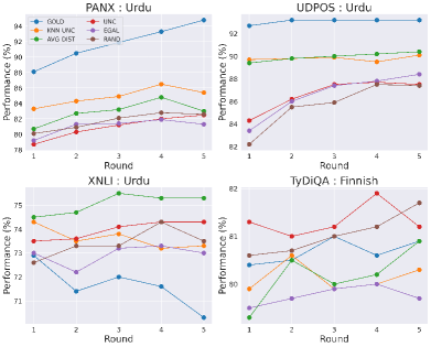
Figure 3: Performance across different AL rounds for XLM-R: Semantic similarity with target matters most for token-level tasks, but uncertainty gains importance for NLI and QA. (AVG-DIST picks maximally uncertain points for NLI due to the nature of the dataset (§5).

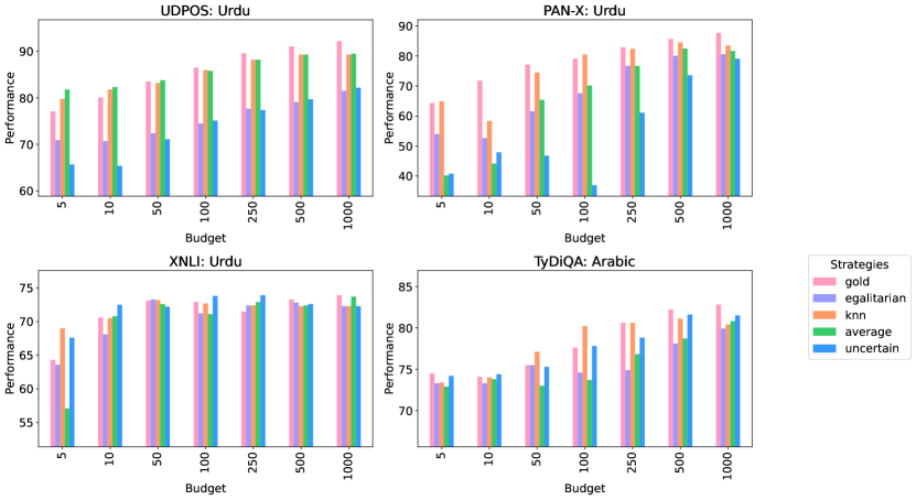
Figure 4: Multiple budgets, one AL round: We experiment with low-budgets acquired using the EN-FT model. We observe gains of up to 8-11 F1 over baselines for 5-100 examples, with a trend of diminishing gains given larger budgets. All runs averaged across three seeds (2, 22, 42).

Which strategies work well across different task types? Our hybrid strategy, which picks uncertain points in the local neighborhood of target points, performs best for token-level tasks, whereas globally uncertain points maximize performance for NLI and QA. For NLI, both AVERAGE-DIST and UNCERTAINTY outperform baselines, the former proving more effective. On further analysis, we find that this is an artifact of the the nature of the dataset which is balanced across three labels, and is strictly parallel. This makes AVERAGE-DIST select high-uncertainty points at decision boundaries’ centroid, as visualized in Figure 2(a). Our finding of different strategies working well for different tasks is consistent with past works. For example, Settles and Craven (2008) find information density (identifying semantically similar examples), to work best for sequence-labeling tasks; Marti Roman (2022) discuss how uncertainty-based methods perform best for QA; and Kumar et al. (2022) also recommend task-dependant labeling strategies. By including multiple tasks and testing multiple strategies for each, we provide guidance to everyday practitioners on the best strategy, given a task.

How does performance vary across models? For all models, the EN-FT performance is similar, except for UDPOS, where XLM-R is consistently better than InfoXLM and RemBERT. We see this play a role in the consistent gains provided by across languages for XLM-R, as opposed to RemBERT and InfoXLM. We hypothesize that the better a model’s representations, the better our measures of distance and uncertainty, which inherently improves data selection.

6 Further Analysis

What is the minimum budget for which we can observe gains in one AL round? To deploy in resource-constrained settings, we test its applicability in low-budget settings, ranging from 5,10,50,100,250,500,1000, acquired using the EN-FT model only. As shown in Figure 4, we observe gains across all budget levels. Notably, we observe gains of up to 8-11 F1 points for token-level tasks, and 2-5 F1 points for NLI and QA, for most lower budgets (5-100 examples). These gains diminish as the budget increases. For complex tasks like NLI and QA, semantic similarity with the target holds importance when the budgets is below 500 examples, but picking globally uncertain points gains precedence for larger budgets.

Do the selected datapoints matter or does following the language distribution suffice? not only identifies transfer languages but also selects specific data for labeling. To evaluate its importance, we establish the language distribution of data selected using and randomly select datapoints following this distribution. Despite maintaining this distribution, performance still declines (§A.4), indicating that precise datapoint selection in identified transfer languages is vital.

7 Related Work

Multilingual Fine-tuning: Traditionally models were fine-tuned on English, given the availability of labeled data across all tasks. However, significant transfer gaps were observed across languages Hu et al. (2020) leading to the emergence of two research directions. The first emphasizes the significance of using few-shot target language data Lauscher et al. (2020) and the development of strategies for optimal few-shot selection Kumar et al. (2022); Moniz et al. (2022). The second focuses on choosing the best source languages for a target, based on linguistic features Lin et al. (2019) or past model performances Srinivasan et al. (2022). Discerning a globally optimal transfer language however, has been largely ambiguous Pelloni et al. (2022) and the language providing for highest empirical transfer is at times inexplicable by known linguistic relatedness criteria Pelloni et al. (2022); Turc et al. (2021). By making decisions at a data-instance level rather than a language level, removes the reliance on linguistic features and sidesteps ambiguous consensus on how MultiLMs learn cross-lingual relations, while prescribing domain-relevant instances to label.

Active learning for NLP: AL has seen wide adoption in NLP, being applied to tasks like text classification Karlos et al. (2012); Li et al. (2013), named entity recognition Shen et al. (2017); Wei et al. (2019); Erdmann et al. (2019), and machine translation Miura et al. (2016); Zhao et al. (2020), among others. In the multilingual context, past works Moniz et al. (2022); Kumar et al. (2022); Chaudhary et al. (2019) have applied AL to selectively label data in target languages. However, they do not consider cases with unknown overlap between source and target languages. This situation, similar to a multi-domain AL setting, is challenging as data selection from the source languages may not prove beneficial for the target Longpre et al. (2022).

8 Conclusion

In this work, we introduce , an end-to-end framework that selects data to label from vast pools of unlabelled multilingual data, under an annotation budget. ’s design is language-agnostic, making it viable for cases where source and target data do not overlap. We design three strategies drawing from AL principles that encompass semantic similarity with the target, uncertainty, and a hybrid combination of the two. Our strategies outperform strong baselines for 84% of target language configurations (including multilingual target sets) in the zero-shot case of disjoint source and target languages, across three models and four tasks: NER, UDPOS, NLI and QA. We find that semantic similarity with the target mostly benefits token-level tasks, while picking uncertain points gains precedence for complex tasks like NLI and QA. We further analyse ’s applicability in low-budget settings and observe gains of up to 8-11 F1 points for some tasks, with a trend of diminishing gains for larger budgets. We hope that our work helps improve the capabilities of MultiLMs for desired languages, in a cost-efficient way.

9 Limitations

With ’s wider applicability across languages come a few limitations as we detail below:

Inference on source data: relies on model representations and its output ditribution for each example. This requires us to run inference on all of the source data; which can be time-consuming. However, one can run parallel CPU-inference which greatly reduces latency.

Aprior Model Selection: We require knowing the model apriori which might mean a different labeling scheme for different models. This a trade-off we choose in pursuit of better performance for the chosen model, but it may not be the most feasible solution for all users.

Refinement to the hybrid approach: Our hybrid strategy picks the most uncertain points in the neighborhood of the target. However, its current design prioritizes semantic similarity with the target over global uncertainty, since we first pick top-$k$ neighbors and prune this set based on uncertainty. However, it will be interesting to experiment with choosing globally uncertain points first and then pruning the set based on target similarity. For NLI and QA, we observe that globally uncertain points help for higher budgets but choosing nearest neighbors helps most for lower budgets. Therefore, this alternative may work better for these tasks, and is something we look to explore in future work.

10 Acknowledgements

We thanks members of the Neulab and COMEDY, for their invaluable feedback on a draft of this paper. This work was supported in part by grants from the National Science Foundation (No. 2040926), Google, Two Sigma, Defence Science and Technology Agency (DSTA) Singapore, and DSO National Laboratories Singapore.

Appendix A Appendix

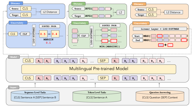
Figure 5: An overview of how distance and uncertainty are measured in our setup. $A_{1},A_{2},A_{3}$ denote three words in Sentence A that are tokenized into 2, 3, and 1 subword, respectively.

A.1 Distance and Uncertainty Measurements

All of our strategies our based on reliable distance and uncertainty measures. Once these are established, it is easy to extend to other tasks and models. An overview of how these are measured for the tasks in our study can be found in Figure 5. These are formally described in the paper, in Section 3.

A.2 Uncertainty Details

For token-level tasks, we investigate two strategies. First, we employ the Mean Normalized Log Probability (MNLP) Shen et al. (2017) method, which has been demonstrated as an effective uncertainty measure for Named Entity Recognition (NER). This approach selects instances for which the log probability of model prediction, normalized by sequence length, is the lowest. Formally,

$$\mathbf{X}^{*}=\mathrm{argmin}_{~{}\mathbf{X}~{}\in~{}\mathcal{S}^{b}}~{}\sum_{x_{s}\in\mathbf{X}}\texttt{MNLP}\left(x_{s}\right)$$

Where

$$\texttt{MNLP}\left(x\right)=\frac{1}{\lvert x\rvert}\sum_{i=1}^{\lvert x\rvert}\log p^{i}_{c_{1}}(x)$$

In this equation, $\lvert x\rvert$ denotes the sequence length of the unlabeled sample $x$, and $p^{i}_{c_{1}}(x)$ represents the predicted probability of the most probable class for the $i^{th}$ token in the sequence.

Concurrently, we also explore margin-based uncertainty techniques (MARGIN-MIN). For each token in the sequence, we compute the margin as the difference between the probabilities of the top two classes. Then, we assign the minimum margin across all tokens as the sequence margin score and choose sequences with the smallest margin score. Formally,

$$\mathbf{X}^{*}=\mathrm{argmin}_{~{}\mathbf{X}~{}\in~{}\mathcal{S}^{b}}~{}\sum_{x_{s}\in\mathbf{X}}\texttt{MARGIN-MIN}\left(x_{s}\right)$$

Where

$$\texttt{MARGIN-MIN}\left(x\right)=\min_{i=1}^{\lvert x\rvert}\left(p^{i}_{c_{1}}(x)-p^{i}_{c_{2}}(x)\right)$$

We eventually choose the margin based technique given better performance for both token level tasks.

Dataset	Single Target			Multi-Target
	HP	MP	LP	Geo	LP Pool
UDPOS	fr:4938	tr:984	ur:545	te:130, mr:46, ur:545	ar:906, he:484, ja:511, ko:3014, zh:2689, fa:590, ta:80, vi:794, ur:545
NER	fr:9300	tr:9497	ur:944	id:7525, my:100, vi:8577	ar:9319,id:7525, my:100, he:9538, ja:9641, kk:910, ms:761, ta:965, te:939, th:9293, yo:93, zh:9406, ur:944
XNLI	fr:2490	tr:2490	ur:2490	bg:2490, el:2490, tr:2490	ar:2490, th:2490 ,sw:2490, ur:2490, hi:2490
TyDiQA	fi:1371	ar:2961	bn:478	bn:478, te:1113	sw:551, bn:478, ko:325

Table 7: Number of unlabelled target examples used in each configuration. This is the size of the validation set.

Model	Dataset	LR	Epochs
XLM-R	NER	2e-5	10
	UDPOS	2e-5	10
	XNLI	5e-6	10
	TyDiQA	1e-5	3
InfoXLM	NER	2e-5	10
	UDPOS	2e-5	10
	XNLI	5e-6	10
	TyDiQA	1e-5	3
RemBERT	NER	8e-6	10
	UDPOS	8e-6	10
	XNLI	8e-6	10
	TyDiQA	1e-5	3

Table 8: Hyperparameter Details.

Dataset	Single Target			Multi-Target
	HP	MP	LP	Geo	LP Pool
UDPOS	fr	tr	ur	te, mr, ur	ar, he, ja, ko, zh, fa, ta, vi, ur
	it: 3434	et:799, fa:598, ja:890, vi:694	de:5095, eu:84, hi:3323, mr:92, nl:556	ar:93, bg:68, et:3197,eu:84, fr:65, hi:3323, ja:890	hi:830
NER	fr	tr	ur	id, my, vi	ar, id, my, he, ja, kk, ms, ta, te, th, yo, zh, ur
	it: 572	he: 4582; mr: 1015, nl: 4393	fa: 4007, ms: 79, ta: 788, vi: 62	bn:1000, he:572, ko:469, ms:79	bn:62, ko:4699, ml:4306
XNLI	fr	tr	ur	bg, el, tr	ar, th, sw, ur, hi
	ur:781, zh:6250	ru:781, ur:6250	hi:6250	ru:781, ur:6250	bg:6250, de:781, fr:781, vi:781
TyDiQA	fi	ar	bn	bn, te	sw, bn, ko
	ar:185, bn:119, id:142, ko:2, ru:1, sw:17, te:4450	bn:14, fi:2742, ko:20, sw:4, te:2	ar:740	ar:46, fi:2742, id:570, ko:325, ru:5, sw:8	-

Table 9: LITMUS prescribed annotation budget: LITMUS prescribes how many samples to select from each language. We select a random sample of data following the prescribed annotation.

A.3 Fine-tuning Details

As mentioned in the text, we first fine-tune each model on EN using the hyperparameters mentioned in the paper. Hyperparameters are in Table 8 and we report average results across three seeds: 2, 22, 42. For UDPOS, we include all languages except Tagalog, Thai, Yoruba and Kazakh, because they do not have training data for the task.

A.4 Detailed Results

The detailed results for the first ablation study where we test for multiple budgets in one AL round, can be found in Table 11. Results for the second ablation, where we fine-tune models on randomly selected data that follows the same language distribution as , can be found in Table 10.

Dataset	Strategy	AL Round
		1	2	3	4	5
PAN-X	SR	81.1	81.9	84.1	85.1	84.0
		83.2	83.1	84.1	85.8	85.2
	$\Delta$	2.0	1.2	0.0	0.7	1.2
UDPOS	SR	89.9	89.3	89.5	90.0	89.8
		89.7	89.8	89.9	89.5	90.1
	$\Delta$	-0.2	0.5	0.5	-0.4	0.3
XNLI	SR	73.3	73.8	73.8	73.8	73.9
		74.5	74.7	75.5	75.3	75.3
	$\Delta$	1.2	0.9	1.6	1.5	1.4
TyDiQA	SR	80.6	81.5	81.5	82.0	81.7
		82.8	83.2	83.2	83.5	83.8
	$\Delta$	2.2	1.7	1.8	1.5	2.1

Table 10: Detailed results: SR stands for SAME-RATIO. Same data distribution across languages but a random subset of datapoints selected.

Dataset	Budget	Strategy
UDPOS		GOLD	EGAL	KNN-UNC	AVG-DIST	UNC
	5	77.1	70.9	79.8	81.8	65.7
	10	80.1	70.7	81.8	82.3	65.4
	50	83.5	72.4	83.2	83.8	71.1
	100	86.5	74.5	86.0	85.8	75.1
	250	89.6	77.7	88.2	88.2	77.4
	500	91.1	79.1	89.3	89.3	79.7
	1000	92.2	81.5	89.3	89.5	82.2
PAN-X	5	64.3	54	64.9	40.2	40.8
	10	71.8	52.7	58.4	44.2	47.9
	50	77.1	61.6	74.5	65.4	46.8
	100	79.2	67.6	80.5	70.2	37
	250	82.9	76.7	82.4	76.7	61.1
	500	85.7	80.1	84.5	82.5	73.6
	1000	87.7	80.6	83.5	81.7	79.1
XNLI	5	64.3	63.6	69	57.1	67.6
	10	70.6	68.1	70.5	70.8	72.5
	50	73.1	73.3	73.2	72.6	72.2
	100	72.9	71.2	72.7	71.1	73.8
	250	71.5	72.4	72.4	72.9	73.9
	500	73.3	72.8	72.3	72.4	72.6
	1000	73.9	72.3	72.3	73.7	72.3
TyDiQA	74.5	73.3	73.4	72.9	74.2	74.2
	74.1	73.3	74.0	73.8	74.4	74.4
	75.5	75.5	77.1	73.0	75.3	75.3
	77.6	74.6	80.2	73.7	77.8	77.8
	80.6	74.9	80.6	76.8	78.8	78.8
	82.2	78.1	81.1	78.7	81.6	81.6
	82.8	79.9	80.4	80.8	81.5	81.5

Table 11: Detailed results: Multiple budgets, one AL round

References

- Chaudhary et al. (2019) Aditi Chaudhary, Jiateng Xie, Zaid Sheikh, Graham Neubig, and Jaime G Carbonell. 2019. A little annotation does a lot of good: A study in bootstrapping low-resource named entity recognizers. arXiv preprint arXiv:1908.08983.
- Chi et al. (2020) Zewen Chi, Li Dong, Furu Wei, Nan Yang, Saksham Singhal, Wenhui Wang, Xia Song, Xian-Ling Mao, Heyan Huang, and Ming Zhou. 2020. Infoxlm: An information-theoretic framework for cross-lingual language model pre-training. arXiv preprint arXiv:2007.07834.
- Chung et al. (2020) Hyung Won Chung, Thibault Fevry, Henry Tsai, Melvin Johnson, and Sebastian Ruder. 2020. Rethinking embedding coupling in pre-trained language models. arXiv preprint arXiv:2010.12821.
- Clark et al. (2020) Jonathan H Clark, Eunsol Choi, Michael Collins, Dan Garrette, Tom Kwiatkowski, Vitaly Nikolaev, and Jennimaria Palomaki. 2020. Tydi qa: A benchmark for information-seeking question answering in typologically diverse languages. Transactions of the Association for Computational Linguistics, 8:454–470.
- Cohn et al. (1996) David A Cohn, Zoubin Ghahramani, and Michael I Jordan. 1996. Active learning with statistical models. Journal of artificial intelligence research, 4:129–145.
- Conneau et al. (2019) Alexis Conneau, Kartikay Khandelwal, Naman Goyal, Vishrav Chaudhary, Guillaume Wenzek, Francisco Guzmán, Edouard Grave, Myle Ott, Luke Zettlemoyer, and Veselin Stoyanov. 2019. Unsupervised cross-lingual representation learning at scale. arXiv preprint arXiv:1911.02116.
- Conneau et al. (2018) Alexis Conneau, Guillaume Lample, Ruty Rinott, Adina Williams, Samuel R Bowman, Holger Schwenk, and Veselin Stoyanov. 2018. Xnli: Evaluating cross-lingual sentence representations. arXiv preprint arXiv:1809.05053.
- Debnath et al. (2021) Arnab Debnath, Navid Rajabi, Fardina Fathmiul Alam, and Antonios Anastasopoulos. 2021. Towards more equitable question answering systems: How much more data do you need? arXiv preprint arXiv:2105.14115.
- Dredze and Crammer (2008) Mark Dredze and Koby Crammer. 2008. Online methods for multi-domain learning and adaptation. In Proceedings of the 2008 Conference on Empirical Methods in Natural Language Processing, pages 689–697.
- Erdmann et al. (2019) Alexander Erdmann, David Joseph Wrisley, Christopher Brown, Sophie Cohen-Bodénès, Micha Elsner, Yukun Feng, Brian Joseph, Béatrice Joyeux-Prunel, and Marie-Catherine de Marneffe. 2019. Practical, efficient, and customizable active learning for named entity recognition in the digital humanities. Association for Computational Linguistics.
- Hu et al. (2020) Junjie Hu, Sebastian Ruder, Aditya Siddhant, Graham Neubig, Orhan Firat, and Melvin Johnson. 2020. Xtreme: A massively multilingual multi-task benchmark for evaluating cross-lingual generalisation. In International Conference on Machine Learning, pages 4411–4421. PMLR.
- Karlos et al. (2012) Stamatis Karlos, Nikos Fazakis, Sotiris Kotsiantis, and Kyriakos Sgarbas. 2012. An empirical study of active learning for text classification. Advances in Smart Systems Research, 6(2):1.
- Kumar et al. (2022) Shanu Kumar, Sandipan Dandapat, and Monojit Choudhury. 2022. " diversity and uncertainty in moderation" are the key to data selection for multilingual few-shot transfer. arXiv preprint arXiv:2206.15010.
- Lauscher et al. (2020) Anne Lauscher, Vinit Ravishankar, Ivan Vulić, and Goran Glavaš. 2020. From zero to hero: On the limitations of zero-shot cross-lingual transfer with multilingual transformers. arXiv preprint arXiv:2005.00633.
- Lewis (1995) David D Lewis. 1995. A sequential algorithm for training text classifiers: Corrigendum and additional data. In Acm Sigir Forum, volume 29, pages 13–19. ACM New York, NY, USA.
- Li et al. (2013) Shoushan Li, Yunxia Xue, Zhongqing Wang, and Guodong Zhou. 2013. Active learning for cross-domain sentiment classification. In Twenty-Third International Joint Conference on Artificial Intelligence. Citeseer.
- Lin et al. (2019) Yu-Hsiang Lin, Chian-Yu Chen, Jean Lee, Zirui Li, Yuyan Zhang, Mengzhou Xia, Shruti Rijhwani, Junxian He, Zhisong Zhang, Xuezhe Ma, et al. 2019. Choosing transfer languages for cross-lingual learning. arXiv preprint arXiv:1905.12688.
- Littell et al. (2017) Patrick Littell, David R Mortensen, Ke Lin, Katherine Kairis, Carlisle Turner, and Lori Levin. 2017. Uriel and lang2vec: Representing languages as typological, geographical, and phylogenetic vectors. In Proceedings of the 15th Conference of the European Chapter of the Association for Computational Linguistics: Volume 2, Short Papers, volume 2, pages 8–14.
- Longpre et al. (2022) Shayne Longpre, Julia Reisler, Edward Greg Huang, Yi Lu, Andrew Frank, Nikhil Ramesh, and Chris DuBois. 2022. Active learning over multiple domains in natural language tasks. arXiv preprint arXiv:2202.00254.
- Marti Roman (2022) Salvador Marti Roman. 2022. Active learning for extractive question answering.
- McCallum et al. (1998) Andrew McCallum, Kamal Nigam, et al. 1998. Employing em and pool-based active learning for text classification. In ICML, volume 98, pages 350–358. Citeseer.
- Miura et al. (2016) Akiva Miura, Graham Neubig, Michael Paul, and Satoshi Nakamura. 2016. Selecting syntactic, non-redundant segments in active learning for machine translation. In Proceedings of the 2016 Conference of the North American Chapter of the Association for Computational Linguistics: Human Language Technologies, pages 20–29.
- Moniz et al. (2022) Joel Ruben Antony Moniz, Barun Patra, and Matthew R Gormley. 2022. On efficiently acquiring annotations for multilingual models. arXiv preprint arXiv:2204.01016.
- Nivre et al. (2020) Joakim Nivre, Marie-Catherine de Marneffe, Filip Ginter, Jan Hajič, Christopher D Manning, Sampo Pyysalo, Sebastian Schuster, Francis Tyers, and Daniel Zeman. 2020. Universal dependencies v2: An evergrowing multilingual treebank collection. arXiv preprint arXiv:2004.10643.
- Pearson (1903) Karl Pearson. 1903. I. mathematical contributions to the theory of evolution.—xi. on the influence of natural selection on the variability and correlation of organs. Philosophical Transactions of the Royal Society of London. Series A, Containing Papers of a Mathematical or Physical Character, 200(321-330):1–66.
- Pelloni et al. (2022) Olga Pelloni, Anastassia Shaitarova, and Tanja Samardzic. 2022. Subword evenness (sue) as a predictor of cross-lingual transfer to low-resource languages. In Proceedings of the 2022 Conference on Empirical Methods in Natural Language Processing, pages 7428–7445.
- Rahimi et al. (2019) Afshin Rahimi, Yuan Li, and Trevor Cohn. 2019. Massively multilingual transfer for ner. arXiv preprint arXiv:1902.00193.
- Scheffer et al. (2001) Tobias Scheffer, Christian Decomain, and Stefan Wrobel. 2001. Active hidden markov models for information extraction. In Advances in Intelligent Data Analysis: 4th International Conference, IDA 2001 Cascais, Portugal, September 13–15, 2001 Proceedings 4, pages 309–318. Springer.
- Schein and Ungar (2007) Andrew I Schein and Lyle H Ungar. 2007. Active learning for logistic regression: an evaluation.
- Settles (2009) B Settles. 2009. Active learning literature survey (computer sciences technical report 1648) university of wisconsin-madison. Madison, WI, USA: Jan.
- Settles and Craven (2008) Burr Settles and Mark Craven. 2008. An analysis of active learning strategies for sequence labeling tasks. In proceedings of the 2008 conference on empirical methods in natural language processing, pages 1070–1079.
- Shen et al. (2017) Yanyao Shen, Hyokun Yun, Zachary C Lipton, Yakov Kronrod, and Animashree Anandkumar. 2017. Deep active learning for named entity recognition. arXiv preprint arXiv:1707.05928.
- Srinivasan et al. (2022) Anirudh Srinivasan, Gauri Kholkar, Rahul Kejriwal, Tanuja Ganu, Sandipan Dandapat, Sunayana Sitaram, Balakrishnan Santhanam, Somak Aditya, Kalika Bali, and Monojit Choudhury. 2022. Litmus predictor: An ai assistant for building reliable, high-performing and fair multilingual nlp systems. In Proceedings of the AAAI Conference on Artificial Intelligence, volume 36, pages 13227–13229.
- Turc et al. (2021) Iulia Turc, Kenton Lee, Jacob Eisenstein, Ming-Wei Chang, and Kristina Toutanova. 2021. Revisiting the primacy of english in zero-shot cross-lingual transfer. arXiv preprint arXiv:2106.16171.
- Wei et al. (2019) Qiang Wei, Yukun Chen, Mandana Salimi, Joshua C Denny, Qiaozhu Mei, Thomas A Lasko, Qingxia Chen, Stephen Wu, Amy Franklin, Trevor Cohen, et al. 2019. Cost-aware active learning for named entity recognition in clinical text. Journal of the American Medical Informatics Association, 26(11):1314–1322.
- Zhang et al. (2022) Zhisong Zhang, Emma Strubell, and Eduard Hovy. 2022. A survey of active learning for natural language processing. arXiv preprint arXiv:2210.10109.
- Zhao et al. (2020) Yuekai Zhao, Haoran Zhang, Shuchang Zhou, and Zhihua Zhang. 2020. Active learning approaches to enhancing neural machine translation. In Findings of the Association for Computational Linguistics: EMNLP 2020, pages 1796–1806.