Partial Information Decomposition for Continuous Variables based on Shared Exclusions: Analytical Formulation and Estimation

Abstract

Describing statistical dependencies is foundational to empirical scientific research. For uncovering intricate and possibly non-linear dependencies between a single target variable and several source variables within a system, a principled and versatile framework can be found in the theory of Partial Information Decomposition (PID). Nevertheless, the majority of existing PID measures are restricted to categorical variables, while many systems of interest in science are continuous. In this paper, we present a novel analytic formulation for continuous redundancy–a generalization of mutual information–drawing inspiration from the concept of shared exclusions in probability space as in the discrete PID definition of $I^{\mathrm{sx}}_{\cap}$. Furthermore, we introduce a nearest-neighbor based estimator for continuous PID, and showcase its effectiveness by applying it to a simulated energy management system provided by the Honda Research Institute Europe GmbH. This work bridges the gap between the measure-theoretically postulated existence proofs for a continuous $I^{\mathrm{sx}}_{\cap}$ and its practical application to real-world scientific problems.

I Introduction

The pursuit of discovering and quantifying dependencies between different experimental variables lies at the heart of empirical and data-driven scientific research. However, conventional tools such as correlation analysis might fail to capture relevant associations if these associations are non-linear. This ascertains the need for a comprehensive framework capable of capturing both linear and non-linear dependencies. Such a framework can be found in information theory, which was originally introduced for the analysis of communication channels by Claude Shannon [1] and has since become a general-purpose approach to data analysis.

A basic quantity of information theory is the mutual information [1, 2]

$$I(T:S)=\sum_{t,s}p_{T,S}(t,s)\log_{2}\frac{p_{T}(t)\,p_{S}(s)}{p_{T,S}(t,s)}\,,$$

which captures the dependency between two variables $T$ and $S$ by quantifying how much the uncertainty about one variable can be reduced by observing another, and which is used as a general measure of dependency between two variables in many applications [3].

In many situations, however, there are variables of interest $T$ which depend not only on one but multiple variables $\bm{S}=(S_{1},\dots S_{n})$, and where the distinction between the $S_{i}$ is conceptually important. Hence arises the need to unravel the specific contributions of these source variables $S_{i}$ to the information contained in the target $T$. Note that this information may be distributed among the source variables in very different ways: While parts of the information might exclusively be available from one variable but not from others (“unique information”), other parts can be obtained from either one or another (“redundant information”) and finally some pieces of information might only be revealed when considering multiple sources simultaneously (“synergistic information”). Identifying and quantifying these information atoms is the subject of Partial Information Decomposition (PID) [4, 5], which has been gaining popularity as a tool for the detailed information-theoretic analysis of variable dependencies, for example in neuroscience [6, 7, 8, 9, 10, 11, 12], machine learning [13, 14, 15, 16, 17, 18, 19, 20], engineering [21], sociology [22], linguistics [23] and climatology [24].

The PID framework was originally envisioned by Williams and Beer [4], who showed that the information atoms of unique, redundant, and synergistic information could not be defined using classical information-theoretic terms, but required the introduction of novel axioms. Based on their proposed set of axioms, the authors introduced a measure of redundant information as a generalization of mutual information, that allowed to quantify the PID atoms. Following the original work of Williams and Beer, a series of different quantification schemes for PIDs have been proposed, which mostly adopt the proposed overall structure and either adopt the original set of axioms or modify it [25, 26, 27, 28, 29]. In particular, most works propose alternative measures of redundancy, which are grounded in a multitude of different and partly non-compatible desiderata [26, 25].

However, while most variables of interest encountered in science and engineering are continuous-valued, most of the PID measures suggested to this date are only valid for categorical random variables, i.e., variables with a discrete alphabet. Only a few continuous PID measures have been introduced in recent time, which each have distinct operational interpretations: Barrett [30] were among the first to introduce a fully continuous PID for Gaussian random variables. Drawing on concepts of game theory, the measure by Ince [28] based on common changes in surprisal can be straightforwardly applied to continuous variables. Similarly, the measure by Kolchinsky [29], which is build on the notion of the Blackwell order, and the redundant information neural estimation by Kleinman et al. [31] also transfer canonically to the continuous domain. Finally, the measure introduced by Pakman et al. [32] provides a continuous PID definition based on the decision-theoretic discrete concepts introduced by Bertschinger et al. [25], while Milzman and Lyzinski [33] introduce continuous generalizations of $I^{\mathrm{min}}_{\cap}$ [4] and $I^{\mathrm{PM}}_{\cap}$ [27].

Overall, these measures all draw on different desiderata which make the measures applicable to different situations that fit their operational interpretation. If the system is best described by a memoryless agent acting on an ensemble of states, the shared-exclusion PID measure $I^{\mathrm{sx}}_{\cap}$ is most suitable, which has been introduced by Makkeh et al. [26] for categorical variables. Recently, Schick-Poland et al. [34] showed that an extension of this measure to continuous variables is possible, by proving that a continuous version of the measure is measure-theoretically well-defined. However, since the provided existence proofs are not fully constructive, neither an analytical definition nor a practical estimation procedure for such a continuous $I^{\mathrm{sx}}_{\cap}$ has been suggested to this date. With this paper, we fill the gap for a continuous PID measure based on the shared-exclusion principle which draws only on concepts of probability and information theory.

The main contributions of this paper are (1) the introduction of a tractable analytical PID definition inspired by the measure-theoretic definition of continuous $I^{\mathrm{sx}}_{\cap}$ from Schick-Poland et al. [34] and its application to simple theoretical examples in Section II.2, (2) the development of an estimator for the associated redundancy measure, which draws on concepts of the k-nearest-neighbours based estimator for mutual information by Kraskov et al. [35] in Section II.3 and (3) the demonstration of the efficacy of our continuous $I^{\mathrm{sx}}_{\cap}$ measure in uncovering variable dependencies in data from an energy management system in Section IV.

II The PID problem for two source variables

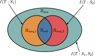
Figure 1: Partial Information Decomposition reveals the intricate interdependencies between classical information-theoretic quantities [4]. Using PID, the mutual information $I(T:S_{1},S_{2})$ (large oval) and the marginal information terms $I(T:S_{1})$ and $I(T:S_{2})$ (circles) can simultaneously be dissected into a total of four information atoms (colored areas): The unique information that $S_{1}$ carries about $T$, $\Pi_{\mathrm{unq,1}}$ (orange), and likewise the unique information of $S_{2}$, $\Pi_{\mathrm{unq,2}}$ (red); the redundant information of $S_{1}$ and $S_{2}$ about $T$, $\Pi_{\mathrm{red}}$ (blue), and the synergistic information exclusively contained in $S_{1}$, and $S_{2}$, $\Pi_{\mathrm{syn}}$ (teal). The marginal mutual information terms $I(T:S_{i})$ can be constructed from the redundant and the corresponding unique atoms, while the joint mutual information $I(T:S_{1},S_{2})$ contains of all four atoms.

To provide a succinct account of the PID problem and its intuitive meaning, we start with a discussion of PID using only two source variables—referred to as bivariate PID—in this section. A comprehensive treatment of the general multivariate PID is deferred to Section III.

The mutual information $I(T:\bm{S})$ that two source variables $\bm{S}=(S_{1},S_{2})$ hold about a target variable $T$ can be conveyed by the source variables in four distinct ways (see Figure 1): Some parts of the information might be unique to either $S_{1}$ or $S_{2}$, meaning they are inaccessible from the other variable. Other parts may be redundant between both, meaning that they can be obtained from either source, while finally some parts only become accessible synergistically when both sources are observed together—like a cipher text and its corresponding password are jointly necessary to recover the plain text. We denote these PID atoms by $\Pi_{\mathrm{unq,1}}$ and $\Pi_{\mathrm{unq,2}}$ for the unique information, by $\Pi_{\mathrm{red}}$ for the redundant information, and by $\Pi_{\mathrm{syn}}$ for the synergistic information.

To understand how the joint mutual information $I(T:\bm{S})$ relates to the PID atoms, a first step is to look at the marginal mutual information terms $I(T:S_{1})$ and $I(T:S_{2})$, which quantify the statistical dependence between the target $T$ and a single source variable. These two information quantities, however, need not be disjoint, because each mutual information, while containing the respective unique atoms $\Pi_{\mathrm{unq,1}}$ or $\Pi_{\mathrm{unq,2}}$, also contain the redundant atom $\Pi_{\mathrm{red}}$. Finally, besides the two unique and the redundant term, the joint mutual information $I(T:\bm{S})$ also contains the synergistic atom $\Pi_{\mathrm{syn}}$, which is part of neither of the marginal mutual information terms because it is inaccessible from any single source alone. These requirements lead to the so-called consistency equations for two source variables [4, 5]:

$$I(T:S_{1}) =\Pi_{\mathrm{red}}+\Pi_{\mathrm{unq,1}}$$ (1)

$$I(T:S_{2}) =\Pi_{\mathrm{red}}+\Pi_{\mathrm{unq,2}}$$

$$I(T:\bm{S}) =\Pi_{\mathrm{red}}+\Pi_{\mathrm{unq,1}}+\Pi_{\mathrm{unq,2}}+\Pi_{\mathrm{syn}}\,.$$

Note that, in the bivariate case, there are four unknown PID atoms, yet only three consistency equations providing constraints. Hence, the system is underdetermined and has to be resolved by defining an additional quantity. Typically, this is done by explicitly quantifying the redundancy $\Pi_{\mathrm{red}}$ (e.g., [4, 27, 26]). For more than two source variables, a generalized notion of redundancy $I_{\cap}$ needs to be introduced which captures the redundancy between sets of source variables (see Section III.1).

In recent years, a variety of different redundancy measures has been suggested which fulfill a number of partly incompatible assumptions and have different operationalizations, e.g. from decision [25] or game theory [28]. In this work, we focus on the $I^{\mathrm{sx}}_{\cap}$ redundancy measure [26], which is rooted in the probability- and information-theoretic considerations of Fano [2].

II.1 The $I^{\mathrm{sx}}_{\cap}$ redundancy measure and the measure-theoretic definition of continuous $I^{\mathrm{sx}}_{\cap}$

The $I^{\mathrm{sx}}_{\cap}$ redundancy measure has originally been defined for discrete random variables [26]. To understand the intuition behind the definition, consider a discrete target random variable $T$ and two discrete source random variables $S_{1}$ and $S_{2}$, taking on realizations $t$ and $(s_{1},s_{2})$, respectively.

Notice that the joint mutual information $I(T:S_{1},S_{2})$ between the target and both sources can be written as an expectation value of local mutual information terms $i(t:s_{1},s_{2})$ as [3]

$$I(T:S_{1},S_{2})=\sum_{t,s_{1},s_{2}}p_{T,S}(t,s_{1},s_{2})\,i(t:s_{1},s_{2})\,,$$ (2)

where

$$i(t:s_{1},s_{2}) =\log_{2}\left[\frac{p_{T|S}(t|s_{1},s_{2})}{p_{T}(t)}\right]$$ (3a)

$$=\log_{2}\left[\frac{p_{T|S}(t|S_{1}=s_{1}\land S_{2}=s_{2})}{p_{T}(t)}\right]\,.$$ (3b)

The local mutual information reflects how we need to update our beliefs about the occurrence of the target event $T=t$ when we know both source events $S_{1}=s_{1}$ and $S_{2}=s_{2}$ have occurred [2]: If knowledge of the event $S_{1}=s_{1}$ and $S_{2}=s_{2}$ happening increases the likelihood of guessing the correct target event $T=t$ (i.e., $p_{T|S_{1},S_{2}}(t|s_{1},s_{2})>p_{T}(t)$), the event is called informative and $i(t:s_{1},s_{2})$ is positive. Vice versa, if one is less likely to guess the target event $T=t$ after knowing the source events (i.e., $p_{T|S_{1},S_{2}}(t|s_{1},s_{2})<p_{T}(t)$), the event is called misinformative and $i(t:s_{1},s_{2})<0$.

In the second transformation step (see Equation 3b) we explicitly state the logical statement whose observation leads us to update our beliefs about $T=t$. Makkeh et al. [26] suggest that building on this basic idea, a measure for redundancy can be constructed by instead measuring how our beliefs about $T=t$ are updated if we only know that either $S_{1}=s_{1}$ or $S_{2}=s_{2}$ have occurred, which leads to the local expression

$$i_{\cap}^{\mathrm{sx}}(t:s_{1};s_{2})=\log_{2}\left[\frac{p(t|S_{1}=s_{1}\lor S_{2}=s_{2})}{p(t)}\right]\,.$$ (4)

Averaging this quantity with weights $p(t,s_{1},s_{2})$ as in Equation 2 then yields a global measure of redundant information between sources $S_{1}$ and $S_{2}$ about $T$, denoted by $I^{\mathrm{sx}}_{\cap}$, i.e., [26]

$$I^{\mathrm{sx}}_{\cap}=\sum_{s_{1},s_{2},t}p(t,s_{1},s_{2})\;i_{\cap}^{\mathrm{sx}}(t:s_{1};s_{2})\,.$$ (5)

This redundancy measure is symmetric with respect to swapping the sources $S_{1}$ and $S_{2}$ and invariant towards any arbitrary bijective relabelling of the discrete realizations of any of the random variables. Furthermore, it fulfills a target chain rule and is differentiable with respect to the underlying probability distribution [26].

Equivalently, Definition 2 can be derived from the regions of probability space which $S_{1}=s_{1}$ and $S_{2}=s_{2}$ jointly render impossible (see Appendix A), which is why the PID definition is referred to as “shared exclusion PID”. For more than two source variables, the logical expression in the numerator has to be extended to account for disjunctions between sets of source events occurring simultaneously (see Section III.2).

In previous work, Schick-Poland et al. [34] showed that the $I^{\mathrm{sx}}_{\cap}$ redundancy measure can be generalized to continuous source and target variables. In particular, the authors proved the existence of a measure-theoretic generalization of $I^{\mathrm{sx}}_{\cap}$, which can handle arbitrarily many source variables while being invariant under isomorphic transformations and differentiable with respect to the joint distribution of sources and target. The proof of the existence of this generalization builds on established theorems from probability and measure theory. It is shown that the derived measure inherits all the above mentioned desirable properties of the discrete $I^{\mathrm{sx}}_{\cap}$ measure and is applicable to any possible discrete or continuous variable settings.

However, due to the provided proofs not being entirely constructive, a rigorous analytic formulation of this continuous $I^{\mathrm{sx}}_{\cap}$ measure remains elusive. While proven to exist from measure-theoretic principles, the way to construct a transformation-invariant shared-exclusion redundancy measure remains unclear. Therefore, in the next section we provide an analytical definition for a purely continuous $I^{\mathrm{sx}}_{\cap}$ measure which, while not adhering to all properties described by Schick-Poland et al. [34], provides a practical and interpretable shared-exclusion based continuous PID definition. In the following, we show how such a formulation can be obtained, present an estimation procedure and discuss its relation to the measure-theoretic derivation.

II.2 An analytical formulation of a continuous $I^{\mathrm{sx}}_{\cap}$ measure

II.2.1 Definition

To make a continuous $I^{\mathrm{sx}}_{\cap}$ measure available to practitioners, an important first step is to find an analytic formulation. In this section, we present such a formulation and show how it can be computed numerically for a given probability density function. Since in most practical applications one has only access to a finite sample of data from an unknown distribution, we introduce an estimator for this redundancy measure based on k-nearest-neighbour distances in Section II.3.

The main difficulty for finding an analytical formulation for the continuous $I^{\mathrm{sx}}_{\cap}$ measure is due to the disjunction (logical “or”) in Definition 2. While conjunctions (logical “and”) are ubiquitous in classical continuous information theory and correspond to simple joint probability densities, disjunctive statements have no established counterpart in the continuous regime. In the following we will introduce an intuitive notion of how such a measure can be defined, while we defer a rigorous derivation to Appendix F.

For discrete random variables, the probability of the event $S_{1}=s_{1}\lor S_{2}=s_{2}$ is given by the inclusion-exclusion-rule as

$$\begin{gathered}\mathbb{P}(S_{1}=s_{1}\lor S_{2}=s_{2})\\ =p_{S_{1}}(s_{1})+p_{S_{2}}(s_{2})-p_{S_{1},S_{2}}(s_{1},s_{2})\,,\end{gathered}$$ (6)

where the last term $p_{S_{1},S_{2}}(s_{1},s_{2})$ is the probability of both $S_{1}=s_{1}$ and $S_{2}=s_{2}$ occurring, which is double-counted in the sum of marginals and thus needs to be subtracted once.

To make the leap from discrete to continuous variables, the probability mass functions $p_{S_{i}}$ of Equation 6 can be reinterpreted as a binned distribution of an underlying continuous probability density $f_{S_{i}}$, i.e.,

$$p(s_{i})=\int_{U_{s_{i}}}\mathrm{d}s_{i}^{\prime}\,f_{S_{i}}(s_{i}^{\prime})\approx|U_{s_{i}}|\,f_{S_{i}}(s_{i})\,,$$

where $\{U_{s_{i}}\}_{s_{i}}$ is a partition of the support of $f_{S_{i}}$ and $|U_{s_{i}}|$ is the area of one of the sets of the partition. The probability of the binned disjunction, i.e., the probability of either $S_{1}$ falling into the bin $U_{s_{1}}$ or $S_{2}$ falling into $U_{s_{2}}$ then becomes

$$\begin{gathered}\mathbb{P}(S_{1}\in U_{s_{1}}\lor S_{2}\in U_{s_{2}})\\ =|U_{s_{1}}|\,f_{S_{1}}(s_{1})+|U_{s_{2}}|\,f_{S_{2}}(s_{2})\\ -|U_{s_{1}}||U_{s_{2}}|\,f_{S_{1},S_{2}}(s_{1},s_{2})\,.\end{gathered}$$ (7)

To get to a fully continuous description, one now has to take the limit of the partitionings $\{U_{s_{1}}\}_{s_{1}}$ and $\{U_{s_{2}}\}_{s_{2}}$ becoming increasingly fine. Here, the subtracted term contains a product of bin sizes and will therefore shrink faster in this limit. Thus, it will become negligible compared to the two terms before under the assumption that $f_{S_{1},S_{2}}(s_{1},s_{2})$ is finite everywhere.

Nonetheless, neglecting the third term still leaves a choice of how the limits of the partitionings are taken with respect to each other. Intuitively, this freedom is reflective of the relative scale with which the variables are considered: Since ultimately, probability densities are defined by what finite probability masses they integrate to in small neighbourhoods, the relative scale between two variables defines how to compare the neighborhoods for two variables. If the two marginal distributions of the sources are the same, a canonical choice is to take the same partitioning for both variables. On the other hand, if the variables come from very different distributions, the variables might need to be transformed to a comparable scale by a suitable preprocessing step.

Note that this ansatz is closely related to the introduction of differential entropy by Jaynes [36]. Jaynes similarly arrives at the conclusion that when rigorously deriving the differential entropy from an analogous limit process, there remains some freedom of choice in the final definition which he captures in what he terms the “limiting density of discrete points”. This limiting density may be understood as a function indicating the local measurement scales, which cannot be excluded from the differential entropy. Only in the case of the continuous mutual information, these terms cancel exactly, leaving a unique and transformation-invariant measure.

Table 1: Numerical evaluations for four example distributions show qualitative similarities between discrete and the continuous $I^{\mathrm{sx}}_{\cap}$ on the three selected logic gates, while qualitative differences can be observed for the sum example. In the continuous case, the sources are distributed normally, $S_{i}\sim\mathrm{Normal}(\mu=0,\sigma=1)$, except for $S_{2}$ in the redundant gate which is set equal to $S_{1}$, and the target is constructed according to the pictograms with added Gaussian noise ($\sigma=0.01$) to make the mutual information $I(T:S_{1},S_{2})$ finite. In the discrete setting, the variables are drawn from uniform binary distributions and no noise is added to the target.

	Redundant Gate	Copy Gate	Unique Gate	Sum
Continuous Gates
$\Pi_{\mathrm{syn}}$	$0.000\,\mathrm{bits}$	$6.644\,\mathrm{bits}$	$5.525\,\mathrm{bits}$	$6.497\,\mathrm{bits}$
$\Pi_{\mathrm{unq,1}}$	$0.000\,\mathrm{bits}$	$0.000\,\mathrm{bits}$	$1.119\,\mathrm{bits}$	$0.147\,\mathrm{bits}$
$\Pi_{\mathrm{unq,2}}$	$0.000\,\mathrm{bits}$	$0.000\,\mathrm{bits}$	$-5.525\,\mathrm{bits}$	$0.147\,\mathrm{bits}$
$\Pi_{\mathrm{red}}$	$6.644\,\mathrm{bits}$	$6.644\,\mathrm{bits}$	$5.525\,\mathrm{bits}$	$0.353\,\mathrm{bits}$
$I(T:S_{1},S_{2})$	$6.644\,\mathrm{bits}$	$13.288\,\mathrm{bits}$	$6.644\,\mathrm{bits}$	$7.144\,\mathrm{bits}$
Discrete Gates
$\Pi_{\mathrm{syn}}$	$0.000\,\mathrm{bits}$	$0.415\,\mathrm{bits}$	$0.415\,\mathrm{bits}$	$0.415\,\mathrm{bits}$
$\Pi_{\mathrm{unq,1}}$	$0.000\,\mathrm{bits}$	$0.585\,\mathrm{bits}$	$0.585\,\mathrm{bits}$	$0.585\,\mathrm{bits}$
$\Pi_{\mathrm{unq,2}}$	$0.000\,\mathrm{bits}$	$0.585\,\mathrm{bits}$	$-0.415\,\mathrm{bits}$	$0.585\,\mathrm{bits}$
$\Pi_{\mathrm{red}}$	$1.000\,\mathrm{bits}$	$0.415\,\mathrm{bits}$	$0.415\,\mathrm{bits}$	$-0.085\,\mathrm{bits}$
$I(T:S_{1},S_{2})$	$1.000\,\mathrm{bits}$	$2.000\,\mathrm{bits}$	$1.000\,\mathrm{bits}$	$1.500\,\mathrm{bits}$

How the variables should be preprocessed, if at all, depends on the nature of the variables in question. For instance, if two variables measure the same physical quantity but with different scales, e.g. body height measured in centimeters versus in feet, a reasonable preprocessing step would be the rescaling of one of the variables or—if the variables come from a similar distribution—a standardization of both. Alternatively, if the precision can be assumed to be proportional to the probability density at that point, the original probability densities $f$ may be replaced with the copula densities $c$, which furthermore happens to make the measure invariant under invertible mappings of individual variables before this step.

Finally, these considerations lead to the following definition for the probability of a continuous disjunction for two random variables $S_{1}$ and $S_{2}$, which have possibly been preprocessed beforehand.

Definition 1.

Let $S_{1},S_{2}$ be continuous random variables with associated densities $f_{S_{1}},f_{S_{2}}$. Then we define the quasi-density of the disjunctive logic statement $S_{1}=s_{1}\lor S_{2}=s_{2}$ to be

$$f_{S_{1}\lor S_{2}}(s_{1}\lor s_{2}):=f_{S_{1}}(s_{1})+f_{S_{2}}(s_{2})\,.$$

Note that in the above definition, it is assumed that the precision of one variable does not depend on the value of the other variable and that the relative precision between the two variables is constant. Furthermore, while the local density of a disjunction as defined above does not fulfill all properties of a density function in the mathematical sense (particularly, it does not integrate to one), it nevertheless serves as a local approximate proportionality of probability in relation to magnitude of area in state space.

Given this definition for a continuous disjunction, we can write down an analytical formulation for the continuous local shared-exclusion redundancy.

Definition 2.

Let $S_{1},S_{2}$ be continuous random variables with associated densities $f_{S_{1}},f_{S_{2}}$.

Then we define the continuous local shared-exclusion redundancy for two sources as

$$i^{\mathrm{sx}}_{\cap}(t,\{s_{1}\}\{s_{2}\}):=\log_{2}\frac{f_{T|S_{1}\lor S_{2}}(t|s_{1}\lor s_{2})}{f_{T}(t)}$$

$$=\log_{2}\frac{f_{T,S_{1}}(t,s_{1})+f_{T,S_{2}}(t,s_{2})}{f_{T}(t)(f_{S_{1}}(s_{1})+f_{S_{2}}(s_{2}))}.$$

This measure for continuous redundancy shares many of the favourable properties of its discrete counterpart. In particular, it is localizable (i.e., it can be expressed as an expected value of local values) and can be generalized to arbitrary numbers of source variables (see Section III). Furthermore, the continuous $i^{\mathrm{sx}}_{\cap}$ measure is differentiable with respect to the underlying probability density function (see Appendix B).

As in the case of the mutual information, the average redundancy is defined as the expectation value of the local values, i.e.,

$$I^{\mathrm{sx}}_{\cap}(T,\{S_{1}\}\{S_{2}\})$$

$$=\int\mathrm{d}t\,\mathrm{d}s_{1}\,\mathrm{d}s_{1}\,f_{T,S_{1},S_{2}}(t,s_{1},s_{2})\,i^{\mathrm{sx}}_{\cap}(t,\{s_{1}\}\{s_{2}\}).$$

Finally, given this quantification of the redundant information in conjunction with the three classical mutual information terms between $T$ and the sources, the four information atoms can be computed by solving Equation 1, which in the general case is known as a Moebius Inversion [4] (see Section III.1).

II.2.2 Results for toy examples

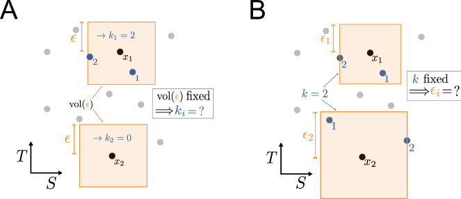
Figure 2: Local densities can be estimated from data in two opposite ways. A Kernel density estimation using a fixed volume $\mathrm{vol}(\epsilon)$ around the reference point $x_{i}$. B $k$-nearest-neighbor-based estimation using an adaptive search volume, determined by the distance to the $k$-th neighbor.

To gain an intuition for the continuous $I^{\mathrm{sx}}_{\cap}$ measure, we apply the analytical formulation established in the previous section to simple and intuitive toy examples. Such simple example cases can be found in logic gates, which have been employed as examples for discrete PID measures throughout the literature (e.g., [25, 37]). We here use continuous versions of the well-established “redundant”, “unique” and “copy” gate as well as a sum between source variables and discuss the results compared to their discrete counterparts. In the discrete domain, the two source variables are binary with two equiprobable realizations, whereas in the continuous domain, we draw the variables from a standard normal distribution. To ensure a finite mutual information, which guarantees a well-defined continuous PID, Gaussian noise with standard deviation $\sigma=0.01$ is added to the target variable $T$ in the continuous case.

While some logic gates (like the “and” gate) have no canonical continuous counterparts, we selected three gates whose basic concept can be straightforwardly transferred to the continuous domain: The redundant gate, in which the two sources are the same and equal to the target, the copy gate, in which the target is a joint variable consisting of the two source variables, and the unique gate, in which the target is a copy of the first source variable while the second source variable is drawn independently from the target. In addition to the three logic gates, we added the “sum” example, in which the target variable is the sum of the two sources.

While the computation of the discrete PID atoms is a straightforward exercise, the computation of the continuous atoms is more difficult due to the integral expressions. Note, first, that all continuous examples can be expressed as multivariate Gaussian distributions (see Appendix C), for which an analytical closed form for the joint and marginal mutual information terms exists [3]. The integrals involved in computing the redundancy, however, cannot be easily evaluated analytically. Therefore, we resorted to simple Monte Carlo integration techniques to numerically estimate the involved integrals. To compute the expectation value, we drew randomly from the given joint probability distributions, and computed the local $i^{\mathrm{sx}}_{\cap}$ redundancy for $10^{8}$ samples. The PID atoms can then be computed from the analytical mutual information and the numerically computed redundancy via the consistency equations (see Equation 1).

Table 1 shows the results for all four examples. Note that $I^{\mathrm{sx}}_{\cap}$, as an information measure constructed for quantifying redundant information, assigns all the information that exists between the variables for the redundant gate to redundant information. This behavior is expected since the probability of a disjunction between two equal events, e.g. $S_{1}=s_{1}\lor S_{1}=s_{1}$ is trivially equal to just the probability of one of the events.

For the three logic gates, the discrete and continuous PID results share many qualitative similarities. As mentioned, in both settings all information is attributed to redundancy for the redundant gate, while also the synergy is equal to the redundancy in the copy and the unique gate. Further similarities are that for the unique gate, the unique information of source $S_{1}$ is positive while the unique information of $S_{2}$ is negative. For the “sum” example, however, the discrete and continuous examples differ qualitatively: While in the discrete case, the unique atoms are positive while the redundancy is negative, all atoms are positive in the continuous case. These discrepancies are likely due to the fact that the discrete Sum gate is not a good analogue of the continuous case, since the values of the realizations the discrete random variable can take on has no natural total ordering.

Depending on the setting that the variables arise in, different preprocessing schemes might need to be applied to the variables before computing the PID atoms. Using different preprocessing schemes, one finds that the values agree qualitatively on most gates, which is mostly due to them being drawn from the same distributions. For a more detailed discussion, refer to Appendix G.

II.3 KSG nearest-neighbour based estimator for mutual information

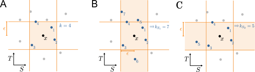
Figure 3: The KSG estimator for mutual information [35] works by considering $k$th nearest neighbors in the joint and marginal spaces in three steps. A Determining search radius in joint space B counting neighbors in marginal space of $S$ and C counting neighbors in marginal space of $T$.

While we established in Section II.2 how continuous $I^{\mathrm{sx}}_{\cap}$ can be computed from a given probability distribution, in most research settings this distribution is unknown. More commonly, one has access to only a finite sample drawn from this distribution and needs to estimate the information-theoretic quantities of interest from this sample. For mutual information, several different approaches to this estimation problem have been discussed in literature, for instance, binning or kernel density estimation (see, e.g., [38] for a review). However the nearest-neighbour-based approach introduced by Kraskov, Stögbauer and Grassberger [35] (KSG) has been widely adopted due to its favourable variance-bias characteristics. In the following, we explain how local probabilities can be estimated using nearest-neighbor techniques [39] and introduce the key ideas behind the KSG estimator. Then, we show how these concepts can be built upon to derive an estimator for continuous $I^{\mathrm{sx}}_{\cap}$.

Many information-theoretic quantities like the mutual information (see Equation 2) can be expressed as expectation values of local quantities. For discrete data, a simple (but not optimal [40]) way to approximate these local values is to replace the probability masses by their frequencies in the sample, which is referred to as plug-in estimation. In the continuous case, however, all samples are almost always unique, which is why no continuous analogue to the plug-in principle exists. Thus, one has to revert to more elaborate methods to estimate the local densities $f(x_{i})$ necessary for computing the local information-theoretic values.

Nearest-neighbor-based estimation of local probability densities

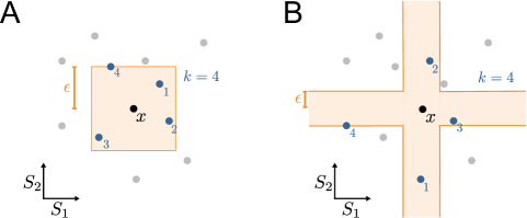
Figure 4: To estimate local redundant information for a two-variable example, the search regions of the original mutual information KSG estimator [35] need to be adapted. A For mutual information estimation, the radius $\epsilon$ at a point $x$ is assessed in the joint space by searching for the minimal distance such that all of the variables’ marginal distances to $x$ is smaller or equal to $\epsilon$. B For redundancy estimation, on the other hand, $\epsilon$ is inferred by searching for the minimal distance such that at least one of the variables’ marginal distances to $x$ is smaller or equal to $\epsilon$.

To estimate the local probability densities at the sample points, we exploit the intuitive idea that sample points are more likely to be closer together in regions of higher probability density. Note that this intuition crucially rests on the assumption that the sample is sufficiently large such that the true probability density varies only little between neighbouring data points. If this prerequisite is met, a natural approach to estimate the local probability density is to take a ball $B_{\epsilon}(x_{i})$ of fixed radius $\epsilon$ around the evaluation point $x_{i}$, over which the probability density is assumed to be approximately constant, and count the number of neighbours $k_{i}$ within the ball (see Figure 2.A). A point estimate for the probability density is then given by the fraction of sample points $(k_{i}+1)/N$ within that $\epsilon$-ball divided by its volume $\mathrm{vol}(B_{\epsilon}(x_{i}))$ as

$$\hat{f}(x_{i})=\frac{k_{i}+1}{N\mathrm{vol}(B_{\epsilon}(x_{i}))}\,.$$ (8)

Kernel density estimators (KDE) use this principle, but typically weigh the neighbors by their respective distance using a fixed kernel, which in general does not have to be the characteristic function of an $\epsilon$-neighborhood.

The disadvantage of approaches like this is that the same ball or kernel is used irrespective of the local density: In areas of low density there may be insufficiently many points within the neighborhood to arrive at a good estimation, while conversely in areas of high density the high numbers $k_{i}$ would have allowed for a smaller search region, partly relaxing the smoothness assumption on $f$. A way to get around these problems is to invert the procedure: Instead of fixing the search radius $\epsilon$ and counting the number of neighbouring points $k_{i}$, one can fix a natural number $k$ and compute the distance $\epsilon_{i}$ from point $x_{i}$ to its $k$-th nearest neighbor (see Figure 2.B). Analogously to Equation 8, a point estimate of the local probability density can now be expressed as

$$\hat{f}(x_{i})=\frac{k+1}{N\mathrm{vol}(B_{\epsilon_{i}}(x_{i}))}\,.$$ (9)

The Kozachenko-Leonenko (KL) Estimator for Shannon Differential Entropy

Kozachenko and Leonenko [39] used the nearest-neighbour-based approach to build an estimator for the Shannon differential entropy [3]

$$H(X)=\mathbb{E}[-\log_{2}p(X)]=-\int\mathrm{d}x\,p(x)\log_{2}p(x)\,.$$ (10)

However, instead of using the point estimate of Equation 9, the authors derive the expectation value for $\log p(x_{i})$ for the probability mass of the $\epsilon$-ball

$$p(x_{i})=\int_{B_{\epsilon_{i}}(x_{i})}\mathrm{d}x^{\prime}\,f(x^{\prime})\approx\mathrm{vol}(B_{\epsilon_{i}}(x_{i}))f(x_{i})$$

given the number of neighbours $k$ for each sample point, which results in the expression

$$\widehat{\log p_{X}(x_{i})}=\psi(k)-\psi(N)\,,$$

where $\Psi$ represents the Digamma function. Plugging this result into Equation 10, the authors obtain an estimator for the Shannon differential entropy as (for a more formal derivation, refer to Appendix D)

$$\begin{gathered}\hat{H}(X)=-\frac{1}{N}\sum\limits_{i=1}^{N}\widehat{\log\left[p_{X}(x_{i})\right]}\\ =-\psi(k)+\psi(N)+\frac{1}{N}\sum\limits_{i=1}^{N}\log\left[\mathrm{vol}\left(B_{\epsilon_{i}}\right)\right]\,.\end{gathered}$$ (11)

The Kraskov-Stögbauer-Grassberger (KSG) Estimator for Mutual Information

The most straightforward way to construct an estimator for continuous mutual information from the results of Kozachenko and Leonenko [39] is by using the identity $I(T:S)=H(T)+H(S)-H(T,S)$. However, in doing so, the biases of the individual entropy estimates likely do not cancel, which led Kraskov et al. [35] to take a different approach: First, like for the KL estimator, the distance $\epsilon_{i}$ of point $x_{i}=(t_{i},s_{i})$ to its $k$th nearest neighbour is determined in the joint space (see Figure 3.A). Subsequently, the number of neighbours $n_{T}$ which have a distance of less than $\epsilon_{i}$ in only the marginal space of the first variable $T$ is determined (see Figure 3.B), and the procedure is repeated analogously to determine the number of neighbors $n_{S}$ in radius $\epsilon_{i}$ in the marginal space of the second random variable $S$ (see Figure 3.C). The advantage of obtaining the marginal probability densities using the distance determined in the joint space is that—when using the maximum norm—the volume terms which appear in Equation 11 cancel exactly, leading to the succinct expression

$$\hat{I}(T:S)=\Psi(k)+\Psi(N)-\left<\Psi(n_{T}(i))+\Psi(n_{S}(i))\right>_{i}\,,$$ (12)

for the estimated mutual information. Here, angled brackets $\left<\cdot\right>_{i}$ denote the average over the sample points.

II.4 Generalizing the KSG estimator for $I^{\mathrm{sx}}$

Adapting local probability density estimation for redundant information

To understand how to estimate the continuous redundancy $I^{\mathrm{sx}}_{\cap}$ using an approach similar to Kraskov et al. [35]’s, first consider the case of estimating the mutual information $I(T:\bm{S})$ between a single target random variable $T$ and two joint source variables $\bm{S}=(S_{1},S_{2})$ using the KSG estimator. In the first step, the radius $\epsilon_{i}$ is determined as the smallest radius in the joint space for which the $k$-th neighbor of the point $x_{i}=(t_{i},s_{1,i},s_{2,i})$ lies within the Ball $B_{\epsilon_{i}}(x_{i})$. Choosing the maximum norm, this ball in the joint space is equal to the product of the $\epsilon$-balls in the marginal spaces, i.e., $B_{\epsilon_{i}}(t_{i})\crossproduct B_{\epsilon_{i}}(s_{1,i})\crossproduct B_{\epsilon_{i}}(s_{2,i})$ (square region in Figure 4.A). In the second step, neighbours are counted within the marginal space of $\bm{S}$, where only those points are counted which lie within less than the distance $\epsilon_{i}$ to $x_{i}$ in both dimensions $S_{1}$ and $S_{2}$ simultaneously.

As laid out in detail in Section II.2, the difference in the mathematical formulation between mutual information and $I^{\mathrm{sx}}_{\cap}$ redundancy is that while the former is expressed with conjunctions, which amount to intersections of source events in sample space, the latter deals with disjunctions, which result in unions. The KSG estimator can be readily adapted to this concept by changing the search regions accordingly: To compute the redundancy in the example case of two source variables introduced above, the radius $\epsilon_{i}$ now has to be determined not as the smallest radius laying on the intersection of $B_{\epsilon_{i}}(t_{i})$, $B_{\epsilon_{i}}(s_{1,i})$ and $B_{\epsilon_{i}}(t_{2,i})$ (“square” region in Figure 4.A) but on the union of the source variable neighbourhoods intersected with the target ball $B_{\epsilon_{i}}(t_{i})\crossproduct B_{\epsilon_{i}}(s_{1,i})\crossproduct S_{2}\cup B_{\epsilon_{i}}(t_{i})\crossproduct S_{1}\crossproduct B_{\epsilon_{i}}(s_{2,i})$ (“cross” region in Figure 4.B). Similarly, $n_{S}$ is determined by counting all points which lie within the union of marginal balls with radius $\epsilon$.

Nearest-neighbor-based estimator for continuous redundant information

Adapting the steps by Kraskov et al. [35] using the described estimation procedure for the probability density of a logical disjunction we find

$$\begin{gathered}\hat{I}^{sx}_{\cap}(T:X,Y)=\langle\widehat{\log[f^{i}_{T,X\lor Y}(t,x,y)]}\rangle_{i}\\ -\langle\widehat{\log[f^{i}_{X\lor Y}(x,y)]}\rangle_{i}-\langle\widehat{\log[f^{i}_{T}(t)]}\rangle_{i}\\ =\psi(k)+\psi(N)-\langle\psi(n_{X\lor Y}(i))\rangle_{i}-\langle\psi(n_{T}(i))\rangle_{i}\,.\end{gathered}$$ (13)

More precisely, we have retaken the approach of choosing the $\epsilon$ to be determined by a nearest neighbor search in the joint space. We then use the same $\epsilon$ in the marginal spaces themselves, such that the volume terms cancel exactly. The search with the predetermined $\epsilon$ will then cause an adapted number of nearest neighbors in the marginal spaces, denoted by $n_{X\lor Y}(i)$ and $n_{T}(i)$, respectively. The exact steps leading to Equation 13 are outlined in Appendix H. Furthermore, details of the implementation and code availability are described in Appendix I.

Note, however, one subtle difference in the meaning of the parameter $\epsilon$ between the mutual information and redundancy case: While scaling $\epsilon$ by a constant factor for one but not the other source variable changes the estimated mutual information for any finite sample, it does not change what the mutual information estimator converges to in the limit of infinite samples. This is different in the case of redundancy: Because of the addition of marginal densities in Definition 1, scaling one but not the other search radius $\epsilon$ makes a difference also in the limit of infinite samples. Using the same $\epsilon$ for both source variables here thus reflects the choice of treating the source variables on “equal footing”.

II.5 Convergence of the estimator for simple toy examples

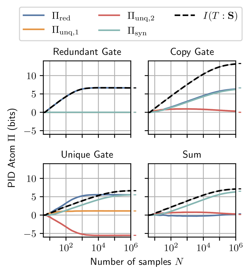
Figure 5: With increasing sample size $N$, the estimated PID atoms converge to the numerically evaluated analytical results. The subfigures show the four PID atoms $\Pi$ and the mutual information $I(T:\bm{S})$ for the continuous redundant, unique and copy gates as well as the sum example estimated using the nearest-neighbors approach outlined above with $k=4$. The colored bars to the right of the graphs correspond to the respective analytical value for each atom and gate from Table 1.

In order to assess the efficacy of our estimation procedure, we applied it to the toy examples outlined in Section II.2. To this end, different numbers of samples have been drawn from the known probability distributions and have been plugged into the estimator to check for convergence.

Figure 5 shows how the PID atoms converge with more samples for the four example cases. The copy gate and sum example converge slower than the other values. This behaviour is inherited from the KSG estimator, which also converges more slowly for higher-dimensional distributions and distributions with higher mutual information. All in all, we conclude that the estimator succeeds in reproducing the numerically evaluated analytical results from Section II.2 given sufficiently many samples.

III Definition of multivariate continuous $I^{\mathrm{sx}}_{\cap}$

III.1 The multivariate PID Problem

In the previous sections we introduced the continuous $I^{\mathrm{sx}}_{\cap}$ measure for two source variables. However, as was already mentioned, the PID framework as envisioned by Williams and Beer [4] is more general and in principle applicable to an arbitrary number of sources. In the following, we will explain the PID problem for the general, multivariate case and generalize the continuous $I^{\mathrm{sx}}_{\cap}$ measure accordingly. This section may be skipped if the reader has a particular application in mind for which two source variables suffice and this section is found too technical.

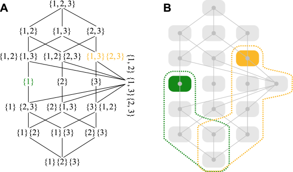
Figure 6: The PID lattice structure for three source variables reveals how generalized redundancies can be dissected into PID atoms [4, 5]. A Every node in the redundancy lattice represents a generalized redundancy $I_{\cap}$ for a given antichain, while edges indicate parthood of generalized redundant information in information terms higher up the lattice. For instance, the mutual information $I(T:S_{1})$, which corresponds to the self-redundancy with the antichain $\{1\}$, contains all redundancies in its downset, i.e., those with antichains $\{1\}\{2,3\}$, $\{1\}\{2\}$, $\{1\}\{3\}$ and $\{1\}\{2\}\{3\}$, which, however, themselves overlap and contain parts of each other. B The PID atoms (shaded boxes), which are referenced by the same antichains, only comprise the information that the redundancy of the same antichain contains in excess of what the all the atoms below contain together. Atoms thus reflect the incremental increases of the redundancies which conversely can be used to construct the generalized redundancies. For instance, the redundancy with antichain $\{1\}$ is the sum of the four atoms in its downset plus the atom $\{1\}$ itself (green shaded box and green dashed outline, respectively). Analogously, the figure shows how the redundancy with the antichain $\{1,3\}\{2,3\}$ (orange) is constructed from the atoms in its downset.

Before we generalize to an arbitrary number of source variables, note that already in the bivariate case, each atom can be uniquely identified by which mutual information terms it contributes to via the consistency equations (see Equation 1). For instance, the unique atom $\Pi_{\mathrm{unq,1}}$ is the only atom that is part of both $I(T:S_{1})$ and $I(T:\bm{S})$ but not $I(T:\bm{S}_{2})$ while the synergistic information atom $\Pi_{\mathrm{syn}}$ is precisely the one atom whose information is contained in neither $I(T:S_{1})$ nor in $I(T:S_{2})$, but only in $I(T:S_{1},S_{2})$. In the following, we show how this notion of parthood, also called mereology, can serve as a general framework for identifying and ordering PID atoms for arbitrarily many source variables [5].

Mathematically, the mereological relations between an atom and the marginal mutual information terms can be captured by a parthood distribution $\Phi:\mathcal{P}(\bm{S})\rightarrow\{0,1\}$: A boolean function defined on the power set of source variables $\mathcal{P}(\bm{S})$ which is equal to $1$ for exactly those sets of sources $\bm{S}_{\bm{a}}=\{S_{i}\mid i\in\bm{a}\}$ for which the atom $\Pi_{\Phi}$ is part of the marginal mutual information $I(T:\bm{S}_{\bm{a}})$ [5]. Note that not all boolean functions constitute valid parthood distributions: Since all information about $T$ that is contained the mutual information $I(T:\bm{S}_{\bm{a}})$ with a set of sources $\bm{S}_{\bm{a}}$ must naturally also be contained in the mutual information $I(T:\bm{S}_{\bm{b}})$ with any superset $\bm{S}_{\bm{b}}\supset\bm{S}_{\bm{a}}$, $\Phi$ has to be monotone, in the sense that $\bm{S}_{\bm{b}}\supset\bm{S}_{\bm{a}}\Rightarrow(\Phi(\bm{S}_{\bm{a}})=1\to\Phi(\bm{S}_{\bm{b}})=1)$. For instance, any information provided by source $S_{1}$ alone must naturally also be present when taking sources $S_{1}$ and $S_{2}$ together. Furthermore, we must always require that $\Phi(\emptyset)=0$ and $\Phi(\bm{S})=1$, indicating that no atom is part of the mutual information with the empty set and, conversely, all information atoms are part of the full joint mutual information $I(T:\bm{S})$.

The marginal mutual information terms can be constructed additively from these PID atoms according to the generalized consistency equations

$$I(T:\bm{S}_{\bm{a}})=\sum_{\Phi:\Phi(\bm{S}_{\bm{a}})=1}\Pi_{\Phi}\,.$$ (14)

The number of such parthood distributions, and thus of the PID atoms, grows superexponentially like the Dedekind numbers [5]. On the other hand, there are only $2^{n}-1$ classical mutual information quantities providing constraints through Equation 14, leaving these consistency equations underdetermined and making it impossible to determine the sizes of the PID atoms. This underdeterminedness is typically resolved by introducing a measure for generalized redundancy $I_{\cap}(T:\bm{S}_{\Phi})$ for each parthood distribution $\Phi$. This redundancy generalizes the mutual information and fulfills

$$I_{\cap}(T:\bm{S}_{\Phi})=\sum_{\Psi:\Psi\prec\Phi}\Pi_{\Psi}\,,$$ (15)

where the sum is over all atoms $\Pi_{\Psi}$ with a parthood distribution $\Psi$ which are part of the generalized redundancy $I_{\cap}(T:\bm{S}_{\Phi})$.

This condition is similar to the monotonicity requirement of the mutual information mentioned before and is mathematically captured in the ordering relation $\prec$ given by

$$\Psi\prec\Phi\Leftrightarrow\Phi(\bm{S}_{\bm{a}})=1\to\Psi(\bm{S}_{\bm{a}})=1\text{ for all }\bm{S}_{\bm{a}}\subseteq\bm{S}\,.$$

This partial ordering bestows a structure onto the set of PID atoms which is known as the “redundancy lattice” (see Figure 6).

Comparing Equations 14 and 15, one finds that the mutual information can be interpreted as a “self-redundancy”—a special case of a redundancy which describes how the mutual information provided by a set of sources about the target is trivially redundant with itself. Finally, to quantify the atoms $\Pi_{\Phi}$ given the redundancies $I_{\cap}(T:\bm{S}_{\Phi})$, Equation 15 can be inverted, which, due to the partial ordering, is known as a Moebius inversion [4].

Equivalently, each parthood distribution can be uniquely identified by the set of sets of source variables for which the parthood distribution is equal to $1$, i.e., $\Phi^{-1}[\{1\}]$. Because of the monotonicity requirement mentioned before, we can make this representation even more concise by removing all sets which are supersets of others, which gives the so-called antichains

$$\alpha=\left\{\bm{a}\in\Phi^{-1}[\{1\}]\mid\not\exists\,\bm{b}\in\Phi^{-1}[\{1\}]\text{ s.t. }\bm{b}\subseteq\bm{a}\right\}\,,$$ (16)

which is the most prevalent way how PID atoms are referred to throughout literature and also the formalism that PID was originally conceived in [4]. Throughout this paper, the outer braces of the set of sets are neglected for the sake of brevity (e.g., $\{1\},\{2\}$ instead of $\{\{1\},\{2\}\}$. The term antichain stems from the fact that the sets contained within $\alpha$ are incomparable with respect to the partial order of set inclusion. These antichains make the intuitive meaning of the redundancy terms explicit, e.g., $I_{\cap,\{1\}\{2,3\}}$ refers to the information that can either be obtained from source $S_{1}$ alone, or–redundantly to that–from sources $S_{2}$ and $S_{3}$ taken together.

III.2 Definition of multivariate continuous $I^{\mathrm{sx}}_{\cap}$

Since in the multivariate case the generalized redundancy $I_{\cap,\alpha}$ refers, for a particular antichain $\alpha$, to information that can equivalently be obtained from all sets $\bm{S}_{\bm{a}}$ for $\bm{a}\in\alpha$ of source variables taken together, the logical statement in the conditional probability of Definition 2 needs to be generalized to accommodate for such general disjunctions as

$$i_{\cap,\alpha}^{\mathrm{sx}}(t:s_{1};s_{2})=\log_{2}\left[\frac{p(t|\bigvee_{\bm{a}\in\alpha}\bm{S}_{\bm{a}}=\bm{s}_{\bm{a}})}{p(t)}\right]$$ (17)

$$=\log_{2}\left[\frac{p(t|\bigvee_{\bm{a}\in\alpha}\bigwedge_{i\in\bm{a}}S_{i}=s_{i})}{p(t)}\right]\,,$$ (18)

where $\bm{S}_{\bm{a}}=\{S_{i}\mid i\in\bm{a}\}$ and likewise $\bm{s}_{\bm{a}}=\{s_{i}\mid i\in\bm{a}\}$. This generalization is analogous to how the multivariate redundancy is introduced for the discrete case by Makkeh et al. [26].

III.3 Estimation of multivariate continuous $I^{\mathrm{sx}}_{\cap}$

To estimate multivariate continuous $I^{\mathrm{sx}}_{\cap}$, the search regions used by the nearest neighbor estimator need to be expanded to higher dimensions. For $d>2$ source variables $\bm{S}=(S_{1},\dots,S_{d})$ and a specific antichain $\alpha$, the search space for determining the radius $\epsilon_{i}$ is given by the union of intersections

$$\bigcup_{\bm{a}\in\alpha}B_{\epsilon_{i}}(t_{i})\times{}_{j\in\bm{a}}B_{\epsilon_{i}}(s_{i,j})\times{}_{j\notin\bm{a}}S_{j}\,.$$ (19)

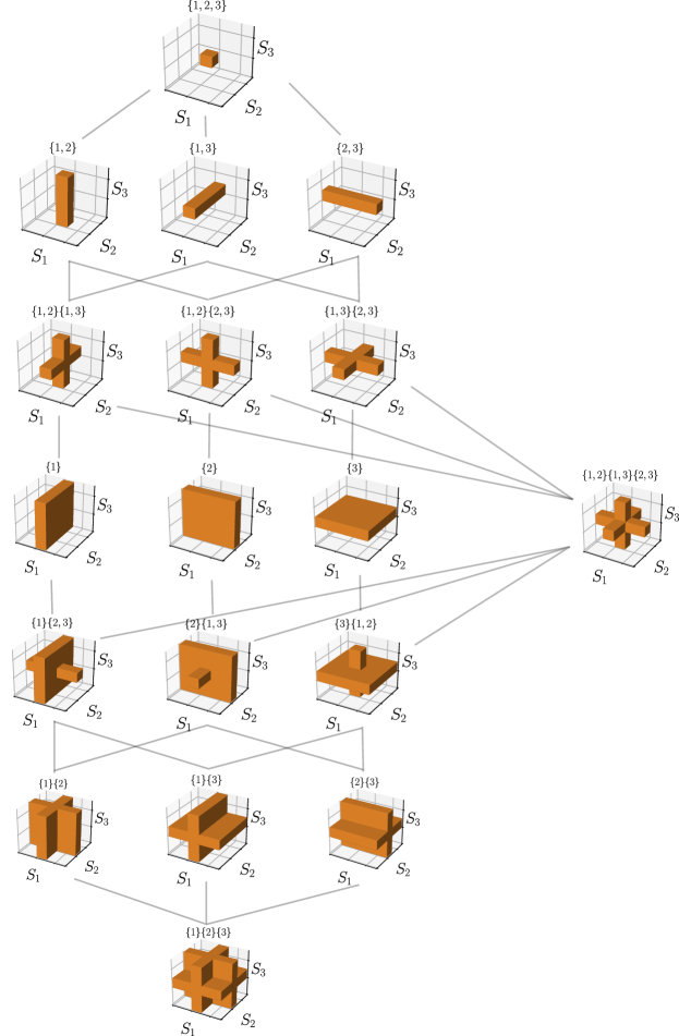
Figure 13: The nearest neighbor search regions for three source variables are cumulative when going from the full synergy (top) towards the full redundancy (bottom) in the redundancy lattice. The orange regions depict where to search for nearest neighbors, and its border signifies the surfaces of equal distance from the logical statement corresponding to each antichain. Here the finite heights, widths and depths $\epsilon$ are chosen equally large. Also note that the search regions for all classical mutual information terms (i.e., antichains $\{1,2,3\}$, $\{1,2\}$, $\{1,3\}$, $\{2,3\}$, $\{1\}$, $\{2\}$ and $\{3\}$) correspond to marginalized hypercubes, just as in the regular definition of the KSG estimator [35].

For illustration, the search regions for three source variables (trivariate PID) are visualized in Figure 13 for all antichains in the redundancy lattice.

Using this notion of neighborhood, the estimator for continuous $I^{\mathrm{sx}}_{\cap}$ can be generalized to arbitrary antichains $\alpha$ as in Definition 3, yielding

$$\begin{gathered}\hat{I}^{sx}_{\cap}(T:\alpha)\\ =\langle\widehat{\log[f^{i}_{\alpha,T}(t,s_{k})]}\rangle_{i}-\langle\widehat{\log[f^{i}_{\alpha}(s_{k})]}\rangle_{i}-\langle\widehat{\log[f^{i}_{T}(t)]}\rangle_{i}\\ =\psi(k)+\psi(N)-\langle\psi(n_{\alpha}(i))\rangle_{i}-\langle\psi(n_{T}(i))\rangle_{i}\,.\end{gathered}$$

IV Application of continuous $I^{\mathrm{sx}}_{\cap}$ estimator to simulated data from an energy management system

IV.1 Simulation of an energy management system

Figure 7: Causal structure of the energy management system model. An arrow from A to B reads as “A influences B”. Energy management system model overview: The model simulates the building power and heat demand based on time and weather conditions. Energy is provided by the grid connection, a PV-system, a combined heat and power plant (CHP), a wind turbine, and a stationary battery. The battery’s charging and discharging behavior is controlled depending on the overall power consumption level. The CHP produces energy depending on the overall power consumption and the ambient temperature.

To demonstrate the applicability of the proposed definition for continuous $I^{\mathrm{sx}}_{\cap}$ and its corresponding estimator, we applied it to simulated data for an energy management system and show how the simulated relationships between system components can be recovered from the estimated PID. In a hybrid simulation approach, we integrated real-world sensor readings from a Honda R&D facility into simulation components, which were in turn modelled via fundamental physical differential equations [41]. We informed our simulation by recordings of the actual facility energy consumption profile and local weather patterns, obtained by smart meter measurements. The simulations have been done in the Modelica simulation language, using the commercial tool SimulationX [42].

The simulation comprises multiple different agents representing energy sources, energy storage, consumers and grid interconnections. The energy originates from four sources: An on-premise wind turbine, a photovoltaic (PV) system, a combined heat and power natural gas plant (CHP), as well as energy transfers from the electricity grid. This energy is utilized as building power consumption, while excess power is stored in the battery storage system or fed back into the external power grid (see Figure 7).

In the simulation, the different agents of the system are given set rules for how they respond to each other or to external changes. Firstly, as the CHP not only provides electrical energy to the facility but also heating, it is set to operate only during times in which the ambient temperature is equal to or lower than $16\text{\,}\mathrm{\SIUnitSymbolCelsius}$. During those times, the plant produces a continuous electric power output depending on the overall energy consumption of the facility (see Algorithm 1). The stationary battery is either charged or discharged depending on the overall power consumption level of the facility (see Algorithm 2). Specifically, the storage system is set to Discharge according to a binary hysteresis with respective threshold values of $330\text{\,}\mathrm{k}\mathrm{W}$ and $350\text{\,}\mathrm{k}\mathrm{W}$ for the overall power consumption (see Figure 8). The model was simulated for a full year to capture seasonal variations in both renewable energy availability and power demand.

if $\mathrm{Temperature}\leq$16\text{\,}\mathrm{\SIUnitSymbolCelsius}$$ then

       $\mathrm{PowerOutput}\leftarrow 0.4\;\mathrm{PowerReference}$

else

       $\mathrm{PowerOutput}\leftarrow 0$

end if

Algorithm 1 CHP controller

if $\mathrm{Discharge}$ then

       $\mathrm{PowerOutput}\leftarrow-200\,000$

else if $\mathrm{PowerReference}\leq 200\,000$ then

       $\mathrm{PowerOutput}\leftarrow 100\,000$

else

       $\mathrm{PowerOutput}\leftarrow 100\,000$

end if

Algorithm 2 Battery controller

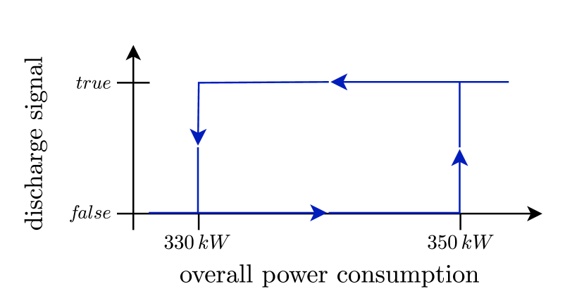
Figure 8: Hysteresis function of the battery controller: Depending on the overall power consumption level $u$, a discharge signal $y$ is sent to the controller.

The goal of the PID analysis is to find the environmental variables which best predict the total energy consumption. Specifically, we performed analyses between the total energy consumption as the target variable and used the ambient temperature, $T_{\mathrm{A}}$, wind speed, $v_{\mathrm{Wind}}$, and time of day, $t_{\mathrm{Day}}$, as sources. A full PID between these three source variables can reveal how the predictive capabilities of the environmental variables is distributed among the individual factors.

IV.2 Results of experiments

Table 2: Most information that the ambient temperature ($S_{1}=T_{A}$) and the wind speed ($S_{2}=v_{\mathrm{Wind}}$) hold about the total energy consumption ($T$) is held synergistically. The PID is calculated considering the target variable to be the total energy consumption, that is, the sum of energy consumption of the Lab and the Office building. The estimator was applied to $N=10^{5}$ data points.

	Information atom
$\Pi_{\mathrm{syn}}$	$1.735\,\mathrm{bits}$
$\Pi_{\mathrm{unq},1}$	$0.427\,\mathrm{bits}$
$\Pi_{\mathrm{unq},2}$	$0.001\,\mathrm{bits}$
$\Pi_{\mathrm{red}}$	$0.472\,\mathrm{bits}$
$I(T:S_{1},S_{2})$	$2.635\,\mathrm{bits}$

IV.2.1 Bivariate PID results

As a first step, we analyzed how well the total energy consumption is predictable from the ambient temperature $T_{A}$ and the wind speed $v_{\mathrm{Wind}}$. The results of this bivariate PID are summarized in Table 2. In total, $2.635\,\mathrm{bits}$ of information about the total energy consumption can be obtained by observing $T_{A}$ and $v_{\mathrm{Wind}}$. Intuitively, if all values for the energy consumption were equally likely, one bit of information would be equivalent to restricting the range of possible values for the energy by half after observation of the environmental variables. Accordingly, the observed $2.635\,\mathrm{bits}$ would then equate to a reduction of range of the possible outcomes by a factor of $1/6.212$.

Most of this information, namely $1.735\,\mathrm{bits}$ are carried synergistically between the two environmental variables, meaning that this information is not accessible from any individual source alone. Some of the information can also be uniquely determined from the ambient temperature ($\Pi_{\mathrm{unq},1}=0.427\,\mathrm{bits}$) and redundantly from both sources ($\Pi_{\mathrm{red}}=0.472\,\mathrm{bits}$), while the wind speed conveys hardly any information exclusively by itself ($\Pi_{\mathrm{unq},2}=0.001\,\mathrm{bits}$).

IV.2.2 Trivariate PID results

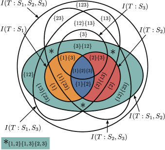
Figure 9: By adding a third source variable $S_{3}$, the four PID atoms between the target $T$ and the sources $S_{1}$ and $S_{2}$ of Figure 1 are further subdivided and new ones are added, resulting in a total of $16$ atoms [4]. The individual atoms are identified by their antichains, e.g., $\{1\}\{2,3\}$ is the redundancy between source $S_{1}$ taken alone and sources $S_{2}$ and $S_{3}$ synergistically taken together.

A possible common cause for the correlation between the environmental variables and the total energy consumption might be the time of day. To investigate this hypothesis, we augmented our analysis by incorporating the time of day as a third source variable in our PID analysis. By adding a third variable, the bivariate PID atoms themselves are dissected into smaller parts depending on their relation with the third variable (see Figure 9). For instance, the bivariate synergy $\Pi_{\mathrm{syn}}$ splits into five parts upon the introduction of the third variable, which are each characterized by a different antichain $\alpha$:

• The part of the synergy between only the sources $S_{1}$ and $S_{2}$ which is not part of $S_{3}$ ($\alpha=\{1,2\}$),

• the part of the synergy between $S_{1}$ and $S_{2}$ which is redundant with $S_{3}$ ($\alpha=\{1,2\}\{3\}$),

• the part of the synergy between $S_{1}$ and $S_{2}$ which is redundant with the synergy between $S_{1}$ and $S_{3}$ ($\alpha=\{1,2\}\{1,3\}$),

• the part of the synergy between $S_{1}$ and $S_{2}$ which is redundant with the synergy between $S_{2}$ and $S_{3}$ ($\alpha=\{1,2\}\{2,3\}$) and finally

• the part of the synergy between $S_{1}$ and $S_{2}$ which is redundant with both the synergy between $S_{1}$ and $S_{3}$ and the synergy between $S_{2}$ and $S_{3}$ ($\alpha=\{1,2\}\{1,3\}\{2,3\}$).

Table 3: The three source PID for $S_{1}=T_{\mathrm{A}},S_{2}=v_{\mathrm{Wind}}$, and $S_{3}=t_{\mathrm{Day}}$ and the total energy consumption as target variable reveals that most information that the sources carry about the target is redundant with the time of day. We list the individual 3 sources PID atoms as well as the estimated information carried by each atom $\widehat{\Pi}(T:\alpha)$ and the cumulative atoms, i.e., the corresponding estimated redundant information $\widehat{I^{\mathrm{sx}}_{\cap}}(T:\alpha)$ corresponding to the respective antichains. The estimator was applied to the same $N=100\,000$ data points as above. The total mutual information is $I(T:S_{1},S_{2},S_{3})=2.723$ bits, agreeing with the top-most redundancy in the lattice.

Parthood distribution									Estimation results
$I(T:S_{1})$	$I(T:S_{2})$	$I(T:S_{3})$	$I(T:S_{1},S_{2})$	$I(T:S_{1},S_{3})$	$I(T:S_{2},S_{3})$	$I(T:S_{1},S_{2},S_{3})$	Antichain $\alpha$	Bivariate atom	$\widehat{\Pi}(T:\alpha)$	$\widehat{I^{\mathrm{sx}}_{\cap}}(T:\alpha)$
✗	✗	✗	✗	✗	✗	✓	$\{1,2,3\}$	-	$0.421\,\mathrm{bits}$	$2.723\,\mathrm{bits}$
✗	✗	✗	✗	✓	✗	✓	$\{1,3\}$	-	$0.681\,\mathrm{bits}$	$2.169\,\mathrm{bits}$
✗	✗	✗	✗	✗	✓	✓	$\{2,3\}$	-	$0.125\,\mathrm{bits}$	$1.606\,\mathrm{bits}$
✗	✗	✗	✗	✓	✓	✓	$\{1,3\}\{2,3\}$	-	$-0.095\,\mathrm{bits}$	$1.473\,\mathrm{bits}$
✗	✗	✓	✗	✓	✓	✓	$\{3\}$	-	$-1.044\,\mathrm{bits}$	$1.083\,\mathrm{bits}$
✗	✗	✗	✓	✗	✗	✓	$\{1,2\}$	$\Pi_{\mathrm{syn}}$	$0.000\,\mathrm{bits}$	$2.635\,\mathrm{bits}$
✗	✗	✗	✓	✓	✗	✓	$\{1,2\}\{1,3\}$	$\Pi_{\mathrm{syn}}$	$0.018\,\mathrm{bits}$	$2.627\,\mathrm{bits}$
✗	✗	✗	✓	✗	✓	✓	$\{1,2\}\{2,3\}$	$\Pi_{\mathrm{syn}}$	$0.009\,\mathrm{bits}$	$2.620\,\mathrm{bits}$
✗	✗	✓	✓	✓	✓	✓	$\{3\}\{1,2\}$	$\Pi_{\mathrm{syn}}$	$1.239\,\mathrm{bits}$	$2.127\,\mathrm{bits}$
✗	✗	✗	✓	✓	✓	✓	$\{1,2\}\{1,3\}\{2,3\}$	$\Pi_{\mathrm{syn}}$	$0.469\,\mathrm{bits}$	$2.612\,\mathrm{bits}$
✓	✗	✗	✓	✓	✗	✓	$\{1\}$	$\Pi_{\mathrm{unq},1}$	$-0.003\,\mathrm{bits}$	$0.899\,\mathrm{bits}$
✓	✗	✗	✓	✓	✓	✓	$\{1\}\{2,3\}$	$\Pi_{\mathrm{unq},1}$	$0.027\,\mathrm{bits}$	$0.902\,\mathrm{bits}$
✓	✗	✓	✓	✓	✓	✓	$\{1\}\{3\}$	$\Pi_{\mathrm{unq},1}$	$0.403\,\mathrm{bits}$	$0.889\,\mathrm{bits}$
✗	✓	✗	✓	✗	✓	✓	$\{2\}$	$\Pi_{\mathrm{unq},2}$	$-0.001\,\mathrm{bits}$	$0.473\,\mathrm{bits}$
✗	✓	✗	✓	✓	✓	✓	$\{2\}\{1,3\}$	$\Pi_{\mathrm{unq},2}$	$0.003\,\mathrm{bits}$	$0.474\,\mathrm{bits}$
✗	✓	✓	✓	✓	✓	✓	$\{2\}\{3\}$	$\Pi_{\mathrm{unq},2}$	$-0.001\,\mathrm{bits}$	$0.485\,\mathrm{bits}$
✓	✓	✗	✓	✓	✓	✓	$\{1\}\{2\}$	$\Pi_{\mathrm{red}}$	$-0.014\,\mathrm{bits}$	$0.472\,\mathrm{bits}$
✓	✓	✓	✓	✓	✓	✓	$\{1\}\{2\}\{3\}$	$\Pi_{\mathrm{red}}$	$0.486\,\mathrm{bits}$	$0.486\,\mathrm{bits}$

Examining the estimation results of the trivariate PID, as listed in Table 3 and visualized in Figure 10, we can observe that the synergy between ambient temperature and wind speed primarily resides within the trivariate atom characterized by the antichain $\{1,2\}\{3\}$. This implies that the bivariate synergy between $T_{A}$ and $v_{\mathrm{Wind}}$ largely duplicates the information conveyed by the time of day. A similar trend emerges when considering bivariate redundancy $\Pi_{\mathrm{red}}$, which also predominantly overlaps with the time of day, i.e., resides mainly in the trivariate atom $\{1\}\{2\}\{3\}$, and also the bivariate unique information of the ambient temperature $\Pi_{\mathrm{unq},1}$, which mostly resides in the redundant atom $\{1\}\{3\}$. These findings substantiate our hypothesis that weather variables primarily act as intermediaries, conveying information that the time of day carries about the energy consumption.

Nevertheless, there are also other PID atoms which contribute non-negligibly to the total mutual information. In particular, some information is carried synergistically between the ambient temperature and the time of day ($\{1,3\}$) or, to a lesser extent, between the synergy between all variables ($\{1,2,3\}$) and the synergy between wind speed and the time of day ($\{2,3\}$). Yet other relevant contributions come from the redundancy between the ambient temperature and the time of day ($\{1\}\{3\}$) and the redundancy between all three two-variable synergies ($\{1,2\}\{1,3\}\{2,3\}$).

Finally, note that the information that the time of day provides uniquely and independent of ambient temperature and wind speed is on average negative, i.e., misinformative about the total power draw. Average misinformation can arise in $I^{\mathrm{sx}}_{\cap}$ since the operational interpretation, which has been put forward in Makkeh et al. [26] and carries over to the continuous case, assumes a memoryless agent and interprets the average information-theoretic quantities as ensemble averages. For a hypothetical agent incapable of learning from past events, this means that gaining only the purely unique information of the time of day diminishes the agent’s accuracy in predicting the total power draw.

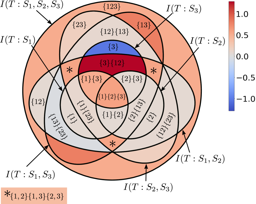
Figure 10: Visually, the fact that much of the information in sources $S_{1}$ (ambient temperature) and $S_{2}$ (wind speed) is redundant with $S_{3}$ (time of day) is apparent from the fact that many of the most informative atoms (red) are contained within the circle of $I(T:S_{3})$. This diagram visualizes the results of Table 3. Here, red encodes positive, i.e., net informative, information contributions carried by the associated information atom, while blue encodes negative, i.e., net misinformative contributions.

V Discussion

This work presents a tractable analytical definition of continuous PID which is based on the intuitive ideas of the discrete $I^{\mathrm{sx}}_{\cap}$ measure [26] and the measure-theoretical existence proofs by Schick-Poland et al. [34]. It is in a local form by definition, is applicable to arbitrary many source variables and differentiable. We exemplify the intuition of our definition on four toy examples and observe that the measure gives mostly qualitatively comparable results to the the discrete case when computed on continuous versions of certain logic gates. Furthermore, we provide a nearest-neighbor based estimator and show that it converges to the numerically obtained values on the before-mentioned examples. Lastly, we demonstrate how this estimator can be used in a practical example by using it to uncover variable dependencies in a simulated energy management system.

As outlined in Section II.2, the definition of continuous $I^{\mathrm{sx}}_{\cap}$ leaves open a choice of how to set the relative scale between variables that needs to be made in accordance with the setup in question. While such a choice marks a departure from the purely model-free nature of classical information theory, note that this is likely unavoidable in a PID context. For PID itself, choosing one of the multiple competing PID measures according to their operational interpretation similarly introduces some notion of “proto-semantics” to the analysis. Overall, we see the choice of relative scale not as a weakness but as a necessity for a continuous PID measure, since what it means to be in a neighborhood of a value might differ drastically between different variables.

This work builds on the definition of the discrete $I^{\mathrm{sx}}_{\cap}$ measure [26] and its measure-theoretic extension to continuous variables [34] to introduce a tractable analytical definition and practical nearest-neighbor based estimator for a continuous $I^{\mathrm{sx}}_{\cap}$ measure. However, this definition turns out not to be invariant with respect to bijective transformations of the individual variables–at least not without prescribing a preprocessing scheme (see Appendix G). Yet, this invariance is a property central to the measure-theoretic derivation in [34]. For this reason, the analytic definition presented here cannot be directly interpreted as a concretization of the latter but should rather be seen as a practical implementation rooted in the intuitive meaning of the $I^{\mathrm{sx}}_{\cap}$ measure.

Like in the discrete case, this definition of redundancy might yield negative information atoms. In the context originally introduced by Makkeh et al. [26], namely for memory-less agents and interpreting the average in Equation 5 as an ensemble average, these are easily interpreted as misinforming the agents of the ensemble on average. For time-series data, for which the averages are taken over time, however, negative atoms can be a distracting technicality hindering a straightforward interpretation of the results. In these cases, practitioners may opt to clamp the atoms to non-negative values and adjust the other atoms accordingly so that the consistency equations (Equations (15) for the general case) continue to hold.

In this paper, we propose a novel shared-exclusion based PID measure designed specifically for purely continuous variables. However, it is important to acknowledge that real-world systems often involve a combination of continuous and discrete source variables. Additionally, even certain individual variables may comprise both discrete and continuous parts. To address these scenarios, we introduce an analytical formulation in Appendix J, outlining an ansatz for handling mixed systems. While we defer the presentation of specific examples demonstrating its application and the development of a mixed continuous-discrete estimator to future research, this work lays the groundwork for a comprehensive understanding of information decomposition in systems with diverse variable types.

Overall, with this paper we introduce a new analytical formulation for a shared-exclusion based continuous PID measure and provide an estimator that makes it applicable to practitioners from all sciences and technology.

Appendix A On the shared-exclusions measure of redundancy

The definition of bivariate $I^{\mathrm{sx}}_{\cap}$ in Definition 2 can also be derived from shared exclusions of parts of the underlying probability space, i.e., the parts of the probability space that are rendered impossible by observation of either variable. To determine the precise subsets of the probability space to be excluded, we assume that a realization $\bm{S}=(S_{1},S_{2})=\bm{s}=(s_{1},s_{2})$ has been taken by the system and we have gained the information that either $S_{1}=s_{1}$ or $S_{2}=s_{2}$ have materialized. Through this observation, the part of the probability space corresponding to any other realization $\bm{s}^{\prime}=(s_{1}^{\prime},s_{2}^{\prime})$ is rendered impossible unless either $s_{1}^{\prime}=s_{1}$ or $s_{2}^{\prime}=s_{2}$. If neither of those equations holds, then $\bm{s}^{\prime}$ would not fulfill the logical or-statement in Definition 2 and would hence be impossible under the assumption (see Figure 11).

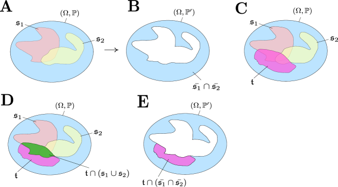
Figure 11: The pointwise redundancy $i^{\mathrm{sx}}_{\cap}$ can be derived from principles of probability exclusion. Local redundant information for two sources $S_{1}$ and $S_{2}$ with respect to target $T$ at a joint realization $(s_{1},s_{2},t)$. Each realization corresponds to one of the events in the probability space denoted by $\mathfrak{s}_{1},\mathfrak{s}_{2}$ and $\mathfrak{t}$ in the probability space $(\Omega,\mathbb{P})$. Here we aim at assessing the benefit of knowing that either $S_{1}=s_{1}$ or $S_{2}=s_{2}$ in predicting $t$. In panel $\mathbf{A}$ the events $\mathfrak{s}_{1}$ and $\mathfrak{s}_{2}$ are displayed. In panel $\mathbf{B}$ there is the intersection of both complements from the events in panel $\mathbf{A}$, which is the area of probability mass which either event excludes. In panel $\mathbf{C}$ we consider a target variable and its event set $\mathfrak{t}$ in $\Omega$, while panel D shows the area of interest, the green set represents the part of event $\mathfrak{t}$ that is included in also either $\mathfrak{s}_{1}$ or in $\mathfrak{s}_{2}$ which corresponds to the part of the probability of realization $t$, which is accessible when assuming that the logical statement $S_{1}=s_{1}\lor S_{2}=s_{2}$ is true, or, correspondingly, $W_{\{1\},\{2\}}=1$. While the green area can be measured via the probability measure directly, i.e., $\mathbb{P}(\mathfrak{t}\cap(\mathfrak{s}_{1}\cup\mathfrak{s}_{2}))$, we can similarly represent it using the shared exclusion overlapping with $\mathfrak{t}$ as in panel $\mathbf{E}$, by $\mathbb{P}^{\prime}(\mathfrak{t})-\mathbb{P}^{\prime}(\mathfrak{t}\cap(\bar{\mathfrak{s}_{1}}\cap\bar{\mathfrak{s}_{2}}))=\frac{\mathbb{P}(\mathfrak{t})-\mathbb{P}(\mathfrak{t}\cap(\bar{\mathfrak{s}_{1}}\cap\bar{\mathfrak{s}_{2}}))}{1-\mathbb{P}(\mathfrak{s}_{1}\cup\mathfrak{s}_{2})}$. This green area then has to be compared to the regular probability of obtaining the realization $t$ without knowledge of any of the sources, $\mathbb{P}(\mathfrak{t})$.

When parts of the probability space are rendered impossible by observing a certain event, the resulting posterior probability measure $\mathbb{P}$ needs to be normalized on $\Omega$, yielding an adapted probability measure $\mathbb{P}^{\prime}$, known as the conditional probability measure. The visualization Figure 11 shows the exclusion of specific parts of the probability space leading to descriptions of the information that can be assessed from either $S_{1}$ or $S_{2}$ locally about $T$.

Similarly, this concept can then be generalized to collections $\alpha=\{\bm{a}_{j}\}_{j}=\{\{s_{ij}\}_{i}\}_{j}$ of three or more source variables by excluding the part of the probability space that is redundantly excluded by all joint collections of random variables $a_{j}$. For instance, in a quadrivariate (i.e., four source variable) system, the redundancy between the collections $\{S_{1},S_{3}\}$ and $\{S_{2},S_{4}\}$ is defined by the joint exclusions between the collections, which is given by all realizations $\bm{s}^{\prime}=(s^{\prime}_{1},s^{\prime}_{2},s^{\prime}_{3},s^{\prime}_{4})$ for which neither $(s^{\prime}_{1},s^{\prime}_{3})=(s_{1},s_{3})$ nor $(s^{\prime}_{2},s^{\prime}_{4})=(s_{2},s_{4})$ holds. This generalization to collections of subsets of the source variables turns out to be of the form of local mutual information with respect to an auxiliary random variable

$$\mathcal{W}_{\Phi}(\bm{s})=\bigvee\limits_{a\in\mathcal{P}(\mathbf{S}):\Phi(a)=1}\bigwedge\limits_{i\in a}(S_{i}=s_{i})$$

and reverts to a classical mutual information quantity for self-redundancies, i.e., $\alpha=\{\bm{a}\}$. Further, its dependence on elements of the power set of the index set of sources (set of all collections of sources) implies that the $I^{\mathrm{sx}}_{\cap}$ measure of redundant information gives rise to a full lattice of PID atoms as described in Section III.1. Note also that this measure, as a composition of differentiable functions, is differentiable itself with respect to minor perturbations of the underlying probability mass function. Additionally, it fulfills a target chain rule.

Appendix B Proof of the differentiability of $I^{\mathrm{sx}}_{\cap}$

The analytical definition of the redundancy (see Definition 2) allows us to prove its differentiability and even smoothness for both the local and global measure.

Theorem 1.

The local continuous measure of shared information

$$i^{\mathrm{sx}}_{\cap}[f](t,\{s_{1}\}\{s_{2}\}) =\log_{2}\left[\frac{f_{T|S_{1}\lor S_{2}}(t|s_{1}\lor s_{2})}{f_{T}(t)}\right]$$

$$=\log_{2}\left[\frac{f_{TS_{1}}(t,s_{1})+f_{TS_{2}}(t,s_{2})}{f_{T}(t)(f_{S_{1}}(s_{1})+f_{S_{2}}(s_{2}))}\right]$$

varies smoothly with respect to changes of the underlying joint probability density $f_{TS_{1}S_{2}}$. Moreover, for more than two source variables, $i_{\cap}^{\mathrm{sx}}[f_{TS_{1}S_{2}}](t:\alpha)$ is smooth for arbitrary antichains $\alpha$.

Proof.

Let $f_{TS_{1}S_{2}}$ be a density function and $(t,s_{1},s_{2})$ a point in state space such that $f_{TS_{1}S_{2}}(t,s_{1},s_{2})>0$. Now, let $g_{TS_{1}S_{2}}$ be a function such that $g_{TS_{1}S_{2}}(t,s_{1},s_{2})\neq 0$.

Then we construct the derivative $D(i_{\cap}^{\mathrm{sx}}[f])g$ in the direction of $g$ by considering the limit of a shifted density $f_{TS_{1}S_{2}}\mapsto f_{TS_{1}S_{2}}+\epsilon\cdot g_{TS_{1}S_{2}}$ with $\epsilon>0$, yielding

$$D(i_{\cap}^{\mathrm{sx}}[f])g= \lim_{\epsilon\to 0}\frac{i_{\cap}^{\mathrm{sx}}[f_{TS_{1}S_{2}}+\epsilon\cdot g_{TS_{1}S_{2}}](t:s_{1}\lor s_{2})-i_{\cap}^{\mathrm{sx}}[f_{TS_{1}S_{2}}](t:s_{1}\lor s_{2})}{\epsilon}$$

$$= \lim_{\epsilon\to 0}\frac{\log\left[\frac{f_{TS_{1}}(t,s_{1})+f_{TS_{2}}(t,s_{2})+\epsilon(g_{TS_{1}}(t,s_{1})+g_{TS_{2}}(t,s_{2}))}{(f_{T}(t)+\epsilon g_{T}(t))(f_{S_{1}}(s_{1})+f_{S_{2}}(s_{2})+\epsilon(g_{S_{1}}(s_{1})+g_{S_{2}}(s_{2}))}\right]-\log\left[\frac{f_{TS_{1}}(t,s_{1})+f_{TS_{2}}(t,s_{2})}{f_{T}(t)(f_{S_{1}}(s_{1})+f_{S_{2}}(s_{2}))}\right]}{\epsilon}$$

$$= \lim_{\epsilon\to 0}\frac{\log_{2}\left[1+\epsilon\frac{g_{TS_{1}}(t,s_{1})+g_{TS2}(t,s_{2})}{f_{TS_{1}}(t,s_{1})+f_{TS_{2}}(t,s_{2})}\right]-\log_{2}\left[1+\epsilon\frac{g_{S_{1}}(s_{1})+g_{S_{2}}(s_{2})}{f_{S_{1}}(s_{1})+f_{S_{2}}(s_{2})}\right]-\log_{2}\left[1+\epsilon\frac{g_{T}(t)}{f_{T}(t)}\right]}{\epsilon}\,.$$

At this point, we use the Taylor expansion $\ln[1+x]=\sum\limits_{n=1}^{\infty}\frac{(-1)^{n+1}x^{n}}{n}=x+\mathcal{O}(x^{2})$ to determine the final form of the derivative

$$D(i_{\cap}^{\mathrm{sx}}[f])g =\frac{g_{TS_{1}}(t,s_{1})+g_{TS_{2}}(t,s_{2})}{f_{TS_{1}}(t,s_{1})+f_{TS_{2}}(t,s_{2})}-\frac{g_{S_{1}}(s_{1})+g_{S_{2}}(s_{2})}{f_{S_{1}}(s_{1})+f_{S_{2}}(s_{2})}-\frac{g_{T}(t)}{f_{T}(t)}\,,$$

which is finite by assumption.

Considering the form that results from the derivative, it can be concluded that the $i_{\cap}^{\mathrm{sx}}[f_{TS_{1}S_{2}}](t:s_{1}\lor s_{2})$ is not only differentiable at point $(t,s_{1},s_{2})$, but even smooth, since the following derivatives will be linear combinations of powers of terms of the form $\frac{1}{f_{TS_{1}}+f_{TS_{2}}}$, $\frac{1}{f_{S_{1}}+f_{S_{2}}}$ and $\frac{1}{f_{T}}$.

Note further that this proof naturally extends to any arbitrary antichain $\alpha$ of interest by an analogous argument. ∎

Corollary 1.

The global measure of redundant information $I^{\mathrm{sx}}_{\cap}[f]=\int f\,i^{\mathrm{sx}}_{\cap}[f]$ is a smooth functional of the underlying density $f$ if $f$ and its marginals are bounded from below by some $\xi>0$.

Proof.

The change of $I^{\mathrm{sx}}_{\cap}$ when shifting $f$ infinitesimally in the direction of $g$ is given by

$$\left[\frac{\mathrm{d}I^{\mathrm{sx}}_{\cap}[f+\epsilon g]}{\mathrm{d}\epsilon}\right]_{\epsilon=0}=\int\mathrm{d}t\mathrm{d}s_{1}\mathrm{d}s_{2}\,\frac{\delta I^{\mathrm{sx}}_{\cap}[f]}{\delta f(t,s_{1},s_{2})}g(t,s_{1},s_{2})\,.$$

where $\delta I^{\mathrm{sx}}_{\cap}[f]/\delta f(t,s_{1},s_{2})$ is the functional derivative of $I^{\mathrm{sx}}_{\cap}$ [43]. By applying a product rule of differentiation to the functional

$$I^{\mathrm{sx}}_{\cap}[f]=\int\mathrm{d}t\,\mathrm{d}s_{1}\,\mathrm{d}s_{2}\,f(t,s_{1},s_{2})\,i^{\mathrm{sx}}_{\cap}[f](t,s_{1},s_{2})\,,$$

which depends on $f$ in two places, we obtain

$$\left[\frac{\mathrm{d}I^{\mathrm{sx}}_{\cap}[f+\epsilon g]}{\mathrm{d}\epsilon}\right]_{\epsilon=0}$$

$$=\left[\frac{\mathrm{d}}{\mathrm{d}\epsilon}\int\mathrm{d}t\,\mathrm{d}s_{1}\,\mathrm{d}s_{2}\,(f+\epsilon g)(t,s_{1},s_{2})\right.$$

$$\left.\vphantom{\int}i^{\mathrm{sx}}_{\cap}[f+\epsilon g](t,s_{1},s_{2})\right]_{\epsilon=0}$$

$$=\int\mathrm{d}t\mathrm{d}s_{1}\mathrm{d}s_{2}\,\{i^{\mathrm{sx}}_{\cap}[f](t,s_{1},s_{2})\,g(t,s_{1},s_{2})$$

$$+f(t,s_{1},s_{2})\left[D(i^{\mathrm{sx}}_{\cap}[f])g\right](t,s_{1},s_{2})\}$$

$$=\int\mathrm{d}t\mathrm{d}s_{1}\mathrm{d}s_{2}\,\left[\left\{i^{\mathrm{sx}}_{\cap}[f]+fD(i^{\mathrm{sx}}_{\cap}[f])\right\}g\right](t,s_{1},s_{2})\,,$$

from which we can read off the functional derivative as the functional

$$\frac{\delta I^{\mathrm{sx}}_{\cap}[f]}{\delta f(t,s_{1},s_{2})}=i^{\mathrm{sx}}_{\cap}[f]+fD(i^{\mathrm{sx}}_{\cap}[f])\,.$$

If the marginals of the joint density $f$ are bounded from below, the magnitude of the Fréchet derivative, $|D_{g}(i_{\cap}^{\mathrm{sx}}[f])|$, is bounded, too. Hence the functional derivative is well-defined for all points $(t,s_{1},s_{2})$. Thus the total change of the functional $I^{\mathrm{sx}}_{\cap}[f]$ with respect to an infinitesimal change of $f$ in the direction of $g$ exists if and only if both $i^{\mathrm{sx}}_{\cap}[f]g$ and $fD(i^{\mathrm{sx}}_{\cap}[f])g$ are integrable functions over the space of realizations. ∎

Appendix C Analytical probability distributions for the logic gates and sum examples

The probability densities for the three continuous logic gates as well as the sum example can be expressed as multivariate Gaussian distributions of the form

$$p_{T,S_{1},S_{2}}(t,s_{1},s_{2})=\frac{1}{\sqrt{(2\pi)^{l}\det\Sigma}}\exp{-\frac{1}{2}\bm{x}^{T}\,\Sigma^{-1}\,\bm{x}}\,,$$

where $\bm{x}=\begin{pmatrix}t&s_{1}&s_{2}\end{pmatrix}^{T}$ and the covariance matrix $\Sigma$ depends on the gate. Note, further, that the integer $l$ is equal to $3$ for the redundant and unique gate as well as the sum example while it is equal to $4$ for the copy gate because of the two-dimensional target.

To make the mutual information finite, noise with standard deviation $\sigma=0.01$ is added to the target variable. Furthermore, an auxiliary variable $\delta=10^{-8}$ is introduced in the redundant gate for numerical reasons to avoid a singular matrix.

The covariance matrices are found as follows:

Redundant gate

$$\Sigma=\begin{pmatrix}1+\sigma^{2}&1-\delta&1-\delta\\ 1-\delta&1&1-\delta\\ 1-\delta&1-\delta&1\end{pmatrix}$$

Copy gate

$$\Sigma=\begin{pmatrix}1+\sigma^{2}&0&1&0\\ 0&1+\sigma^{2}&0&1\\ 1&0&1&0\\ 0&1&0&1\end{pmatrix}$$

where $l=4$ and $\bm{x}=\begin{pmatrix}t_{1},t_{2},s_{1},s_{2}\end{pmatrix}^{T}$)

Unique gate

$$\Sigma=\begin{pmatrix}1+\sigma^{2}&1&0\\ 0&1&0\\ 1&0&1\\ \end{pmatrix}$$

Continuous sum

$$\Sigma=\begin{pmatrix}2+\sigma^{2}&1&1\\ 1&1&0\\ 1&0&1\end{pmatrix}\,.$$

Appendix D Formal Derivation of the Kozachenko-Leonenko Estimator for Shannon Differential Entropy

The proposed estimator for continuous $I^{\mathrm{sx}}_{\cap}$ is based on ideas of the KSG estimator, originally introduced by Kraskov et al. [35] in 2004, which is explained here for completeness. The main advancement of the KSG estimator was to apply the Kosachenko-Leonenko estimator [39] for (differential) entropy in a specific way, allowing for estimation of $I(X;Y)=H(X)+H(Y)-H(X,Y)$. Here we will continue in a very similar fashion.

Kosachenko and Leonenko estimate (differential) entropy on the grounds of the assumption that the density to consider for the entropy is locally constant around a measured data point $x_{i}$, i.e., $q_{i}(\epsilon)=\int\limits_{B_{\epsilon}(x_{i})}\mathrm{d}x\,p_{X}(x)\approx\lambda_{X}\left(B_{\epsilon}(x_{i})\right)p_{X}(x_{i})$, where $B_{\epsilon}(x_{i})$ is the $\epsilon$-ball around $x_{i}$. Then Kosachenko and Leonenko introduce a probability density function $P_{k}(\epsilon)$, such that $P_{k}(\epsilon)d\epsilon$ determines the probability of $k-1$ points lying within radius $\epsilon$ around $x_{i}$, a $k$-th lying within the shell of radii within $[\epsilon,\epsilon+d\epsilon]$ around $x_{i}$, and the remaining $N-k-1$ points lying outside.

Using well-known integral identities, we find

$$\int\limits_{\mathbb{R}^{+}}\mathrm{d}\epsilon\,\log[q_{i}(\epsilon)]P_{k}(\epsilon)=\psi(k)-\psi(N)\,,$$

with $B(x,y)$ the beta function.

Then, since $p_{X}(x_{i})\lambda_{X}\left(B_{\epsilon_{i}}(x_{i})\right)\approx q_{i}(\epsilon_{i})$, it follows that

$$\log\left[p_{X}(x_{i})\lambda_{X}\left(B_{\epsilon_{i}}(x_{i})\right)\right]\approx\mathbb{E}\left[\log[q_{i}]\right]=\psi(k)-\psi(N)$$

such that a point estimate $\hat{H}$ of the differential entropy can be determined as

$$\hat{H}(X)=-\frac{1}{N}\sum\limits_{i=1}^{N}\widehat{\log\left[p_{X}(x_{i})\right]}$$

$$=-\psi(k)+\psi(N)+\frac{1}{N}\sum\limits_{i=1}^{N}\log\left[\lambda_{X}\left(B_{\epsilon_{i}}(x_{i})\right)\right].$$

The volume bias terms $\lambda_{X}\left(B_{\epsilon}(x_{i})\right)$ are numerically obtained by performing searches for the $k$-th nearest neighbor in the data set, the distance to whom is $\epsilon_{i}$.

Appendix E Arriving at the KSG Estimator for Mutual Information

The KSG ansatz combines three Kosachenko-Leonenko estimators in order to estimate $I(X;Y)$. It does so by, for each point, first searching the $k$-th nearest neighbor in the joint space with respect to $\max\left(\norm{\cdot}_{X},\norm{\cdot}_{Y}\right)$, to obtain $\epsilon_{i}$. Then the same $\epsilon_{i}$ is used to search the numbers of nearest neighbors, $n_{X}(i),n_{Y}(i)$, within this radius in both marginal spaces. The choice of taking the same epsilon for the subspaces ultimately cancels the volume terms $\left\langle\lambda_{j}\left(B_{\epsilon_{i}}\right)\right\rangle_{i}$ from the estimator completely as, in the maximum norm, $\lambda_{XY}(B_{\epsilon_{i}}(x_{i})\times B_{\epsilon_{i}}(y_{i}))=\lambda_{X}(B_{\epsilon_{i}}(x_{i}))\lambda_{Y}(B_{\epsilon_{i}}(y_{i}))$, yielding

$$\hat{I}(X,Y)=\psi(k)+\psi(N)-\left\langle\psi(n_{X}(x_{i}))+\psi(n_{Y}(y_{i}))\right\rangle_{i}\,.$$

Appendix F Construction of densities of logical statements

In this appendix section we argue for the explicit form of the quasi-densities appearing in $I^{\mathrm{sx}}_{\cap}$, which stem from a logical statement allowing also for disjunctions, and not only conjunctions as is usual in traditional probability theory.

Let us recall that when measuring a union of two sets, by the law of inclusion-exclusion, we can express the result as the following sum:

$$\mathbb{P}^{S_{1},S_{2}}(B\cup C)$$

$$=\mathbb{P}^{S_{1},S_{2}}(B)+\mathbb{P}^{S_{1},S_{2}}(C)-\mathbb{P}^{S_{1},S_{2}}(B\cap C)\,.$$

Similarly to Appendix A, a union can be utilized to represent the logical disjunction $S_{1}\in B\lor S_{2}\in C$ via measuring the set $B\times E_{S_{2}}\cup E_{S_{1}}\times C$ where $E_{S_{i}}$ denotes the respective space of possible realizations for $S_{i}$. Measuring $B\times E_{S_{2}}\cup E_{S_{1}}\times C$ then yields

$$\mathbb{P}^{S_{1},S_{2}}(B\times E_{S_{2}}\cup E_{S_{1}}\times C)$$

$$=\mathbb{P}^{S_{1}}(B)+\mathbb{P}^{S_{2}}(C)-\mathbb{P}^{S_{1},S_{2}}(B\cap C)\,,$$

i.e., by using the marginal measures, just as it is done in discrete settings. Suppose now that we know that the statement $S_{1}\in B\lor S_{2}\in C$ is true. How would we measure the probability of additional events under this presumption? Assuming the event $S_{1}\in B\lor S_{2}\in C$ is true means that we need to use a conditional probability measure to measure additional events $A\in E_{S_{1}}\times E_{S_{2}}$. Thus, to obtain a probability measure under the assumption that $S_{1}\in B\lor S_{2}\in C$ is true, we can write

$$\mathbb{P}^{(S_{1},S_{2})}_{S_{1}\in B\lor S_{2}\in C}(A):=\mathbb{P}^{S_{1}}(A\cap B)+\mathbb{P}^{S_{2}}(A\cap C)$$

$$-\mathbb{P}^{(S_{1},S_{2})}(A\cap(B\times C)).$$

Applying this to infinitesimally small sets $B=\{s_{1}\}$ and $C=\{s_{2}\}$, we can achieve the same form by adding slices of conditional measures with respect to the constraints set by the disjunction. We define

$$\mathbb{P}^{(S_{1},S_{2})}_{(S_{1}=s_{1})\lor(S_{2}=s_{2})}(A):=\mathbb{P}^{S_{1}}(\{x|(x,y)\in A,y=s_{2}\})$$

$$+\mathbb{P}^{S_{2}}(\{y|(x,y)\in A,x=s_{1}\})-\mathbb{P}^{(S_{1},S_{2})}(\{(s_{1},s_{2})\}\cap A)$$

for an event $A$.

Note that when taking the limit to infinitesimal sets, a choice needs to be made regarding the relative rate of convergence of the two variables. Choosing to interpret the two variables as being on equal scales, i.e., using the same $\epsilon$ to search in the respective marginal neighborhoods, this uniquely defines the measure as the only one fulfilling

$$\norm{\mathbb{P}^{(S_{1},S_{2})}_{(S_{1}\in B_{s_{1}}(\epsilon))\lor(S_{2}\in B_{s_{2}}(\epsilon))}(A)-\epsilon\cdot\mathbb{P}^{(S_{1},S_{2})}_{(S_{1}\in\{s_{1}\})\lor(S_{2}\in\{s_{2}\})}(A)}\leq C_{\epsilon}\cdot\epsilon\overset{\epsilon\searrow 0}{\to}0\quad\forall A\in\mathcal{E}\,,$$

with $C_{\epsilon}\overset{\epsilon\searrow 0}{\to}C$, where $C$ is a constant. This can easily be seen when using the triangle inequality and recalling the form of a conditional probability measure, i.e.,

$$\mathbb{P}^{S_{1},S_{2}}(\{(x,y)\in A|y\in B_{s_{2}}(\epsilon)\}) =\underbrace{\frac{\mathbb{P}^{S_{1},S_{2}}(\{(x,y)\in A|y\in B_{s_{2}}(\epsilon)\})}{\mathbb{P}^{S_{2}}(B_{s_{2}}(\epsilon))}}_{\overset{\epsilon\searrow 0}{\to}\mathbb{P}^{S_{1}}(\{(x,y)\in A|y=s_{2}\})}\underbrace{\frac{\mathbb{P}^{S_{2}}(B_{s_{2}}(\epsilon))}{\lambda_{S_{2}}(B_{s_{2}}(\epsilon))}}_{\overset{\epsilon\searrow 0}{\to}f_{S_{2}}(s_{2})}\underbrace{\lambda_{S_{2}}(B_{s_{2}}(\epsilon))}_{2\epsilon}$$

$$\quad\overset{\epsilon\ll 1}{\sim}2\epsilon\mathbb{P}^{S_{1}}(\{(x,y)\in A|y=s_{2}\})f_{S_{2}}(s_{2})\,.$$

This idea is further visualized in Figure 12.

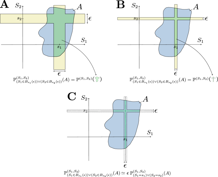
Figure 12: We choose our localized conditional probability measure such that its extension for small neighbourhoods naturally results in the global probability measure. In panel A the intuitive meaning of the measure $\mathbb{P}^{(S_{1},S_{2})}_{(S_{1}\in B_{s_{1}}(\epsilon))\lor(S_{2}\in B_{s_{2}}(\epsilon))}(A)$ for a set $A$ is illustrated. In panel B one sees the consequences of $\epsilon$ decreasing, leading to $\mathbb{P}^{(S_{1},S_{2})}_{(S_{1}\in B_{s_{1}}(\epsilon))\lor(S_{2}\in B_{s_{2}}(\epsilon))}(A)$ approaching the conditional measure of our choice, $\mathbb{P}^{(S_{1},S_{2})}_{(S_{1}\in\{s_{1}\})\lor(S_{2}\in\{s_{2}\})}(A)$ multiplied with the width of the neighborhood, $\epsilon$, as shown in panel C.

Evidently, this ansatz fails if any of the marginal densities $f_{S_{i}}$ is unbounded at $s_{i}$. The choice of this measure could also be argued for as a consequence of the simple function approximation, found for instance in [44], thrm. 7.10.

To arrive at a probability for an infinitesimal event, compare the above to the construction of the usual Lebesgue measure $\lambda_{S}$ measuring the maximal size of nicely shrinking balls $B_{i}=B_{(s_{1},s_{2})}(r_{i})$ [44]. Note that the maximal size of a $B_{i}$ is the diameter of the ball, $2r_{i}$, and in the continuous case, the last term in the numerator vanishes.

Then

$$f_{S_{1}\lor S_{2}}(s_{1},s_{2})$$

$$= \lim\limits_{B_{i}\searrow\{(s_{1},s_{2})\}}\frac{\mathbb{P}^{(S_{1},S_{2})}_{(S_{1}=s_{1})\lor(S_{2}=s_{2})}(B_{(s_{1},s_{2})}(r_{i}))}{\lambda_{S}(B_{(s_{1},s_{2})}(r_{i}))}$$

$$= \lim\limits_{r_{i}\searrow 0}\frac{\mathbb{P}^{S_{1}}(\{(x,y)\in B_{i}|y=s_{2}\})}{2r_{i}}$$

$$+\frac{\mathbb{P}^{S_{2}}(\{(x,y)\in B_{i}|x=s_{1}\})}{2r_{i}}$$

$$= \lim\limits_{r_{i}\searrow 0}\frac{\mathbb{P}^{S_{1}}(\{s_{1}\pm r_{i}\})+\mathbb{P}^{S_{2}}(\{s_{2}\pm r_{i}\})}{2r_{i}}$$

$$= f_{S_{1}}(s_{1})+f_{S_{2}}(s_{2})\,,$$

where $\lambda_{S_{1}}(\{(x,y)\in B_{i}|y=s_{2}\})+\lambda_{S_{2}}(\{(x,y)\in B_{i}|x=s_{1}\}$ is equal to $2r_{i}$ since the measures $\lambda_{S_{i}}$ measure the diameter of the uniform ball centered around $(s_{1},s_{2})$.

This method is readily generalized to $n$ sources in the exact same way it worked for two, with the one exception being that conjunctions are treated as one variable. For example, a logical statement $\alpha(s_{1},s_{2},s_{3})=\{S_{1}=s_{1}\}\land\{S_{2}=s_{2}\}\lor\{S_{3}=s_{3}\}$ is treated as a disjunction of a single two dimensional statement and a single one dimensional statement.

Definition 3.

Let for a generic logical statement $\alpha$ of length $l(\alpha)$ in its disjunctive normal form $\alpha=\bigvee_{j\in J}a_{j}$, $I_{d}\subset J$ be the subset of purely discrete statements. Then we define the density of $\alpha$ as

$$\frac{\delta\mathbb{P}_{\lor}}{\delta\lambda_{\lor}}(s_{1},\ldots s_{n})=f_{\alpha}(x_{1},\ldots x_{n}):=\sum\limits_{k=1}^{|I_{d}|+1}(-1)^{k+1}\left(\sum\limits_{\begin{subarray}{c}m_{1}<m_{2}<\ldots<m_{k-1}\in I_{d}\\ m_{1}\neq m_{2}\neq\ldots\neq m_{k-1}\neq j\in J\end{subarray}}f_{\bigcup\limits_{q=1}^{k-1}a_{m_{q}}\cup a_{j}}\left(\bigcup\limits_{q=1}^{k-1}x_{a_{m_{q}}}\cup x_{a_{j}}\right)\right)\,.$$

Table 4: Different preprocessing schemes for continuous PID gates produce qualitatively similar results on the redundant and unique gate, while a copula pretransformation results in different results for the copy and sum gates. The results have been computed using a Monte-Carlo integration analogous to Table 1.

	Redundant Gate	Copy Gate	Unique Gate	Sum
No transformation
$\Pi_{\mathrm{syn}}$	$0.000\,\mathrm{bits}$	$6.644\,\mathrm{bits}$	$5.525\,\mathrm{bits}$	$6.497\,\mathrm{bits}$
$\Pi_{\mathrm{unq,1}}$	$0.000\,\mathrm{bits}$	$0.000\,\mathrm{bits}$	$1.119\,\mathrm{bits}$	$0.147\,\mathrm{bits}$
$\Pi_{\mathrm{unq,1}}$	$0.000\,\mathrm{bits}$	$0.000\,\mathrm{bits}$	$-5.525\,\mathrm{bits}$	$0.147\,\mathrm{bits}$
$\Pi_{\mathrm{red}}$	$6.644\,\mathrm{bits}$	$6.644\,\mathrm{bits}$	$5.525\,\mathrm{bits}$	$0.353\,\mathrm{bits}$
$I(T:S_{1},S_{2})$	$6.644\,\mathrm{bits}$	$13.288\,\mathrm{bits}$	$6.644\,\mathrm{bits}$	$7.144\,\mathrm{bits}$
Standardization
$\Pi_{\mathrm{syn}}$	$0.000\,\mathrm{bits}$	$6.644\,\mathrm{bits}$	$5.524\,\mathrm{bits}$	$6.497\,\mathrm{bits}$
$\Pi_{\mathrm{unq,1}}$	$0.000\,\mathrm{bits}$	$0.000\,\mathrm{bits}$	$1.119\,\mathrm{bits}$	$0.147\,\mathrm{bits}$
$\Pi_{\mathrm{unq,1}}$	$0.000\,\mathrm{bits}$	$0.000\,\mathrm{bits}$	$-5.524\,\mathrm{bits}$	$0.147\,\mathrm{bits}$
$\Pi_{\mathrm{red}}$	$6.644\,\mathrm{bits}$	$6.644\,\mathrm{bits}$	$5.524\,\mathrm{bits}$	$0.353\,\mathrm{bits}$
$I(T:S_{1},S_{2})$	$6.644\,\mathrm{bits}$	$13.288\,\mathrm{bits}$	$6.644\,\mathrm{bits}$	$7.144\,\mathrm{bits}$
Copula transformation
$\Pi_{\mathrm{syn}}$	$0.000\,\mathrm{bits}$	$6.922\,\mathrm{bits}$	$5.671\,\mathrm{bits}$	$6.791\,\mathrm{bits}$
$\Pi_{\mathrm{unq,1}}$	$0.000\,\mathrm{bits}$	$0.279\,\mathrm{bits}$	$0.973\,\mathrm{bits}$	$-0.147\,\mathrm{bits}$
$\Pi_{\mathrm{unq,1}}$	$0.000\,\mathrm{bits}$	$0.279\,\mathrm{bits}$	$-5.671\,\mathrm{bits}$	$-0.147\,\mathrm{bits}$
$\Pi_{\mathrm{red}}$	$6.644\,\mathrm{bits}$	$6.922\,\mathrm{bits}$	$5.671\,\mathrm{bits}$	$0.647\,\mathrm{bits}$
$I(T:S_{1},S_{2})$	$6.644\,\mathrm{bits}$	$13.288\,\mathrm{bits}$	$6.644\,\mathrm{bits}$	$7.144\,\mathrm{bits}$

Example 1.

1. Take the example $\alpha=(X_{1}\land X_{2})\lor(X_{3})\lor(X_{4}\land X_{5})$, where $X_{1},X_{2}$ and $X_{4}$ are discrete, and $X_{3}$ and $X_{5}$ are continuous, such that $J=\{1,2,3\}$ and $I_{d}=\{1\}$. The resulting quasi-density is

   $$f_{\alpha}(x_{1},x_{2},x_{3},x_{4},x_{5})$$

   $$=\underbrace{p_{X_{1}X_{2}}(x_{1},x_{2})+f_{x_{3}}(x_{3})+f_{X_{4}X_{5}}(x_{4},x_{5})}_{k=1}$$

   $$-\underbrace{f_{X_{1}X_{2}X_{3}}(x_{1},x_{2},x_{3})-f_{X_{1}X_{2}X_{4}X_{5}}(x_{1},x_{2},x_{4},x_{5})}_{k=2}\,.$$

2. Choosing $\alpha=(X_{1}\land X_{2})\lor(X_{1}\land X_{3})$ with $X_{1},X_{3}$ discrete and $X_{2}$ continuous on the other hand, leads to

   $$f_{\alpha}(x_{1},x_{2},x_{3})$$

   $$=f_{X_{1}X_{2}}(x_{1},x_{2})+p_{X_{1}X_{3}}(x_{1},x_{3})-f_{X_{1}X_{2}X_{3}}(x_{1},x_{2},x_{3}).$$

The above derived form of the density of an OR statement readily only works for purely continuous measures, as for purely discrete ones; $\epsilon^{i}\to 1$ and thus the last term does not vanish, yielding the expression commonly derived via the inclusion-exclusion rule, that is,

$$\frac{\mathbb{P}_{\lor}(A_{i},B_{i})}{\epsilon^{i}}\to p_{X}(x_{A})+p_{Y}(y_{B})-p_{XY}(x_{A},y_{B})\,.$$

Thus those corner cases of purely discrete and purely continuous systems can be understood as they have comparable $\epsilon^{i}_{A}=\epsilon^{i}_{B}$, but if one considers the case of a system consisting of both types of variables, one cannot fulfill this requirement. To circumvent this nuisance while still measuring the maximal possible amount of probability, we define the density of an OR-statement in the measure-theoretic case to be

$$\frac{\delta\mathbb{P}_{\lor}}{\delta\lambda_{\lor}}(x_{A},y_{B})$$

$$:=\lim\limits_{i\to\infty}\frac{\mathbb{P}_{X}(\Delta A^{i})}{\epsilon_{A}^{i}}+\frac{\mathbb{P}_{Y}(\Delta B^{i})}{\epsilon_{B}^{i}}-\frac{\mathbb{P}_{XY}(\Delta A^{i}\times B_{i-1})+\mathbb{P}_{XY}(A_{i-1}\times\Delta B^{i})-\mathbb{P}_{XY}(\Delta A^{i}\times\Delta B^{i})}{\epsilon_{A}^{i}\epsilon_{B}^{i}}\max\left(\epsilon_{A}^{i},\epsilon_{B}^{i}\right)$$

with $\Delta A^{i}=A_{i}\setminus A_{i+1}$, and the same for $\Delta B^{i}=B_{i}\setminus B_{i+1}$. With this definition, the special cases of purely discrete and purely continuous arise again, and the mixed case yields sums of probability masses and densities of the same order of magnitude with respect to the underlying space vanishing, i.e., in the case where $X$ is continuous and $Y$ is discrete, we find

$$\frac{\delta\mathbb{P}_{\lor}}{\delta\lambda_{\lor}}(x_{A},y_{B})=f_{X}(x_{A})+p_{Y}(y_{B})-f_{XY}(x_{A},y_{B})\,.$$

Requiring the same to hold for higher order statements $\alpha$, this can easily be generalized utilizing the inclusion-exclusion law, leading to Definition 3.

Appendix G Variable preprocessing

This appendix chapter discusses the effect that different preprocessing schemes have on the results of the introduced PID definition. Different to the mutual information and the measure-theoretic existence proofs by [34], the analytic definition for redundancy suggested in this paper is not invariant under isomorphic mappings of individual source variables. At the core, the reason for this fact is that in the continuous case, the meaning of a logical disjunction turns out to be contingent on the relative scale of the two variables, since densities are defined as the limits of neighbourhoods, and there is no canonical way to compare neighborhoods between two different variables to make them shrink at the same pace.

Definition 3 has been made under the assumption that the two variables are on a comparable scale. While this holds true for many scientific questions in which the variables in question are distributed equivalently, in other scenarios a preprocessing step might become necessary to compare the variables in a way adequate for the research question. Table 4 shows how the PID results of the logic gate examples in Table 1 change when different preprocessing schemes are applied. First, note that preprocessing does not impact the mutual information quantities. While there are no qualitative differences between the preprocessing schemes for the redundant and the unique gate, the copula transformation introduces some unique information in the copy gate and negative unique information in the sum gate. These results show that while different preprocessing schemes might often lead to comparable results, it is nevertheless important to choose a preprocessing scheme that matches the scientific question to yield reliable and interpretable results.

Note, also, that specifically the preprocessing based on standardization makes no difference compared to no transformation for the given examples. This, however, is not true in general but only if the two source random variables already have the same standard deviation, as is the case for all examples shown here.

Appendix H Estimation steps

In Section II.4 we estimate $\log[f_{\alpha}(t,s_{i})]$ for $\alpha=\bigvee_{j}a_{j}$ containing an OR statement by

$$\widehat{\log[f^{i}_{\alpha}(t,s_{k})]}=\widehat{\log\left[\sum_{j}f^{i}_{a_{j}}(t,s_{k})\right]}$$

$$\approx\log\left[\sum_{j}e^{\widehat{\log[f^{i}_{a_{j}}]}}\right]$$

$$\overset{\text{KSG}}{=}-\psi(N)+\psi(k)+\log\left[\sum_{j}v_{a_{j},\epsilon}^{i}\right]$$

where the $v_{a_{j},\epsilon}^{i}$ each represent the volume terms in the estimation at the $i-$th point. To the end of arriving at a form which is treatable by considerations akin to the KSG estimator, we have intermediately used an expansion of the sort $z=\exp[\log[z]],\,z\geq 0$. Then, since by usage of the maximum norm $v_{a_{j},T,\epsilon}^{i}=v_{a_{j},\epsilon}^{i}\cdot v_{T,\epsilon}^{i}$, we find

$$\begin{gathered}\hat{I}^{sx}_{\cap}(T:\bm{S}_{\alpha})\\ =\langle\widehat{\log[f^{i}_{\alpha,T}(t,s_{k})]}\rangle_{i}-\langle\widehat{\log[f^{i}_{\alpha}(t,s_{k})]}\rangle_{i}-\langle\widehat{\log[f^{i}_{T}(t,s_{k})]}\rangle_{i}\\ =\psi(k)+\psi(N)-\langle\psi(n_{\alpha}(i))\rangle_{i}-\langle\psi(n_{T}(i))\rangle_{i}\end{gathered}$$ (20)

Appendix I Implementation details

Having introduced an estimator for continuous $I^{\mathrm{sx}}_{\cap}$ in Sections II.3 and III.3, this section explains how this estimator can be realized in an efficient algorithm.

In the estimation procedure, the most computationally expensive step is the search for $k$ nearest neighbors for each sample point in the joint space and counting of neighbours within a ball in the marginal spaces. For the maximum norm, efficient $\mathcal{O}(n\log n)$ algorithms can be found for both low- ($kd$-trees) and high-dimensional (ball tree) data. Furthermore, approximate procedures exist for scaling beyond what the exact algorithms can compute.

In order to determine the distance $\epsilon$ to the $k$th nearest neighbor from a given disjunction statement, we proceed as follows: First, we obtain the $k$ nearest neighbors in each of the sets of variables of the corresponding antichain. Then we do a merging procedure: To get the $k$ closest points to any of the source variables, we successively take points with the smallest distance in any one of the subspaces until we have a total of $k$ points. While the kd-tree algorithm could be adapted to directly find neighbours according to this custom distance function, using the merging-procedure we achieve the same runtime complexity and can use highly optimized existing kd-tree implementations. The pseudocode for this function is given in Algorithm 3.

Following an analogous merging procedure, the number of points within a radius of $\epsilon$ from the disjunction statement in the source space (see Algorithm 4) as well as the number of points within a radius $\epsilon$ from the query point in the target space (see Algorithm 5) is determined. From these results, the redundancy can readily be computed according to Algorithm 6.

We implemented the described algorithm as a python package using SciPy [45] for efficient nearest-neighbor searches. The package is publicly available under

gitlab.gwdg.de/wibral/continuouspidestimator

Data: Source samples $(\bm{S}_{j})_{j}$; Target samples $(T_{j})_{j}$; Antichain $\alpha\in\mathcal{P}(\mathcal{P}(\{1,\dots,n\}$))

Result: Distances from the disjunction to the $k$-th nearest neighbor in the joint source-target space.

// For each sample point indexed by $j$

for $j\in(1,\dots,n_{\mathrm{samples}})$ do

      

      // Find the $k$ nearest neighbors in each of the spaces $\bm{S}_{\bm{a}}\crossproduct T$ for all sets $\bm{a}$ in the antichain $\alpha$

      

      for $\bm{a}\in\alpha$ do

            

            $\mathrm{kNN}^{\bm{S}T}_{\bm{a}j}\leftarrow\mathrm{find\_k\_nearest\_neighbors}(\bm{S}_{\bm{a}j}\crossproduct T_{j})$

       end for

      

      // Merge points from all separate nearest neighbor searches in the individual spaces to get the $k$ unique samples with the smallest distances to their respective query point $j$

       $\mathrm{kNN\_merged^{\bm{S}T}_{j}}\leftarrow\mathrm{merge}(\left\{\mathrm{kNN}^{\bm{S}T}_{\bm{a}j}\mid|\bm{a}\in\alpha\right\})$

      // Get search radius $\epsilon$ as the kth smallest distance

       $\epsilon_{j}\leftarrow\mathrm{dist\_to\_kth}(\mathrm{kNN\_merged^{\bm{S}T}_{j}})$

end for

return $(\epsilon_{j})_{j}$

Algorithm 3 compute_epsilons

Data: Source samples $(\bm{S}_{j})_{j}$; Antichain $\alpha\in\mathcal{P}(\mathcal{P}(\{1,\dots,n\}$)); Distances from the disjunction to the $k$-th nearest neighbor in the joint source-target space $(\epsilon_{j})_{j}$

Result: Number of points in the source disjunction space with distance less than $\epsilon_{j}$ from the disjunction

for $j\in(1,\dots,n_{\mathrm{samples}})$ do

      

      // Get nearest neighbors in ball of radius $\epsilon$ in the individual conjunction spaces

      

      for $\bm{a}\in\alpha$ do

             $\mathrm{NN}^{\bm{S}}_{\bm{a}j}\leftarrow\mathrm{find\_points\_within\_distance}(\bm{S}_{\bm{a}j},\epsilon_{j})$

       end for

      

      // Count unique samples within any of the epsilon balls for the individual conjunction spaces

      

      $n_{\alpha j}$ $\leftarrow\mathrm{count\_unique}(\left\{\mathrm{NN}^{\bm{S}}_{\bm{a}j}\mid|\bm{a}\in\alpha\right\})$

      

end for

return $(n_{\alpha j})_{j}$

Algorithm 4 compute_$n_{\alpha}$

Data: Target samples $(T_{j})_{j}$; Antichain $\alpha\in\mathcal{P}(\mathcal{P}(\{1,\dots,n\}$)); Distances from the disjunction to the $k$-th nearest neighbor in the joint source-target space $(\epsilon_{j})_{j}$

Result: Number of points in the target space with distance less than $\epsilon_{j}$ from the disjunction

for $j\in(1,\dots,n_{\mathrm{samples}})$ do

      

      // Get nearest neighbors in ball of radius $\epsilon$ in the target space

      

      $\mathrm{NN}^{T}_{\bm{j}}\leftarrow\mathrm{find\_points\_within\_distance}(\bm{T}_{j},\epsilon_{j})$

      // Count samples within the epsilon ball for the target space

      

      $n_{Tj}$ $\leftarrow\mathrm{count}(\mathrm{NN}^{T}_{j})$

      

end for

return $(n_{Tj})_{j}$

Algorithm 5 compute_$n_{T}$

Data: Source samples $(\bm{S}_{j})_{j}$; Target samples $(T_{j})_{j}$; Antichain $\alpha\in\mathcal{P}(\mathcal{P}(\{1,\dots,n\}$))

Result: Distances from the disjunction to the $k$-th nearest neighbor in the joint source-target space.

// Compute distances in joint space

$\epsilon\leftarrow\mathrm{compute\_epsilons}((\bm{S}_{j})_{j},(T_{j})_{j})$

// Compute number of neighbors in source space

$n_{\alpha}\leftarrow\mathrm{compute\_}n_{\alpha}((\bm{S}_{j})_{j},\epsilon)$

// Compute number of neighbors in target space

$n_{T}\leftarrow\mathrm{compute\_}n_{\alpha}((T_{j})_{j},\epsilon)$

// Compute estimate for redundancy

$I_{\cap}\leftarrow\Psi(k)+\Psi(n_{\mathrm{samples}})-\left<\Psi(n_{\alpha}[j])+\Psi(n_{T}[j])\right>_{j}$

return $I_{\cap}$;

Algorithm 6 compute_redundancy

Appendix J A Glimpse into Mixed systems of discrete and continuous variables

Although systems including both discrete and continuous variables do at this point in time exceed the capabilities of the estimator developed in this work, we still intend to share some theoretical aspects about potential future endeavours. Thus, we propose the following treatment of systems, which are composed of both discrete and continuous variables. Assuming a mixture of discrete and continuous sources $S_{j}$ and an either discrete of continuous target $T$, we suggest utilizing the same exponential expansion as in the purely continuous case Definition 3. This leads to the approximation

$$\widehat{\log[f^{i}_{\alpha}]}\approx\log\left[\sum\limits_{k=1}^{|I_{d}|+1}(-1)^{k+1}\left(\sum\limits_{\begin{subarray}{c}m_{1}<m_{2}<\ldots<m_{k-1}\in I_{d}\\ m_{1}\neq m_{2}\neq\ldots\neq m_{k-1}\neq j\in J\end{subarray}}e^{\widehat{\log\left[f_{\bigcup\limits_{q=1}^{k-1}a_{m_{q}}\cup a_{j}}\left(\bigcup\limits_{q=1}^{k-1}x_{a_{q}}\cup x_{a_{j}}\right)\right]}}\right)\right]\,.$$

Here then we have a number of the possible combinations of statements $\bigcup\limits_{q=1}^{k-1}a_{m_{q}}\cup a_{j}$ containing at least one discrete variable (denoted by $a_{j}$). The statements consisting solely of continuous variables will be treated individually by KSG-like estimation while the others will be handled by isolating the discrete variables and conditioning on those, using the identity $H(\{S_{k}\}_{k\in K})-H(\{S_{m}\}_{m\in K\setminus L})=H(\{S_{l}\}_{l\in L}|\{S_{n}\}_{n\in K\setminus L})$ for some index sets $L\subset K$. This leads to

$$\log\left[f^{i}_{\bigcup\limits_{q=1}^{k-1}a_{m_{q}}\cup a_{j}}\right]=\log\left[f^{i}_{c|d(\bigcup\limits_{q=1}^{k-1}a_{m_{q}}\cup a_{j})}\right]+\log\left[f^{i}_{disc(\bigcup\limits_{q=1}^{k-1}a_{m_{q}}\cup a_{j})}\right]$$

$$\implies \widehat{\log\left[f^{i}_{\bigcup\limits_{q=1}^{k-1}a_{m_{q}}\cup a_{j}}\right]}=\widehat{\log\left[f^{i}_{c|d(\bigcup\limits_{q=1}^{k-1}a_{m_{q}}\cup a_{j})}\right]}+\widehat{\log\left[f^{i}_{disc(\bigcup\limits_{q=1}^{k-1}a_{m_{q}}\cup a_{j})}\right]}$$

$$\,\overset{\text{KSG}}{=}\psi(k)-\psi(N)-\log\left[v_{\epsilon,c|d(\bigcup\limits_{q=1}^{k-1}a_{m_{q}}\cup a_{j})}^{i}\right]+\widehat{\log\left[f^{i}_{disc(\bigcup\limits_{q=1}^{k-1}a_{m_{q}}\cup a_{j})}\right]}\,,$$

where we have omitted the explicit dependent variables $\bigcup\limits_{q=1}^{k-1}x_{a_{q}}\cup x_{a_{j}}$ for simplicity. Further, $c|d(a)$ denotes the continuous random variables in $a$ conditioned on the discrete variables in $a$. Here we have treated the first estimated logarithm via KSG estimation, as here the only dependent variables are purely continuous, while the latter term can be evaluated via a standard plugin estimator as it is a purely discrete entropy. Thus the estimators for $\alpha$ and $(\alpha,T)$ become

$$\widehat{\log[f^{i}_{\alpha}]} =\psi(k)-\psi(N)-\underbrace{\left\langle\log\left[\sum\limits_{k=1}^{|I_{d}|+1}(-1)^{k+1}\left(\sum\limits_{\begin{subarray}{c}m_{1}<m_{2}<\ldots<m_{k-1}\in I_{d}\\ m_{1}\neq m_{2}\neq\ldots\neq m_{k-1}\neq j\in J\end{subarray}}v_{\epsilon,c|d(\bigcup\limits_{q=1}^{k-1}a_{m_{q}}\cup a_{j})}^{i}\hat{f}^{i}_{disc(\bigcup\limits_{q=1}^{k-1}a_{m_{q}}\cup a_{j})}\right)\right]\right\rangle_{i}}_{=:G_{\alpha}}\text{ and}$$

$$\widehat{\log[f^{i}_{\alpha,T}]} =\psi(k)-\psi(N)-\underbrace{\left\langle\log\left[\sum\limits_{k=1}^{|I_{d}|+1}(-1)^{k+1}\left(\sum\limits_{\begin{subarray}{c}m_{1}<m_{2}<\ldots<m_{k-1}\in I_{d}\\ m_{1}\neq m_{2}\neq\ldots\neq m_{k-1}\neq j\in J\end{subarray}}v_{\epsilon,c|d(\bigcup\limits_{q=1}^{k-1}a_{m_{q}}\cup a_{j},\,T)}^{i}\hat{f}^{i}_{disc(\bigcup\limits_{q=1}^{k-1}a_{m_{q}}\cup a_{j},\,T)}\right)\right]\right\rangle_{i}}_{=:G_{\alpha,T}}\,.$$

Using the joint space for initial determination of $\epsilon^{i}$ as the distance to $(x_{1},\ldots x_{n})^{i}$-th $k$-th nearest neighbor, the final estimator reads

$$\hat{I}^{\mathrm{sx}}_{\cap}=\begin{cases}\psi(k_{c|d(\alpha,T)})+\psi(N)-\langle\psi(n_{c|d(\alpha)}(i))\rangle_{i}-\langle\psi(n_{T}(i))\rangle_{i}-\Delta\mathrm{vol}_{\alpha,T}&T\text{ cont.}\\ \psi(k_{c|d(\alpha,T)})+\psi(N)-\langle\psi(n_{c|d(\alpha)}(i))\rangle_{i}&T\text{ disc.}\end{cases}\,,$$

with $\Delta\mathrm{vol}_{\alpha,T}=G_{\alpha,T}-G_{\alpha}-\langle\log[v^{i}_{\epsilon,T}]\rangle_{i}$ the resulting differential volume term, $c|d(\alpha)$ being the continuous statement, each conditioned on the discrete variables.

Example 2.

For instance, again taking the example $\alpha=X_{1}\land X_{2}\lor X_{3}\lor X_{4}\land X_{5}$, where $X_{1},X_{2}$ and $X_{4}$ are discrete, and $X_{3}$ and $X_{5}$ are continuous, we find $c|d(\alpha)=X_{3}\lor X_{5}|X_{4}$. Note that $X_{1}\lor X_{2}$ has completely vanished from the continuous statement as these purely discrete random variables have already been treated inside the $G_{\alpha,T}$ and $G_{\alpha}$.

References

- Shannon [1948] Claude E Shannon. A mathematical theory of communication. The Bell System Technical Journal, 27:379–423, 1948.
- Fano and Hawkins [1961] Robert M Fano and David Hawkins. Transmission of information: A statistical theory of communications. American Journal of Physics, 29(11):793–794, 1961.
- Cover and Thomas [2005] Thomas M. Cover and Joy A. Thomas. Elements of Information Theory, Second Edition. John Wiley & Sons, Ltd, 2005.
- Williams and Beer [2010] Paul L. Williams and Randall D. Beer. Nonnegative decomposition of multivariate information. arXiv Preprint arXiv:1004.2515 [cs.IT], 2010.
- Gutknecht et al. [2021] Aaron J. Gutknecht, Michael Wibral, and Abdullah Makkeh. Bits and pieces: Understanding information decomposition from part-whole relationships and formal logic. Proceedings of the Royal Society A, 477(2251):20210110, 2021.
- Wibral et al. [2017] Michael Wibral, Conor Finn, Patricia Wollstadt, Joseph T Lizier, and Viola Priesemann. Quantifying information modification in developing neural networks via partial information decomposition. Entropy, 19(9):494, 2017.
- Wollstadt et al. [2022] Patricia Wollstadt, Daniel L Rathbun, W Martin Usrey, André Moraes Bastos, Michael Lindner, Viola Priesemann, and Michael Wibral. Information-theoretic analyses of neural data to minimize the effect of researchers’ assumptions in predictive coding studies. arXiv preprint arXiv:2203.10810, 2022.
- Sherrill et al. [2021] Samantha P Sherrill, Nicholas M Timme, John M Beggs, and Ehren L Newman. Partial information decomposition reveals that synergistic neural integration is greater downstream of recurrent information flow in organotypic cortical cultures. PLoS computational biology, 17(7):e1009196, 2021.
- Pica et al. [2017] Giuseppe Pica, Eugenio Piasini, Houman Safaai, Caroline Runyan, Christopher Harvey, Mathew Diamond, Christoph Kayser, Tommaso Fellin, and Stefano Panzeri. Quantifying how much sensory information in a neural code is relevant for behavior. Advances in Neural Information Processing Systems, 30, 2017.
- Faes et al. [2017] Luca Faes, Daniele Marinazzo, and Sebastiano Stramaglia. Multiscale information decomposition: Exact computation for multivariate gaussian processes. Entropy, 19(8):408, 2017.
- Schulz et al. [2021] Jan M Schulz, Jim W Kay, Josef Bischofberger, and Matthew E Larkum. Gaba b receptor-mediated regulation of dendro-somatic synergy in layer 5 pyramidal neurons. Frontiers in cellular neuroscience, 15:718413, 2021.
- Luppi et al. [2020] Andrea I Luppi, Pedro AM Mediano, Fernando E Rosas, Judith Allanson, John D Pickard, Robin L Carhart-Harris, Guy B Williams, Michael M Craig, Paola Finoia, Adrian M Owen, et al. A synergistic workspace for human consciousness revealed by integrated information decomposition. BioRxiv, pages 2020–11, 2020.
- Tax et al. [2017] Tycho MS Tax, Pedro AM Mediano, and Murray Shanahan. The partial information decomposition of generative neural network models. Entropy, 19(9):474, 2017.
- Ehrlich et al. [2023] David Alexander Ehrlich, Andreas Christian Schneider, Viola Priesemann, Michael Wibral, and Abdullah Makkeh. A measure of the complexity of neural representations based on partial information decomposition. Transactions on Machine Learning Research, 2023.
- Wollstadt et al. [2023] Patricia Wollstadt, Sebastian Schmitt, and Michael Wibral. A rigorous information-theoretic definition of redundancy and relevancy in feature selection based on (partial) information decomposition. J. Mach. Learn. Res., 24:131–1, 2023.
- Graetz et al. [2023] Marcel Graetz, Abdullah Makkeh, Andreas C Schneider, David A Ehrlich, Viola Priesemann, and Michael Wibral. Infomorphic networks: Locally learning neural networks derived from partial information decomposition. arXiv preprint arXiv:2306.02149, 2023.
- Tokui and Sato [2021] Seiya Tokui and Issei Sato. Disentanglement analysis with partial information decomposition. arXiv preprint arXiv:2108.13753, 2021.
- Liang et al. [2023a] Paul Pu Liang, Chun Kai Ling, Yun Cheng, Alex Obolenskiy, Yudong Liu, Rohan Pandey, Alex Wilf, Louis-Philippe Morency, and Ruslan Salakhutdinov. Multimodal learning without labeled multimodal data: Guarantees and applications. arXiv preprint arXiv:2306.04539, 2023a.
- Liang et al. [2023b] Paul Pu Liang, Zihao Deng, Martin Ma, James Zou, Louis-Philippe Morency, and Ruslan Salakhutdinov. Factorized contrastive learning: Going beyond multi-view redundancy. arXiv preprint arXiv:2306.05268, 2023b.
- Ingel et al. [2022] Anti Ingel, Abdullah Makkeh, Oriol Corcoll, and Raul Vicente. Quantifying reinforcement-learning agent’s autonomy, reliance on memory and internalisation of the environment. Entropy, 24(3):401, 2022.
- Wollstadt and Schmitt [2021] Patricia Wollstadt and Sebastian Schmitt. Interaction-aware sensitivity analysis for aerodynamic optimization results using information theory. In 2021 IEEE Symposium Series on Computational Intelligence (SSCI), pages 01–08. IEEE, 2021.
- Varley and Kaminski [2022] Thomas F Varley and Patrick Kaminski. Untangling synergistic effects of intersecting social identities with partial information decomposition. Entropy, 24(10):1387, 2022.
- Socolof et al. [2022] Michaela Socolof, Jacob Louis Hoover, Richard Futrell, Alessandro Sordoni, and Timothy O’Donnell. Measuring morphological fusion using partial information decomposition. In Proceedings of the 29th International Conference on Computational Linguistics, pages 44–54, 2022.
- Glowienka-Hense et al. [2020] Rita Glowienka-Hense, Andreas Hense, Sebastian Brune, and Johanna Baehr. Comparing forecast systems with multiple correlation decomposition based on partial correlation. Advances in Statistical Climatology, Meteorology and Oceanography, 6(2):103–113, 2020.
- Bertschinger et al. [2014] Nils Bertschinger, Johannes Rauh, Eckehard Olbrich, Jürgen Jost, and Nihat Ay. Quantifying unique information. Entropy, 16(4):2161–2183, 2014.
- Makkeh et al. [2021] Abdullah Makkeh, Aaron J. Gutknecht, and Michael Wibral. Introducing a differentiable measure of pointwise shared information. Physical Review E - Statistical, Nonlinear, and Soft Matter Physics, 103(3):032149, 2021.
- Finn and Lizier [2018] Conor Finn and Joseph T Lizier. Pointwise partial information decompositionusing the specificity and ambiguity lattices. Entropy, 20(4):297, 2018.
- Ince [2017] Robin AA Ince. Measuring multivariate redundant information with pointwise common change in surprisal. Entropy, 19(7):318, 2017.
- Kolchinsky [2022] Artemy Kolchinsky. A novel approach to the partial information decomposition. Entropy, 24(3):403, 2022.
- Barrett [2015] Adam B Barrett. Exploration of synergistic and redundant information sharing in static and dynamical gaussian systems. Physical Review E, 91(5):052802, 2015.
- Kleinman et al. [2021] Michael Kleinman, Alessandro Achille, Stefano Soatto, and Jonathan C Kao. Redundant information neural estimation. Entropy, 23(7):922, 2021.
- Pakman et al. [2021] Ari Pakman, Amin Nejatbakhsh, Dar Gilboa, Abdullah Makkeh, Luca Mazzucato, Michael Wibral, and Elad Schneidman. Estimating the unique information of continuous variables. Advances in Neural Information Processing Systems, 34:20295–20307, 2021.
- Milzman and Lyzinski [2022] Jesse Milzman and Vince Lyzinski. Signed and unsigned partial information decompositions of continuous network interactions. Journal of Complex Networks, 10(5):cnac026, 2022.
- Schick-Poland et al. [2021] Kyle Schick-Poland, Abdullah Makkeh, Aaron J. Gutknecht, Patricia Wollstadt, Anja Sturm, and Michael Wibral. A partial information decomposition for discrete and continuous variables. ArXiv preprint arXiv:2106.12393 [cs.IT], 2021.
- Kraskov et al. [2004] Alexander Kraskov, Harald Stögbauer, and Peter Grassberger. Estimating mutual information. Phys. Rev. E, 69:066138, Jun 2004. doi: 10.1103/PhysRevE.69.066138. URL https://link.aps.org/doi/10.1103/PhysRevE.69.066138.
- Jaynes [2003] E. T. Jaynes. Probability Theory: The Logic of Science. Cambridge University Press, 2003. doi: 10.1017/CBO9780511790423.
- Griffith and Koch [2014] Virgil Griffith and Christof Koch. Quantifying synergistic mutual information. In Guided self-organization: inception, pages 159–190. Springer, 2014.
- Hlaváčková-Schindler et al. [2007] Katerina Hlaváčková-Schindler, Milan Paluš, Martin Vejmelka, and Joydeep Bhattacharya. Causality detection based on information-theoretic approaches in time series analysis. Physics Reports, 441(1):1–46, 2007.