New classical integrable systems from generalized $T\bar{T}$-deformations

Abstract

We introduce and study a novel class of classical integrable many-body systems obtained by generalized $T\bar{T}$-deformations of free particles. Deformation terms are bilinears in densities and currents for the continuum of charges counting asymptotic particles of different momenta. In these models, which we dub “semiclassical Bethe systems” for their link with the dynamics of Bethe ansatz wave packets, many-body scattering processes are factorised, and two-body scattering shifts can be set to an almost arbitrary function of momenta. The dynamics is local but inherently different from that of known classical integrable systems. At short scales, the geometry of the deformation is dynamically resolved: either particles are slowed down (more space available), or accelerated via a novel classical particle-pair creation/annihilation process (less space available). The thermodynamics both at finite and infinite volumes is described by the equations of (or akin to) the thermodynamic Bethe ansatz, and at large scales generalized hydrodynamics emerge.

Introduction.— Since the inception of generalized hydrodynamics (GHD) in 2016 Castro-Alvaredo et al. (2016); Bertini et al. (2016), there has been a resurgence of interests in understanding the nature of the dynamics in integrable systems. GHD has proven to be a powerful and universal tool that captures it at large scales, and its predictions have been tested against cold-atom experiments in different platforms Schemmer et al. (2019); Malvania et al. (2021); Wei et al. (2022). GHD has also been studied beyond the quantum realm and applied to classical systems including various types of hard rods Spohn (1991); Doyon and Spohn (2017); Ferrari et al. (2022), the Toda chain Spohn (2020); Doyon (2019), the nonlinear Schrodinger equation Spohn (2022); Koch et al. (2022), the Calogero-Moser model Bulchandani et al. (2021) and the sinh- and sine-Gordon models Bastianello et al. (2018); Koch and Bastianello (2023); Bastianello (2023). It provides the statistical framework Bonnemain et al. (2022) for the theory of soliton gases El (2021); Suret et al. (2023). The structure of GHD is extremely general, and it requires only limited data from the underlying system, such as the two-body scattering shift.

Yet, a full understanding of how GHD emerges from the microscopic dynamics is still lacking. In the hard-rods and box-ball systems, rigorous proofs from slowly varying ensembles are available Boldrighini et al. (1983); Croydon and Sasada (2020); Ferrari et al. (2022); in soliton gases they are obtained from finite-gap solutions El (2003); El and Kamchatnov (2005); El and Tovbis (2020); El (2021); ab initio derivations exist from kinetic theory Bertini et al. (2022) and Bethe-ansatz semiclassical principles Doyon and Hübner (2023); and the equations of state are well understood Cubero et al. (2021); Borsi et al. (2021). But every model has specific properties; to understand the universality of GHD, it is important to construct new integrable systems that can access the full space of GHD equations.

In this letter, we do just that. We define a new class of classical many-particle systems with short-range interactions that are integrable, and that cover a very large space of scattering functions. The new systems are shown to arise from generalised $T\bar{T}$-deformations. $T\bar{T}$-deformations were introduced in relativistic quantum field theory Zamolodchikov (2004); Cavaglià et al. (2016); Smirnov and Zamolodchikov (2017) as integrability-preserving deformations based on local conserved currents, that modify the scattering matrix by “CDD factors” Cavaglià et al. (2016); Smirnov and Zamolodchikov (2017). Matrix elements of local fields have been recently studied Castro-Alvaredo et al. (2023a, b, c), and $T\bar{T}$-deformations have been adapted to systems of different kinds Pozsgay et al. (2020, 2021a, 2021b); Esper and Frolov (2021); Cardy and Doyon (2022); Jiang (2022); Borsi et al. (2023), see the review Jiang (2021). Here “generalised $T\bar{T}$-deformations” are those proposed in Doyon et al. (2022), based on the larger space of extensive conserved charges first studied in the context of the non-equilibrium dynamics of integrable systems Ilievski et al. (2016); pseudolocality; De Nardis et al. (2022). One admits conserved quantities measuring the density of asymptotic momenta, and generalised $T\bar{T}$-deformations modify the scattering matrix by an arbitrary momentum function, although no explicit construction was made. Our models provide the explicit construction for classical Galilean particle systems. We confirm that they are Liouville integrable, that many-particle scattering is elastic and factorises into two-body shifts, and that the two-body shift can be chosen as an almost arbitrary function of momenta.

In Cardy and Doyon (2022) it was shown that “mass-momentum” $T\bar{T}$-deformations simply change the length of particles. This can also be interpreted as a local change of the effective space particles freely travel through, a special case of a geometric interpretation Conti et al. (2019) much like in GHD Doyon et al. (2018a), but the exact local properties of (generalised) $T\bar{T}$-deformation are nebulous. We obtain an explicit microscopic dynamics implementing the geometry, generalising the change of particle lengths. Particles are tracers for their asymptotic momenta and “go through” each other: additional available space is implemented by a slowing down at particles’ proximity, while reduced space, by a novel process of creation and annihilation of pairs of particles and antiparticles, which effectively gives an acceleration.

We further provide an expression for the free energy, showing at infinite volume the thermodynamic Bethe ansatz (TBA) with Boltzmann-Maxwell statistics (see e.g. Doyon (2020)); and, remarkably, a similar structure at finite volumes generalising the recent result in hard rods Bulchandani (2023) (we are not aware of any other examples). We then show that the GHD equation emerges in the large space-time limit, in the generality of arbitrary two-body shift. We confirm this by numerical simulations.

The models we introduce are different from most known classical integrable systems, whose dynamics are not of tracer type. They widely generalise hard-rod gases Spohn (1991); Ferrari et al. (2022), and are closely related to the quantum Bethe ansatz and the gas of Bethe wave packets introduced recently Doyon and Hübner (2023). We refer to them as semiclassical Bethe systems. Some of the results presented here are proved rigorously in the separate paper Doyon et al. .

The model.— Consider the $N$-particle classical phase space with canonical coordinates $(\bm{y},\bm{\theta})\in\mathbb{R}^{2N}$, $\{y_{i},\theta_{j}\}=\delta_{ij}$ – which will be identified with asymptotic coordinates – and the free-particle Hamiltonian $H(\bm{y},\bm{\theta})=\sum_{i=1}^{N}\theta_{i}^{2}/2$. Let $\psi(x,\theta)$ satisfy $\psi(-x,-\theta)=\psi(x,\theta)$ and $|x|\partial_{x}\psi(x,\theta)\to 0$ ($|x|\to\infty$). The generating function

$$\Phi^{[\psi]}(\bm{x},\bm{\theta})=\sum_{i}x_{i}\theta_{i}+\frac{1}{2}\sum_{i,j}\psi(x_{i}-x_{j},\theta_{i}-\theta_{j}),$$ (1)

induces a canonical transformation to the “real” coordinates $(\bm{x},\bm{p})$ as $\bm{y}=\bm{\nabla}_{\theta}\Phi^{[\psi]}$, $\bm{p}=\bm{\nabla}_{x}\Phi^{[\psi]}$:

$$y_{i} =x_{i}+\sum_{j\neq i}\partial_{\theta}\psi(x_{i}-x_{j},\theta_{i}-\theta_{j})$$ (2)

$$p_{i} =\theta_{i}+\sum_{j\neq i}\partial_{x}\psi(x_{i}-x_{j},\theta_{i}-\theta_{j}).$$ (3)

The Hamiltonian takes the form

$$H^{[\psi]}(\bm{x},\bm{p})=\sum_{i=1}^{N}\frac{\theta_{i}(\bm{x},\bm{p})^{2}}{2}=\sum_{i=1}^{N}\frac{p_{i}^{2}}{2}+V^{[\psi]}(\bm{x},\bm{p})$$ (4)

where $\theta_{i}(\bm{x},\bm{p})$ are obtained by solving (3) (see below) and the “quasi-potential” $V^{[\psi]}(\bm{x},\bm{p})$ is defined by the second equation. The trajectories in phase space $t\mapsto(\bm{x}(t),\bm{p}(t))$ are induced from the free dynamics $\bm{y}\to\bm{y}(t)=\bm{y}+\bm{\theta}t$ via the change of coordinates Eqs. (2) and (3).

Three statements hold: (i) The Hamiltonian (4) is Liouville integrable: there are $N$ independent conserved quantities, including the Hamiltonian, that Poisson commute with each other and are nice enough functions of phase space. Indeed a natural set is $Q_{a}=\sum_{i}\theta_{i}(\bm{x},\bm{p})^{a}=\sum_{i}p_{i}^{a}+V_{a}^{[\psi]}$, $a=1,\ldots N$. (ii) The quasi-potentials are short-range. This is in the weak sense that whenever particles lie on well-separated intervals, $A_{1},A_{2}\subset{\mathbb{R}},\,{\rm dist}(A_{1},A_{2})\to\infty$, $I_{1}\cup I_{2}=\{1,\ldots,N\}$, $\bm{x}_{I_{i}}\subset A_{i}$, then these do not interact, $V_{a}^{[\psi]}(\bm{x},\bm{p})\to\sum_{i}V_{a}^{[\psi]}(\bm{x}_{I_{i}},\bm{p}_{I_{i}})$. An important consequence is that one can define conserved densities $q_{a}(x)$ such that $Q_{a}=\int{\rm d}x\,q_{a}(x)$, and with $\{q_{a}(x_{1}),q_{a^{\prime}}(x_{2})\}\to 0$ for $x_{i}\in A_{i}$. Thus, in the limit of $N$ large for physically sensible finite-density distributions, conserved densities commute at large distances. (iii) The multi-particle scattering processes are elastic – the sets of incoming and outoing momenta are the same – and factorise into two-body scattering processes. The two-body scattering shift for incoming momenta $\theta_{1},\theta_{2}$ is given by $\varphi(\theta_{1}-\theta_{2})$ where $\varphi(\theta)=\lim_{x\to\infty}(\partial_{\theta}\psi(x,\theta)-\partial_{\theta}\psi(-x,\theta))$. Factorised scattering means that in an $N$-body scattering event, outgoing particle $\theta$ is shifted, with respect to the straight trajectory of incoming particle $\theta$, by the sum $\omega(\theta)=\sum_{\theta^{\prime}\neq\theta}\operatorname{sgn}(\theta^{\prime}-\theta)\varphi(\theta-\theta^{\prime})$ of the two-body shifts with all particles that it has crossed. Factorised scattering is a fundamental property of many-body integrable systems Zamolodchikov and Zamolodchikov (1979). Here, because $\psi(x,\theta)$ becomes constant in $x$ as $x\to\pm\infty$, at long times $p_{i}\sim\theta_{i}$, and $x_{i}\sim y_{i}(t)+s_{i}^{\pm}$ with $s_{i}^{+}-s_{i}^{-}=\omega(\theta_{i})$. Thus, $\theta_{i}$ are asymptotic momenta and $y_{i}$ are simply related to the impact parameters of the scattering process. Note that each particle $i$ has the same incoming and outgoing momentum $\theta_{i}$: thus it is a tracer for where the asymptotic momentum lies at finite times. We call this a tracer dynamics.

For any real symmetric $\varphi(\theta)$, we may choose $\psi(x,\theta)=f(x)\phi(\theta)$ where $\phi(\theta)=\int_{0}^{\theta}{\rm d}\theta^{\prime}\varphi(\theta^{\prime})$ and $f(x)$ interpolates between $-1/2$ and $1/2$, e.g. $f(x)=\tfrac{x}{2\sqrt{x^{2}+\alpha^{2}}}$ for some $\alpha\neq 0$. Therefore, this is a new family of classical Liouville integrable, short-range, factorised-scattering models, covering a large class of two-body shift functions. Only a few shift functions are known to date to correspond to classical integrable models, hence this is a large extension. Note that fixing the scattering does not fix the dynamics: there is still freedom in $\psi(x,\theta)$. In Doyon et al. , assuming that $\psi$ is twice continuously differentiable, and that $\partial_{\theta}\partial_{x}\psi(x,\theta)\geq 0$ (thus $\varphi(\theta)\geq 0$) along with a finite-range condition, we rigorously show the statements above, and we show that (2), (3) have unique continuously differentiable solutions. We believe much of this stays true under weaker conditions; but uniqueness can be broken, leading to important physical effects that we discuss below.

By a judicious choice of $\psi(x,\theta)$ one can reproduce the hard rod dynamics Spohn (1991); Cardy and Doyon (2022); Ferrari et al. (2022), see the Supplemental Material SM . The generating function (1) has the structure of a phase $\Phi$ for Bethe wave functions $\Psi=e^{{\rm i}\Phi}$, with Bethe roots $\theta_{i}$ and dynamics from semiclassical arguments: $\bm{p}=\bm{\nabla}_{x}\Phi$ are physical momenta, and $\bm{y}=\bm{\nabla}_{\theta}\Phi$ evolve trivially. In the Lieb-Liniger model, gases of wave packets are indeed described by $\psi_{\rm ll}(x,\theta)=\frac{1}{2}\operatorname{sgn}(x)\phi(\theta)$ with $\phi(\theta)$ the quantum scattering phase Doyon and Hübner (2023).

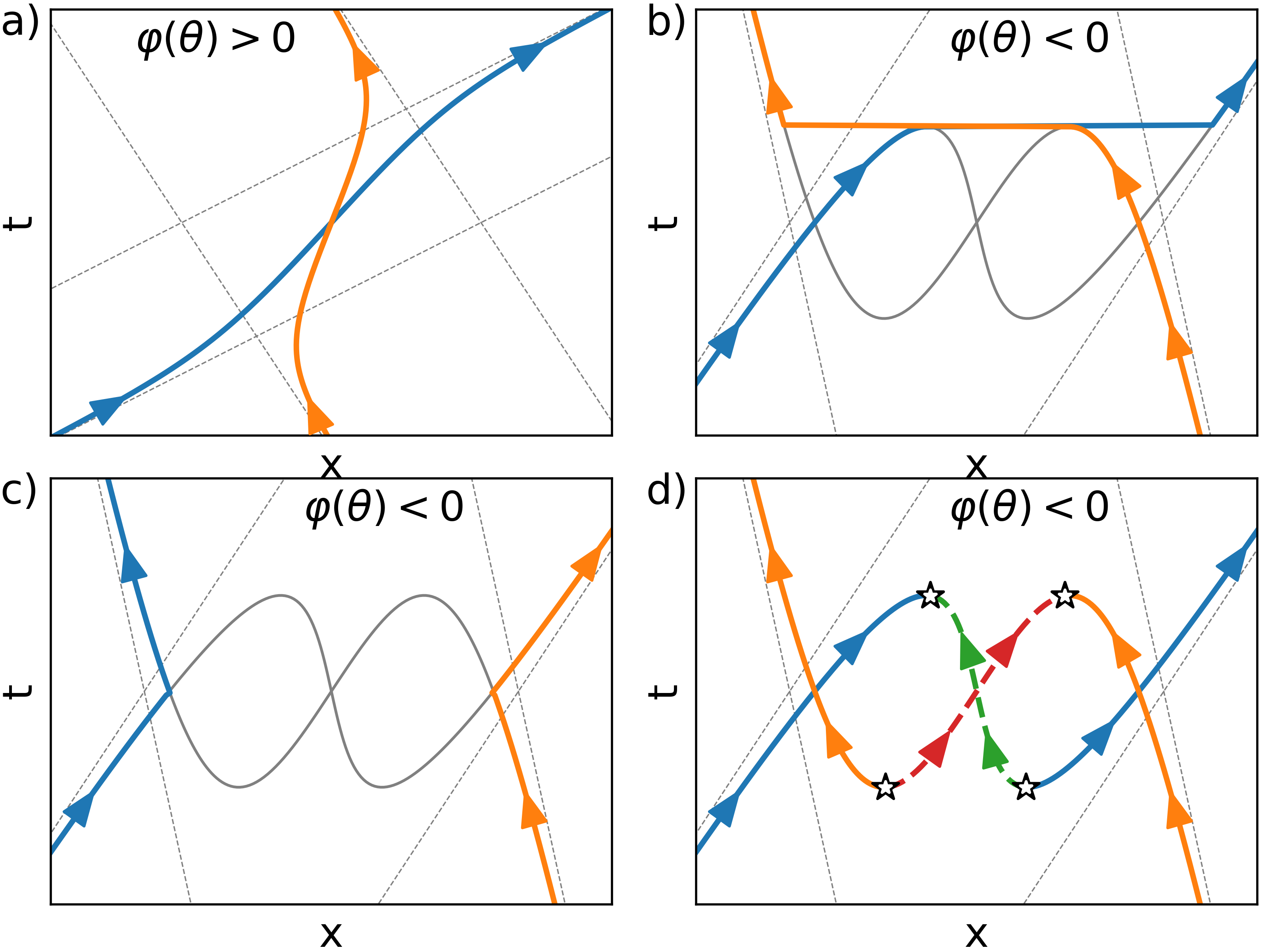
Figure 1: Trajectories of two particles during scattering for a) $\varphi(\theta)>0$ and b), c), d) $\varphi(\theta)<0$. The thin dashed lines are the asymptotic trajectories. We show three interpretations of the multivalued solutions for $\varphi(\theta)<0$: b) Particles jump instantaneous, c) particles are relabelled during collision, d) spontaneous creation of a particle-antiparticle pairs: The antiparticle annihilates with the incoming particle, leaving the new particle as outgoing particle.

Microscopic dynamics.— The effect of the interaction can be seen as a particle-dependent, dynamical change of metric from $x$- to $y$-space where it is free: the change of infinitesimal length is ${\rm d}y_{i}=K_{i}(x_{i}){\rm d}x_{i}$ where $K_{i}(x)=\big{(}1+\sum_{j\neq i}\partial_{\theta}\partial_{x}\psi(x-x_{j},\theta_{i}-\theta_{j})\big{)}$ measures the effective “free” space. It can best be pictured in the two-particle case, see Fig. 1 and SM . For $\varphi(\theta)>0$ (e.g. $\psi_{\rm ll}$) particles slow down during scattering, giving an effective backwards displacement (Fig. 1a) interpreted as the presence of additional, hidden space where particles must travel. If $\psi(x,\theta)=\frac{1}{2}\operatorname{sgn}(x)\phi(\theta)$ for some $\phi(\theta)$, they “stick” and acquire an internal clock that accounts for this extra space at collisions Doyon and Hübner (2023). For $\varphi(\theta)<0$, (2) does not necessarily have a unique solution. In case it does, particles speed up, giving an effective forward displacement and a reduction of effective space; hard rods of positive lengths are a limiting case, where the displacement – which traces the momentum being transferred – is instantaneous. However, if $\psi(x,\theta)$ varies on too small scales or scattering involves too many particles, solutions to (2) can become multivalued, and trajectories appear to go backward in time. The generating function (1) does not induce a canonical transformation on the standard phase space. One may consider three “regularisations”, without affecting the large-scale physics, all implementing a reduction of effective space. (i) Choose any branch; e.g. follow one branch until it disappears, then jump to another branch (Fig. 1b). This is similar to the flea gas Doyon et al. (2018b), but not Hamiltonian nor time reversible. (ii) Using the “hard-core” picture Cardy and Doyon (2022), relabel particles at the first collision (Fig. 1c). This gives a time-reversible dynamics (no longer a tracer dynamics), as long as such collisions always appear before any time-backward parts of trajectories; this re-labelling gives the rods in the hard-rod case. (iii) Inspired by Feynman’s picture, interpret time-backward parts of trajectories as antiparticles (Fig. 1d). The proximity of a particle (say orange in the figure) occasions a spontaneous particle-antiparticle pair creation (blue and green); the antiparticle (green) later annihilates with the incoming particle (blue) leaving the created particle (also blue) as outgoing physical particle. This is time-symmetric and can be used to define a Hamiltonian on the ‘Fock phase-space’ $\mathcal{F}=\bigoplus_{N}\mathbb{R}^{2N}$, where (1) should induce a canonical transformation. We now argue this picture naturally arises from $T\bar{T}$-deformations.

$T\bar{T}$-deformations.— Generalized $T\bar{T}$-deformations, as proposed in Doyon et al. (2022), are obtained as flows of Hamiltonians $H^{(\lambda)}\to H^{(\lambda)}+\delta H^{(\lambda)}$ parametrized by $\lambda$:

$$\delta H^{(\lambda)} =\delta\lambda\int{\rm d}\theta{\rm d}\alpha{\rm d}x{\rm d}x^{\prime}\,w(x-x^{\prime},\theta-\alpha)$$

$$\quad\times\big{(}q^{(\lambda)}_{\theta}(x)j^{(\lambda)}_{\alpha}(x^{\prime})-j^{(\lambda)}_{\theta}(x)q^{(\lambda)}_{\alpha}(x^{\prime})\big{)},$$ (5)

with $w(x,\theta)$ some deformation function. Here $q^{(\lambda)}_{\theta}(x)$ and $j^{(\lambda)}_{\theta}(x)$ are the charge densities and currents, with continuity equation $\partial_{t}q^{(\lambda)}_{\theta}+\partial_{x}j^{(\lambda)}_{\theta}=0$, associated to the charge $Q^{(\lambda)}_{\theta}=\sum_{i}\delta(\theta-\theta^{(\lambda)}_{i})$ that measures the density of asymptotic momenta at $\theta$ in the deformed system. It turns out that if $H$ is an integrable tracer dynamics, then so is $H^{(\lambda)}$, and $q^{(\lambda)}_{\theta}(x)$ and $j^{(\lambda)}_{\theta}(x)$ exist and are short-range. Remarkably, starting from a system of free particles $H^{(0)}=\sum_{i}p_{i}^{2}/2$, the deformed Hamiltonian $H^{(\lambda)}$ is nothing else but $H^{[\psi^{\lambda}]}$, Eq. (4), with $\psi^{\lambda}(x,\theta)=\lambda\int_{-\infty}^{\infty}{\rm d}x^{\prime}\,\operatorname{sgn}(x-x^{\prime})w(x^{\prime},\theta)$. This generalises the mass-momentum deformation yielding hard rods Cardy and Doyon (2022), see SM . The semiclassical Bethe systems are the first concrete example of generalized $T\bar{T}$-deformations. We have rigorous proofs of these statements Doyon et al. under conditions guaranteeing invertibility of (2), (3), where $H^{[\psi^{\lambda}]}$ can be constructed on the standard phase space.

Going further, here we make the crucial observation that the relation Eq. (2), be it invertible or not, is still the correct $T\bar{T}$-deformation of the impact-parameter-position relation $y_{i}=x_{i}$. Indeed, $T\bar{T}$-deformations (New classical integrable systems from generalized $T\bar{T}$-deformations) can be obtained as canonical flows Pozsgay et al. (2020); Kruthoff and Parrikar (2020); Cardy and Doyon (2022); Doyon et al. , and Eq. (2) arises directly from applying this flow. Thus, multivaluedness may appear along the $T\bar{T}$-flow, and pair creation/annihilation processes occur (Fig. 1d), as claimed; see SM . In all cases, the dynamics remains local.

Thermodynamics.— Let us consider the generalised Gibbs ensembles Ilievski et al. (2017), with Boltzmann weights $e^{-\sum_{a}\beta_{a}Q_{a}}$. We take more generally $(x,\theta)$-dependent Lagrange parameters varying on scale $L$, with $e^{-\int{\rm d}x{\rm d}\theta\,\beta(x/L,\theta)q_{\theta}(x)}=e^{-\sum_{i}\beta(x_{i}/L,\theta_{i})}$. In Doyon et al. we show, using methods of graph theory Kostov et al. (2018) and under certain further assumptions, that the free energy density

$$f_{L} =-\frac{1}{L}\log\sum_{N=0}^{\infty}\int\frac{{\rm d}^{N}x{\rm d}^{N}p}{N!}e^{-\sum_{i}\beta(x_{i}/L,\theta_{i}(\bm{x},\bm{p}))}$$ (6)

is finite and given by $f_{L}=-(2\pi L)^{-1}\int{\rm d}x{\rm d}\theta\,e^{-\varepsilon_{L}(x,\theta)}$ where the pseudo-energy $\varepsilon_{L}(x,\theta)$ satisfies

$$\varepsilon_{L}(x,\theta)=\beta(\tfrac{x}{L},\theta)-\int\frac{{\rm d}x^{\prime}{\rm d}\theta^{\prime}}{2\pi}\partial_{\theta}\partial_{x}\psi(x-x^{\prime},\theta-\theta^{\prime})e^{-\varepsilon_{L}(x^{\prime},\theta^{\prime})}.$$ (7)

This is a TBA-like equation for Maxwell-Boltzmann statistics (see e.g. Doyon (2020)). The TBA is well known from quantum Yang and Yang (1969); Takahashi (1999); Zamolodchikov (1990) and classical Bastianello et al. (2018); Spohn (2020); Doyon (2019); Koch et al. (2022); Koch and Bastianello (2023) integrability, at infinite volumes. It is striking that even at finite volumes the free energy possesses a TBA structure; the only result we are aware about this is for (positive-length) hard rods Percus (1976); Bulchandani (2023). We postulate that the finite-volume free energy in interacting quantum and classical integrable systems is given by Eq. (7) under an appropriate choice of $\partial_{\theta}\partial_{x}\psi(x,\theta)$ reproducing the scattering shift $\varphi(\theta)$. The infinite-volume limit of Eq. (7) yields the expected TBA equation $\varepsilon(\bar{x},\theta)=\lim_{L\to\infty}\varepsilon_{L}(L\bar{x},\theta)=\beta(\bar{x},\theta)-\int\frac{{\rm d}\theta^{\prime}}{2\pi}\varphi(\theta-\theta^{\prime})e^{-\varepsilon(\bar{x},\theta^{\prime})}$, from which $\lim_{L\to\infty}f_{L}$ follows. Thus the thermodynamics of the semiclassical Bethe systems is described by the standard machinery of TBA, including its “local density approximation”.

The free energy gives thermodynamic averages and fluctuations of conserved quantities. Interestingly, we also have the exact thermodynamic average $\rho_{\rm phys}(p)=n(\theta(p))/(2\pi)$ for the physical momentum distribution $L^{-1}\sum_{i}\delta(p-p_{i})$. Here $n(\theta)=e^{-\varepsilon(\theta)}$ is the occupation function and $\theta(p)$ is the inverse of the “Dressed momentum” function $p^{\rm Dr}(\theta)$. The latter is known to be the physical momentum of an excitation at Bethe root $\theta$ in Bethe ansatz systems, and is fixed by TBA equations. See SM . As physical momenta of particles change throughout their trajectories, $\rho_{\rm phys}(p)$ is a quantity that is typically hard to access in integrable models; this is the first exact expression that we are aware of.

GHD.— We provide a heuristic argument for GHD to emerge in the hydrodynamic limit, paralleling Ref. Doyon and Hübner (2023); other techniques Boldrighini et al. (1983) should give rigorous results.

We take macroscopic space and time, $x=L\bar{x},\,t=L\bar{t}$ ($\bar{x}$, $\bar{t}$ finite, $L\to\infty$), with scaled coordinates $\bar{x}_{i}(\bar{t})=x_{i}(t)/L$ and $\bar{y}_{i}=y_{i}/L$. The empirical density $\rho_{\rm e}(\theta,\bar{x},\bar{t})=L^{-1}\sum_{i}\delta(\bar{x}-\bar{x}_{i}(\bar{t}))\delta(\theta-\theta_{i})$, is assumed to converge “weakly”: $\rho_{\rm e}(\theta,\bar{x},\bar{t})\to\rho_{\rm p}(\theta,\bar{x},\bar{t})$. Clearly,

$$\partial_{\bar{t}}\rho_{\rm e}(\theta,\bar{x},\bar{t})+\partial_{\bar{x}}\Big{(}L^{-1}\sum_{i}\dot{\bar{x}}_{i}\delta(\bar{x}-\bar{x}_{i})\delta(\theta-\theta_{i})\Big{)}=0.$$ (8)

Re-writing Eq. (2) as $\bar{x}_{i}(\bar{t})=\bar{y}_{i}+\theta_{i}\bar{t}-\frac{1}{L}\sum_{j\neq i}\partial_{\theta}\psi(L(\bar{x}_{i}(\bar{t})-\bar{x}_{j}(\bar{t})),\theta_{i}-\theta_{j})$, we assume that, for every $i$, there is a fraction of particles $j$ that tend to 1 as $L\to\infty$ such that $\bar{x}_{i}(\bar{t})-\bar{x}_{j}(\bar{t})>0$. Then, we can replace $\partial_{\theta}\psi(L\bar{x},\theta)\to\psi^{\operatorname{sgn}(\bar{x})}\varphi(\theta)$ where $\psi^{+}-\psi^{-}=1$. Taking the $\bar{t}$-derivative, we find

$$\dot{\bar{x}}_{i}=\theta_{i}-\frac{1}{L}\sum_{j\neq i}\delta(\bar{x}_{i}-\bar{x}_{j})\varphi(\theta_{i}-\theta_{j})(\dot{\bar{x}}_{i}-\dot{\bar{x}}_{j})\qquad(L\to\infty).$$ (9)

Making the ansatz $\dot{\bar{x}}_{i}=f(\bar{x}_{i},\theta_{i})$, the second term on the right-hand side is $-\int{\rm d}\theta\,\rho_{\rm e}(\theta,\bar{x}_{i},\bar{t})\varphi(\theta_{i}-\theta)(f(\bar{x}_{i},\theta_{i})-f(\bar{x}_{i},\theta))$. Thus $f(\bar{x},\theta)=v^{\rm eff}_{[\rho_{\rm e}(\cdot,\bar{x},\bar{t}]}(\theta)$ solves

$$v^{\rm eff}_{[\rho]}(\theta)=\theta-\int{\rm d}\theta^{\prime}\,\rho(\theta^{\prime})\varphi(\theta-\theta^{\prime})(v^{\rm eff}_{[\rho]}(\theta)-v^{\rm eff}_{[\rho]}(\theta^{\prime})).$$ (10)

This is exactly the equation for the effective velocity in GHD Castro-Alvaredo et al. (2016); Bertini et al. (2016). Putting this into Eq. (8) and taking the limit $L\to\infty$ we obtain the GHD equation,

$$\partial_{\bar{t}}\rho_{\rm p}(\theta,\bar{x},\bar{t})+\partial_{\bar{x}}\big{(}v^{\rm eff}_{[\rho_{\rm p}]}(\theta,\bar{x},\bar{t})\rho_{\rm p}(\theta,\bar{x},\bar{t})\big{)}=0.$$ (11)

Thus, we have shown that, at large scales, the semiclassical Bethe system satisfies the GHD equation. This is not rigorous – in particular, in Eq. (9) one would need to use a regularization of the delta-function. We give an alternative derivation of GHD in SM , based on the fact that the metric change ${\rm d}y_{i}=K_{i}(x_{i}){\rm d}x_{i}$ converges to the GHD change of metric $K_{i}(x)\to 2\pi\rho_{\rm s}(\theta_{i},x)$ determined by the “space” or “total” density $\rho_{\rm s}(\theta,x)$ Doyon et al. (2018a).

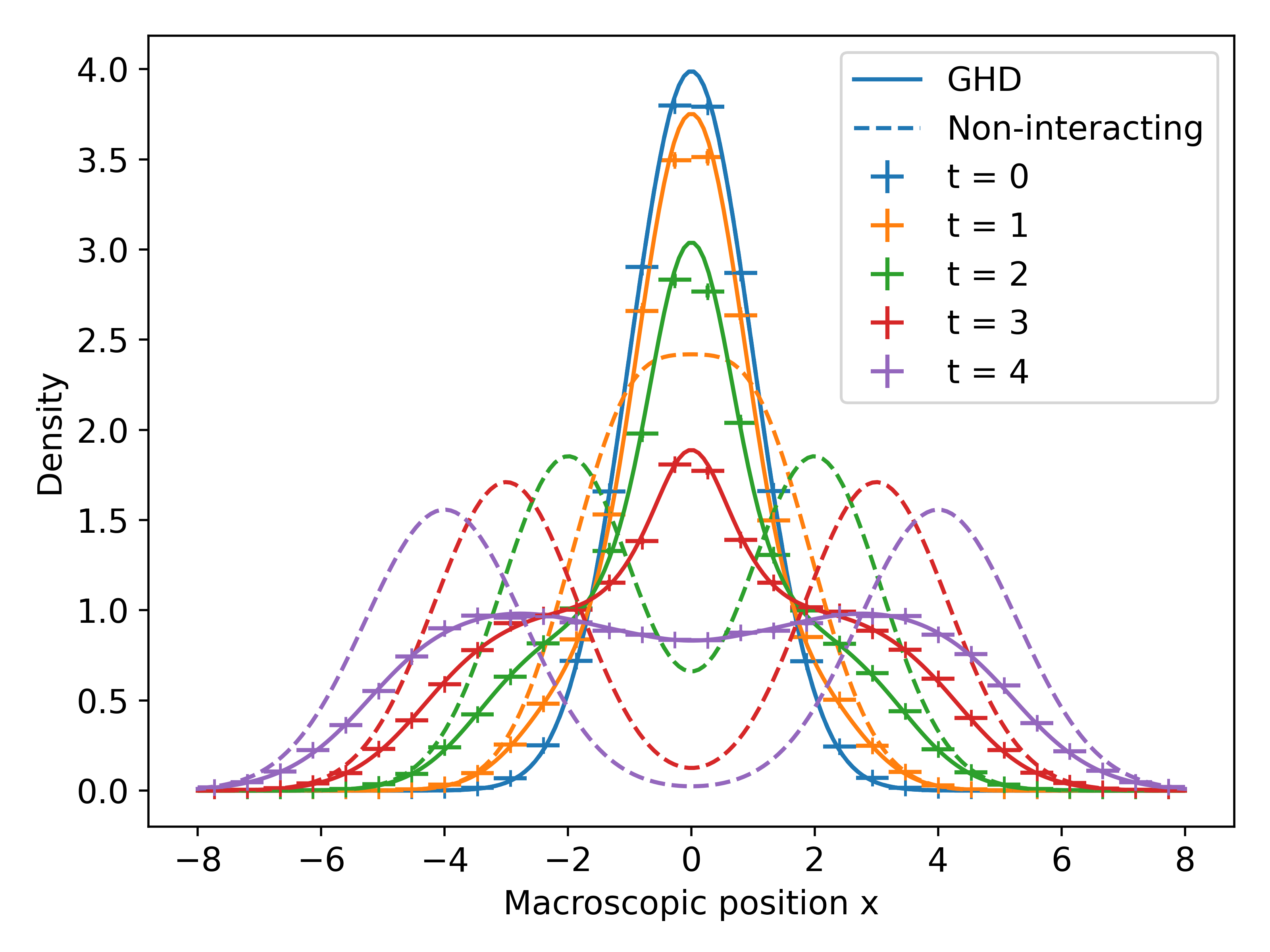
Figure 2: Evolution of the microscopic particle density (data points) and that from the GHD solution (solid lines) for different times. The initial state is $\rho_{\rm p}(\theta,x,0)=\frac{25}{2\pi}e^{-x^{2}/2}\left(e^{-25(\theta-1)^{2}/2}+e^{-25(\theta+1)^{2}/2}\right)$. We use $\psi(x,\theta)=\tfrac{x}{2\sqrt{x^{2}+\alpha^{2}}}\phi(\theta)$, where $\alpha=0.1$ and $\phi(\theta)=2\arctan{\tfrac{\theta}{c}}$. The microscopic results were averaged over $100$ samples, each starting from a randomly generated initial state ($L=300$, each sample contains $N\approx 3000$ particles). The error bars indicate the standard deviation and the bin size used for computing the density of particles. We also give the density for non-interacting particles (dashed lines) for comparision.

We numerically demonstrate that the GHD equation correctly captures the large-scale behaviour in an explicit example, see Fig. 2. For illustration, we use the phase shift from the quantum Lieb-Liniger model, but with an initial state that breaks the maximal fermionic occupation allowed by quantum mechanics (the maximal density of particle per state is $6.264>1$). This initial state is nevertheless realizable, and its hydrodynamics makes sense, as indeed it is realised by a semiclassical Bethe system. The details of the numerical simulations can be found in SM . Compared to the evolution of non-interacting particles the expansion of the interacting particles is much slower, which is in line with the intuitive meaning of a positive phase-shift as an effective time-delay during the scattering of two particles.

Conclusions.— We introduced a new class of classical integrable models, dubbed semiclassical Bethe systems for their relation with the quantum Bethe ansatz, obtained as generalized $T\bar{T}$-deformations of classical noninteracting particles. In these systems, each particle is a “tracer”: it has the same incoming and outgoing momentum. The class is parametrised by a function determining the microscopic dynamics, and displays factorised scattering with a (largely) arbitrary two-body shift, including those found in many quantum integrable models. The microscopic dynamics displays special features including pair creations / annihilations; the thermodynamics in finite volumes surprisingly takes a form akin to the thermodynamic Bethe ansatz (TBA), reducing to the TBA at infinite volume; the distribution in physical phase space can be evaluated exactly; and the large-scale dynamics is described by GHD, and therefore identical to that of any quantum/classical integrable system with the same chosen two-body shift. We conjecture that, with short-range interaction, the agreement persists at higher orders: the models should encode the universal hydrodynamic expansion of classical many-body integrability, as corrections due to specific interactions should be exponentially subleading. For instance, particles’ positions in our models should approximate well the spatial distribution of solitons in dense soliton gases, something that can be useful for initial state preparation.

It would be interesting to construct the full particle-non-conserving Hamiltonian description of trajectories (2), (3) with negative shifts $\varphi(\theta)<0$, Fig. 1d. Finding the full integrability structure of our models, perhaps connecting with sine-Gordon soliton trajectories Babelon and Bernard (1993); Babelon et al. (1996, 1997), would be interesting, as would quantising our models, perhaps in the spirit of Doyon and Hübner (2023) (integrability of generalized $T\bar{T}$-deformed systems is established Doyon et al. (2022)); the notion of pair creation / annihilation may play an important role. Finally, adding an external potential is possible, and we anticipate that rigorous proofs of the emergence of the GHD equation can be obtained following ideas in the hard-rod case Boldrighini et al. (1983); Ferrari et al. (2022). This might also shed light on GHD beyond the Euler scale.

Acknowledgements.— We are grateful to Olalla Castro Alvaredo for discussions, and to Joseph Durnin for previous collaboration on related subjects. FH acknowledges funding from the faculty of Natural, Mathematical & Engineering Sciences at King’s College London. BD was supported by the Engineering and Physical Sciences Research Council (EPSRC) under grant EP/W010194/1. The numerical simulations were done using the CREATE cluster CRE .

References

- Castro-Alvaredo et al. (2016) O. A. Castro-Alvaredo, B. Doyon, and T. Yoshimura, Phys. Rev. X 6, 041065 (2016).
- Bertini et al. (2016) B. Bertini, M. Collura, J. De Nardis, and M. Fagotti, Phys. Rev. Lett. 117, 207201 (2016).
- Schemmer et al. (2019) M. Schemmer, I. Bouchoule, B. Doyon, and J. Dubail, Phys. Rev. Lett. 122, 090601 (2019).
- Malvania et al. (2021) N. Malvania, Y. Zhang, Y. Le, J. Dubail, M. Rigol, and D. S. Weiss, Science 373, 1129 (2021), https://www.science.org/doi/pdf/10.1126/science.abf0147 .
- Wei et al. (2022) D. Wei, A. Rubio-Abadal, B. Ye, F. Machado, J. Kemp, K. Srakaew, S. Hollerith, J. Rui, S. Gopalakrishnan, N. Y. Yao, I. Bloch, and J. Zeiher, Science 376, 716 (2022), https://www.science.org/doi/pdf/10.1126/science.abk2397 .
- Spohn (1991) H. Spohn, Large Scale Dynamics of Interacting Particles (Springer Berlin Heidelberg, 1991).
- Doyon and Spohn (2017) B. Doyon and H. Spohn, J. Stat. Mech. Theory Exp. 2017, 073210 (2017).
- Ferrari et al. (2022) P. A. Ferrari, C. Franceschini, D. G. Grevino, and H. Spohn, preprint arXiv:2211.11117 (2022).
- Spohn (2020) H. Spohn, J. Stat. Phys. 180, 4 (2020).
- Doyon (2019) B. Doyon, J. Math. Phys. 60, 073302 (2019).
- Spohn (2022) H. Spohn, Journal of Mathematical Physics 63, 033305 (2022), https://pubs.aip.org/aip/jmp/article-pdf/doi/10.1063/5.0075670/16560227/033305_1_online.pdf .
- Koch et al. (2022) R. Koch, J.-S. Caux, and A. Bastianello, Journal of Physics A: Mathematical and Theoretical 55, 134001 (2022).
- Bulchandani et al. (2021) V. B. Bulchandani, M. Kulkarni, J. E. Moore, and X. Cao, Journal of Physics A: Mathematical and Theoretical 54, 474001 (2021).
- Bastianello et al. (2018) A. Bastianello, B. Doyon, G. Watts, and T. Yoshimura, SciPost Physics 4, 045 (2018).
- Koch and Bastianello (2023) R. Koch and A. Bastianello, SciPost Phys. 15, 140 (2023).
- Bastianello (2023) A. Bastianello, “The sine-gordon model from coupled condensates: a generalized hydrodynamics viewpoint,” (2023), arXiv:2310.04493 [cond-mat.stat-mech] .
- Bonnemain et al. (2022) T. Bonnemain, B. Doyon, and G. El, Journal of Physics A: Mathematical and Theoretical 55, 374004 (2022).
- El (2021) G. A. El, J. Stat. Mech. Theory Exp. 2021, 114001 (2021).
- Suret et al. (2023) P. Suret, S. Randoux, A. Gelash, D. Agafontsev, B. Doyon, and G. El, preprint arXiv:2304.06541 (2023).
- Boldrighini et al. (1983) C. Boldrighini, R. L. Dobrushin, and Y. M. Sukhov, J. Stat. Phys. 31, 577 (1983).
- Croydon and Sasada (2020) D. A. Croydon and M. Sasada, Commun. Math. Phys. 383, 427 (2020).
- El (2003) G. El, Physics Letters A 311, 374 (2003).
- El and Kamchatnov (2005) G. A. El and A. M. Kamchatnov, Phys. Rev. Lett. 95, 204101 (2005).
- El and Tovbis (2020) G. El and A. Tovbis, Physical Review E 101, 052207 (2020).
- Bertini et al. (2022) B. Bertini, F. H. L. Essler, and E. Granet, Phys. Rev. Lett. 128, 190401 (2022).
- Doyon and Hübner (2023) B. Doyon and F. Hübner, preprint arXiv:2307.09307 (2023), arXiv:arXiv:2307.09307 [cond-mat.stat-mech] .
- Cubero et al. (2021) A. C. Cubero, T. Yoshimura, and H. Spohn, J. Stat. Mech. Theory Exp. 2021, 114002 (2021).
- Borsi et al. (2021) M. Borsi, B. Pozsgay, and L. Pristyák, J. Stat. Mech. Theory Exp. 2021, 094001 (2021).
- Zamolodchikov (2004) A. B. Zamolodchikov, preprint arXiv:hep-th/0401146 (2004), arXiv:arXiv:hep-th/0401146 .
- Cavaglià et al. (2016) A. Cavaglià, S. Negro, I. M. Szécsényi, and R. Tateo, JHEP 2016, 112 (2016).
- Smirnov and Zamolodchikov (2017) F. A. Smirnov and A. B. Zamolodchikov, Nucl. Phys. B 915, 363 (2017), arXiv:1608.05499 .
- Castro-Alvaredo et al. (2023a) O. A. Castro-Alvaredo, S. Negro, and F. Sailis, JHEP 09, 048 (2023a), arXiv:2306.01640 [hep-th] .
- Castro-Alvaredo et al. (2023b) O. A. Castro-Alvaredo, S. Negro, and F. Sailis, preprint arXiv:2305.17068 (2023b), arXiv:2305.17068 [hep-th] .
- Castro-Alvaredo et al. (2023c) O. A. Castro-Alvaredo, S. Negro, and I. M. Szécsényi, preprint arXiv:2311.16955 (2023c), arXiv:2311.16955 [cond-mat.stat-mech] .
- Pozsgay et al. (2020) B. Pozsgay, Y. Jiang, and G. Takács, JHEP 2020, 92 (2020).
- Pozsgay et al. (2021a) B. Pozsgay, T. Gombor, A. Hutsalyuk, Y. Jiang, L. Pristyák, and E. Vernier, Phys. Rev. E 104, 044106 (2021a).
- Pozsgay et al. (2021b) B. Pozsgay, T. Gombor, and A. Hutsalyuk, Phys. Rev. E 104, 064124 (2021b).
- Esper and Frolov (2021) C. Esper and S. Frolov, JHEP 2021, 1 (2021).
- Cardy and Doyon (2022) J. Cardy and B. Doyon, JHEP 2022, 1 (2022).
- Jiang (2022) Y. Jiang, SciPost Physics 12, 191 (2022).
- Borsi et al. (2023) M. Borsi, L. Pristyák, and B. Pozsgay, Phys. Rev. Lett. 131, 037101 (2023).
- Jiang (2021) Y. Jiang, Commun. Theor. Phys. 73, 057201 (2021).
- Doyon et al. (2022) B. Doyon, J. Durnin, and T. Yoshimura, SciPost Phys. 13, 072 (2022).
- Ilievski et al. (2016) E. Ilievski, M. Medenjak, T. Prosen, and L. Zadnik, J. Stat. Mech. Theory Exp. 2016, 064008 (2016).
- De Nardis et al. (2022) J. De Nardis, B. Doyon, M. Medenjak, and M. Panfil, J. Stat. Mech. Theory Exp. 2022, 014002 (2022).
- Conti et al. (2019) R. Conti, S. Negro, and R. Tateo, JHEP 2019 (2019), 10.1007/jhep02(2019)085.
- Doyon et al. (2018a) B. Doyon, H. Spohn, and T. Yoshimura, Nucl. Phys. B 926, 570 (2018a).
- Doyon (2020) B. Doyon, SciPost Phys. Lect. Notes , 18 (2020).
- Note (1) We became aware of this after we obtained our results.
- Bulchandani (2023) V. B. Bulchandani, preprint arXiv:2309.15846 (2023).
- (51) B. Doyon, F. Hübner, and T. Yoshimura, to appear .
- Zamolodchikov and Zamolodchikov (1979) A. B. Zamolodchikov and A. B. Zamolodchikov, Ann. Phys. 120, 253 (1979).
- (53) See the Supplemental Material for an analysis of the equations for two particles, a description of the numerical simulations, an alternative argument for deriving the GHD equations, and a derivation of the physical phase-space density.
- Doyon et al. (2018b) B. Doyon, T. Yoshimura, and J.-S. Caux, Phys. Rev. Lett. 120, 045301 (2018b).
- Kruthoff and Parrikar (2020) J. Kruthoff and O. Parrikar, SciPost Phys. 9, 78 (2020).
- Ilievski et al. (2017) E. Ilievski, E. Quinn, and J.-S. Caux, Phys. Rev. B 95, 115128 (2017).
- Kostov et al. (2018) I. Kostov, D. Serban, and D.-L. Vu, in Quantum Theory and Symmetries with Lie Theory and Its Applications in Physics Volume 2, edited by V. Dobrev (Springer Singapore, Singapore, 2018) pp. 77–98.
- Yang and Yang (1969) C. N. Yang and C. P. Yang, J. Stat. Phys. 10, 1115 (1969).
- Takahashi (1999) M. Takahashi, Thermodynamics of One-Dimensional Solvable Models (Cambridge University Press, 1999).
- Zamolodchikov (1990) A. Zamolodchikov, Nucl. Phys. B 342, 695 (1990).
- Percus (1976) J. K. Percus, J. Stat. Phys. 15, 505 (1976).
- Babelon and Bernard (1993) O. Babelon and D. Bernard, Phys. Lett. B 317, 363 (1993).
- Babelon et al. (1996) O. Babelon, D. Bernard, and F. Smirnov, Commun. Math. Phys. 182, 319 (1996).
- Babelon et al. (1997) O. Babelon, D. Bernard, and F. Smirnov, Nucl. Phys. B-Proceedings Supplements 58, 21 (1997).
- (65) “King’s College London. (2022). King’s Computational Research, Engineering and Technology Environment (CREATE). Retrieved June 30, 2023, from https://doi.org/10.18742/rnvf-m076,” .