Reply to “Comment on “Advanced Testing of Low, Medium, and High ECS CMIP6 GCM Simulations Versus ERA5-T2m” by N. Scafetta (2022)” by Schmidt, Jones, and Kennedy (2023)

Abstract

Schmidt, Jones & Kennedy (SJK) (2023, https://doi.org/10.1029/2022GL102530, submited to GRL)’s critique of Scafetta (2022, https://doi.org/10.1029/2022GL097716) is flawed. Their assessment of the error of the ERA-T2m 2011–2021 mean ($\approx 0.10\;{{}^{\circ}}\mathrm{C}$) is 5-10 times overestimated and contradicts published literature. SJK confused natural variability with random noise, and mistook the error of the mean of a temperature chronology for the stochastic error of the regression parameter $M$ of a nonphysical isothermal climate model ($T(t)=M$). SJK’s allegations regarding the internal variability of the models, the role of the global climate model ensemble members, and other issues were partially addressed in Scafetta (2022, https://doi.org/10.1029/2022GL097716) and, later, more extensively in Scafetta (2023a, https://doi.org/10.1007/s00382-022-06493-w) where Scafetta (2022, https://doi.org/10.1029/2022GL097716)’s conclusions were confirmed.

¹Department of Earth Sciences, Environment and Georesources, University of Naples Federico II, Complesso Universitario di Monte S. Angelo, via Cinthia, 21, 80126 Naples, Italy.

Graphical Abstract

Cite as: Scafetta N. (2023). Reply to “Comment on “Advanced Testing of Low, Medium, and High ECS CMIP6 GCM Simulations Versus ERA5-T2m” by N. Scafetta (2022)” by Schmidt, Jones, and Kennedy (2023). Geophysical Research Letters 50, e2023GL104960. https://doi.org/10.1029/2023GL104960

Plain language summary

Schmidt, Jones & Kennedy (SJK) (2023, https://doi.org/10.1029/2022GL102530, submitted to GRL)’s assessment of the error of the ERA-T2m 2011–2021 mean ($\sigma_{\mu,95\%}=0.10\;{{}^{\circ}}\mathrm{C}$) incorrectly assumes that, during such a period, the global surface temperature was constant ($T(t)=M$) and that its interannual variability ($\Delta T_{i}=T_{i}-T(t_{i})=T_{i}-M$) was random noise. This is a nonphysical interpretation of the climate system that inflates the real error of the temperature mean by 5-10 times. In fact, the analysis of the ensemble of the global surface temperature members yields a decadal-scale error of about 0.01-0.02$\;{{}^{\circ}}\mathrm{C}$, as reported in published records and deduced from the Gaussian error propagation formula (GEPF) of a function of several variables (such as the mean of a temperature sequence of 11 different years) (Taylor, 1997, chapters 3 and 9). Instead, SJK assessed such error using the standard deviation of the mean (SDOM) (Taylor, 1997, chapter 4), which is an equation that can only be used when there exists a distribution of repeated measurements of the same variable (which is not the present case). Furthermore, SJK misinterpreted Scafetta (2022, https://doi.org/10.1029/2022GL097716) and ignored published literature such as Scafetta (2023a, https://doi.org/10.1007/s00382-022-06493-w) that already contradicted their main claim about the role of the internal variability of the models and confirmed the results of Scafetta (2022, https://doi.org/10.1029/2022GL097716).

Keywords: Global climate models; Global surface temperature; Chaotic systems; Stochastic processes

Keypoints

• Schmidt et al. (2023, https://doi.org/10.1029/2022GL102530, submitted to GRL) assessed the error of the temperature mean by erroneously using the SDOM instead of the error propagation formula.

• The interannual temperature variability is physical signal, not noise; the 2011–2021 ERA5-T2m mean error is not 0.10 °C, but 0.01-0.02 °C.

• The role of the internal variability of the models was extensively addressed in Scafetta (2023a, https://doi.org/10.1007/s00382-022-06493-w), who confirmed Scafetta (2022, https://doi.org/10.1029/2022GL097716).

Blog Comment

Scafetta, N.: Comment and Reply to GRL on evaluation of CMIP6 simulations, Climate Etc., (2023)
https://judithcurry.com/2023/09/24/comment-and-reply-to-grl-on-evaluation-of-cmip6-simulations/

1 Introduction

According to Schmidt, Jones & Kennedy (2023) (SJK2023), Scafetta (2022) (S2022) contains “numerous conceptual and statistical errors that undermine all of the conclusions”. SJK2023 reiterates the erroneous claims published in Real Climate on March 30, 2022 (Schmidt et al., 2022) and on October 10, 2022 (Schmidt, 2022).

Meanwhile, S2022 is now supported by the publication of other three works: Scafetta (2023a, b) provided a more comprehensive analysis of the same topic; Lewis (2023) reassessed downward the likely range of the equilibrium climate sensitivity (ECS) previously estimated by Sherwood et al. (2020). These three studies support S2022’s conclusion that $\mathrm{ECS}\leq 3.0\;{{}^{\circ}}\mathrm{C}$.

Herein, I demonstrate that SJK2023 is flawed. Section 2 overviews S2022 and follow-up works and highlights some of SJK2023’s key misinterpretations of S2022. SJK2023’s key criticism regarding the error of the mean—the only part of their argument supported by a calculation—is thoroughly rebutted in Section 3. Section 4 briefly addresses the internal variability issue using the same results reported in S2022’s Table 1; the extended analysis is found in Scafetta (2023a). Section 5 briefly discusses the other critiques.

2 Overview of Scafetta (2022) and Subsequent Works

S2022 measured the global surface warming from Jan/1980–Dec/1990 to Jan/2011–Jun/2021 based on the ERA5–T2m record (Hersbach et al., 2020) and compared it with the ensemble average hindcasts produced by 38 CMIP6 global climate models (GCMs) downloaded from KNMI Climate Explorer (https://climexp.knmi.nl/start.cgi). The historical forcing functions (1850–2014) and three distinct shared socioeconomic pathway scenarios (SSP2-4.5, SSP3-7.0, and SSP5-8.5; 2015–2100) were used for a total of 107 simulations (Scafetta, 2022, Table 1). S2022 aggregated the CMIP6 GCMs into three sub-ensembles, herein labeled “macro-GCMs”, according to their ECS value: Low-ECS ($1.5<\mathrm{ECS}\leq 3.0\;{{}^{\circ}}\mathrm{C}$); Medium-ECS ($3.0<\mathrm{ECS}\leq 4.5\;{{}^{\circ}}\mathrm{C}$), and High-ECS ($4.5<\mathrm{ECS}\leq 6.0\;{{}^{\circ}}\mathrm{C}$). The Low-ECS macro-GCM well hindcasted the observed warming; the Medium- and High-ECS macro-GCMs consistently showed a warm bias, suggesting that these two macro-GCMs may not be reliable climate predictors for climate-change policies.

SJK2023 did not acknowledge that S2022’s goal was to test three macro-GCMs, nor that S2022 examined three average simulations for each model (when available), which partially accounted for the uncertainty related to the GCMs’ internal variability, nor that Scafetta (2023a) extensively analyzed all CMIP6 GCM simulations available on KNMI Climate Explorer, which included 143 GCM ensemble average records and 688 GCM member simulations. Finally, Scafetta (2023b) examined the 175 CMIP6 GCM simulations that Schmidt proposed as indicative of the CMIP6 GCMs (Hausfather et al., 2022, Supplementary file). Scafetta (2023a, b) confirmed the warm bias of the Medium- and High-ECS macro-GCMs.

3 The error of the mean

According to SJK2023, S2022 overlooked the ERA5-T2m error of the mean from 2011 to 2021. SJK claimed that, in order to calculate the error of the mean (95% confidence), one must calculate the standard deviation of the annual temperature anomalies around their 11-year mean and multiply it by $1.96/\sqrt{N}$ (where $N=11$ is the number of years from 2011 to 2021),

$$\sigma_{95\%}=1.96\times\frac{\sigma_{inter\,annual}}{\sqrt{N}}=1.96\times\frac{1}{\sqrt{N}}\sqrt{\frac{\sum_{i=1}^{N}(T_{i}-\mu)^{2}}{N-1}}=0.10\;{{}^{\circ}}C,$$ (1)

where $T_{i}$ are the $N=11$ annual temperature values from 2011 to 2021 and

$$\mu=\frac{1}{N}\sum_{i=1}^{N}T_{i}$$ (2)

is their mean over the 11-year period: see Figure 1A.

However, as Scafetta (2023a, Appendix) already explained, Eq. 1 is wrong because the global surface temperature uncertainty from 2011 to 2021 at the decadal mean is typically estimated to be about $0.02\>{{}^{\circ}}\mathrm{C}$: see Figure 1C. In fact, Eq. 2 is a function of $N$ separate quantities rather than the mean of a distribution of $N$ repeated measurements of the same quantity. Thus, as explained below, its error cannot be calculated with the standard deviation of the mean (SDOM) of a (here-nonexistent) distribution of one quantity (Taylor, 1997, chapter 4), but must be computed with the Gaussian error propagation formula (GEPF) of a function of several quantities (Taylor, 1997, chapters 3 and 9).

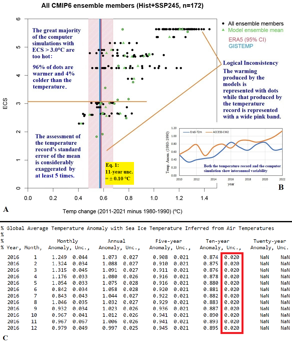
Figure 1: (A) SJK2023’s figure displaying the actual and simulated temperature changes from 1980–1990 to 2011–2021. The green dots represent a small subset of the model ensemble averages examined in S2022. (B) The insert shows that both the actual temperature record and computer simulations present inter-annual variability. My critiques (highlighted in the blue comments) are better detailed in the text. (C) Screenshot of the Berkeley Earth’s global surface temperature record (https://berkeley-earth-temperature.s3.us-west-1.amazonaws.com/Global/Land_and_Ocean_complete.txt) with its estimated (95% confidence) errors (Rohde et al., 2020). The red box highlights the typical error of the 10-year mean centered in 2016 ($\pm$0.020°C), which contradicts SJK2023’s Eq. 1 ($\pm$0.10°C).

3.1 Distinction Between the “Mean” and the  Regression Isothermal Model “$T(t)=M$”

GEPF establishes that the error of a generic function $q(z_{1},...,z_{N})$ of N different physical variables $z_{1},...,z_{N}$, each of which is estimated with $K$ stochastic measurements $z_{i,k=1,...,K}$, is

$$\sigma_{q}=\mathit{\sqrt{\sum_{i=1}^{N}\sum_{j=1}^{N}\frac{\partial q}{\partial z_{i}}\frac{\partial q}{\partial z_{j}}\cdot\sigma_{z_{i},z_{j}}}}=\mathit{\sqrt{\sum_{i=1}^{N}\left(\frac{\partial q}{\partial z_{i}}\right)^{2}\sigma_{z_{i}}^{2}+2\sum_{i=1}^{N-1}\sum_{j=i+1}^{N}\frac{\partial q}{\partial z_{i}}\frac{\partial q}{\partial z_{j}}\cdot\sigma_{z_{i},z_{j}}}}$$ (3)

where

$$\sigma_{z_{i},z_{j}}=\mathrm{cov}(z_{i},z_{j})=\frac{1}{K-1}\sum_{k=1}^{K}(z_{i,k}-\bar{z}_{i})(z_{j,k}-\bar{z}_{j})$$ (4)

is the covariance between $z_{i}$ and $z_{j}$: see https://en.wikipedia.org/wiki/Propagation_of_uncertainty; JCGM (2008, Eq. 13); Taylor (1997, Eq. 9.9). Note that $\sigma_{z_{i},z_{i}}=\sigma_{z_{i}}^{2}$ is the variance of each variable $z_{i}$, and the partial derivatives are calculated at the average values $\bar{z}_{i}$. Eq. 3 derives from a first-order Taylor series expansion of the function $q(z_{1},...,z_{N})$ applied to stochastic variables.

3.1.1 Definition of the Error of the Mean: “$\sigma_{\mu,95\%}$”

If $q(z_{1},...,z_{N})=\sum_{i=1}^{N}z_{i}/N=\mu$, we have $\partial q/\partial z_{i}=1/N$ and Eq. 3 becomes

$$\sigma_{\mu}=\frac{1}{N}\mathit{\sqrt{\sum_{i=1}^{N}\sigma_{z_{i}}^{2}+2\sum_{i=1}^{N-1}\sum_{j=i+1}^{N}\sigma_{z_{i},z_{j}}}}$$ (5)

If the $N$ physical quantities $z_{i}$ are also characterized by random and independent uncertainties, which means $\sigma_{z_{i},z_{j}}=0$ if $i\neq j$, Eq. 5 becomes

$$\sigma_{\mu}=\frac{1}{N}\mathit{\sqrt{\sum_{i=1}^{N}\sigma_{z_{i}}^{2}}}$$ (6)

(Taylor, 1997, Eqs. 3.16 and 3.47).

Therefore, if $T_{i}\pm\sigma_{i}$, for $i=1,2,...,N$, denote the global surface temperatures of 11 different years and their errors $\sigma_{i}$ are independent, their mean and its error are

$$\mu\pm\sigma_{\mu}=\frac{1}{N}\sum_{i=1}^{N}\left(T_{i}\pm\sigma_{i}\right)\approx\frac{1}{N}\sum_{i=1}^{N}T_{i}\pm\frac{1}{N}\sqrt{\sum_{i=1}^{N}\sigma_{i}^{2}}.$$ (7)

Thus,

$$\sigma_{\mu,95\%}=1.96\times\frac{\sqrt{\sum_{i=1}^{N}\sigma_{i}^{2}}}{N}=1.96\times\frac{1}{\sqrt{N}}\sqrt{\frac{\sum_{i=1}^{N}\sigma_{i}^{2}}{N}}=1.96\times\frac{\overline{\sigma}}{\sqrt{N}},$$ (8)

where

$$\overline{\sigma}^{2}=\frac{1}{N}\sum_{i=1}^{N}\sigma_{i}^{2}.$$ (9)

Eq. 8 differs from Eq. 1 because $\overline{\sigma}^{2}$ is not defined as the variance of the data-set around its mean, but as the mean of the variances of the data-points (Eq. 9).

Eq. 5 should be used when the temperature record is represented by an ensemble of K alternative records. The statistics resulting from different temperature records is addressed in Scafetta (2023a). In general, if the record permits to evaluate the data-point error covariance, $\sigma_{\mu}$ must be calculated with Eq. 5, which establishes that

$$0\leq\sigma_{\mu}\leq\frac{1}{N}\sum_{i=1}^{N}\sigma_{i},$$ (10)

(Taylor, 1997, Eqs. 3.17 and 3.48).

For example, the mean between 10 and 20 is 15. If the numbers are affected by independent Gaussian uncertainties, let’s say $x=10\pm 1$ and $y=20\pm 1$, their mean is $15\pm 0.7$ (Eq. 7). If their errors covary, the mean is $15\pm 0$ if $\sigma_{x,y}=-1$ or $15\pm 1$ if $\sigma_{x,y}=+1$ (Eq. 5). However, Eq. 1 calculates $15\pm 5$ even when 10 and 20 indicate two different quantities and are error-free, which is wrong.

3.1.2 Definition of the error of the isothermal regression parameter $M$: “$\sigma_{M,95\%}$”

In fact, Eq. 1 indicates something conceptually very different from the error of the mean of $N$ different temperature quantities. Eq. 1 indicates the standard deviation $\sigma_{M}$ of the coefficient “$M$” of the regression model

$$T(t)=M,$$ (11)

which postulates a strict physical temporal evolution of the global surface temperature from 2011 to 2022.

The regression coefficient $M$ is numerically equal to $\mu$, but their standard errors differ from each other because of the specific physical meaning that Eq. 11 has. In fact, Eq. 11 represents an isothermal climatic system. A model of this kind postulates that from 2011 to 2021, the “true” global surface temperature was constant and equal to $M$ for each year and, consequently, that the temperature anomalies from $M$,

$$\Delta T_{i}=T_{i}-T(t_{i})=T_{i}-M,\qquad\qquad\mathrm{for}\qquad i=1,...,N,$$ (12)

were $N$ independent random numbers belonging to a zero-mean Gaussian distribution with standard deviation equal to

$$\sigma_{\Delta T}=\sqrt{\frac{\sum_{i=1}^{N}(T_{i}-M)^{2}}{N-1}}.$$ (13)

Under such hypothesis, the error of $M$ is

$$\sigma_{M,95\%}=1.96\times\sigma_{M}=1.96\times\frac{\sigma_{\Delta T}}{\sqrt{N}}=1.96\times\frac{1}{\sqrt{N}}\sqrt{\frac{\sum_{i=1}^{N}(T_{i}-M)^{2}}{N-1}},$$ (14)

which is Eq. 1. If each data-point is also affected by a measurement error $\sigma_{i}$, Eq. 14 is rewritten as

$$\sigma_{M,95\%}=1.96\times\sqrt{\frac{\sigma_{\Delta T}^{2}+\bar{\sigma}^{2}}{N}}>1.96\times\frac{\overline{\sigma}}{\sqrt{N}}=\sigma_{\mu,95\%},$$ (15)

where $\overline{\sigma}^{2}=\frac{1}{N}\sum_{i=1}^{N}\sigma_{i}^{2}$.

Eq. 15 shows that the error of the regression parameter $M$ is different, and can also be significantly larger than the error of the mean $\mu$ as deduced from the data uncertainties (Eq. 8). Thus, postulating Eq. 11 and that the anomalies $\Delta T_{i}$ are random noise artificially increases the variance of the temperature data-points from $\sigma_{i}^{2}$ to $\sigma_{i}^{2}+\sigma_{\Delta T}^{2}$ and, therefore, also increases the uncertainty of their mean.

Eq. 13 can also be interpreted as a particular case of Eq. 3 when $N=1$, $q(z)=z$ and $\partial q/\partial z=1$; that is, when there only are $K$ repeated measurements of the “same” physical quantity $z$. Then, Eq. 14 (or Eq. 1) is the SDOM of the distribution of the $K$ measurements of $z$ (Taylor, 1997, Eqs. 4.9 and 4.14).

3.2 Discussion

The error of the 2011–2021 temperature mean is an observable that solely depends on the given errors of the temperature data: if the data are error-free, so is their mean. This error is unrelated to the standard deviation of the constant coefficient of any hypothetical regression model of the data (e.g. Eq. 11), whose error varies as the model changes.

SJK2023 assumed that the temperature anomalies $\Delta T_{i}$ (Eq. 12) were some kind of random noise produced by a mysterious stochastic process that they labeled “random nature”. The annual standard error of this unidentified stochastic process was claimed to be $\sigma_{year,95\%}=0.1\sqrt{11}=0.33\;{{}^{\circ}}\mathrm{C}$, which is one order of magnitude greater than the known annual stochastic error of these data (cf. Table 1). Such an assumption physically implies that from 2011 to 2021 the actual climate was isothermal, $T(t)=M$, which is nonphysical. The same assumption statistically implies that the 11 annual global surface temperatures from 2011 to 2021 are 11 repeated stochastic measurements of their 11-year mean, which is incorrect.

Eq. 1 can only be used when dealing with repeated measurements of the “same” physical quantity (Taylor, 1997, chapter 4). This occurs, for example, when several thermometers simultaneously measure the temperature of the same location. In such instances, the measurement discrepancies among the thermometers can be physically interpreted as generated by stochastic processes. Yet, 11 numbers, each indicating the annual global surface temperature of a different year, are not 11 repeated measurements of their 11-year mean; different years reflect separate physical states of the climate, each with its own temperature, and a 1-year period is not an 11-year period. Thus, the 11 temperatures do not represent a stochastic distribution of one quantity but 11 different quantities. Therefore, the error of their mean cannot be calculated with the SDOM (Eq. 1), but only with the GEPF (Eq. 6, or, in general, Eq. 5).

The interannual temperature variability is not “noise” or some kind of “error” because it is due to well-known physical mechanisms such as ENSO fluctuations, volcanic eruptions, variations in solar activity, anthropogenic and natural warming trends, etc. Eq. 11 can only be replaced with a realistic physical model of the type

$$T(t)=M+\Delta T_{physical}(t),$$ (16)

where $M$ is the mean and the function $\Delta T_{physical}(t)$ captures the actual interannual physical component of the record, which should coincide with the experimental measurements within their errors of measure. $\Delta T_{physical}(t)$ can derive from external forcings and/or internal mechanisms. Scafetta (2023a, Appendix) showed that when this exercise is done, the error of $M$ approaches the error of the mean (Eq. 8). In fact, all temperature records resemble the same temperature fluctuations, indicating that those changes are primarily physical signal and not noise. As a result, if no other kind of random error can be physically demonstrated, the natural interannual variability of ERA5-T2m cannot increase the statistical error of its 2011–2021 temperature mean.

Scafetta (2023a) outlined other serious contradictions with applying Eq. 1. For example, by replacing the annual ($N=11$) with the monthly ($N=132$) temperature record, the value of $\sigma_{\mu,95\%}$ calculated by Eq. 1 changes from about $0.108$ to $0.034\;{{}^{\circ}}\mathrm{C}$. However, for records made of genuine stochastic Gaussian fluctuations, $\sigma_{\mu,95\%}$ is independent of the time-scale of the data. Thus, statistics excludes that ERA5-T2m consists of random Gaussian fluctuations around a decadal mean. Therefore, SJK2023’s calculation is arbitrary because Eq. 1 highly depends on the temporal resolution of the data. This inconsistency persists even if SJK2023’s isothermal model (Eq. 11) were replaced with a linear model (a referee proposal) because by simply interpolating the data with additional points, the error of its constant coefficient converges to zero  as N increases (Taylor, 1997, Eq. 8.16) because the data variance around the model prediction will not change much since the data-points are physically inter-correlated.

Figure 1A shows another severe logical, physical, and mathematical inconsistency: SJK2023 estimated $\sigma_{M,95\%}$ (Eq. 1 or 14) just for the ERA-T2m temperature record and showed it with a $\pm 0.10\;{{}^{\circ}}\mathrm{C}$ pink-bar. However, for the 208 (36 green + 172 black dots) GCM hindcasts, they calculated $\sigma_{\mu,95\%}$ (Eq. 8). The latter are correctly represented by dots since the simulations are unaffected by any statistical error while showing significant interannual variability like ERA-T2m, as Figure 1B demonstrates. Yet, the same algorithm must be used for both the real and synthetic temperature records.

It must also be mentioned that evaluating the 2011–2021 temperature mean and its error does not depend on the GCMs’ performance in modeling the observed inter-annual climatic variability, nor on the possibility of predicting the “timing of El-Niño events”. Moreover, these events do not possess any “random nature”, as SJK2023 claimed by confusing a weakly chaotic system, like the climate, with a stochastic process. Only the quantum world presents instances of true randomness. In fact, while forecasting the “timing of El-Niño events” may be challenging (chaotic system), an El-Niño event is a well-established fact when historically recorded. Yet, Eq. 1 erroneously implies that the annual temperature data are prone to stochastic errors that are so excessively large ($\sigma_{year,95\%}=0.33\;{{}^{\circ}}\mathrm{C}$) that it may not even be possible to determine (stochastic process) whether or not an El-Niño event has occurred in any given year.

In other words, since we are interested in determining what happened from 2011 to 2021, the 2011–2021 ERA5-T2m interannual variability—which represents the actual climatic chronology that occurred—cannot be replaced by random data and, accordingly, Eq. 1 cannot be applied to it. SJK somehow misunderstood that only the internal variability of the GCMs can generate stochastic ensembles of interannual hindcasts by randomly varying their initial conditions or internal parameters. However, ERA5-T2m is not a GCM, but the given temperature chronology that produces only one 2011–2021 temperature mean with its own error of measure.

3.3 Estimation of the likely “error of the mean” for the ERA-T2m 2011-2021 record

S2022 did not report the error of the mean because the ERA-T2m monthly or annual uncertainties had not been explicitly published (Hersbach et al., 2020). However, such error was expected to be negligible because, as Scafetta (2023a) explained, over the last 50 years, the annual temperature uncertainties are estimated to be 0.03-$0.05\;{{}^{\circ}}\mathrm{C}$ (95% confidence) by all global surface temperature records (Lessen et al., 2019; Morice et al., 2021; Rohde et al., 2020) and, if their error-covariance is ignored, such uncertainties should be divided by $\sqrt{11}$ to get the error at the 11-year scale (Eq. 8).

For example, Table 1 shows the HadCRUT5 annual mean values from 2011 to 2021 together with their associated uncertainties. For independent random errors, it is estimated that the error of the 11-year mean is $\sigma_{\mu,95\%}\approx 0.01\;{{}^{\circ}}\mathrm{C}$ (Eq. 8), as also online error-propagation-calculators confirm (Bose, 2021; Lafarge and Possolo, 2015; Wienand, 2019).

	ERA5-T2m	HadCRUT 5.0.1.0 (infilled)
Time	Anomaly (${{}^{\circ}}C$)	Anomaly (${{}^{\circ}}C$)	Lower conf. (2.5%)	Upper conf. (97.5%)	$\sigma_{95\%,annual}$
2011	0.330	0.538	0.506	0.569	0.032
2012	0.381	0.578	0.545	0.610	0.033
2013	0.408	0.624	0.588	0.659	0.035
2014	0.447	0.673	0.639	0.707	0.034
2015	0.597	0.825	0.791	0.859	0.034
2016	0.780	0.933	0.902	0.964	0.031
2017	0.685	0.845	0.815	0.876	0.030
2018	0.605	0.763	0.731	0.794	0.032
2019	0.740	0.891	0.857	0.925	0.034
2020	0.773	0.923	0.888	0.957	0.035
2021	0.615	0.762	0.725	0.798	0.036
mean =	0.578	0.760	(Eq. 9)	$\bar{\sigma}_{95\%,annual}$ =	0.033
			(Eq. 8) $\quad\quad\sigma_{\mu,95\%}=\bar{\sigma}_{95\%,annual}/\sqrt{11}=$		0.010

Table 1: ERA5-T2m (1980–1990 anomalies). HadCRUT.5.0.1.0 (1961–1990 anomalies) with their published statistical error (https://www.metoffice.gov.uk/hadobs/hadcrut5/data/current/download.html).

However, the decadal-mean temperature uncertainties were explicitly published for the Berkeley Earth Land/Ocean Temperature record, which reports $\sigma_{decadal.\mu,95\%}\approx 0.02\;{{}^{\circ}}C$ since 1970 relative to the 1951–1980 period (Rohde et al., 2020). This publication directly contradicts SJK2023’s result derived from Eq. 1. Similarly, I processed the provided $K=200$ HadCRUT5 ensemble members as 1980–1990 temperature anomalies with Eq. 5, which evaluates also the covariance among the individual members: the 2011–2021 mean was $0.58\;{{}^{\circ}}\mathrm{C}$ and $\sigma_{\mu,95\%}\approx 0.02\;{{}^{\circ}}\mathrm{C}$ (by also including the coverage uncertainty): see Graphical Abstract. This error-estimate is one-fifth of Eq. 1, and is well-defined because the same result is obtained with both the annual ($N=11$) and monthly ($N=132$) records.

Thus, by analogy with the other published temperature records that are nearly identical to ERA5-T2m, the ERA-T2m 11-year error was expected to be $0.01\lessapprox\sigma_{\mu,95\%}\lessapprox 0.02\;{{}^{\circ}}\mathrm{C}$, which was negligible for S2022’s analysis. In any case, Eq. 10 establishes that $\sigma_{\mu_{11year},95\%}\leq\bar{\sigma}_{\mu_{1year},95\%}$, and for the 2011–2021 period $\bar{\sigma}_{\mu_{1year},95\%}\ll 0.10\;{{}^{\circ}}\mathrm{C}$ for all individual global surface temperature records (Craigmile and Guttorp, 2022).

4 The Internal Variability of the Models

According to SJK2023, S2022 ignored the internal variability of the models and insisted that “the full ensemble for each model must be used”.

As mentioned in Section 2, SJK2023’s claim is incorrect because S2022 characterized each GCM using three independent average simulations. That variability already provided an approximate estimate of the hindcast-range related to each model’s internal variability. Moreover, SJK2023 overlooked that S2022’s ultimate goal was to test three macro-GCMs where each GCM ensemble average served as a sample of the “internal variability” of the respective macro-GCM.

The test must determine whether the observed mean warming from 1980–1990 to 2011–2021 falls within the macro-GCM distribution of its hindcasts:

$$\mathrm{does}\;\mu_{obs}\pm\sigma_{obs}\in\mathrm{the\;macro\;GCM\;distribution\;of\;hindcasts}\;?$$ (17)

Figure 2A graphically reproduces S2022’s Table 1 with the estimated actual error of the temperature record where, when possible, each of the 38 models is represented by three independent simulations (blue, red and green dots). All 70 average simulations of the 25 GCMs of the Medium- and High-ECS macro-GCMs show a 1980–1990 to Jan/2011–Jun/2021 warming greater than $0.6\;{{}^{\circ}}\mathrm{C}$ and up to $1.3\;{{}^{\circ}}\mathrm{C}$, whereas the ERA-T2m warming is $0.56\pm 0.01\;{{}^{\circ}}\mathrm{C}$.

Later, Scafetta (2023a) confirmed S2022’s results by examining all GCM simulations that were available (143 ensemble average and 688 member simulations), and he also provided a Monte Carlo methodology to simulate the acceptable spread of the GCM hindcasts derived from the GCM’s internal variability, where 429,000 synthetic hindcasts (about 9000 per model) were generated.

Actually, also SJK2023 confirmed S2022. For the Medium- and High-ECS macro-GCMs, their figure (here Figure 1A) shows that, on 138 member simulations (black dots), 132 (96%) are warmer and only 6 (4%) are colder than the actual warming, which clearly reveals the warm bias of these two macro-GCMs. Compare with the detailed analysis of Scafetta (2023a, Table 2 and Figure 4).

Figures 2B and 2C depict the statistical analysis of the distribution of GCM hindcasts due to model internal variability using the Monte Carlo methodology described in Scafetta (2023a) where each average simulation (three per every GCM, Figure 2A) was assumed to present an additional stochastic dispersion given by a Gaussian process with $\sigma_{95\%}=0.10\;{{}^{\circ}}\mathrm{C}$ (like the ERA5-T2m inter-annual variability calculated by SJK2023), which was simulated by several hundred thousand random values. The analysis uses the average simulation data from S2022’s Table 1. Only the Low-ECS macro-GCM is optimally compatible with the temperature data within the 95% confidence, whereas the Medium and High-ECS macro-GCMs show a clear warm bias because the distribution of their hindcasts is warmer than the data. In fact, the z-score percentiles of obtaining GCM-hindcasts larger than $0.56\pm 0.01\,\mathrm{{{}^{\circ}}C}$ are: 95% (High-ECS-macro-GCM); 97% (Medium-ECS-macro-GCM); 57% (Low-ECS-macro-GCM). Therefore, the Medium and High-ECS macro-GCMs perform rather poorly in hindcasting the warming from 1980–1990 to 2011–2021 and should not be used to formulate public policies.

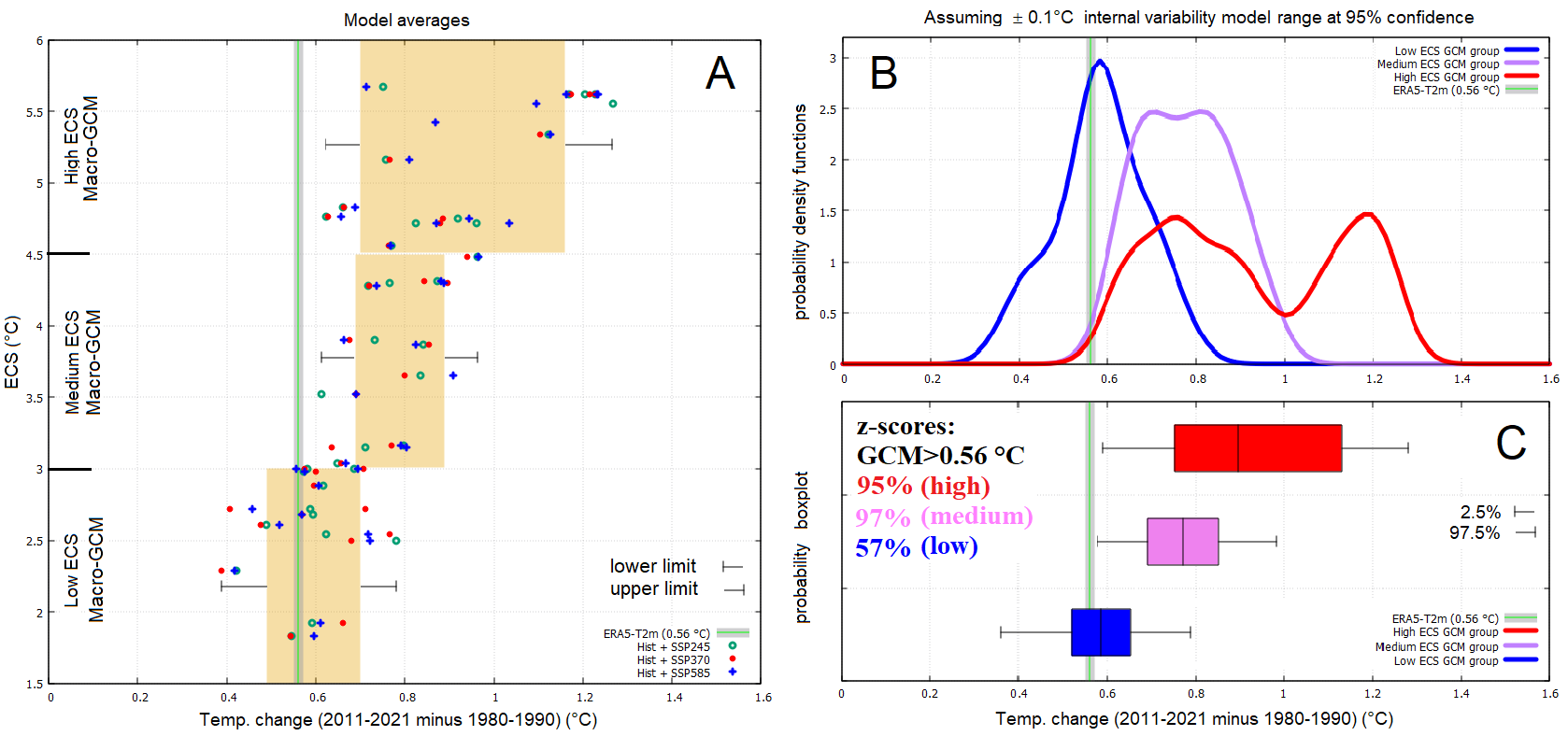
Figure 2: [A] Graphical reproduction of Table 1 in Scafetta (2022) showing three average hindcasts (blue, red and green dots) for each of 38 models. The yellow boxes represent the $\mu_{GCM}\pm\sigma_{GCM}$ range of the three macro-GCM distributions ($0.93\pm 0.22$, $0.77\pm 0.10$ and $0.58\pm 0.10$ °C) with whiskers representing their extremes. [B] Probability density functions (pdfs) for the Low-, Medium- and High-ECS macro-GCMs assuming a $\sigma_{95\%}=0.10\;{{}^{\circ}}\mathrm{C}$ additional dispersion from each model average to simulate the GCM internal variability. [C] Boxplots ($2.5\%,\;25\%,\;50\%,\;75\%,\;97.5\%$) for the pdfs in B with their z-scores. The green vertical line represents the estimated ERA5-T2m warming (Jan/2011–June/2021 mean) with a $\pm 0.01\;{{}^{\circ}}\mathrm{C}$ statistical error ($\pm\sigma$).

The z-score is for $z=(\mu_{obs}-\mu_{GCM})/\sqrt{\sigma_{obs}^{2}+\sigma_{GCM}^{2}+0.05^{2}}$, where $\mu_{obs}=0.56$ is the observed temperature mean, $\mu_{GCM}$ is the macro-GCM-hindcast-distribution mean, $\sigma_{obs}^{2}=0.01^{2}$ is the data variance, $\sigma_{GCM}^{2}$ is the macro-GCM variance and $0.05^{2}$ is the assumed additional variance related to each GCM internal variability.

Indeed, when a set of GCMs with comparable ECS properties is evaluated as a macro-GCM, as done in S2022, even if a few models or some of their simulations roughly hindcasted the observation (as some black dots shown in Figure 1 do) it would not demonstrate that the macro-GCM performs well as a whole. In order to compare the actual data with the macro-GCM hindcasts, statistical analyses like those shown in Figure 2 are required.

Here, I’m only concerned with the 11-year uncertainty of one record, not the uncertainty resulting from variations among different temperature records. In any case, all available global surface temperature records show a 1980–1990 to 2011–2021 warming between 0.52 and $0.59\;{{}^{\circ}}\mathrm{C}$ (Scafetta, 2023a), which could also be significantly overestimated according to alternative climatic records (Scafetta, 2023a, b; Spencer et al., 2017; Zou et al., 2023). The real 2011–2021 warming could be 0.4-0.6 °C, which is well-below the Medium- and High-ECS macro-GCM distrubutions.

Scafetta (2023b) proposed an ideal macro-GCM composed of 17 GCMs (from a collection of 41 GCMs) by selecting the top-performing models based on their ECS and transient climate response (TCR) rankings. Because of their low TCR, certain medium and high ECS models could be added to the low-ECS category in this situation.

5 The Areal Student t-test Analysis

SJK2023 also critiqued the second analysis that S2022 proposed, which was based on areal t-test statistics. The analysis was based on this equations:

$$\Delta T_{j}=\frac{1}{N}\sum_{i=1}^{N}\Delta T_{i,j}^{m}-\Delta T_{j}^{o};\qquad t_{j}=\frac{\left|\Delta T_{j}\right|}{\sigma_{j}/\sqrt{N}},$$ (18)

where $j=1,...,M$ are the grid cells, $i=1,...,N$ are the models, $t_{j}$ represents the Student t-test variable and $\sigma_{j}$ is the standard deviation of the distribution of the GCM hindcasts: $m$ indicates “model”, and $o$ indicates “observation”. SJK2023 claimed that $\sqrt{N}$ should be replaced by 1.

SJK2023 did not propose a “more appropriate test” but only a complementary one that does not change the conclusion of S2022 that, as the ECS lowers, the agreement between model hindcasts and actual observations increases, on average, also at the local scale (Scafetta, 2022, figure 5). In fact, S2022’s areal Student t-test maps can just be rescaled by $1/\sqrt{N}$ if a reader is interested in studying the alternative analysis. The test without $\sqrt{N}$ was adopted for the global scale (Figure 2) where a dynamical comparison among the various regions was not needed.

It is perplexing why SJK2023 asserted that the Student t-test would not be adequate for evaluating the performance of the climate models given that it is a well-known and reliable statistical instrument of analysis. The major goal was to assess the local performance of the three macro-GCMs. If $N$ increases, the rejection rate would only rise if the models’ reconstruction of the temperature changes exhibited a systematic bias. In fact, for reliable models, the mean divergence from the observed values should converge to zero ($\left|\Delta T_{j}\right|\rightarrow 0$) quicker than $1/\sqrt{N}$, and Eq. 18 will keep $t$ small ($t\rightarrow 0$). Additionally, the (rather weak) dependence of the t-test equation on $N$ can be easily solved by standardizing the proposed test by using always a fixed number of models (e.g., $N=10$ or other), and, if necessary, averaging the areal t-test results among these subsets.

In fact, the GCMs should hindcast the primary dynamical patterns produced by the climate system, including those generated by the global atmospheric and oceanic circulation. The fact that they cannot do it yet, does not invalidate Eq. 18. Simple energy balance models might just replace the GCMs if they were not intended to reconstruct the global circulation even at a timescale larger than the decadal one. S2022’s test successfully brought attention to the persistent problems in climate dynamics that need to be solved in order to improve the models.

On the other side, the “more appropriate test” proposed by SJK2023 would be inadequate for detecting specific dynamical biases in the model ensemble because, for instance, one GCM simulation might accurately reproduce the warming over China but not over Africa, whereas another simulation might accurately reproduce the warming over Africa but not over China (and so on). If the scaling provided by the factor $\sqrt{N}$ in Eq. 18 is not used, and the two simulations are just superimposed, the analysis would give the false impression that the GCM reconstructs the temperatures in both China and Africa, which would be misleading because none of the actual simulations would do it.

S2022’s recommended test is stringent, but statistical tests are generally more useful when they reveal physical inconsistencies rather than when they cover them under the umbrella of large stochastic error-bands.

6 Conclusion

SJK2023 made an incorrect use of statistics and physics because they evaluated $\sigma_{\mu}$ of 11 different annual temperatures by using the SDOM of a (here-nonexistent) distribution of one quantity instead of the GEPF of a N-quantity function like the “mean”, and confused natural interannual chaotic variability with random noise.

Statistical equations only apply to the stochastic component of a signal, not to its physical one, which is regulated by the laws of physics. The uncertainty of any function of a temperature chronology (such as its mean) arises only from the stochastic errors of the data-points and their error-covariance (Eq. 5). Whether the El-Niño fluctuations are caused by internal mechanisms or external forcings, or how well they can be predicted by modern GCMs, is irrelevant for calculating the data errors at the decadal or any other timescale. The observational errors must not be confused with the errors of the regression parameters of a model-interpretation of the data.

More specifically, SJK2023 inflated the error of the ERA5-T2m 2011–2021 mean by 5–10 times by confusing it with the error of the regression parameter $M$ of an isothermal climate model that postulates that the interannual temperature variability is random noise, which is nonphysical. Their $\sigma_{\mu,95\%}\approx 0.10\,{{}^{\circ}}\mathrm{C}$ 11-year error-estimate is contradicted by published temperature data (e.g. Figure 1C) and was also arbitrarily calculated using annual average values, as opposed to monthly ones, which produce with Eq. 1 a very different result, $\sigma_{\mu,95\%}\approx 0.03\,{{}^{\circ}}\mathrm{C}$.

Additionally, SJK2023 ignored that S2022’s main result was confirmed by three different sets (one for each SSP) of GCM average simulations and that S2022’s primary goal was to test three macro-GCMs characterized by different ECS ranges. Finally, Scafetta (2023a) answered all of SJK2023’s questions about the hindcast uncertainty of the models and confirmed that the most likely ECS should be lower than 3 °C, as Figure 2, which complements S2022, shows once again.

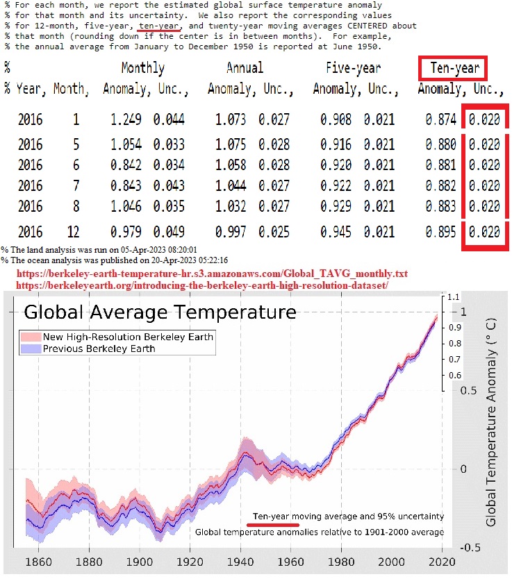
Figure 3: Berkeley Earth global average temperature, decadal scale with its 95% uncertainty range, which after 1980 is about $\pm 0.02$ °C.

References

- Bose (2021) Bose, S. (2021). Error Propagation Calculator. Available at: https://astro.subhashbose.com/tools/error-propagation-calculator (accessed on June 04, 2023).
- Craigmile and Guttorp (2022) Craigmile, P. F., Guttorp, P. (2022). A combined estimate of global temperature. Environmetrics, 33:e2706 https://doi.org/10.1002/env.2706
- Hausfather et al. (2022) Hausfather, Z., Marvel, K., Schmidt, G.A., Nielsen-Gammon, J.W., Zelinka, M. (2022). Climate simulations: recognize the ‘hot model’ problem. Nature, 605, 26–29. https://doi.org/10.1038/d41586-022-01192-2
- Hersbach et al. (2020) Hersbach, H., Bell, B., Berrisford, P., et al. (2020). The ERA5 global reanalysis. Quaternary Journal of the Royal Meteorological Society 146, 1999–2049. https://doi.org/10.1002/qj.3803. See also the voice “(9) Where can I find monthly-mean values for uncertainty? There are NO monthly mean values for uncertainties available” in https://confluence.ecmwf.int/display/CKB/ERA5%3A+uncertainty+estimation (accessed on June 04, 2023).
- JCGM (2008) JCGM member organizations (BIPM, IEC, IFCC, ILAC, ISO, IUPAC, IUPAP and OIML). Evaluation of measurement data — Guide to the expression of uncertainty in measurement. Joint Committee for Guides in Metrology, JCGM 100:2008. URL: https://www.bipm.org/documents/20126/2071204/ JCGM_100_2008_E.pdf/cb0ef43f-baa5-11cf-3f85-4dcd86f77bd6 (accessed on June 04, 2023).
- Lafarge and Possolo (2015) Lafarge, T., Possolo A. (2015). The NIST Uncertainty Machine. NCSLI Measure Journal of Measurement Science, 10(3), 20–27. Available at: https://uncertainty.nist.gov/ (accessed on June 04, 2023).
- Lessen et al. (2019) Lenssen, N.J.L., Schmidt, G.A., Hansen, J.E., et al. (2019) Improvements in the GISTEMP uncertainty model. Journal of Geophysical Research: Atmospheres 124:6307–6326. https://doi.org/10.1029/2018JD029522
- Lewis (2023) Lewis, N. (2023). Objectively combining climate sensitivity evidence. Climate Dynamics 60, 3139–3165 https://doi.org/10.1007/s00382-022-06468-x
- Morice et al. (2021) Morice, C.P., Kennedy, J.J., Rayner, N.A., et al. (2021). An updated assessment of near-surface temperature change from 1850: the HadCRUT5 data set. Journal of Geophysical Research: Atmospheres 126, e2019JD032361. https://doi.org/10.1029/2019JD032361
- Rohde et al. (2020) Rohde, R.A., Hausfather, Z. (2020). The Berkeley Earth Land/Ocean Temperature Record. Earth Syst. Sci. Data 12, 3469–3479. https://doi.org/10.5194/essd-12-3469-2020. Monthly global average temperature file: https://berkeley-earth-temperature.s3.us-west-1.amazonaws.com/Global/Land_and_Ocean_complete.txt (accessed on June 04, 2023).
- Scafetta (2022) Scafetta, N. (2022). Advanced testing of low, medium, and high ECS CMIP6 GCM simulations versus ERA5-T2m. Geophysical Research Letters, 49, e2022GL097716. https://doi.org/10.1029/2022GL097716.
- Scafetta (2023a) Scafetta, N. (2023a). CMIP6 GCM ensemble members versus global surface temperatures. Climate Dynamics 60, 3091–3120. https://doi.org/10.1007/s00382-022-06493-w
- Scafetta (2023b) Scafetta, N. (2023b). CMIP6 GCM Validation Based on ECS and TCR Ranking for 21st Century Temperature Projections and Risk Assessment. Atmosphere, 2023, 14, 345. https://doi.org/10.3390/atmos14020345
- Schmidt et al. (2022) Schmidt, G.A., Jones, G.S., Kennedy, J.J.: Issues and Errors in “Advanced Testing of Low, Medium, and High ECS CMIP6 GCM Simulations Versus ERA5-T2m” by N. Scafetta (2022). Real Climate, 30 March 2022, 2022. https://www.realclimate.org/images//Issues_with_Scafetta_2022v2.pdf (accessed on June 04, 2023).
- Schmidt (2022) Schmidt, G.A.: Scafetta comes back for more. Real Climate, 10 October 2022. https://www.realclimate.org/index.php/archives/2022/10/scafetta-comes-back-for-more/ (accessed on June 04, 2023).
- Schmidt et al. (2023) Schmidt, G.A., Jones, G.S., Kennedy, J.J. (2023). Comment on “Advanced Testing of Low, Medium, and High ECS CMIP6 GCM Simulations Versus ERA5-T2m” by N. Scafetta (2022). Geophysical Research Letters, 50, e2022GL102530. https://doi.org/10.1029/2022GL102530
- Sherwood et al. (2020) Sherwood, S.C., Webb, M.J., Annan, J.D., Armour, K.C., Forster, P.M., Hargreaves, J.C., et al. (2020). An assessment of Earth’s climate sensitivity using multiple lines of evidence. Reviews of Geophysics, 58, e2019RG000678. https://doi.org/10.1029/2019RG000678
- Spencer et al. (2017) Spencer, R.W., Christy, J.R., Braswell, W.D. (2017). UAH version 6 global satellite temperature products: Methodology and results. Asia-Pacific Journal of the Atmospheric Sciences, 53(1), 121–130. https://doi.org/10.1007/s13143-017-0010-y
- Taylor (1997) Taylor, J.R. (1997). An Introduction to Error Analysis: The Study of Uncertainties in Physical Measurements (second edition). University Science Books.
- Wienand (2019) Wienand, J. (2019). Error Propagation Calculator. Available at http://www.julianibus.de/ (accessed on June 04, 2023).
- Zou et al. (2023) Zou, C.-Z., Xu, H., Hao, X., Liu, Q. (2023). Mid-tropospheric layer temperature record derived from satellite microwave sounder observations with backward merging approach. Journal of Geophysical Research: Atmospheres, 128, e2022JD037472. https://doi.org/10.1029/2022JD037472