Advancing Parsimonious Deep Learning Weather Prediction using the HEALPix Mesh

Abstract

We present a parsimonious deep learning weather prediction model on the Hierarchical Equal Area isoLatitude Pixelization (HEALPix) to forecast seven atmospheric variables for arbitrarily long lead times on a global approximately 110 km mesh at 3h time resolution. In comparison to state-of-the-art machine learning weather forecast models, such as Pangu-Weather and GraphCast, our DLWP-HPX model uses coarser resolution and far fewer prognostic variables. Yet, at one-week lead times its skill is only about one day behind the state-of-the-art numerical weather prediction model from the European Centre for Medium-Range Weather Forecasts. We report successive forecast improvements resulting from model design and data-related decisions, such as switching from the cubed sphere to the HEALPix mesh, inverting the channel depth of the U-Net, and introducing gated recurrent units (GRU) on each level of the U-Net hierarchy. The consistent east-west orientation of all cells on the HEALPix mesh facilitates the development of location-invariant convolution kernels that are successfully applied to propagate global weather patterns across our planet. Without any loss of spectral power after two days, the model can be unrolled autoregressively for hundreds of steps into the future to generate stable and realistic states of the atmosphere that respect seasonal trends, as showcased in one-year simulations. Our parsimonious DLWP-HPX model is research-friendly and potentially well-suited for sub-seasonal and seasonal forecasting.

1 Introduction

Four years ago, Weyn et al. (2019) posed the question “Can machines learn to predict the weather?” and demonstrated that data driven convolutional neural networks can forecast the evolution of the 500- surface much better than the alternative dynamical model, the barotropic vorticity equation, which was used in the first numerical weather prediction (NWP) model (Charney et al., 1950). An extremely rapid evolution of deep learning weather prediction (DLWP) models followed, culminating in the recent Pangu-Weather (Bi et al., 2023) and GraphCast models (Lam et al., 2022), which outperform the state-of-the-art Integrated Forecast System (IFS) of the European Centre for Medium-Range Weather Forecasts (ECMWF) according to numerous metrics.

NWP has continuously improved over the seven decades since the first barotropic model forecast (Benjamin et al., 2019). Current state-of-the-art models typically provide skillful predictions of global weather patterns at effective grid point spacings of roughly $0.1\text{\,}{}^{\circ}$ of latitude (about $10\text{\,}\mathrm{k}\mathrm{m}$) through at least seven days of forecast lead time (Bauer et al., 2015). The computational effort required to generate such global high-resolution forecasts is enormous and only available at a handful of advanced dedicated centers. Ensemble forecasts, which provide an important way to account for uncertainty by generating a set of equally plausible predictions and extend the limit of skillful forecasts beyond that of a single deterministic model run, are also limited by the computational burden of high-resolution NWP to about 50 members (Palmer, 2019).

Global NWP models represent 3D fields as sets of nested spherical shells in which the distance between each shell is the local vertical grid spacing. On every time step, the ECMWF Integrated Forecasting System (IFS), as configured for sub-seasonal forecasting, updates 9 prognostic 3D variables defined at 91 vertical levels. Along with surface pressure, this totals to 820 spherical shells of data. Here, we use “spherical shell of data” to describe a single variable defined at a single vertical level on a spherical shell covering the globe. The large number of spherical shells of data (combined with the fine horizontal resolution) in NWP models is required to produce acceptably accurate numerical solutions to the equations governing atmospheric motions. The data at each individual point, however, cannot be independently perturbed while maintaining a meteorologically relevant atmospheric state. For example, on horizontal scales larger than about $10\text{\,}\mathrm{k}\mathrm{m}$, the temperatures throughout a vertical column and the heights of constant pressure surfaces must satisfy hydrostatic balance.

The actual number of independent degrees of freedom required to represent the predictable components of the global atmosphere is unknown, but it clearly decreases with increasing forecast lead times (Lorenz, 1969). GraphCast (Lam et al., 2022), for example, has achieved success at lead times as short as $6\text{\,}\mathrm{h}$ with 227 spherical shells of data. It can produce forecasts using much less computation time than the ECMWF IFS, but it still requires large computing resources for training: 3 weeks using 32 TPU 4 processors. Pangu-Weather (Bi et al., 2023) cuts the number of spherical shells by almost 2/3 to 69. Here, we take this reduction much farther, presenting a parsimonious DLWP model that uses just 7 spherical shells of data to efficiently provide forecasts approaching the skill of ECMWF. While not as accurate as GraphCast or Pangu-Weather, our model is potentially better suited for research applications requiring a simpler model or focusing on long-lead time forecasts (e.g., sub-seasonal).

In addition to producing reasonably accurate deterministic forecasts, our new DLWP-HPX model can be stepped forward to a full year without becoming unstable or gradually smoothing toward climatology. In contrast to many of the recent DLWP architectures, our approach relies on convolutional neural networks (CNN), building on early work by Scher and Messori (2018) and Weyn et al. (2019) and the U-Net configuration in Weyn et al. (2020) and Weyn et al. (2021). Here, we document substantial improvements over Weyn et al. (2021), obtained by replacing the cubed sphere data representation with the HEALPix mesh, which is widely employed in astronomy (Gorski et al., 2005). In addition, we improve the former model by implementing physically motivated modifications in form of residual connections, recurrent modules, and inverting the channel depth as compared with a standard U-Net.

2 Related Work

Pioneering efforts to create machine learning models to forecast the weather from reanalysis or general circulation model (GCM) output include the dense neural network of Dueben and Bauer (2018) and the CNN models of Scher and Messori (2019) and Weyn et al. (2019), all of which employed latitude longitude (lat-lon) meshes. Weyn et al. (2020) obtained significantly improved forecasts by switching to a cubed sphere mesh with a CNN in the standard U-Net architecture (Ronneberger et al., 2015). Their model was capable of generating realistic weather patterns when stepped forward for a full year (730 $12\text{\,}\mathrm{h}$ steps). Retaining the cubed sphere, Weyn et al. (2021) produced forecasts out to sub-seasonal time scales using large multi-model ensembles, and Lopez-Gomez et al. (2022) migrated from the U-Net into a U-Net 3+ architecture (Huang et al., 2020) to generate forecasts of extreme surface temperatures.

Returning to the lat-lon mesh, Rasp and Thuerey (2021) demonstrated that a deep Resnet could be pre-trained on GCM data and then fine-tuned by transfer learning on ERA5 data to produce up to 5-day forecasts at coarse $5.65\text{\,}{}^{\circ}$ grid spacing. Building on transformer models from computer vision (Dosovitskiy et al., 2020; Guibas et al., 2021), Pathak et al. (2022) and Kurth et al. (2022) used Fourier neural operators (Li et al., 2020) to develop FourCastNet on a $0.25\text{\,}{}^{\circ}$ lat-lon mesh to generate forecasts approaching the accuracy of ECMWF’s IFS. FourCastNet was not, however, capable of stable long-lead-time autoregressive rollouts. This difficulty was overcome by switching from 2D Fourier modes on a lat-lon mesh to spherical harmonic functions Bonev et al. (2023). The resulting SFNO model eliminated much of the vision transformer architecture while improving accuracy and remaining stable for one-year forecasts.

Again on a 5.65^∘ lat-lon mesh, Hu et al. (2022) used a shifted window (Swin) transformer (Liu et al., 2021) to produce single forecasts as well as ensembles generated by perturbing the latent state using samples from their learned distribution. Bi et al. (2023) also applied Swin transformers on a lat-lon mesh, but used a fine $0.25\text{\,}{}^{\circ}$ lat-lon grid spacing, 3D transformers, and included latitude and longitude fields as input to train a “3D Earth-specific transformer” at four different forecast lead times of $1\text{\,}$, $3\text{\,}$, $6\text{\,}$, and $24\text{\,}\mathrm{h}$, which are used in combination to span an arbitrary hourly forecast period with minimal model steps. If the ECMWF IFS NWP forecasts are averaged to the coarser $0.25\text{\,}{}^{\circ}$ lat-lon mesh, Pangu-Weather outperforms NWP on several metrics.

In contrast to the preceding approaches, graph neural networks (Gori et al., 2005; Scarselli et al., 2008; Kipf and Welling, 2016; Battaglia et al., 2018; Pfaff et al., 2020) where applied on icosahedral meshes at course resolution by Keisler (2022) and at fine resolution in the Graphcast model (Lam et al., 2022). Similarly to Pangu-Weather, GraphCast appears to outperform the coarsened ECMWF IFS forecast on several metrics.

3 Methods

3.1 Data

3.1.1 Choice of Variables

Beginning with the same six prognostic variables used in Weyn et al. (2021)—geopotential height at $1000\text{\,}\mathrm{h}\mathrm{P}\mathrm{a}$ and $500\text{\,}\mathrm{h}\mathrm{P}\mathrm{a}$ ($Z_{1000}$, $Z_{500}$), $700\text{\,}\mathrm{h}\mathrm{P}\mathrm{a}$ to $300\text{\,}\mathrm{h}\mathrm{P}\mathrm{a}$ thickness ($\tau_{700-300}$) defined as $Z_{300}-Z_{700}$, temperature at $2\text{\,}\mathrm{m}$ height above ground ($T_{2m}$), temperature at $850\text{\,}\mathrm{h}\mathrm{P}\mathrm{a}$ ($T_{850}$), and total column water vapor ($TCWV$)—we add $Z_{250}$ based on its importance in the model of Rasp and Thuerey (2021) and to provide an upper tropospheric variable. As in Weyn et al. (2021), three prescribed fields are also provided: topographic height, land-sea mask, and top-of-atmosphere (TOA) incident solar radiation. No specific information about position on the globe, such as latitude and longitude, is provided. Three-hourly data from the ERA5 reanalysis (Hersbach et al., 2020) provide training data from 1979-2012, a validation set from 2013-2016, and a test set from 2017-2018.

3.1.2 HEALPix Mesh

We discretize all fields using the Hierarchical Equal Area isoLatitude Pixelization (HEALPix) (Gorski et al., 2005). As depicted in Figure 1, a HEALPix mesh is formed by dividing the sphere into twelve equal-area diamond-shaped faces, with four faces lying in the northern and southern hemispheres, and four in the tropics. According to Gorski et al. (2005), the HEALPix mesh has three important properties. (1) Hierarchical structure of the database: Each of the twelve base faces can be progressively subdivided into smaller patches. (2) Equal areas for the discrete elements of the partition: All patches are the same size. (3) Isolatitude distribution for the discrete area elements on the sphere: The patches line up with lines of latitudes, facilitating the computation of zonal averages and one-dimensional zonal spectra. Importantly, this last property makes the HEALPix mesh an “east is to the right” grid, which facilitates the training of CNN kernels to capture the motion of typical weather disturbances, as discussed in Section 4.1.

The HEALPix can be considered a graph and does not allow a seamless application of convolution operations. Thus, Perraudin et al. (2019) explicitly define a graph from the HEALPix—by connecting adjacent neighbors with weighted edges—and perform a graph convolution to classify weak lensing maps from cosmology. In a different approach, Krachmalnicoff and Tomasi (2019) classify digits and determine cosmic parameters from simulated cosmic microwave background maps. They apply 1D convolutions to the flattened HEALPix data with a kernel size $k$ and stride $s$ both equal to 9, appending a zero to those cases where only seven instead of eight neighbors are defined (top corner of the tropical faces). In contrast, we treat the twelve faces as distinct images and pad their boundaries using data from neighboring faces to allow the computation of 2D convolutions and averaging operators directly, as detailed in Appendix A. To accelerate the padding operation, we have implemented a custom CUDA kernel, which is available in our repository.

The grid spacing, or shortest inter-node spacing, on the HEALPix mesh is the diagonal distance between a pair of nodes on adjacent latitude lines. Denoting a HEALPix mesh with $n$ divisions along one side of the original 12 faces as HPX$n$. The grid spacing is approximately 220 km ($\approx 2{{}^{\circ}}$) for HPX32 and 110 km ($\approx 1{{}^{\circ}}$) for HPX64.

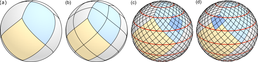
Figure 1: Division of the sphere into twelve faces according to the HEALPix. Four faces to represent either the northern (blue) and southern extratropics, while four more faces arrange around the equator to represent the tropics (yellow). Each face can be subdivided into patches with divisions along the side of each face given by powers of two. The sphere in (a) has a pixel-count of one per face side; we call it hpx1. The sphere in (b) counts two pixels per side (hpx2), whereas the two spheres in (c) and (d) have eight pixels per side, i.e., hpx8. Several latitude lines in red emphasize the iso-latitudinal arrangement of the patches. The saturated blue area depicts a $3\times 3$ stencil, as applied by a standard convolution. To apply the $3\times 3$ stencil at the top corner of the equatorial faces, i.e., stencil position in (d), we simulate a hypothetical patch by computing the average from the according extratropical face patches.

3.2 Machine Learning Architecture

Relating to Tobler’s first law of geography: “All things are related, but nearby things are more related than distant things.” (Tobler, 1970), we mostly retain the comparably simple U-Net structure from Weyn et al. (2020). U-Nets (Ronneberger et al., 2015) are hierarchically structured feed-forward convolutional neural networks that were originally proposed for segmenting biomedical images. The U-Net structure proposed here introduces several physically motivated advancements to the vanilla U-Net used by Weyn et al. (2021) for time-series forecasting. The advancements are visualized in Figure 2, detailed in Table 1, and described in the following.

3.2.1 Residual Prediction

We switch to a residual prediction approach both for the full predictive step and within each ConvNeXt block. Predicting changes over a time step, instead of the full fields, is similar to the discretization of time derivatives when solving partial or ordinary differential equations, and has been used successfully in previous deep-learning weather prediction models (Pathak et al., 2022; Keisler, 2022; Hu et al., 2022; Lam et al., 2022).

3.2.2 Inverting the Ordering of Channel Depth

The standard U-Net for semantic segmentation (Ronneberger et al., 2015) and its successors (Zhou et al., 2018; Huang et al., 2020) employ relatively few channels on the highest level and successively double the channel depth, while halving the spatial resolution in each deeper layer. This ordering is useful in image segmentation tasks, where deeper channels are required to create increasingly abstract filters to identify semantic features and express complex objects. In weather prediction, however, we find it is better to devote more capacity to the layers in the first level, where a wide variety of fine grained weather phenomena must be captured. Deeper layers at coarser resolution, on the other hand, need only encode larger scale atmospheric motions, which can be adequately represented with comparably fewer channels.

Thus, we invert the channel order, employing 136, 68, and 34 channels in each convolution on the first, second, and third layer, respectively (cf. Figure 2). While this modification improves the model performance significantly, it also increases the computational burden, since more computations and data processing are required to evaluate the additional convolutions at fine spatial resolution. Tests which preserved the total number of trainable parameters, but completely eliminated the deeper layers in the U-Net gave worse results, demonstrating that the longer-range connections and richer latent space structures enabled by the full U-Net architecture remain important.

3.2.3 Recurrent Modules

The vanilla U-Net is a feed-forward network, which treats successive inputs independently even if the data represents a continuous sequence over time. Feed-forward networks do not have any memory capacity. They do not maintain an internal state between time steps. To enable the exploitation of information from previous latent states, we include a gated recurrent unit (GRU) (Cho et al., 2014) at the end of each decoder block with kernel size $k=1$. We chose GRUs over LSTMs (Hochreiter and Schmidhuber, 1997) since we re-initialize the recurrent data over each $24\text{\,}\mathrm{h}$-cycle, and therefore do not require forget-gates (as confirmed experimentally, not shown).

3.2.4 Miscellaneous Modifications

Several other components of the original Weyn et al. (2021) model were modified based on recent results from deep learning research: the capped leaky ReLU was replaced by capped GELU activations (Hendrycks and Gimpel, 2016); upsampling was changed from knn-interpolation to a transposed convolution; finally, the pairs of two successive convolutions were replaced at each encoder and decoder level in the U-Net by a modified ConvNeXt block (Liu et al., 2022), as visualized in Figure 2.

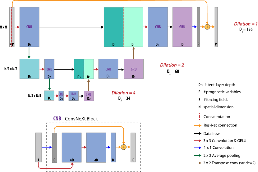
Figure 2: Schematic representation of the DLWP-HPX architecture for our best performing model. There is one ConvNeXt block at each level in both the encoder and the decoder. In contrast to the configuration in typical image processing applications, the channel, or latent-layer, depth decreases from 136 to 68 to 34 at deeper layers in the U-Net.

Table 1: Configuration and parameter counts of all layers in our best performing model, where $c_{\operatorname{in}}$ denotes the number of input channels, $k$ is the kernel size, $s$ the stride, and $d$ the dilation. The receptive field of each layer with respect to the network input is reported under RF and the output shape takes (F, H, W, C) with F the number of faces, H and W height and width, and C the number of output channels. The dashed line separates the model’s encoder (above) and decoder (below) components. All ConvNeXt- and GRU-blocks are additionally broken down into their operations, visualized by the indented layer names. Numbers in brackets following individual layer names correspond to outputs, which are concatenated to the respective Concat layers in the decoder. All convolution layers with $k=3$ are followed by GELU activation functions. Residual connections are not reported as they neither change the spatial resolution nor the number of channels, and they do not contribute to the parameter count. Color codes approximate those used in the model schematic in Figure 2.

							Parameter count
Layer	$c_{\operatorname{in}}$	$k$	$s$	$d$	RF	Output shape	Weights	Biases	$\Sigma$
ConvNeXt
Conv2d	018	1	1	1	$1\times 1$	(12, 64, 64, 136)	2 448	136	2 584
Conv2d	018	3	1	1	$3\times 3$	(12, 64, 64, 544)	88 128	544	88 672
Conv2d	544	3	1	1	$5\times 5$	(12, 64, 64, 544)	2 663 424	544	2 663 968
Conv2d (1)	544	1	1	1	$5\times 5$	(12, 64, 64, 136)	73 984	136	74 120
AvgPool2d	136	2	2	—	$6\times 6$	(12, 32, 32, 136)	0	0	0
ConvNeXt
Conv2d	136	1	1	1	$6\times 6$	(12, 32, 32, 068)	9 248	68	9 316
Conv2d	136	3	1	2	$14\times 14$	(12, 32, 32, 272)	332 928	272	333 200
Conv2d	272	3	1	2	$22\times 22$	(12, 32, 32, 272)	665 856	272	666 128
Conv2d (2)	272	1	1	1	$22\times 22$	(12, 32, 32, 068)	18 496	68	18 564
AvgPool2d	068	2	2	—	$24\times 24$	(12, 16, 16, 068)	0	0	0
ConvNeXt
Conv2d	068	1	1	1	$24\times 24$	(12, 16, 16, 034)	2 312	34	2 346
Conv2d	068	3	1	4	$56\times 56$	(12, 16, 16, 136)	83 232	136	83 368
Conv2d	136	3	1	4	$88\times 88$	(12, 16, 16, 136)	166 464	136	166 600
Conv2d	136	1	1	1	$88\times 88$	(12, 16, 16, 034)	4 624	34	4 658
ConvNeXt
Conv2d	034	1	1	1	$88\times 88$	(12, 16, 16, 068)	2 312	68	2 380
Conv2d	034	3	1	4	$120\times 120$	(12, 16, 16, 136)	41 616	136	41 752
Conv2d	136	3	1	4	$152\times 152$	(12, 16, 16, 136)	166 464	136	166 600
Conv2d	136	1	1	1	$152\times 152$	(12, 16, 16, 068)	9 248	68	9 316
GRU
Conv2d	136	1	1	1	$152\times 152$	(12, 16, 16, 136)	18 496	136	18 632
Conv2d	136	1	1	1	$152\times 152$	(12, 16, 16, 068)	9 248	68	9 316
ConvTrans2d	068	2	2	1	$154\times 154$	(12, 32, 32, 068)	18 496	68	18 476
Concat (2)	—	—	—	—	—	(12, 32, 32, 136)	0	0	0
ConvNeXt
Conv2d	136	3	1	2	$154\times 154$	(12, 32, 32, 272)	332 928	272	333 200
Conv2d	272	3	1	2	$162\times 162$	(12, 32, 32, 272)	665 856	272	666 128
Conv2d	272	1	1	1	$170\times 170$	(12, 32, 32, 136)	36 992	136	37 128
GRU
Conv2d	272	1	1	1	$170\times 170$	(12, 32, 32, 272)	73 984	272	74 256
Conv2d	136	1	1	1	$170\times 170$	(12, 32, 32, 136)	36 992	136	37 128
ConvTrans2d	136	2	2	1	$171\times 171$	(12, 64, 64, 136)	73 984	136	74 120
Concat (1)	—	—	—	—	—	(12, 64, 64, 272)	0	0	0
ConvNeXt
Conv2d	272	1	1	1	$171\times 171$	(12, 64, 64, 136)	36 992	136	37 128
Conv2d	272	3	1	1	$173\times 173$	(12, 64, 64, 544)	1 331 712	544	1 332 256
Conv2d	544	3	1	1	$175\times 175$	(12, 64, 64, 544)	2 663 424	544	2 663 968
Conv2d	544	1	1	1	$175\times 175$	(12, 64, 64, 136)	73 984	136	74 120
GRU
Conv2d	272	1	1	1	$175\times 175$	(12, 64, 64, 272)	73 984	272	74 256
Conv2d	272	1	1	1	$175\times 175$	(12, 64, 64, 136)	36 992	136	37 128
Conv2d	136	1	1	1	$175\times 175$	(12, 64, 64, 014)	1 904	14	1 918
							9 816 752	6 066	9 822 818

3.2.5 Time Stepping Scheme

Similarly to Weyn et al. (2021), we apply a two-in-two-out mapping with a temporal resolution twice as fine as the actual time step. For example, two atmospheric states $3\text{\,}\mathrm{h}$ apart (each consisting of seven prognostic, along with three prescribed fields) are concatenated and input to the model, which generates a new pair of states, each characterising the atmosphere $6\text{\,}\mathrm{h}$ later in time. This strategy is observed to stabilize and accelerate the training, since the model receives additional information about the atmosphere’s rate of change and only has to be called half as often.

The frequency spectrum of atmospheric kinetic energy has a strong peak at $24\text{\,}\mathrm{h}$ because many circulations are modulated by solar heating. We therefore evaluate the training loss function as the mean squared error over a $24\text{\,}\mathrm{h}$ period. Tests in which the MSE was evaluated over multi-day periods tended to result in a model that gradually approached climatology over many recursive steps.

Training our model only over one daily cycle does mean that the recurrent states of the GRUs are not optimized for long rollouts. To prevent the explosion of recurrent states when generating long multi-day forecasts, we re-initialize the recurrent states every $24\text{\,}\mathrm{h}$ as illustrated in Figure 3 for a $12\text{\,}\mathrm{h}$ time step with $6\text{\,}\mathrm{h}$ resolution. For training or for the first step in a long forecast rollout, the model predicts $\smash{[\hat{s}_{(t+6)},\hat{s}_{(t+12)}]}$ from initial data $\smash{[{s}_{(t-6)},{s}_{(t)}]}$, and then in the subsequent step uses $\smash{[\hat{s}_{(t+6)},\hat{s}_{(t+12)}]}$ to predict $\smash{[\hat{s}_{(t+18)},\hat{s}_{(t+24)}]}$. But before this, the hidden states for the GRUs are initialized in a preliminary step by calling the model once with the state pair $\smash{[s_{(t-18)},s_{(t-12)}]}$ and a hidden state $h_{0}$ initialized with zeros. The resulting forecast for $\smash{[\hat{s}_{(t-6)},\hat{s}_{(t)}]}$ is discarded, but the hidden state $h_{1}$ is supplied to the GRU and paired with the actual initial data $\smash{[{s}_{(t-6)},{s}_{(t)}]}$ for the first step of the model. As shown by the bottom row in Figure 3, in a forecast rollout, the next day’s prediction begins by re-initializing the GRU starting with forecast values from one time step earlier and $h_{0}$ set to zero to obtain $h_{1}$. Note that since the GRU is re-initialized every day, there would be five model steps per day when using a $6\text{\,}\mathrm{h}$ time step (with $3\text{\,}\mathrm{h}$ data resolution).

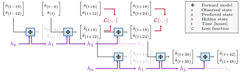
Figure 3: Two time-level input-output scheme with GRU for training and inference assuming $6\text{\,}\mathrm{h}$ time resolution. The output from the preliminary initialization step (light gray) is discarded, but the hidden state $h_{1}$ is generated and used in the first model step. The hidden state $h_{3}$ (light purple) at the end of the $24\text{\,}\mathrm{h}$ forecast is discarded as the GRU will be re-initialized for the next recursive inference step (lowest row). For training (top right), the loss function is computed from the four forecast times spanning $24\text{\,}\mathrm{h}$ period at $6\text{\,}\mathrm{h}$ resolution, as indicated in red.

3.2.6 Training

Our best performing DLWP-HPX model, described above, has $9.8\text{\,}\mathrm{M}$ parameters that are trained for 300 epochs (equivalent to 931,199 update steps) over eight days on four NVIDIA A100 GPUs with $80\text{\,}\mathrm{G}\mathrm{B}$ VRAM each. A batch size of eight per GPU is chosen, effectively resulting in an overall batch size of 32. We combine the Adam optimizer (Kingma and Ba, 2014) with a cosine annealing learning rate scheduler (Loshchilov and Hutter, 2016), setting the initial learning rate to $2\text{\times}{10}^{-4}\text{\,}$ and gradually refining it to zero. To stabilize the training, we clip the gradients to the current learning rate, which we observe to be particularly beneficial for large and recurrent models.

3.3 Courant-Friedrichs-Lewy Condition

Several leading DLWP models (Pathak et al., 2022; Hu et al., 2022; Bi et al., 2023; Chen et al., 2023) are based on Vision Transformers (ViTs) (Dosovitskiy et al., 2020), which were originally developed to account for non-local interactions in images; effectively working on patch embeddings. ViTs are successors of Transformers (Vaswani et al., 2017), which were introduced to efficiently accommodate very non-local interactions in natural language processing (NLP), where no fixed upper bound exists on the distance between words that may interact to change the meaning of a sentence. In contrast to ViTs, we use a U-Net to emphasize local interactions, where the Courant-Friedrichs-Lewy condition must be satisfied. To satisfy the condition, the fastest moving signal in the data must not exceed the maximum propagation speed that the model can reach when simulating the data.

There is a strong physical constraint on the locality of atmospheric interactions. That is, no information in the atmosphere travels faster than the speed of sound, roughly $300\text{\,}\mathrm{m}\mathrm{/}\mathrm{s}$. As a result, over a $12\text{\,}\mathrm{h}$ time step, sound waves travel roughly $13\,000\text{\,}\mathrm{k}\mathrm{m}$. Sound waves are not meteorologically significant, however. A better measure of the speed of the fastest moving signals of meteorological importance is the transport by the strongest jet-stream winds moving at roughly $100\text{\,}\mathrm{m}\mathrm{/}\mathrm{s}$, or about $4300\text{\,}\mathrm{k}\mathrm{m}$ in $12\text{\,}\mathrm{h}$.

The pair of 2$\times$2 average poolings and the dilations in the second and third levels of our U-Net architecture (Figure 2) substantially widen the receptive field that potentially influences the solution at a given point after each forward step of our model. Following terminology from numerical analysis, the receptive field could alternatively be termed the “numerical domain of dependence.” The Courant-Friedrichs-Lewy (CFL) condition—which is a necessary condition for convergence of numerical approximations to partial differential equations to the true solution of an associated set of governing equations—requires the numerical domain of dependence to include the domain of dependence of the true solution. Neglecting influences from special points at the corners of the twelve basic HEALPix faces, the receptive field at each stage of the neural network is listed in Table 1 and grows to a 175$\times$175 patch of cells after the last $3\times 3$ convolution in the decoder.

The diagonal distance between adjacent points on our 3$\times$3 stencil (dark blue patch in Figure 1) on a HPX64 mesh is approximately 110 . Thus, the receptive field for one step of our full HPX64 model is a patch exceeding $18\,900\text{\,}\mathrm{k}\mathrm{m}$ on each side, which is large enough to include all points influenced by sound wave propagation over a $12\text{\,}\mathrm{h}$ time step, and far more than would be required to contain the fastest moving meteorologically important signals. Note also that, at every step, our HPX64 forecast at a given point is influenced by a set of surrounding points containing roughly 70% of all the cells covering the globe.

4 Results

In the following, we first evaluate several key variables in our model over a 14-day forecast lead time, which is slightly longer than the period over which knowledge of the initial atmospheric conditions gives these single deterministic forecasts some predictive skill. We compare our best model with the ECMWF S2S forecasts and with our previous Weyn et al. (2021) results. We then document the successive improvements that our changes in model architecture have on the RMSE and ACC scores for $Z_{500}$. Next, we examine the ability of the model to distinguish between the amplitudes of the daily $T_{2m}$ ranges in tropical forests, in deserts, and over the ocean. Finally, we examine the behavior of the simulations over sub-seasonal (eight-week) and one-year free running rollouts.

4.1 Quantitative Performance Through 14-Day Forecast Lead Time

To compare our model with the results from Weyn et al. (2021) and to state-of-the-art NWP from ECWMF, we compute both root mean squared error (RMSE) between observations and model predictions and anomaly correlation coefficient (ACC) scores with respect to the ERA5 climatology. Both metrics are compared on a $1^{\circ}\times 1^{\circ}$ lat-lon mesh and weighted by latitude, requiring us to project our DLWP-HPX and Weyn et al. (2021) forecasts from the HEALPix and cube-sphere meshes onto the lat-lon grid. Because our ultimate focus is on sub-seasonal and seasonal forecasting, we compare against ECMWF’s integrated forecasting system for sub-seasonal forecasts (IFS S2S), which were initialized bi-weekly on Mondays and Thursdays and stepped forward at about $16\text{\,}\mathrm{k}\mathrm{m}$ effective resolution for the first 15 days (then doubling to $32\text{\,}\mathrm{k}\mathrm{m}$). For comparison with Weyn et al. (2021), our test set focuses on the years 2017 and 2018. Our computations are performed at HPX64 and $3\text{\,}\mathrm{h}$ resolution (corresponding to $6\text{\,}\mathrm{h}$ time steps). Key parameter attributes of the model from Weyn et al. (2021), IFS S2S, and our HPX64 model are listed in Table 2.

Table 2: Number of trainable parameters in millions, number of spherical shells of prognostic variables, horizontal resolution in degrees latitude, and temporal resolution ($\Delta_{t}$) of the models compared in Figure 4.

Model	Parameters	Spherical shells	Resolution	$\Delta_{t}$
Weyn 2021	2.7M	6	$1.4^{\circ}$	$6\text{\,}\mathrm{h}$
Our HPX64	9.8M	7	$1^{\circ}$	$3\text{\,}\mathrm{h}$
ECMWF	—	820	$0.15^{\circ}$	$0.2\text{\,}\mathrm{h}$

As shown in Figure 4, the RMSE scores for $Z_{500}$, 24-hour-averaged $T_{2m}$ (instantaneous $T_{2m}$ fields are not archived from the ECMWF S2S forecasts) and $T_{850}$ all improve substantially compared to Weyn et al. (2021). Moreover, despite the small number of prognostic variables and coarse spatial resolution of our model, the RMSEs for $Z_{500}$ and $T_{850}$ only lag the scores for ECMWF S2S by about 1 day at one-week lead time. As expected theoretically, the RMSE scores for all three models appear to be asymptotically approaching $\smash{\sqrt{2}}$ times climatology beyond two weeks when the skill of a single deterministic forecast drops toward zero. We present the comparison of 24-hour-averaged $T_{2m}$ between our model and IFS S2S for completeness, but it should be interpreted with caution. The re-gridding of both the IFS S2S and the HEALPix data to the $1^{\circ}\times 1^{\circ}$ lat-lon analysis grid introduces errors in the representation of coastlines and topography that significantly influence the surface temperature field. As a consequence, the RMSE values shown in Figure 4 (b) are not representative of those in each model’s native representation of the $T_{2m}$ field.

One additional issue that arises when plotting initial RMSE (and to a lesser extent ACC) for the ECMWF IFS S2S model is that, unlike our DLWP-HPX model, the IFS forecasts are not initialized with the ERA5 data. Thus, at very short forecast lead times, differences between the IFS initialization and the ERA5 data introduce apparent errors in the IFS forecast that are not representative of its actual performance. Lam et al. (2022) accounted for this in their comparison between the IFS and GraphCast, but it requires considerable extra computation. We are not claiming to outperform the IFS, so we simply suggest using caution when comparing errors between our models and the IFS at lead times less than 2 days.

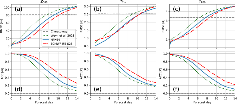
Figure 4: Comparison of the performance of the DLWP-HPX, Weyn et al. (2021), and ECMWF IFS S2S models, averaged over 208 forecasts. RMSE for (a) $Z_{500}$, (b) $T_{2m}$ and (c) $T_{850}$; climatology is indicated by the gray dashed line. ACC for or (d) $Z_{500}$, (e) $T_{2m}$ and (f) $T_{850}$.

ACC scores for $Z_{500}$, $T_{2m}$, and $T_{850}$ are also shown in Figure 4(d)–(f). As with RMSE, there is substantial improvement relative to both the previous model from Weyn et al. (2021) and the IFS S2S. In meteorological contexts, an ACC score of 0.6 is typically considered the lower limit of practical skill. The scores from our HEALPix model cross this threshold at about 7.5 days for $Z_{500}$ and 6.5 days for $T_{850}$, both of which are about 1.5 day sooner than the respective results for the IFS S2S. Numerical comparisons of the model RMSE and ACC scores averaged over the same 208 forecasts used to plot Figure 4 are given for 3-day and 5-day lead times in Table 3.

The relative importance of the various improvements in model architecture between Weyn et al. (2021) and our best DLWP-HPX model is illustrated for the $Z_{500}$ field in Figure 5. The total number of trainable parameters is held constant at roughly $2.7\times 10^{6}$ over the first five sets of changes. The RMSE rises to $50\text{\,}\mathrm{m}$ around 4.2 days in Weyn et al. (2021) (dark green dotted curve); replacing the $64\times 64$ cubed sphere by a HPX32 grid (aqua curve) delays the error growth by about 0.5 day despite the associated 50% reduction in total grid points. There is also a similar substantial improvement in the ACC. Continuing with the HPX32 mesh, we replace the capped ReLU by a capped GELU activation function, replace knn-interpolation by strided transposed convolution, and introduce dilated convolutions in the two lower levels of the U-Net (as detailed in Figure 2); this yields the modest but distinct improvements shown by the dark-blue curves.

Next, we replace the pairs of convolutions in each level of the encoder and decoder by a ConvNeXt block without a bottleneck (dashed tan curve). This actually produces a slight degradation in performance, but in other configurations closer to our final model, the ConvNeXt block does improve the performance, and importantly, it also reduces the memory footprint by about $25\%$ at a constant parameter count. A further significant improvement is obtained by inverting the standard U-Net progression in channel depth to have the most channels at the highest spatial resolution and the fewest at the lowest resolution (dark red curve). The final significant improvement in the 2.7-million parameter model is obtained by adding recurrence in the form of GRU cells in the decoder (green curve).

After adding the GRU cells, the rise of the RMSE to $50\text{\,}\mathrm{m}$ is delayed to about 5.3 days and the drop of the ACC below 0.6 to roughly 6.8 days. The next series of changes produces successive small improvements that push these values out to about 5.7 days for RMSE and 7.4 days for ACC. These improvements, as sequentially plotted in Figure 5, are: increasing the number of trainable parameters to $9.8\times 10^{6}$, adding the $Z_{250}$ field, increasing the horizontal resolution to HPX64 (which is more important for ACC than RMSE particularly on $T_{2m}$), and decreasing the time resolution to $3\text{\,}\mathrm{h}$. Benefits from the use of $3\text{\,}\mathrm{h}$ time resolution were only obtained if the model was configured with the GRUs.

Table 3: Root mean squared errors (RMSE) and anomaly correlation coefficient (ACC) scores for Weyn et al. (2021) (W21), our HPX64, and ECMWF’s IFS models, evaluated on geopotential at $500\text{\,}\mathrm{h}\mathrm{P}\mathrm{a}$ ($Z_{500}$), temperature $2\text{\,}\mathrm{m}$ above ground ($T_{2m}$), and temperature at $850\text{\,}\mathrm{h}\mathrm{P}\mathrm{a}$ ($T_{850}$) on lead times of 3 and 5 days.

		$Z_{500}$			$T_{2m}$			$T_{850}$
	Lead time	W21	HPX64	IFS	W21	HPX64	IFS	W21	HPX64	IFS
RMSE	3 days	36.26	21.88	14.91	1.17	0.82	1.02	1.95	1.49	1.35
	5 days	59.01	41.91	31.30	1.67	1.27	1.27	2.83	2.28	1.96
ACC	3 days	0.90	0.96	0.98	0.84	0.92	0.91	0.84	0.91	0.94
	5 days	0.70	0.84	0.92	0.66	0.78	0.83	0.64	0.76	0.84

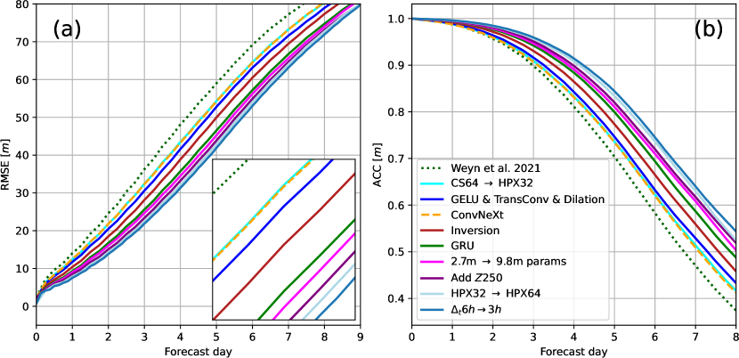
Figure 5: Impact of successive model improvements on the accuracy of $Z_{500}$ building from WDCC to our HPX64 model with $\Delta_{t}=$3\text{\,}\mathrm{h}$$. Each successive change builds on top of the previous architecture, adding the modification indicated in the legend: (a) RMSE, (b) ACC. Inset in (a) provides a magnified view of the error growth between 5 and 6 forecast days.

The single most effective modification in the preceding set of successive improvements is the migration from the cubed sphere to the HEALPix mesh, even though the $64\times 64$ cubed sphere has twice the total number of grid-points as the HPX32 mesh. The most likely explanation for the superiority of the HEALPix mesh is not simply that it is a more uniform covering of the globe than that provided by the cube-sphere, but that east and west have the same orientation in every HEALPix cell; we refer to this property as “east to the right.” In particular, the center and the east and west corners of each HEALPix cell are all at the same latitude. (A similar relationship holds in the north-south direction for meridians passing through those cells lying equatorward of the maximum north-south extent of the four equatorial faces in Figure 1 (a).) Thus, on the HEALPix mesh, eastward motion at all points and at all latitudes would be in the same direction across the diamond-shaped $3\times 3$ stencil in Figure 1 (c). In contrast, at any point on either of the polar faces on the cubed sphere, east could map to any of four directions along the axes of the $3\times 3$ convolutional stencil, depending on its longitude, as visualized in Appendix A.

In mid- and high-latitudes, most large-scale weather systems move in a generally eastward direction. We believe this allows a fixed number of kernel elements to more efficiently and effectively produce the required set of flow evolutions in the latent layers. To a lesser extent, this same consideration also applies to the four equatorial faces of the cubed sphere, where, for example, eastward flow near the northeastern corner of a face would need to move at an angle relative to the northern side of the stencil that is opposite in sign to that required in the northwestern corner.

4.2 Eliminating the Need for Boundary-Layer Parameterizations

Accurate forecasts of surface temperatures in NWP models rely on the empirical parameterization of multi-scale processes near the Earth’s surface in the atmospheric boundary layer (ABL). The bottom of the ABL includes the roughness layer (2–5 times the height of roughness elements such as vegetation), and the surface layer (often $10\text{\,}$–$100\text{\,}\mathrm{m}$ deep), where shear-driven turbulence dominates generation by convection. The depth of the full ABL, where larger-scale eddies and circulations communicate the processes in the surface layer to the free atmosphere, can vary from $O$(100) in calm stable nighttime conditions to several kilometers during the day over deserts.

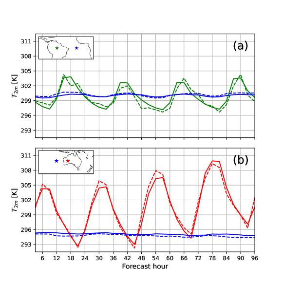
Figure 6: HPX64 simulation of the diurnal cycle of $T_{2m}$ (solid curves) at the four locations shown in the insets starting from 00 UTC on 12 March 2018. ERA5 values for the same $1^{\circ}\times 1^{\circ}$ lat-lon cell are shown as dashed lines. Values are plotted every 3 h.

No effort is made to explicitly account for ABL processes in our model; the $T_{2m}$ field is treated the same as the other six prognostic fields. The same CNN kernels are employed everywhere over the globe on the HEALPix mesh; the only data that might distinguish one location from another are the land-sea mask, the terrain elevation, and the TOA solar forcing; neither longitude nor latitude are provided. Yet our model does a good job of capturing the diurnal cycle in multi-day forecasts over very different surfaces. Figure 6 shows the diurnal cycle in $T_{2m}$ at locations over the Amazon forest, the Australian desert, and two adjacent oceans over a 4-day simulation starting at 00 UTC on 12 March 2018.

Compared to over land, the diurnal $T_{2m}$ variations are modest over the oceans, and they are well captured by our model. The land-sea mask is undoubtedly important in distinguishing the ocean locations from those over land. More interestingly, the model does an excellent job of capturing the large diurnal temperature range over the Australian desert, while correctly generating a much lower amplitude signal over the Amazon. The prognostic field that has most likely facilitated this distinction is $TCWV$, which is significantly higher over the Amazon than over the Australian desert. The model also captures the 4-day trend for increasing temperatures over Australia, which is linked to the evolution of larger-scale weather systems. Overall, the ability of the model to capture the diurnal $T_{2m}$ cycle with just seven prognostic fields, without any special treatment of the ABL, and without geo-specific inputs such as latitude and longitude is suggestive of the power and potential of DLWP-HPX.

4.3 Realistic Simulations Over Long Iterative Rollouts

To investigate the stability of our model when unrolling a forecast far into the future, we initialize it using ERA5 data for 00 UTC on 1 June 2017 (together with the 21 UTC fields on 31 May). Using $6\text{\,}\mathrm{h}$ time steps (with $3\text{\,}\mathrm{h}$ time resolution), we perform 1460 iterations to generate a 365-day forecast. The three-day running mean of $Z_{500}$, averaged around each latitude, is plotted as a function of latitude and time for a full year in Figure 7, along with the corresponding averages from the ERA5 data. Despite being trained to minimize RMSE over a single day and not enforcing any physical constraints, the DLWP-HPX simulation responds to the TOA solar forcing to generate the annual cycle reasonably well.

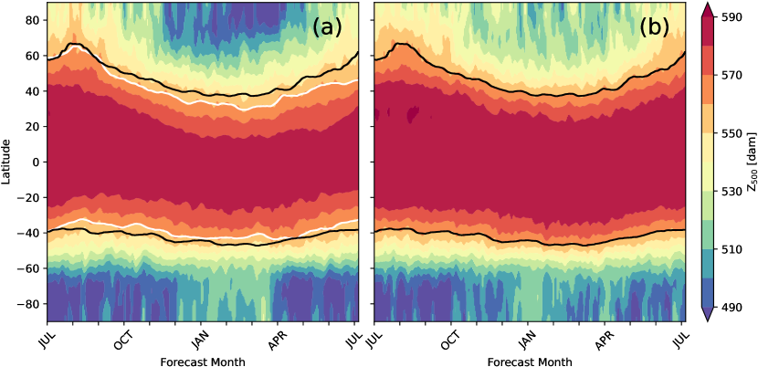
Figure 7: Zonally averaged three-day mean of $Z_{500}$ plotted as a function of time and latitude: (a) for a recursive one-year model simulation initialized on 1 July 2017, (b) the corresponding averaged $Z_{500}$ field from the ERA5 reanalysis. 15-day averaged values for the 560 dam contour for the ERA5 data (black line, both panels) and for the DLWP-HPX simulation (white line in (a)).

One region where the errors are significant is the arctic. About 5 months into the simulation, the simulated heights in the arctic region drop as much as $60\text{\,}\mathrm{m}$ below those in the reanalysis during the boreal winter. In contrast, at 5–8-month lead times, the heights in the antarctic region increase to approximately correct values in the austral summer.

There is also a long-term drift toward lower heights in the subtropics and mid-latitudes, creating a roughly $30\text{\,}\mathrm{m}$ loss in $Z_{500}$ by the end of the 1-year forecast. Climate models are tuned to avoid long-term drift in the predicted fields, but operational NWP models are not so tuned. For example, significant model biases that grow over a time scale of several weeks are removed to create sub-seasonal ECMWF IFS S2S forecasts (Vitart, 2004; Weigel et al., 2008). To facilitate comparison of model drift with the ERA5 reanalysis, the pair of black lines in both panels show the 15-day mean of the zonally averaged $560\text{\,}\mathrm{d}\mathrm{a}\mathrm{m}$ contours in the northern and southern hemisphere. The white lines in Figure 7 (a) show the corresponding $560\text{\,}\mathrm{d}\mathrm{a}\mathrm{m}$ contours for the DLWP-HPX simulation. The drift toward lower heights starts to become evident after two months in the northern hemisphere and continues to grow slowly for the remainder of the year. Differences show up earlier in the southern hemisphere, but the average drift is smaller and even disappears at a few times later in the year.

Two of the most successful medium range deep learning forecast models, GraphCast and Pangu-Weather, have difficulty making long-term recursive forecasts beyond 2–4 weeks. One qualitative way to appreciate the stable behavior of our long-term simulations is illustrated by comparing a 360.5 day simulation initialized on 1 April 2017 (with $6\text{\,}\mathrm{h}$ time steps and $3\text{\,}\mathrm{h}$ resolution) and the corresponding 27 March 2018 reanalysis in Figure 8.

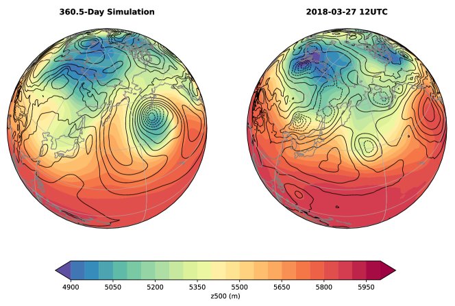
Figure 8: $Z_{500}$ (color fill: $50\text{\,}\mathrm{d}\mathrm{a}\mathrm{m}$ contour interval) and $Z_{1000}$ (black contours: $40\text{\,}\mathrm{m}$ interval) for a free-running 360.5-day simulation and the corresponding ERA5 reanalysis for 00 UTC on 27 March 2018. Dashed black lines indicate values of $Z_{1000}\leq$40\text{\,}\mathrm{m}$$ (corresponding to sea-level pressures less than roughly $1008\text{\,}\mathrm{h}\mathrm{P}\mathrm{a}$).

The roughly one-year lead time is well beyond the limits of atmospheric predictability, so there is no reason to expect a close match between simulation and reanalysis. The 360.5-day simulation time was chosen to display the simulated strong low-pressure center in the northeastern Pacific. The intensity of the system is typical for strong systems in our simulation, but about $40\text{\,}\mathrm{m}$ higher than the strongest systems periodically appearing in the ERA5 reanalysis. Lower-amplitude signals also appear in the $Z_{1000}$ field, which is somewhat less than $50\text{\,}\mathrm{m}$ too low in the tropics. In contrast to the simulation started on 1 July 2017 shown in Figure 7, the simulated $Z_{500}$ heights in the polar region in this simulation initialized on 1 April 2017 are not obviously lower than those in the ERA5 reanalysis. (We only conducted a pair of one-year rollout simulations to verify that they remained as stable as our previous Weyn et al. (2020) model.) On balance, the overall character of this late-March weather pattern is quite plausible.

In an ablation study, we investigated the effect of the top-of atmosphere solar forcing input on the 365-day rollout by training a model that did not receive solar forcing input. In that case, the model still generated a stable forecast over the entire rollout period, but did not produce the full annual cycle. Interestingly, that simulation did roughly approximate the transition from summer into a perpetual autumn.

A more quantitative assessment of any tendency of our model to distort the atmospheric state by damping or amplifying mid-latitude perturbations at different wavelengths is provided by the plots of the $Z_{500}$ power spectral density around $45\text{\,}{}^{\circ}\mathrm{N}$ in Figure 9. These spectra are averaged over 208 biweekly forecasts from the 2017-2018 test set; as such, the initial spectrum in black represents the average state of the atmosphere in the ERA5 reanalysis.

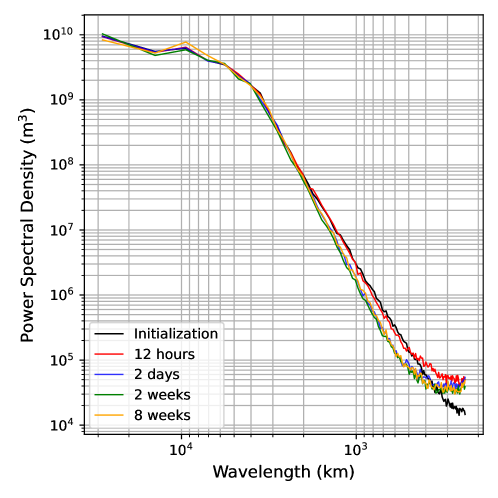
Figure 9: One dimensional power spectral density of the $Z_{500}$ field around the $45^{\circ}$ N latitude, averaged over 208 bi-weekly forecasts from 2017-2018 at: initialization (black), and at forecast lead times of $12\text{\,}\mathrm{h}$, $2\text{\,}\mathrm{d}$, 2, and 8 weeks.

Twelve hours (2 recursive steps) after initialization there is very little change in the spectra for wavelengths $\lambda$ longer than $500\text{\,}\mathrm{k}\mathrm{m}$ (roughly 5 grid intervals), but the power in the shorter waves is amplified. Over the next $36\text{\,}\mathrm{h}$, there is a gradual reduction in the amplitude at wavelengths $\lambda<$1800\text{\,}\mathrm{k}\mathrm{m}$$ to yield a spectrum that is modestly damped over the interval $380<\lambda<$1800\text{\,}\mathrm{k}\mathrm{m}$$ and amplified at the shortest wavelengths. Surprisingly, the spectral distribution at two days remains essentially unchanged through at least sub-seasonal forecast lead times of eight weeks, which is consistent with the impression obtained examining images such as those in Figure 8. There is no gradual amplification or loss of amplitude in the simulated atmospheric systems after the first two days.

5 Conclusion

We have presented an improved CNN-based DLWP-HPX model that stably forecasts atmospheric evolution over a full one-year cycle using a very limited set of prognostic variables. The number of actual degrees of freedom characterising predictable atmospheric states at forecast lead times beyond 3–5 days is not known, but is far less than the total number of prognostic variables carried at every grid cell in state-of-the-art NWP models. Here, we have demonstrated that realistic atmospheric simulations can be performed using just seven prognostic variables above each node on a HEALPix mesh with $110\text{\,}\mathrm{k}\mathrm{m}$ between the nodes.

The HEALPix mesh (Gorski et al., 2005) has been used in astronomy for almost two decades, but has previously seen very little use in atmospheric science. The mesh covers the sphere with a hierarchical grid of equal-area cells uniformly spaced along circles at constant latitudes. A particularly important advantage of the HEALPix mesh for weather forecasting with CNNs is that it is an “east to the right” mesh, i.e., east has the same orientation in every HEALPix cell. Weather systems tend to travel west-to-east in mid- and high-latitudes and east-to-west in the tropics. The kernel weights in our convolutional stencils can more economically learn this behavior than on our previous cubed sphere mesh in which the eastward orientation across the stencil varies with longitude, particularly on the polar faces. Although switching from a cube-sphere mesh with $64\times 64$ cells on each of the six faces to a HEALPix mesh with $32\times 32$ cells on each of the 12 faces reduces the total number of grid points covering the sphere by half, it improves the $Z_{500}$ RMSE error by almost one day at a 4-day forecast lead time (Figure 5).

Two other significant improvements to our model architecture were obtained by adding recursion via GRUs and by inverting the standard way channel depth is refined at deeper layers in the U-Net. In contrast to the original U-Net architecture Ronneberger et al. (2015), our channel depth halves instead of doubles as the spatial resolution is also halved in each successively deeper U-Net layer. This allows the model to devote more trainable parameters to describing the wide variety of fine-scale weather patterns while using comparatively fewer parameters to describe the simpler set of global weather patterns. Although this modification pushes the U-Net toward the basic ResNet architecture (He et al., 2016), we find the deeper U-Net layers continue to provide significant skill to the forecasts.

Additional modest improvements were implemented by switching to the GELU activation function and to $2\times 2$ transposed strided convolutions when up-sampling; by increasing the total number of trainable parameters from $2.7\text{\,}\mathrm{M}$ to $9.8\text{\,}\mathrm{M}$, adding the $Z_{250}$ field, increasing the resolution to HPX64, and increasing the time resolution to $3\text{\,}\mathrm{h}$ (which gives us a $6\text{\,}\mathrm{h}$ time step). The benefits of $3\text{\,}\mathrm{h}$ time resolution were only realized when the model included the GRUs. The $3\text{\,}\mathrm{h}$ time resolution gives a good forecast of the daily cycle of surface temperature, and the model also learns the difference in the range of that cycle between regions of tropical forest and desert without geo-specific input data.

Finally, we replaced the pairs of successive convolutions in Weyn et al. (2020) with modified ConvNeXt blocks. The switch to the ConvNeXt blocks was only advantageous at higher resolutions, where in addition to improving accuracy, it reduced the memory footprint.

At one-week forecast lead time, the resulting model is roughly 1 day behind the ECMWF IFS S2S forecast error in $Z_{500}$ RMSE and 1.5 days behind in ACC. These statistics are worse than those for Pangu-Weather (Bi et al., 2023) and GraphCast (Lam et al., 2022), both of which provide $Z_{500}$ RMSE and ACC forecasts at $0.25^{\circ}\times 0.25^{\circ}$ resolution that are superior to the ECMWF IFS high-resolution model averaged to the same $0.25^{\circ}\times 0.25^{\circ}$ grid. Despite having less accuracy in medium range forecasts, our model has some advantages relative to Pangu-Weather and GraphCast. In contrast to those models, ours can be recursively stepped forward for a full year while simulating realistic weather patterns. Our model also uses far less data to produce the forecast, employing just 7 spherical shells of data compared to 67 for Pangu-Weather, 227 for GraphCast, and 820 for the ECMWF IFS S2S forecast.

Deep learning models for weather forecasting are evolving rapidly, with important advancements using a wide variety of architectures. Our DLWP-HPX model provides an example of what can be achieved using a relatively parsimonius approach. As such, it may be particularly useful for scientific investigations where it is advantageous to work with a minimal set of unknown variables.

There are many avenues along which our DLPW-HPX model might be improved. One would be to adding additional prognostic fields while carefully examining the resulting performance. Another one would lie in refining the CNN architecture, where the choice of particular inductive biases may be crucial (Thuemmel et al., 2023). A related important aspect of improving the modelled processes might be to incorporate explicit physical constraints, yielding physics-informed differentiable artificial neural networks (Beucler et al., 2021; Shen et al., 2023). Other natural extensions of this work lie in examining the performance of the DLPW-HPX model in ensemble forecasts, which are crucial to sub-seasonal and seasonal prediction and to couple the atmospheric model with the ocean, thus moving toward a deep learning earth system model (Bauer et al., 2023).

Author Roles

Matthias implemented model, training and evaluation routines in PyTorch, as well as the HEALPix-related projection scripts under consideration of the healpy package, and drafted the manuscript together with Dale who supervised this project closely and who also sketched the model schematic in Figure 2. Nathaniel was involved in discussions about model evolution and code structures and generated Figure 6, Figure 7, and Figure 9. Raul was involved in model discussions and generated Figure 8. Thorsten helped with implementing the distributed PyTorch pipeline for multi-GPU training and with accelerating the process pipeline. Martin co-supervised this project and helped with proofreading and writing.

Appendix A Deep Learning on the HEALPix

A.1 Seamless Evolution of Location Invariant Kernels

The Hierarchical Equal Area isoLatitude Pixelization (HEALPix) is a partitioning of the sphere that has found wide application in astronomy since it was introduced by Gorski et al. (2005). It divides the sphere into 12 base faces that can be hierarchically subdivided into patches of equal size. A key property for training CNNs on this mesh is the isolatitudinal alignment, that is, patches are aligned along lines of latitude and each patch has the same orientation, which we describe as “east to the right” in Section 4.1.

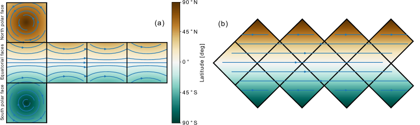
Figure 10: Lines of latitudes depicted as blue streamline arrows on the cubed sphere (a) and on the HEALPix (b). While the lines corresponding to constant eastward motion describe arcs of different radii on the cubed sphere mesh, the same motion translates to straight lines on the HEALPix mesh.

To contrast and emphasize the difficulty that CNN kernels are facing on the cubed sphere mesh, we plot the lines of constant latitude on the six faces of the cubed sphere and on the twelve faces of the HEALPix in Figure 10. Except for the equator, all lines of constant latitude are bent on the cubed sphere, imposing challenges for a limited set of convolution kernels that must evolve location invariant pattern detectors and functions. For example, on the cubed sphere, kernels need to learn a wider range of behaviors to propagate eastward motions at the top-left versus the top right corners of the cubed sphere faces.

On the other hand, lines of constant latitude map to straight lines on the HEALPix mesh. This facilitates the formulation of location-invariant convolutional kernels for the propagation of weather systems, which tend to migrate eastward outside the tropics.

A.2 Technical Implementation Details

Since deep learning libraries are optimized for image processing tasks, we consider each of the HEALPix’s 12 base faces as a regular two-dimensional tensor, i.e., we interpret the sphere as a composition of twelve images (cf. Figure 1 and Figure 11).

To simulate the spatial propagation of dynamics beyond individual faces, such that weather patterns can evolve globally on the sphere, we implement custom padding operations to concatenate the relevant information of all neighboring faces to each respective face of interest.

Figure 11 showcases our planet’s coastlines projected on the HEALPix faces in (a) and outlines the spatial organization of the twelve faces in (b). The arrangement of neighboring faces is exemplarily detailed for the northern (N) and southern (S) hemisphere, as well as for the equatorial faces (E). To simulate the neighborhood of, say, face E3, the face N2 must be concatenated to the left of E3, while face S3 is concatenated to the right. On the northern and southern hemispheres, neighboring faces are partially required to be rotated, as indicated in Figure 11 (c), (d), and (e).

A particular case occurs in the north and south corners of the tropical faces, where no natural neighbor exists—cf. Figure 1 and Figure 11 (f) for an illustration. To simulate the ninth neighbor of the respective corner, we interpolate the values from the according faces on the northern/southern hemisphere, by simply averaging the two corresponding values and writing the result in the simulated neighboring face. For example, to simulate the top left neighboring face of E3, we average the respective values from N2 and N3, as detailed by the straight red arrows in Figure 11 (g). Values that do not lie on the main diagonal of the simulated face are not required to be interpolated, but are copied from the adjacent faces instead, denoted by the curved red arrows in Figure 11 (g). The exemplary corner padding shows the case for the application of a $3\times 3$ kernel with dilation of 1 or 2. Note that a $5\times 5$ kernel could be applied in the same way. Importantly, the padding should not extend one neighboring face, which depends on the resolution of the HEALPix mesh and the configuration of the applied convolution (kernel size and dilation). Otherwise, a hierarchy of padding operations would be required to be implemented and considered.

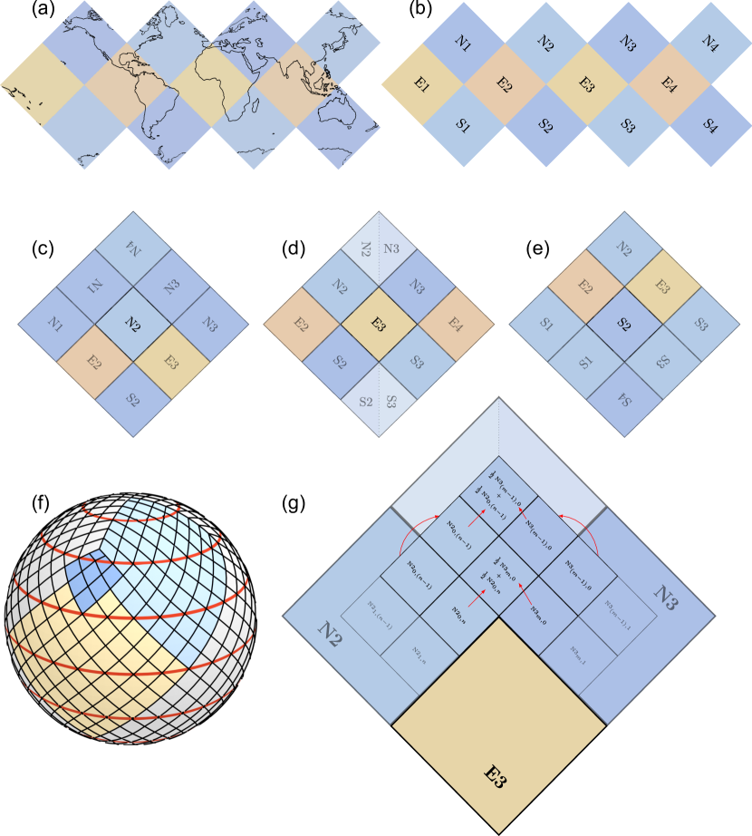
Figure 11: 2D HEALPix face arrangement and padding. (a) depicts the distribution of coastlines over the twelve HEALPix faces. (b) enumerates the twelve faces of the HEALPix with each four faces on the northern and southern hemisphere and around the equator. (c), (d), and (e): Exemplary alignment and rotations of neighboring faces before applying the padding operation on northern (c), equatorial (d), and southern faces (e). (f) emphasizes the special corner case, which is detailed in (g) to visualize the padding, where a ninth pixel is simulated by averaging the two respective values from the adjacent faces.

References

- Battaglia et al. (2018) Peter W Battaglia, Jessica B Hamrick, Victor Bapst, Alvaro Sanchez-Gonzalez, Vinicius Zambaldi, Mateusz Malinowski, Andrea Tacchetti, David Raposo, Adam Santoro, Ryan Faulkner, et al. Relational inductive biases, deep learning, and graph networks. arXiv preprint arXiv:1806.01261, 2018.
- Bauer et al. (2015) Peter Bauer, Alan Thorpe, and Gilbert Brunet. The quiet revolution of numerical weather prediction. Nature, 525(7567):47–55, 2015.
- Bauer et al. (2023) Peter Bauer, Peter Dueben, Matthew Chantry, Francisco Doblas-Reyes, Torsten Hoefler, Amy McGovern, and Bjorn Stevens. Deep learning and a changing economy in weather and climate prediction. Nature Reviews Earth & Environment, 4(8):507–509, 2023. ISSN 2662-138X. doi: 10.1038/s43017-023-00468-z. URL https://doi.org/10.1038/s43017-023-00468-z.
- Benjamin et al. (2019) Stanley G Benjamin, John M Brown, Gilbert Brunet, Peter Lynch, Kazuo Saito, and Thomas W Schlatter. 100 years of progress in forecasting and nwp applications. Meteorological Monographs, 59:13–1, 2019.
- Beucler et al. (2021) Tom Beucler, Michael Pritchard, Stephan Rasp, Jordan Ott, Pierre Baldi, and Pierre Gentine. Enforcing analytic constraints in neural networks emulating physical systems. Physical Review Letters, 126(9):098302, 2021.
- Bi et al. (2023) Kaifeng Bi, Lingxi Xie, Hengheng Zhang, Xin Chen, Xiaotao Gu, and Qi Tian. Accurate medium-range global weather forecasting with 3d neural networks. Nature, 2023. doi: doi.org/10.1038/s41586-023-06185-3.
- Bonev et al. (2023) Boris Bonev, Thorsten Kurth, Christian Hundt, Jaideep Pathak, Maximilian Baust, Karthik Kashinath, and Animas Anandkumar. Spherical fourier neural operators: Learning stable dynamics on the sphere. arXiv preprint arXiv:2306.03838, 2023.
- Charney et al. (1950) J. G. Charney, R. Fjörtoft, and J. Von Neumann. Numerical Integration of the Barotropic Vorticity Equation. Tellus A, 2(4), 1950.
- Chen et al. (2023) Kang Chen, Tao Han, Junchao Gong, Lei Bai, Fenghua Ling, Jing-Jia Luo, Xi Chen, Leiming Ma, Tianning Zhang, Rui Su, Yuanzheng Ci, Bin Li, Xiaokang Yang, and Wanli Ouyang. Fengwu: Pushing the skillful global medium-range weather forecast beyond 10 days lead. arXiv preprint arXiv:2304.02948, 2023.
- Cho et al. (2014) Kyunghyun Cho, B van Merrienboer, Caglar Gulcehre, F Bougares, H Schwenk, and Yoshua Bengio. Learning phrase representations using rnn encoder-decoder for statistical machine translation. In Conference on Empirical Methods in Natural Language Processing (EMNLP 2014), 2014.
- Dosovitskiy et al. (2020) Alexey Dosovitskiy, Lucas Beyer, Alexander Kolesnikov, Dirk Weissenborn, Xiaohua Zhai, Thomas Unterthiner, Mostafa Dehghani, Matthias Minderer, Georg Heigold, Sylvain Gelly, et al. An image is worth 16x16 words: Transformers for image recognition at scale. arXiv preprint arXiv:2010.11929, 2020.
- Dueben and Bauer (2018) Peter D. Dueben and Peter Bauer. Challenges and design choices for global weather and climate models based on machine learning. Geoscientific Model Development, 11(10):3999–4009, 2018.
- Gori et al. (2005) Marco Gori, Gabriele Monfardini, and Franco Scarselli. A new model for learning in graph domains. In Proceedings. 2005 IEEE International Joint Conference on Neural Networks, 2005., volume 2, pages 729–734. IEEE, 2005.
- Gorski et al. (2005) Krzysztof M Gorski, Eric Hivon, Anthony J Banday, Benjamin D Wandelt, Frode K Hansen, Mstvos Reinecke, and Matthia Bartelmann. Healpix: A framework for high-resolution discretization and fast analysis of data distributed on the sphere. The Astrophysical Journal, 622(2):759, 2005.
- Guibas et al. (2021) John Guibas, Morteza Mardani, Zongyi Li, Andrew Tao, Anima Anandkumar, and Bryan Catanzaro. Efficient token mixing for transformers via adaptive fourier neural operators. In International Conference on Learning Representations, 2021.
- He et al. (2016) Kaiming He, Xiangyu Zhang, Shaoqing Ren, and Jian Sun. Deep residual learning for image recognition. In Proceedings of the IEEE conference on computer vision and pattern recognition, pages 770–778, 2016.
- Hendrycks and Gimpel (2016) Dan Hendrycks and Kevin Gimpel. Gaussian error linear units (gelus). arXiv preprint arXiv:1606.08415, 2016.
- Hersbach et al. (2020) Hans Hersbach, Bill Bell, Paul Berrisford, Shoji Hirahara, András Horányi, Joaquín Muñoz-Sabater, Julien Nicolas, Carole Peubey, Raluca Radu, Dinand Schepers, et al. The era5 global reanalysis. Quarterly Journal of the Royal Meteorological Society, 146(730):1999–2049, 2020.
- Hochreiter and Schmidhuber (1997) Sepp Hochreiter and Jürgen Schmidhuber. Long short-term memory. Neural computation, 9(8):1735–1780, 1997.
- Hu et al. (2022) Yuan Hu, Lei Chen, Zhibin Wang, and Hao Li. Swinvrnn: A data-driven ensemble forecasting model via learned distribution perturbation. arXiv preprint arXiv:2205.13158, 2022.
- Huang et al. (2020) Huimin Huang, Lanfen Lin, Ruofeng Tong, Hongjie Hu, Qiaowei Zhang, Yutaro Iwamoto, Xianhua Han, Yen-Wei Chen, and Jian Wu. Unet 3+: A full-scale connected unet for medical image segmentation. In ICASSP 2020-2020 IEEE International Conference on Acoustics, Speech and Signal Processing (ICASSP), pages 1055–1059. IEEE, 2020.
- Keisler (2022) Ryan Keisler. Forecasting global weather with graph neural networks. arXiv preprint arXiv:2202.07575, 2022.
- Kingma and Ba (2014) Diederik P Kingma and Jimmy Ba. Adam: A method for stochastic optimization. arXiv preprint arXiv:1412.6980, 2014.
- Kipf and Welling (2016) Thomas N Kipf and Max Welling. Semi-supervised classification with graph convolutional networks. arXiv preprint arXiv:1609.02907, 2016.
- Krachmalnicoff and Tomasi (2019) Nicoletta Krachmalnicoff and Maurizio Tomasi. Convolutional neural networks on the healpix sphere: a pixel-based algorithm and its application to cmb data analysis. Astronomy & Astrophysics, 628:A129, 2019.
- Kurth et al. (2022) Thorsten Kurth, Shashank Subramanian, Peter Harrington, Jaideep Pathak, Morteza Mardani, David Hall, Andrea Miele, Karthik Kashinath, and Animashree Anandkumar. Fourcastnet: Accelerating global high-resolution weather forecasting using adaptive fourier neural operators. arXiv preprint arXiv:2208.05419, 2022.
- Lam et al. (2022) Remi Lam, Alvaro Sanchez-Gonzalez, Matthew Willson, Peter Wirnsberger, Meire Fortunato, Alexander Pritzel, Suman Ravuri, Timo Ewalds, Ferran Alet, Zach Eaton-Rosen, et al. Graphcast: Learning skillful medium-range global weather forecasting. arXiv preprint arXiv:2212.12794, 2022.
- Li et al. (2020) Zongyi Li, Nikola Kovachki, Kamyar Azizzadenesheli, Burigede Liu, Kaushik Bhattacharya, Andrew Stuart, and Anima Anandkumar. Fourier neural operator for parametric partial differential equations. arXiv preprint arXiv:2010.08895, 2020.
- Liu et al. (2021) Ze Liu, Yutong Lin, Yue Cao, Han Hu, Yixuan Wei, Zheng Zhang, Stephen Lin, and Baining Guo. Swin transformer: Hierarchical vision transformer using shifted windows. In Proceedings of the IEEE/CVF International Conference on Computer Vision, pages 10012–10022, 2021.
- Liu et al. (2022) Zhuang Liu, Hanzi Mao, Chao-Yuan Wu, Christoph Feichtenhofer, Trevor Darrell, and Saining Xie. A convnet for the 2020s. In Proceedings of the IEEE/CVF Conference on Computer Vision and Pattern Recognition, pages 11976–11986, 2022.
- Lopez-Gomez et al. (2022) Ignacio Lopez-Gomez, Amy McGovern, Shreya Agrawal, and Jason Hickey. Global extreme heat forecasting using neural weather models. arXiv preprint arXiv:2205.10972, 2022.
- Lorenz (1969) Edward N Lorenz. The predictability of a flow which possesses many scales of motion. Tellus, 21(3):289–307, 1969.
- Loshchilov and Hutter (2016) Ilya Loshchilov and Frank Hutter. Sgdr: Stochastic gradient descent with warm restarts. In International Conference on Learning Representations, 2016.
- Palmer (2019) Tim Palmer. The ecmwf ensemble prediction system: Looking back (more than) 25 years and projecting forward 25 years. Quarterly Journal of the Royal Meteorological Society, 145:12–24, 2019.
- Pathak et al. (2022) Jaideep Pathak, Shashank Subramanian, Peter Harrington, Sanjeev Raja, Ashesh Chattopadhyay, Morteza Mardani, Thorsten Kurth, David Hall, Zongyi Li, Kamyar Azizzadenesheli, et al. Fourcastnet: A global data-driven high-resolution weather model using adaptive fourier neural operators. arXiv preprint arXiv:2202.11214, 2022.
- Perraudin et al. (2019) Nathanaël Perraudin, Michaël Defferrard, Tomasz Kacprzak, and Raphael Sgier. Deepsphere: Efficient spherical convolutional neural network with healpix sampling for cosmological applications. Astronomy and Computing, 27:130–146, 2019.
- Pfaff et al. (2020) Tobias Pfaff, Meire Fortunato, Alvaro Sanchez-Gonzalez, and Peter W Battaglia. Learning mesh-based simulation with graph networks. arXiv preprint arXiv:2010.03409, 2020.
- Rasp and Thuerey (2021) Stephan Rasp and Nils Thuerey. Data-driven medium-range weather prediction with a resnet pretrained on climate simulations: A new model for weatherbench. Journal of Advances in Modeling Earth Systems, 13(2):e2020MS002405, 2021.
- Ronneberger et al. (2015) Olaf Ronneberger, Philipp Fischer, and Thomas Brox. U-net: Convolutional networks for biomedical image segmentation. In International Conference on Medical image computing and computer-assisted intervention, pages 234–241. Springer, 2015.
- Scarselli et al. (2008) Franco Scarselli, Marco Gori, Ah Chung Tsoi, Markus Hagenbuchner, and Gabriele Monfardini. The graph neural network model. IEEE transactions on neural networks, 20(1):61–80, 2008.
- Scher and Messori (2018) Sebastian Scher and Gabriele Messori. Predicting weather forecast uncertainty with machine learning. Quarterly Journal of the Royal Meteorological Society, 144(717):2830–2841, 2018.
- Scher and Messori (2019) Sebastian Scher and Gabriele Messori. Weather and climate forecasting with neural networks: using GCMs with different complexity as study-ground. Geoscientific Model Development, 12:2797–2809, 2019.
- Shen et al. (2023) Chaopeng Shen, Alison P. Appling, Pierre Gentine, Toshiyuki Bandai, Hoshin Gupta, Alexandre Tartakovsky, Marco Baity-Jesi, Fabrizio Fenicia, Daniel Kifer, Li Li, Xiaofeng Liu, Wei Ren, Yi Zheng, Ciaran J. Harman, Martyn Clark, Matthew Farthing, Dapeng Feng, Praveen Kumar, Doaa Aboelyazeed, Farshid Rahmani, Yalan Song, Hylke E. Beck, Tadd Bindas, Dipankar Dwivedi, Kuai Fang, Marvin Höge, Chris Rackauckas, Binayak Mohanty, Tirthankar Roy, Chonggang Xu, and Kathryn Lawson. Differentiable modelling to unify machine learning and physical models for geosciences. Nature Reviews Earth & Environment, 4(8):552–567, 2023. ISSN 2662-138X. doi: 10.1038/s43017-023-00450-9. URL https://doi.org/10.1038/s43017-023-00450-9.
- Thuemmel et al. (2023) Jannik Thuemmel, Matthias Karlbauer, Sebastian Otte, Christiane Zarfl, Georg Martius, Nicole Ludwig, Thomas Scholten, Ulrich Friedrich, Volker Wulfmeyer, Bedartha Goswami, et al. Inductive biases in deep learning models for weather prediction. arXiv preprint arXiv:2304.04664, 2023.
- Tobler (1970) Waldo R Tobler. A computer movie simulating urban growth in the detroit region. Economic geography, 46(sup1):234–240, 1970.
- Vaswani et al. (2017) Ashish Vaswani, Noam Shazeer, Niki Parmar, Jakob Uszkoreit, Llion Jones, Aidan N Gomez, Łukasz Kaiser, and Illia Polosukhin. Attention is all you need. Advances in neural information processing systems, 30, 2017.
- Vitart (2004) Frédéric Vitart. Monthly forecasting at ECMWF. Monthly Weather Review, 132:2761–2779, 2004. doi: 10.1175/MWR2826.1.
- Weigel et al. (2008) Andreas P. Weigel, Daniel Baggenstos, Mark A. Liniger, Frédéric Vitart, and Christof Appenzeller. Probabilistic Verification of Monthly Temperature Forecasts. Monthly Weather Review, 136:5162–5182, 2008. doi: 10.1175/2008MWR2551.1.
- Weyn et al. (2019) Jonathan A Weyn, Dale R Durran, and Rich Caruana. Can machines learn to predict weather? using deep learning to predict gridded 500-hpa geopotential height from historical weather data. Journal of Advances in Modeling Earth Systems, 11(8):2680–2693, 2019.
- Weyn et al. (2020) Jonathan A Weyn, Dale R Durran, and Rich Caruana. Improving data-driven global weather prediction using deep convolutional neural networks on a cubed sphere. Journal of Advances in Modeling Earth Systems, 12(9):e2020MS002109, 2020.
- Weyn et al. (2021) Jonathan A Weyn, Dale R Durran, Rich Caruana, and Nathaniel Cresswell-Clay. Sub-seasonal forecasting with a large ensemble of deep-learning weather prediction models. Journal of Advances in Modeling Earth Systems, 13(7):e2021MS002502, 2021.
- Zhou et al. (2018) Zongwei Zhou, Md Mahfuzur Rahman Siddiquee, Nima Tajbakhsh, and Jianming Liang. Unet++: A nested u-net architecture for medical image segmentation. In Deep learning in medical image analysis and multimodal learning for clinical decision support, pages 3–11. Springer, 2018.