The Scale of Homogeneity in the $R_{\rm h}=ct$ Universe

Abstract

Studies of the Universe’s transition to smoothness in the context of $\Lambda$CDM have all pointed to a transition radius no larger than $\sim 300$ Mpc. These are based on a broad array of tracers for the matter power spectrum, including galaxies, clusters, quasars, the Ly-$\alpha$ forest and anisotropies in the cosmic microwave background. It is therefore surprising, if not anomalous, to find many structures extending out over scales as large as $\sim 2$ Gpc, roughly an order of magnitude greater than expected. Such a disparity suggests that new physics may be contributing to the formation of large-scale structure, warranting a consideration of the alternative FLRW cosmology known as the $R_{\rm h}=ct$ universe. This model has successfully eliminated many other problems in $\Lambda$CDM. In this paper, we calculate the fractal (or Hausdorff) dimension in this cosmology as a function of distance, showing a transition to smoothness at $\sim 2.2$ Gpc, fully accommodating all of the giant structures seen thus far. This outcome adds further observational support for $R_{\rm h}=ct$ over the standard model.

1 Introduction

The standard model of cosmology ($\Lambda$CDM; Ostriker & Steinhardt 1995) is based on the Friedmann-Lemaître-Robertson-Walker (FLRW) spacetime, whose metric coefficients reflect the symmetries assumed by the cosmological principle, i.e., isotropy and homogeneity (Melia, 2020), at least on large scales. Of the two, isotropy is easier to measure, since the observations can be carried out from a single vantage point, using the cosmic microwave background (CMB; Schwarz et al. 2016; Planck Collaboration et al. 2016), galaxy and radio source counts (Rameez et al., 2018), weak lensing convergence (Marques et al., 2018), and Type Ia supernovae (Andrade et al., 2018).

Homogeneity is measured less reliably because we can only probe structure down our past lightcone, not directly on a time-constant hypersurface (Clarkson et al., 2012). One must interpret these measurements in the context of how well the model predictions are confirmed by the observed structure evolution within the past lightcone. Observational tests of homogeneity have been carried out by several workers, using various tracers of the matter distribution, including galaxies, clusters of galaxies, the Ly-$\alpha$ forest and quasars (Hogg et al., 2005; Scrimgeour et al., 2012; Alonso et al., 2015; Laurent et al., 2016; Ntelis et al., 2017; Gonçalves et al., 2018; Secrest et al., 2021; Camacho-Quevedo & Gaztañaga, 2022). These studies typically employ the so-called fractal (or correlation) dimension (see Eq. 10 below) to characterize the spatial scale at which homogeneity is attained.

In the majority of cases, the transition is quoted at $\sim 100-200\;{\rm Mpc}/h$, where $h\equiv H_{0}/100$ km s^-1 Mpc^-1 is the scaled Hubble parameter. Throughout this paper, we shall conveniently adopt the Planck value optimized for $\Lambda$CDM, i.e., $h=0.6732$ (Planck Collaboration et al., 2016). Some studies possibly stretch the range to $\sim 260\;{\rm Mpc}/h$ (Yadav et al., 2010). Very importantly, however, no study has yet shown a termination of the clustering on scales larger than $\sim 300$ Mpc.

So it comes as a surprise to learn that cosmic structures can form bigger—even much bigger—than this limit. A sample discovered thus far is shown in Table 1 below. This includes the Giant GRB Ring, traced by 9 gamma-ray bursts (GRBs) at $z\sim 0.82$, with a diameter of $\sim 1720$ Mpc (Balázs et al., 2015). With a probability of $\sim 2\times 10^{-6}$ of this being merely the result of random GRB count rate fluctuations, the structure appears to be seen as a projection of a shell on the plane of the sky. The largest structure seen thus far appears to be the Hercules-Corona Borealis Great Wall (HCB Great Wall), also identified via a large GRB cluster at $z\sim 2$ with a size of $2000-3000$ Mpc (Horváth et al., 2014). Its angular size remarkably covers one-eighth of the sky. Other large structures have been identified via quasar associations, e.g., the Huge-LQG (Huge-Large Quasar Group) centered at $z=1.27$ with a size of $1240$ Mpc (Clowes et al., 2012; Hutsemékers et al., 2014), and in galaxy surveys, including the Sloan Great Wall of galaxies at $z\sim 0.073$ with a length of $450$ Mpc (Gott et al., 2005).

Table 1: Sample of very large structures identified thus far.

Name	Mean redshift	Proper Size	Reference
		(Mpc)
HCD Great Wall	$\sim 2$	2000-3000	Horváth et al. (2014); Christian (2020)
Giant GRB Ring	$0.82$	1720	Balázs et al. (2015)
Correlated LQG Orientations	$1.0-1.8$	1600	Friday et al. (2022)
U1.27, Huge-LQG	$1.27$	1240	Clowes et al. (2012); Hutsemékers et al. (2014)
Giant Arc	$\sim 0.8$	1000	Lopez et al. (2022)
Coherent Quasar Polarizations	$1-2$	1000	Hutsemékers et al. (2005)
U1.11	$1.11$	780	Clowes et al. (2012)
U1.28, CCLQG	$1.28$	630	Clowes et al. (2012)
Sloan Great Wall	$0.073$	450	Gott et al. (2005)
South Pole Wall	$0.04$	420	Pomarède et al. (2020)
Blazar LSS	$\sim 0.35$	350	Marchã & Browne (2021)
Local Void	$<0.07$	300	Whitbourn & Shanks (2016)

But there are other observational indications that the generic assumption of smoothness on scales exceeding $\sim 200$ Mpc in the standard model is not well supported by the data. For example, in their statistical analysis of the visible matter distribution, Coleman & Pietronero (1992) concluded that it is fractal and multifractal on such scales, without any evidence of termination, i.e., homogenization. Subsequent work (Sylos Labini et al., 1998, 2009) confirmed that galaxy structures are irregular and self-similar, consistent with fractal correlations up to scales exceeding $\sim 1$ Gpc. The implication is that the distribution of matter is not analytic and cannot be described in terms of a simple average density. These inhomogeneities therefore appear to challenge our conventional view of cosmology (Sylos Labini, 2011). It has even been suggested that an otherwise smooth metric, such as the Lemaître-Tolman-Bondi universe, that is able to describe, on average, a fractal distribution of matter, may explain cosmic acceleration as a purely fractal phenomenon (Cosmai et al., 2019). As we shall see in this paper, however, the transition to smoothness is heavily model dependent so, while this type of statistical analysis does not comport very well with the small transition to smoothness scale predicted by $\Lambda$CDM, it would be fully consistent with an alternative model that predicts a much larger scale of homogeneity, well beyond the fractal domain.

The discovery of super large structures comes with several important caveats, that we shall discuss in greater detail below. First, we are actually dealing with two overlapping issues: the average transition to smoothness versus statistical fluctuations forming anomalously large structures. These are not necessarily incompatible with each other (Nadathur, 2013). Second, it is not certain that we have detected the largest structures yet. In their implementation of the Zipf-Mandelbrot law to the size distribution of superclusters of galaxies, De Marzo et al. (2021) conclude that none of the currently available catalogs are sufficiently large for us to have seen a truncation in their extent. Deeper redshift surveys may yet uncover even larger structures than the greatest already observed.

No matter how one interprets these results, however, the discovery of structures an order of magnitude larger than the transition to smoothness begs for an explanation. In this paper, we examine this issue in the context of the alternative FLRW cosmology known as the $R_{\rm h}=ct$ universe (Melia, 2007; Melia & Shevchuk, 2012; Melia, 2020). This model has been discussed extensively in both the primary and secondary literature, so we won’t dwell on its foundational and observational details in this paper, except to highlight the fact that, viewed as an advanced version of $\Lambda$CDM, it actually solves many of the current standard model’s conflicts and tensions (Melia, 2022). The most recent comparative study, based on the surprising detection by JWST of large well formed galaxies at much higher redshifts than can be accommodated by $\Lambda$CDM (Pontoppidan et al., 2022; Finkelstein et al., 2022; Treu et al., 2022; Robertson et al., 2022), has shown that the timeline in $R_{\rm h}=ct$ is much more compatible with the implied formation of structure in the early Universe (Melia, 2023).

The improvements introduced by this ‘advanced’ version of the standard model are therefore not merely cosmetic. It solves most, if not all, of $\Lambda$CDM’s long-standing problems. The consistency between the formation of structure in $R_{\rm h}=ct$ and the most recent observations by JWST therefore suggests that the creation of the anomalously large features listed in Table 1 may be more compatible with this alternative FLRW cosmology.

Given that the creation of structure is tightly related to the physics of star, galaxy, and cluster formation, the anomalies we explore in this paper, specifically how $\sim 2$ Gpc structures could possibly have formed in an FLRW Universe, are of significant importance to ongoing and future surveys of the Universe at intermediate and high redshifts.

2 Scale of Homogeneity

A technique commonly used to determine the spatial distance at which the large-scale structure transitions to homogeneity is based on multifractal analysis, in which the fractal dimension, $D_{2}$, of the underlying point distribution approaches the ambient dimension, $D=3$, of the space where the points lie (Bagla et al., 2008; Yadav et al., 2010). In reality, $D_{2}$ never quite reaches 3, so an alternative, less definitive, criterion needs to be defined. An example of this was the suggestion by Yadav et al. (2010) to use the distance at which the deviation, $(\Delta D_{2})_{\rm clus}$, of the fractal dimension due to clustering becomes smaller than its statistical dispersion.

The definition of a ‘homogeneity scale’ tends to be somewhat arbitrary because the approach to homogeneity is gradual, not abrupt. The proposal by Yadav et al. (2010) has been questioned because in deriving the dispersion they ignored the contribution to variance from the survey geometry and selection function. The dispersion calculated from a real survey is therefore not easily interpreted using this definition, certainly not when comparing different samples derived with inconsistent selection criteria. A more commonly used definition of the ‘homogeneity scale’ today is the distance, $r_{\mathcal{H}}$, at which the deviation of the fractal dimension due to clustering drops to $1\%$ of $D$ (Scrimgeour et al., 2012).

Detailed information on clustering within the distribution is inferred from a correlation integral,

$$C_{2}\equiv{1\over NM}\sum_{i=1}^{M}n_{i}(r)\;,$$ (1)

where $N$ is the number of points in the distribution, $M$ is the number of spheres of radius $r$ (much smaller than the overall size of the space), and $n(r)$ is the number of points within a distance $r$ from the $i^{\rm th}$ point:

$$n_{i}(r)\equiv\sum_{j=1}^{N}\Theta(r-|s_{i}-s_{j}|)\;.$$ (2)

Here, $\Theta$ is the Heaviside function, and $|s_{i}-s_{j}|$ is the distance between each pair of points $(i,j)$.

Depending on how the points are clustered (if at all), the fractal dimension changes with $r$—and presumably approaches that of the space ($D$) asymptotically. The Minkowski-Bouligand dimension is defined as (Yadav et al., 2010)

$$D_{2}(r)\equiv{d\,\log C_{2}(r)\over d\,\log r}\;.$$ (3)

If the distribution is homogeneous, then clearly $C_{2}(r)\propto r^{3}$ and $D_{2}(r)=3$, for a space with dimension $D=3$.

The geometrical sampling of a given survey is not perfect, however, so a scaled correlation integral was introduced (Scrimgeour et al., 2012), which is just $C_{2}(r)$ normalized by the same quantity in a random homogeneous distribution (including selection effects, if present):

$${\mathcal{N}}\equiv{C_{2}(r)\over\bar{C}_{2}(r)}\;,$$ (4)

where

$$\bar{C}_{2}(r)\equiv{4\pi\over 3}r^{3}\bar{n}\;,$$ (5)

in terms of the average number density, $\bar{n}$.

Equation (1) may be written in terms of the two-point correlation function, $\xi(r)$, starting with the differential (Ntelis et al., 2017)

$$dC_{2}(r)=\bar{n}\left[1+\xi(r)\right]dV\;,$$ (6)

where $dV$ is the differential volume around a given particle. The integrated correlation integral is then simply

$$C_{2}(r)=4\pi\bar{n}\int_{0}^{r}\left[1+\xi(u)\right]u^{2}\,du\;,$$ (7)

under the assumption of isotropy, for which $\xi({\bf r})=\xi(r)$. It is straightforward to see that Equation (4) then becomes

$${\mathcal{N}}(r)=1+{3\over r^{3}}\int_{0}^{r}\xi(u)u^{2}\,du\;.$$ (8)

It is not difficult to see from Equations (3) and (4) that the fractal correlation dimension may also be written as

$$D_{2}(r)={d\,\log{\mathcal{N}}\over d\,\log r}+D\;.$$ (9)

We may thus define the homogeneity index, ${\mathcal{H}}$, a fractal or Hausdorff dimension, which in this context represents the deviation $(\Delta D_{2})_{\rm clus}$, as

$${\mathcal{H}}\equiv{d\,\log{\mathcal{N}}\over d\,\log r}.$$ (10)

Complete homogeneity is thus reached when ${\mathcal{H}}=0$ (or $D_{2}=D$).

If we now define the volume-averaged two-point correlation function

$$\bar{\xi}(r)\equiv{3\over r^{3}}\int_{0}^{r}\xi(u)u^{2}\,du\;,$$ (11)

we see that

$${\mathcal{N}}=1+\bar{\xi}\;,$$ (12)

and therefore

$${\mathcal{H}}={D\over 1+\bar{\xi}}\left[\xi-\bar{\xi}\right]\;.$$ (13)

Note that this expression is not restricted by any assumption concerning the magnitude of $\xi$ or $\bar{\xi}$. For the rest of this paper, we shall follow current convention and assume that homogeneity is reached when ${\mathcal{H}}$ is $<1\%$ of $D$, i.e., for $|{\mathcal{H}}|<0.03$ in 3-dimensional space (Scrimgeour et al., 2012; Laurent et al., 2016; Ntelis et al., 2017; Gonçalves et al., 2018).

3 The two-point correlation function

The two-point correlation function may be expressed in terms of its Fourier transform, the power spectrum, $P(k)$, according to

$$\xi(s)={1\over(2\pi)^{3/2}}\int P(k)e^{-i{\bf k}\cdot{\bf s}}d^{3}k\;.$$ (14)

For an isotropic distribution, one may integrate this expression over angles and obtain the one-dimensional integral

$$\xi(s)={1\over 2\pi^{2}}\int_{0}^{\infty}k^{2}\,dk\,P(k)j_{0}(ks)\;,$$ (15)

where

$$j_{0}(x)={\sin(x)\over x}$$ (16)

is a spherical Bessel function.

As discussed above, the matter distribution may be measured using several different kinds of tracers, including galaxies, quasars, clusters of galaxies, fluctuations in the CMB and the Ly-$\alpha$ forest. Previous work has shown that all of these measurements tend to yield similar values of the transition radius, typically in the range $\sim 100-200\;{\rm Mpc}/h$. A principal concern of our comparative analysis is the proper recalibration of these data for each individual cosmology, given that densities and distances vary from one model to the next. Since we are primarily interested in finding variations from $\sim 300$ Mpc to $\sim 2000$ Mpc, rather than incremental differences from one type of object to the next within the same background cosmology, we shall conveniently choose a set of data for which the recalibration is quite straightforward, i.e., we shall simply use the fluctuations in the CMB and the Ly-$\alpha$ forest, more fully described in Yennapureddy & Melia (2021).

These data are compared to the theoretical predictions in Figures (1) and (2) for $\Lambda$CDM and $R_{\rm h}=ct$, respectively, calculated from the assumed primordial power spectrum and the transfer functions in these models. These two figures look quite different from each other because the data are not model-independent. The CMB measurements in these diagrams are shown as blue, orange and black circular dots. These are calculated from the CMB observations (Planck Collaboration et al., 2016) using the approach of Tegmark & Zaldarriaga (2002).

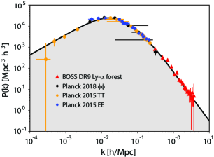
Figure 1: The matter power spectrum based on observations of the CMB (orange, blue and black dots), and the Ly-$\alpha$ survey (red triangles), compared with the power spectrum predicted by $\Lambda$CDM (solid black curve). Here, $h$ is the parameter $H_{0}/(100\;{\rm km}\;{\rm s}^{-1}\;{\rm Mpc}^{-1})$. Throughout this paper, we assume the value $h=0.6732$, consistent with the latest Planck measurements (Planck Collaboration et al. 2016). (Adapted from Yennapureddy and Melia 2021)

The Ly-$\alpha$ forest (shown as red triangles in Figs. 1 and 2) is due to the absorption along the line-of-sight of high-redshift quasar spectra. The fluctuations result from the inhomogeneous neutral hydrogen within the photo-ionized intergalactic medium. Since the underlying mass density is related to the optical depth of the Ly-$\alpha$ absorption line, the Ly-$\alpha$ forest is a proxy for the matter power spectrum. The amplitude of the fluctuations is itself model-dependent, however, so the Ly-$\alpha$ data must also be recalibrated for each individual cosmology. A caveat here is that the hydro simulations used to translate the absorption profile into the matter fluctuations are based on the behavior of dark matter only, and may not have included all of the relevant physics. Uncertainties in the reionization history, the ionizing background and its fluctuations may therefore be propagating in unreliable ways through the reconstruction of $P(k)$. As such, the Ly-$\alpha$ data may not be as reliable as the other points shown in this figure (see Yennapureddy & Melia 2021 for all the details).

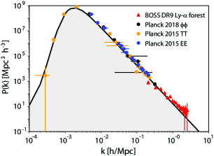
Figure 2: Same as Fig. 1, except here the data are calibrated for (and compared with) the $R_{\rm h}=ct$ cosmology (solid black curve). As before, $h=0.6732$ is the parameter $H_{0}/(100\;{\rm km}\;{\rm s}^{-1}\;{\rm Mpc}^{-1})$, consistent with the latest Planck measurements (Planck Collaboration et al. 2016). (Adapted from Yennapureddy and Melia 2021)

Insofar as this paper is concerned, the most important conclusion we can draw from Figures 1 and 2 is the remarkable consistency between the predicted power spectrum in both models and all of the available data. We can see the broad agreement between theory and the observations quantitatively via the reduced $\chi^{2}$ of the fits. The theoretical curves shown here are calculated simply using the Planck parameters without any optimization. For $\Lambda$CDM, one finds $\chi^{2}_{\rm dof}\approx 1.31$; the corresponding value for $R_{\rm h}=ct$ is $\chi^{2}_{\rm dof}\approx 1.3$. The fits could be improved slightly with additional optimization, but that is not really the focus of this paper. Demonstrating this consistency is the main reason for showing both the theoretical curves and the data, because we are thus confident that using the theoretically calculated curve for $P(k)$ provides an accurate assessment of the two-point correlation function predicted in both $\Lambda$CDM and $R_{\rm h}=ct$ via Equation (15). In other words, our estimation of the transition radius is fully based on the ‘observed’ two-point correlation function in both models. It is not merely an untested theoretical prediction.

The two-point correlation function derived from Figure (1) for $\Lambda$CDM is well known, so we don’t need to reproduce it here. The corresponding result for $R_{\rm h}=ct$, derived from Figure (2), is shown in Figure (3a).

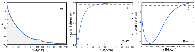
Figure 3: (a) The two-point correlation function, $\xi(r)$, as a function of $r/h$, calculated in the $R_{\rm h}=ct$ universe from the matter power spectrum in Fig. 2. (b) Homogeneity index estimated from the matter power spectrum in Fig. 1, calibrated for the concordance $\Lambda$CDM model. Using the nominal definition of a threshold to smoothness when $|\mathcal{H}|$ is less than $1\%$ of the space dimension, $D=3$, we infer a comoving transition distance $r_{\mathcal{H}}^{\Lambda{\rm CDM}}\sim 80\;{\rm Mpc}/h$. (c) Homogeneity index estimated from the matter power spectrum in Fig. 2, calibrated for the $R_{\rm h}=ct$ universe. Using the smoothness transition at $|\mathcal{H}|$ equal to $1\%$ of the space dimension, $D=3$, we infer a comoving transition distance $r_{\mathcal{H}}^{R_{\rm h}=ct}\sim 2,290\;{\rm Mpc}/h$.

4 Scale of homogeneity in $R_{\rm h}=ct$

As a sanity check, let us first calculate the fractal (or Hausdorff) dimension for $\Lambda$CDM to demonstrate consistency with previous work. ${\mathcal{H}}(r)$ in this model is shown as a function of $r$ in Figure (3b). The conventional definition of a threshold to smoothness, i.e., $|{\mathcal{H}}|<0.03$, implies that the $\Lambda$CDM universe becomes homogeneous on scales larger than $\sim 80\;{\rm Mpc}/h$. This outcome is entirely consistent with other estimations based on the use of various tracers of the matter distribution. ${\mathcal{H}}(r)$ is effectively zero by the time $r$ gets to several hundred Mpc and above. This is the reason, of course, why the much larger structures listed in Table 1 appear to be anomalous in this model.

The corresponding fractal (or Hausdorff) dimension for the $R_{\rm h}=ct$ universe is shown as a function of $r$ in Figure (3c). Evidently, homogeneity in this model is reached on scales greater than about $2200\;{\rm Mpc}/h$, about an order of magnitude larger than its counterpart in the standard model. The principal reason for this difference is not difficult to understand. Its root cause is the same physics responsible for the timeline in $R_{\rm h}=ct$ allowing large galaxies to form by redshift $\sim 17$, as recently discovered by JWST. Though the age of the Universe is about the same today in both models, roughly equal to $1/H_{0}$, the time versus redshift relation was stretched out by about a factor 2 at $z\gtrsim 6$ in $R_{\rm h}=ct$. The linear growth of structure therefore extended for longer in this model compared to $\Lambda$CDM, allowing structure to grow to much larger scales. Not only did large, well-formed galaxies appear at higher redshifts in $R_{\rm h}=ct$, but the deviation from homogeneity due to clustering was also enhanced by about an order of magnitude in scale.

5 Discussion

At face value, the outcome with $R_{\rm h}=ct$ would appear to be much more consistent with the existence of very large structures (Table 1) than the corresponding case in $\Lambda$CDM. It is also worth mentioning that observational evidence of anomalously large structures is independently provided by the measurement of the impact of large dark matter fluctuations on the CMB via the integrated Sachs-Wolfe effect (ISW) (Flender et al., 2013). The magnitude of the observed signal is more than $3\sigma$ larger than the theoretical $\Lambda$CDM expectation, indicating that dark matter inhomogeneities on scales beyond $\sim 100\;{\rm Mpc}/h$ are larger than expected.

As noted earlier, however, there are several caveats to this simple-minded comparison. We may not have seen the largest structure yet. Though in principle all such features discovered thus far are consistent with the clustering deviation from homogeneity in $R_{\rm h}=ct$, we would need to revisit this interpretation should future, deeper surveys uncover yet larger structures. Then the question of whether FLRW is truly the correct metric to use in cosmology would become a pressing issue.

The more serious caveat, though, is whether the discovery of very large structures should be viewed as a violation of the averaged transition to smoothness on smaller scales. At a very minimum, we should ask whether the linear growth phase had sufficient time to produce such large clustering with $\Lambda$CDM as the background cosmology. It certainly did in the case of $R_{\rm h}=ct$. But what about the standard model?

The answer may depend on the actual scale of the large structures. For example, the Sloan Great Wall has been known for almost twenty years (Gott et al., 2005). This filamentary structure identified in the Sloan Digital Sky Survey galaxy distribution extends over $\sim 450$ Mpc and has been viewed as an extremely unlikely occurrence in $\Lambda$CDM (Sheth & Diaferio, 2011). Nevertheless, some $N$-body simulations show that structures as large as this do emerge in a $\Lambda$CDM background (Park et al., 2012). Still, the probability for forming even larger structures, such as the Giant Arc (Lopez et al., 2022) and beyond, drops precipitously as the size increases.

An argument is sometimes made that structures such as the Huge-LQG (Clowes et al., 2012) are so physically large that they could not represent gravitationally bound systems in standard cosmology—this is another way of saying that there would not have been sufficient time for them to grow within the standard timeline. And given that clustering algorithms may find such extended features even in pure Poisson noise then means that, though they may be seen in the data, they do not actually represent real physical correlations (Nadathur, 2013). This is certainly true, but it ignores the possibility that the background cosmology may simply not be $\Lambda$CDM. As noted earlier, the timeline beyond $z\sim 6$ is stretched by about a factor $2$ in $R_{\rm h}=ct$ and, as we can see in Figures (2) and (3c), the linear growth phase in this model could adequately permit such large structures to grow gravitationally by the redshift at which we see them today.

The stark contrast seen between $\Lambda$CDM and $R_{\rm h}=ct$ in Figures (3b) and (3c) will likely also impact the expected appearance of our past cosmological lightcone (Carfora & Familiari, 2021, 2022). The issue here is how this lightcone is modified as a function of proper distance from the observer, given that the assumption of homogeneity in the FLRW metric breaks down on small spatial scales. A formal definition of the differences one may expect bears on several key observational signatures, including the angular diameter distance and lensing distortions.

A chief difficulty with the interpretation of the FLRW spacetime geometry arises when past lightcone data are gathered in our cosmological neighborhood, where the matter distribution becomes highly anisotropic with a high density contrast. On scales where this lack of smoothness becomes predominant, the Einstein evolution of the FLRW spacetime is, at best, an approximation, certainly not an accurate representation of the actual dynamics. Carfora & Familiari (2022) characterize this in terms of the distance-dependent level of tension one ought to observe between the model predictions and the observations, such that different models with different scales at which the transition to homogeneity is expected should experience measurably different levels of discordance arising from the simplifying assumption of homogeneity everywhere. Thus, in addition to the expected variation of the smoothness transition scale from one model to the next, it is reasonable to anticipate a distance-dependent variation of the tension with future high precision measurements that extends to larger scales when the real Universe is more anisotropic than the model predicts.

6 Conclusion

More and more we are seeing growing tension between the formation of structure predicted by the standard model and the actual observations. This is manifested in the surprisingly rapid formation of supermassive black holes, the too early appearance of galaxies, and the incorrect mass distribution of dark matter halos at $z\gtrsim 4$ (see Melia 2022, and references cited therein). The disparity between theory and the data has reached a high point with JWST’s recent detection of large, well-formed galaxies at $z\sim 17$ (Pontoppidan et al., 2022; Finkelstein et al., 2022; Treu et al., 2022; Robertson et al., 2022).

In all these cases, the timeline expected within the $R_{\rm h}=ct$ cosmology not only mitigates the tension, but appears to be fully consistent with the evolution of all these systems (Melia, 2014; Melia & McClintock, 2015; Yennapureddy & Melia, 2018). As an advanced version of $\Lambda$CDM, it is therefore sufficiently well supported by the data for us to continue its development and testing. In this paper, we have taken the next step by examining the impact of its extended timeline on the formation of the largest structures. We have found that the transition to homogeneity in this cosmology is expected to occur at a spatial scale $\sim 2200\;{\rm Mpc}/h$, comfortably beyond all of the large features discovered in the cosmos thus far.

There are some indications, however, that none of the existing catalogs are yet large enough for us to have seen the largest structure (De Marzo et al., 2021). If future, deeper surveys find correlations in the matter distribution well beyond $\sim 2200\;{\rm Mpc}/h$, we may have to seriously rethink the suitability of the FLRW metric for the description of our cosmic spacetime.

DATA AVAILABILITY STATEMENT

No new data were generated or analyzed in support of this research.

References

- Alonso et al. (2015) Alonso D., Salvador A. I., Sánchez F. J., Bilicki M., García-Bellido J., Sánchez E., 2015, MNRAS , 449, 670
- Andrade et al. (2018) Andrade U., Bengaly C. A. P., Santos B., Alcaniz J. S., 2018, ApJ, 865, 119
- Bagla et al. (2008) Bagla J. S., Yadav J., Seshadri T. R., 2008, MNRAS , 390, 829
- Balázs et al. (2015) Balázs L. G., Bagoly Z., Hakkila J. E., Horváth I., Kóbori J., Rácz I. I., Tóth L. V., 2015, MNRAS , 452, 2236
- Camacho-Quevedo & Gaztañaga (2022) Camacho-Quevedo B., Gaztañaga E., 2022, JCAP, 2022, 044
- Carfora & Familiari (2021) Carfora M., Familiari F., 2021, Letters in Mathematical Physics, 111, 53
- Carfora & Familiari (2022) Carfora M., Familiari F., 2022, Universe, 9, 25
- Christian (2020) Christian S., 2020, MNRAS , 495, 4291
- Clarkson et al. (2012) Clarkson C., Clifton T., Coley A., Sung R., 2012, PRD , 85, 043506
- Clowes et al. (2012) Clowes R. G., Campusano L. E., Graham M. J., Söchting I. K., 2012, MNRAS , 419, 556
- Coleman & Pietronero (1992) Coleman P. H., Pietronero L., 1992, Physics Reports, 213, 311
- Cosmai et al. (2019) Cosmai L., Fanizza G., Sylos Labini F., Pietronero L., Tedesco L., 2019, Classical and Quantum Gravity, 36, 045007
- De Marzo et al. (2021) De Marzo G., Sylos Labini F., Pietronero L., 2021, A&A, 651, A114
- Finkelstein et al. (2022) Finkelstein S. L., Bagley M. B., Arrabal Haro P., Dickinson M., Ferguson H. C., Kartaltepe J. S., Papovich C., Burgarella D., Kocevski D. D., Huertas-Company M., Iyer K. G., et al. 2022, arXiv e-prints, p. arXiv:2207.12474
- Flender et al. (2013) Flender S., Hotchkiss S., Nadathur S., 2013, JCAP, 2013, 013
- Friday et al. (2022) Friday T., Clowes R. G., Williger G. M., 2022, MNRAS , 511, 4159
- Gonçalves et al. (2018) Gonçalves R. S., Carvalho G. C., Bengaly C. A. P., Carvalho J. C., Alcaniz J. S., 2018, MNRAS , 481, 5270
- Gott et al. (2005) Gott J. Richard I., Jurić M., Schlegel D., Hoyle F., Vogeley M., Tegmark M., Bahcall N., Brinkmann J., 2005, ApJ, 624, 463
- Hogg et al. (2005) Hogg D. W., Eisenstein D. J., Blanton M. R., Bahcall N. A., Brinkmann J., Gunn J. E., Schneider D. P., 2005, ApJ, 624, 54
- Horváth et al. (2014) Horváth I., Hakkila J., Bagoly Z., 2014, A&A, 561, L12
- Hutsemékers et al. (2014) Hutsemékers D., Braibant L., Pelgrims V., Sluse D., 2014, A&A, 572, A18
- Hutsemékers et al. (2005) Hutsemékers D., Cabanac R., Lamy H., Sluse D., 2005, A&A, 441, 915
- Laurent et al. (2016) Laurent P., Le Goff J.-M., Burtin E., Hamilton J.-C., Hogg D. W., Myers A., Ntelis P., Pâris I., Rich J., Aubourg E., et al. 2016, JCAP, 2016, 060
- Lopez et al. (2022) Lopez A. M., Clowes R. G., Williger G. M., 2022, MNRAS , 516, 1557
- Marchã & Browne (2021) Marchã M. J. M., Browne I. W. A., 2021, MNRAS , 507, 1361
- Marques et al. (2018) Marques G. A., Novaes C. P., Bernui A., Ferreira I. S., 2018, MNRAS , 473, 165
- Melia (2007) Melia F., 2007, MNRAS , 382, 1917
- Melia (2014) Melia F., 2014, Astronomical Journal, 147, 120
- Melia (2020) Melia F., 2020, The Cosmic Spacetime. Taylor and Francis, Oxford
- Melia (2022) Melia F., 2022, Pub Astron Soc Pacific, 134, 121001
- Melia (2023) Melia F., 2023, MNRAS , 521, L85
- Melia & McClintock (2015) Melia F., McClintock T. M., 2015, Proceedings of the Royal Society of London Series A, 471, 20150449
- Melia & Shevchuk (2012) Melia F., Shevchuk A. S. H., 2012, MNRAS , 419, 2579
- Nadathur (2013) Nadathur S., 2013, MNRAS , 434, 398
- Ntelis et al. (2017) Ntelis P., Hamilton J.-C., Le Goff J.-M., Burtin E., Laurent P., Rich J., Guillermo Busca N., Tinker J., Aubourg E., du Mas des Bourboux et al. 2017, JCAP, 2017, 019
- Ostriker & Steinhardt (1995) Ostriker J. P., Steinhardt P. J., 1995, Nature, 377, 600
- Park et al. (2012) Park C., Choi Y.-Y., Kim J., Gott J. Richard I., Kim S. S., Kim K.-S., 2012, ApJ Letters, 759, L7
- Planck Collaboration et al. (2016) Planck Collaboration Ade P. A. R., Aghanim N., Arnaud M., Ashdown M., Aumont J., Baccigalupi C., Banday A. J., Barreiro R. B., Bartlett J. G., et al. 2016, A&A, 594, A13
- Pomarède et al. (2020) Pomarède D., Tully R. B., Graziani R., Courtois H. M., Hoffman Y., Lezmy J., 2020, ApJ, 897, 133
- Pontoppidan et al. (2022) Pontoppidan K. M., Barrientes J., Blome C., Braun H., Brown M., Carruthers M., Coe D., DePasquale J., Espinoza N., Marin M. G., Gordon K. D., et al. 2022, ApJ Letters, 936, L14
- Rameez et al. (2018) Rameez M., Mohayaee R., Sarkar S., Colin J., 2018, MNRAS , 477, 1772
- Robertson et al. (2022) Robertson B. E., Tacchella S., Johnson B. D., Hainline K., Whitler L., Eisenstein D. J., Endsley R., Rieke M., Stark D. P., Alberts S., Dressler A., et al. 2022, arXiv e-prints, p. arXiv:2212.04480
- Schwarz et al. (2016) Schwarz D. J., Copi C. J., Huterer D., Starkman G. D., 2016, Classical and Quantum Gravity, 33, 184001
- Scrimgeour et al. (2012) Scrimgeour M. I., Davis T., Blake C., James J. B., Poole G. B., Staveley-Smith L., Brough S., Colless M., Contreras C., Couch W., et al. 2012, MNRAS , 425, 116
- Secrest et al. (2021) Secrest N. J., von Hausegger S., Rameez M., Mohayaee R., Sarkar S., Colin J., 2021, ApJ Letters, 908, L51
- Sheth & Diaferio (2011) Sheth R. K., Diaferio A., 2011, MNRAS , 417, 2938
- Sylos Labini (2011) Sylos Labini F., 2011, Classical and Quantum Gravity, 28, 164003
- Sylos Labini et al. (1998) Sylos Labini F., Montuori M., Pietronero L., 1998, Physics Reports, 293, 61
- Sylos Labini et al. (2009) Sylos Labini F., Vasilyev N. L., Pietronero L., Baryshev Y. V., 2009, EPL (Europhysics Letters), 86, 49001
- Tegmark & Zaldarriaga (2002) Tegmark M., Zaldarriaga M., 2002, PRD , 66, 103508
- Treu et al. (2022) Treu T., Roberts-Borsani G., Bradac M., Brammer G., Fontana A., Henry A., Mason C., Morishita T., Pentericci L., Wang X., Acebron A., et al. 2022, ApJ, 935, 110
- Whitbourn & Shanks (2016) Whitbourn J. R., Shanks T., 2016, MNRAS , 459, 496
- Yadav et al. (2010) Yadav J. K., Bagla J. S., Khandai N., 2010, MNRAS , 405, 2009
- Yennapureddy & Melia (2018) Yennapureddy M. K., Melia F., 2018, Physics of the Dark Universe, 20, 65
- Yennapureddy & Melia (2021) Yennapureddy M. K., Melia F., 2021, Physics of the Dark Universe, 31, 100752