Unconventional superconductivity without doping: infinite-layer nickelates under pressure

Abstract

High-temperature unconventional superconductivity quite generically emerges from doping a strongly correlated parent compound, often (close to) an antiferromagnetic insulator. The recently developed dynamical vertex approximation is a state-of-the-art technique that has quantitatively predicted the superconducting dome of nickelates. Here, we apply it to study the effect of pressure in the infinite-layer nickelate Sr_xPr_1-xNiO₂. We reproduce the increase of the critical temperature ($T_{c}$) under pressure found in experiment up to 12 GPa. According to our results, $T_{c}$ can be further increased with higher pressures. Even without Sr-doping the parent compound, PrNiO₂, will become a high-temperature superconductor thanks to a strongly enhanced self-doping of the Ni $d_{x^{2}-y^{2}}$ orbital under pressure. With a maximal $T_{\text{c}}$ of 100 K around 100 GPa, nickelate superconductors can reach that of the best cuprates.

I Introduction

Ever since the discovery of high-temperature superconductivity in LaBaCuO₄ [1], understanding or even predicting new unconventional (not electron-phonon-mediated) superconductors and identifying the pairing mechanism has been the object of an immense research effort. A new opportunity for a more thorough understanding arose with the discovery of superconductivity in several infinite-layer nickelates $A_{1-x}$$B_{x}$NiO₂ [8, 3, 10, 16, 12, 7], where $A$=La, Nd, Pr and $B$=Sr, Ca are different combinations of rare-earths and alkaline-earths. These nickelates are at the same time strikingly similar to cuprates (for this reason theory predicted nickelate superconductivity 20 years before experiment [8]) but also decidedly different. This constitutes an ideal combination to clarify the presumably common mechanism behind superconductivity in both systems. Superconductivity in nickelates was found to be quite independent of the rare earth $A$ and dopant $B$ [9] with a dome-like shape characteristic of unconventional superconductors.

Theoretical work has left little doubt that nickelates are, indeed, unconventional superconductors [10, 11, 12] and the similarity to the crystal and electronic structure of cuprates is striking [8, 13]. There are, however, subtle differences between cuprates and nickelates: Compared to Cu²⁺, the 3$d$ bands of Ni¹⁺ are separated by a larger energy from the oxygen ones, hence hybridization is weaker and oxygen plays a less prominent role than in cuprates. On the other hand, the rare-earth $A$-derived bands cross the Fermi level in nickelates and form electron pockets. These electron pockets self-dope the Ni $d_{x^{2}-y^{2}}$ band with about 5% holes [12, 14, 15, 16, 17, 18, 19, 2], and prevent the parent compound from being an antiferromagnetic insulator. Given the inherent difficulty to incorporate the effect of strong electronic correlations, different theory groups have arrived at a variety of models for describing nickelates [16, 19, 2, 21, 22, 23, 24, 25, 26].

Based on a minimal model consisting of a 1-orbital Hubbard model for the Ni $d_{x^{2}-y^{2}}$ band [12] plus largely decoupled electron pockets, that only act as electron reservoirs, Kitatani et al. [2] accurately predicted the superconducting dome in Sr-doped NdNiO₂ [2] prior to experiment [10, 10, 15]. In particular, the agreement to more recent defect-free films [15] is excellent. This includes the quantitative value of $T_{\text{c}}$, the doping region of the dome and the skewness of the superconducting dome, see Ref. [28]. Also pentalayer nickelates [29] seamlessly fit the results of Ref. [28]. In Refs. [2, 30] some of us pointed out that larger $T_{\text{c}}$’s should be possible if the ratio of interaction to hopping, $U/t$, is reduced.

In a recent seminal paper, Wang et al. [13] reported a substantial increase of $T_{\text{c}}$ in Sr_xPr_1-xNiO₂ ($x=0.18$) films on a SrTiO₃ (STO) substrate from 18 K to 31 K if a pressure of 12 GPa is applied in a diamond anvil cell. There are no indications of a saturation of the increase of $T_{\text{c}}$ with pressure yet. First calculations of the electronic structure, fixing the in-plane lattice constant to the ambient pressure value and relaxing (reducing) the out-of-plane $c$-axis have been presented [7]. A large $T_{\text{c}}$ under pressure [33] or at least a resistivity drop [34], has also been reported in another nickelate: La₃Ni₂O₇. With a 3$d^{7.5}$ electronic configuration and prevalent charge density wave fluctuations the mechanism in this compound is however clearly distinct from the (slightly doped) 3$d^{9}$ nickelates considered here.

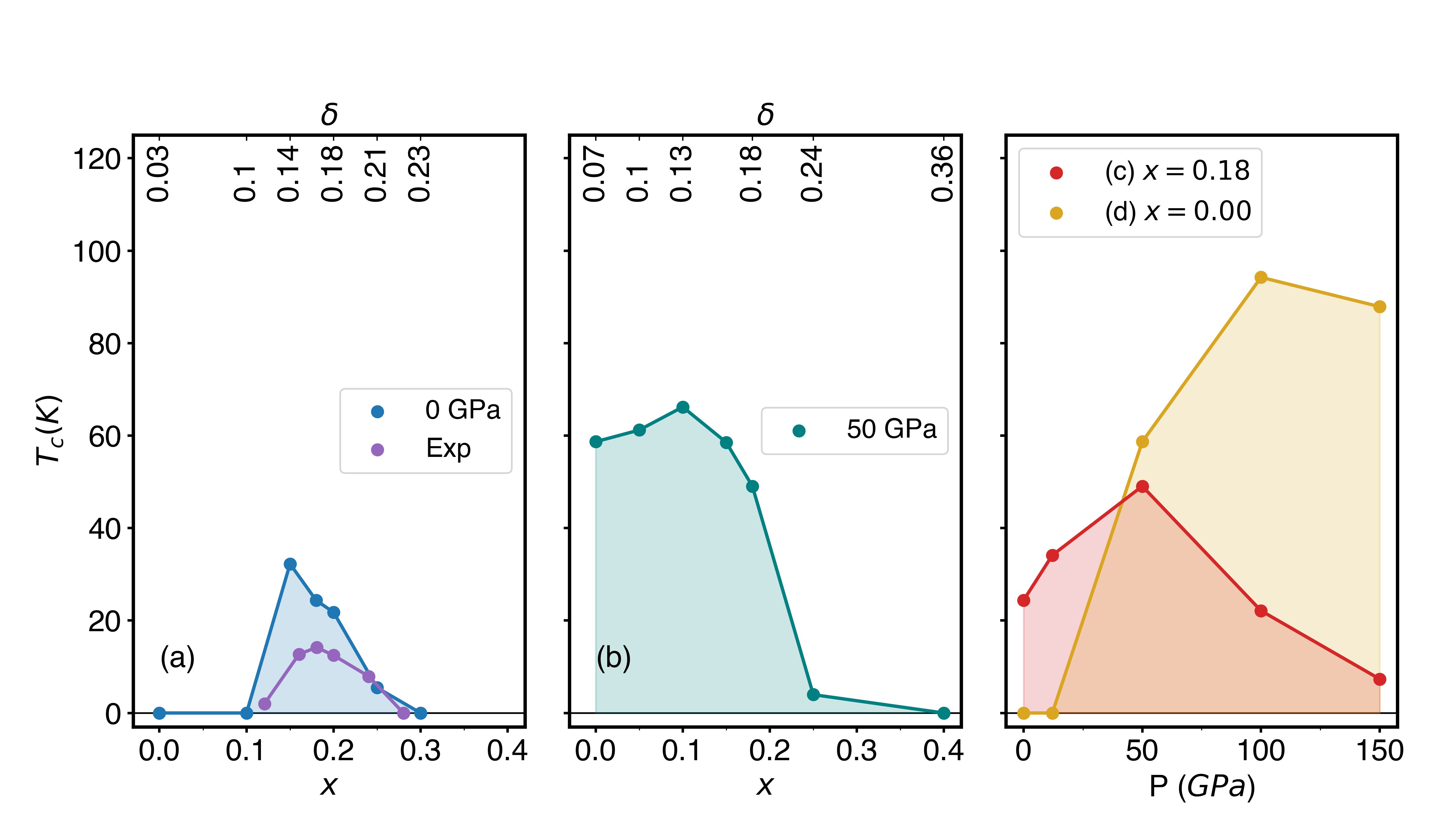
Figure 1: Phase diagram $T_{\text{c}}$ vs. Sr-doping $x$ and pressure $P$ of Sr_xPr_1-xNiO₂ as calculated in D$\Gamma$A. Four different paths are considered: as a function of $x$ for (a) 0 GPa and (b) 50 GPa; as a function of $P$ at (c) $x=0.18$ and (d) $x=0$. The secondary (upper) $x$-axis of panels (a), (b) shows the effective hole doping $\delta$ of the Ni $d_{x^{2}-y^{2}}$ orbital with respect to half filling. Panel (a) also compares to the experimental result from Ref. [9] (purple dots).

In this work, we employ the same state-of-the-art scheme that was so successful in Ref. [2], which is based on density functional theory (DFT), dynamical mean-field theory (DMFT), and the dynamical vertex approximation (D$\Gamma$A). We study the pressure dependence of the superconducting phase diagram of PrNiO₂ (PNO) with and without Sr doping. We find (i) a strong increase of the hopping $t$, almost by a factor of two, when going from 0 to 150 GPa, while the value of $U$, obtained through constrained random-phase approximation (cRPA), remains essentially unchanged as in cuprates [22]. Importantly, pressure further results in (ii) deeper electron pockets, effectively increasing the hole doping $\delta$ of the Ni $d_{x^{2}-y^{2}}$ band with respect to half-filling. Altogether, this results in the phase diagrams shown in Fig. 1, the main result of our work. When going from (a) ambient pressure to (b) 50 GPa, $T_{\text{c}}$ increases by up to a factor of two and $d$-wave superconductivity is observed in a much wider doping range – quite remarkably even without Sr doping. As a function of pressure, at doping fixed to $x=0.18$ (c), the simulated phase diagram shows a very similar increase of $T_{\text{c}}$ from 0 to 12 GPa as in experiment [13]. The figure further reveals that $T_{\text{c}}$ will continue to increase up to 49 K at 50 GPa, followed by a rapid decrease at higher pressures. For the parent compound, PrNiO₂ ($x=0$, d), the enhanced self-doping alone is sufficient to turn it superconducting with a maximum predicted $T_{\text{c}}$ of close to 100 K at 100 GPa.

II Results

As the superconducting nickelate films are grown onto a STO substrate, particular care has to be taken when simulating the effect of isotropic pressure in the diamond anvil cell (cf. Supplemental Material (SM) [37] Section LABEL:supp:subsect:methods_workflow for a flowchart of the overall calculations and Section LABEL:supp:subsect:methods_relaxation for further details of the pressure calculation). First, since the thickness of the film is 10-100 nm and thus negligible compared to that of the STO substrate, we calculate the STO equation of state in DFT and, from this, obtain the STO lattice parameters under pressure. Second, we fix the in-plane $a$ (and $b$) lattice parameters to that of STO under pressure and find the lattice parameter $c$ for the nickelate which minimizes the enthalpy at the given pressure. The resulting lattice constants are shown in Table 1. This procedure better reflects the response of the system to the rather isotropic pressures realized in experiment and is more realistic than that used in Ref. [7] where the $a$-$b$ lattice parameters had been fixed to that of unpressured STO [7].

$P$	$a$	$c$	$t$	$t^{\prime}$	$t^{\prime\prime}$
[GPa]	[Å]	[Å]	[eV]	[eV]	[eV]
0	3.90	3.32	-0.39	0.10	-0.05
12.1	3.83	3.20	-0.42	0.10	-0.05
50	3.67	3.03	-0.48	0.11	-0.06
100	3.54	2.89	-0.56	0.11	-0.07
150	3.45	2.79	-0.62	0.12	-0.07

Table 1: Ab initio values for the lattice constants and the hoppings of the 1-orbital Hubbard model for PrNiO₂ under pressure. Here, $t$, $t^{\prime}$, and $t^{\prime\prime}$ are the nearest, next-nearest, and next-next-nearest neighbour $d_{x^{2}-y^{2}}$-hoppings.

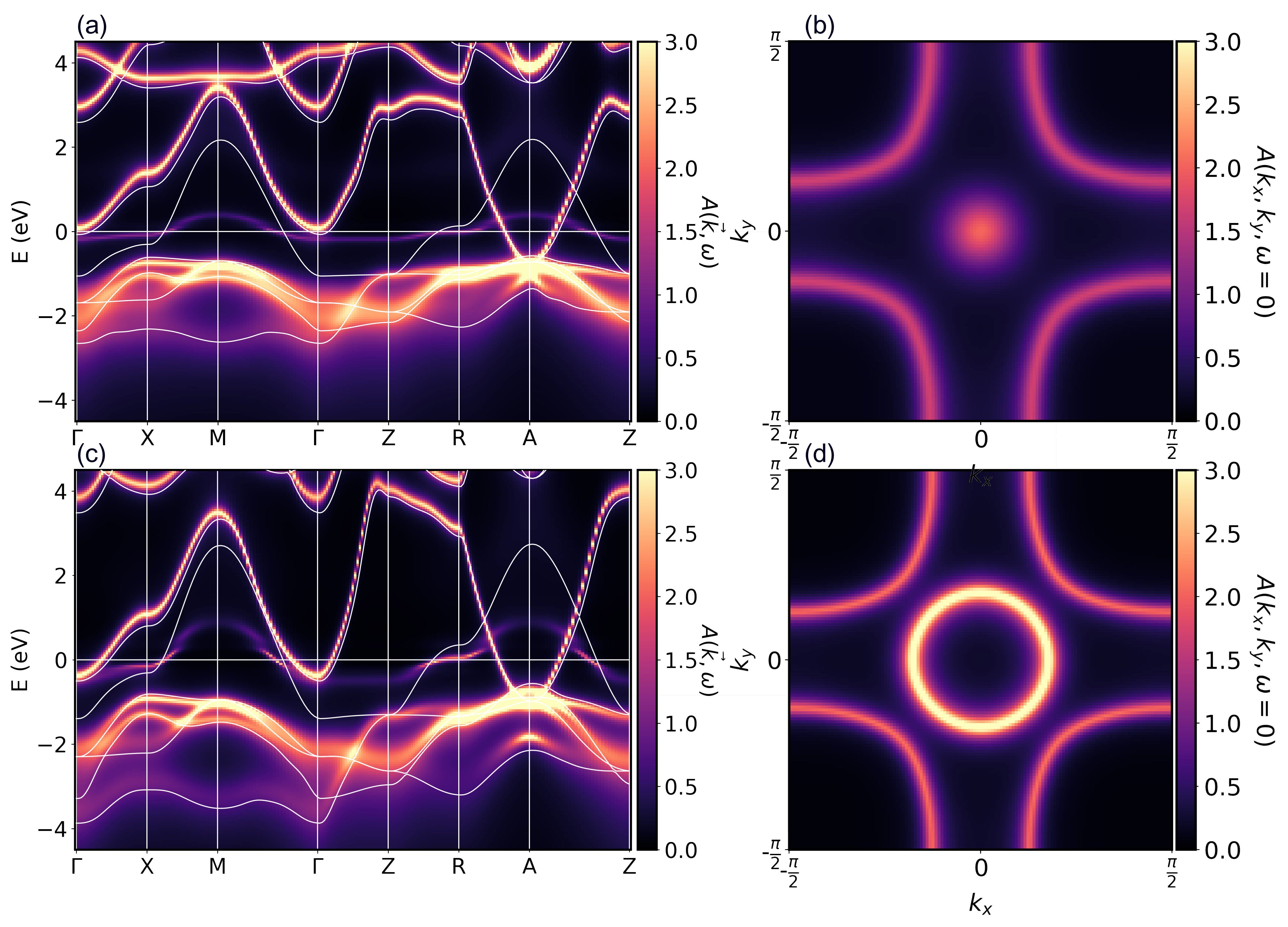
Figure 2: Spectral function for undoped PNO. Panels (a) and (c) show the DMFT spectral function $A(\textbf{k},\omega)$ (color scale) and the Wannier bands (white lines) along a path through the Brillouin zone at temperature $T=300K$. Panels (b) and (d) show the same spectral function in the $k_{z}=0$ plane. $A(k_{x},k_{y},k_{z}=0,\omega=0)$. The $\Gamma$ point is at the center, i.e. $(k_{x}=0,k_{y}=0)$.

With the crystal structure determined, we calculate the DFT electronic structure at pressures of 0, 12, 50, 100, and 150 GPa. Next, we perform a 10- and 1-orbital Wannierization around the Fermi energy, including all Pr-$d$ plus Ni-$d$ orbitals and only the Ni $d_{x^{2}-y^{2}}$ orbital, respectively. The DFT band structures and Wannier bands are shown in SM  [37] Fig. LABEL:supp:fig:wannier_pressure and as white lines in Fig. 2.

Following the method of Refs. [2, 29], we supplement the Wannier Hamiltonian with a local intra-orbital Coulomb interaction of $U=4.4\,$eV (2.5 eV) and Hund’s exchange $J=0.65\,$eV (0.25 eV) for Ni-3$d$ (Pr-5$d$) as calculated in cRPA [24]. For the thus derived 10-band model we perform DMFT calculations. The resulting DMFT spectral function of undoped PNO is shown in Fig. 2, for 0 and 50 GPa. We see that the Ni $d_{x^{2}-y^{2}}$ orbital crossing the Fermi energy is strongly quasiparticle-renormalized compared to the DFT result (white lines). In addition, there are pockets at the $\Gamma$ and A momenta, which essentially follow the DFT band structure without renormalization.

Important for the following is that, with the overall increase of bandwidth under pressure, the size of the pockets grows dramatically under pressure in DFT and DMFT alike. The enlargement of the $\Gamma$ pocket can also be seen from the Fermi surface Fig. 2 (d) vs. (b). The effect at higher pressures is shown in SM  [37] Fig. LABEL:supp:fig:10_bands_0_doping_vs_pressure-LABEL:supp:fig:fs_pressure.

The results of the 10-band model show that the low-energy physics of the system boils down to one-strongly correlated Ni $d_{x^{2}-y^{2}}$ orbital plus weakly correlated electron pockets. Here, the A-pocket does not hybridize by symmetry with the Ni $d_{x^{2}-y^{2}}$ band, as is evident by the mere crossing of both between R and A. The band forming the $\Gamma$ pocket, on the other hand, mainly hybridizes with other Ni orbitals that in turn couple to the Ni $d_{x^{2}-y^{2}}$ through the Hund’s $J$. Note, however, that the main spectral contribution of these other Ni-$d$ orbitals is still well below the Fermi energy in Fig. 2.

The above justifies a one-band minimal model for superconductivity in PNO [2, 30, 13], with the working hypothesis that superconductivity arises from the correlated Ni $d_{x^{2}-y^{2}}$ band only. However, the effective hole-doping $\delta$ of the Ni $d_{x^{2}-y^{2}}$ band (relative to half-filling) has to be calculated from the 10-band DFT+DMFT to properly account for the electrons in the pockets. In the following, it is thus imperative to always distinguish between the number of holes corresponding to Sr substitution of the Pr site (chemical doping $x$) and the holes in the Ni $d_{x^{2}-y^{2}}$ band compared to half filling (effective doping $\delta$).

The electron pockets induce a nonlinear dependency of $\delta$ from $x$, and their growth with pressure $P$ causes $\delta$ to increase by about 0.06 from 0 to 100 GPa, see SM [37] Fig. LABEL:supp:fig:pressure_eff_filling.

Using the effective doping $\delta$ of the Ni $d_{x^{2}-y^{2}}$ band, we perform a second DMFT calculation for the single Ni $d_{x^{2}-y^{2}}$ orbital, which we describe as a single-band Hubbard model with an interaction of $U=3.4\,$eV. This $U$ is smaller than for the 10-band model due to additional screening, but it is notably insensitive to pressure (cf. SM [37] Tab. LABEL:supp:tab:U). The main effect of pressure is instead the increase of $t$ as summarized in Table 1 and the already mentioned enhanced self-doping.

In Fig. 3, we show the spectral function $A(\textbf{k},\omega)$ of the 1-band model for PNO as a function of pressure and $x=0$. The panels for 0  and 50 GPa can be compared to Fig. 2 (a,c) and show that the 1-band model reproduces the renormalization of the Ni $d_{x^{2}-y^{2}}$ orbital in the fully-fledged 10-band calculation.

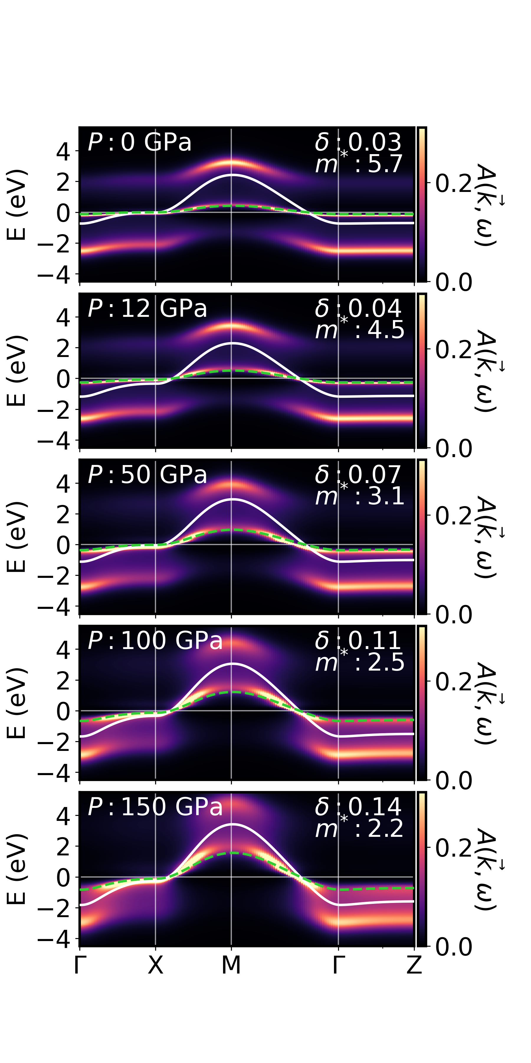
Figure 3: DMFT spectral function (color bar) for undoped PNO for the 1-band model and as a function of pressure from 0 to 150 GPa at $T=0.0125t$. The original DFT Wannier band and the same band renormalized with the effective mass are shown as solid white and dashed green lines, respectively.

Hubbard bands are visible at all pressures in Fig. 3, but become more spread out and less defined with increasing pressure. Simultaneously, the effective mass $m^{*}$ decreases, and the bandwidth widens. Similar results but for the experimentally investigated Sr-doping $x=0.18$ can be found in SM [37] Fig. LABEL:supp:fig:spfun_d_0.18_pressure, and as a function of doping at 50 GPa in Fig. LABEL:supp:fig:spfun_doping_50_GPa.

Next, we calculate the superconducting $T_{\text{c}}$ using D$\Gamma$A [32, 29]. In Fig. 1, we follow four different paths in parameter space: as a function of doping at (a) 0 GPa and (b) 50 GPa as well as as a function of pressure with Sr-doping (c) $x=0.18$, i.e., for the parent compound, and (d) $x=0$. At ambient pressure in Fig. 1 (a) our results are in excellent agreement with our previous calculations for other nickelates [2, 30], cf. SM [37] Fig. LABEL:supp:fig:tc_and_t_p. The small differences are ascribable to the slightly different material, and are in good agreement with experiment [3, 15]. We find the effect of pressure to be significant: At 50 GPa, the maximum $T_{\text{c}}$ is enhanced by a factor of two compared to ambient pressure, while the maximum slightly shifts to lower doping ($x=0.10$). Remarkably, even the undoped parent compound becomes superconducting at 50 GPa [$x=0$ in Fig. 1 (b)], due to the increased self-doping from the electron pockets.

The experimental Sr-doping of $x$=0.18 [41] is close to optimal doping at 0 GPa. Increasing pressure in Fig. 1 (c), we observe an increase of $T_{\text{c}}$ by 0.81 K/GPa in excellent agreement with the experimental rate of 0.96 K/GPa [41], for pressures up to 12 GPa. The predicted $T_{\text{c}}$ of 30 K at 0 GPa is slightly higher in theory than the experimental 18 K [41], but still in good agreement. As pressure increases beyond 12 GPa, $T_{\text{c}}$ continues to grow and peaks at around 50 GPa with 49 K, before decreasing for higher pressures.

Most striking is the result for the undoped compound PNO in Fig. 1 (d). Here, superconductivity sets in below 50 GPa and peaks at almost 100 K around 100 GPa. Intrinsic doping from the electron pockets is sufficient to make the parent compound superconducting at high temperature.

III Discussion

To rationalize our results, we plot the four paths at fixed pressure, respectively, fixed Sr-doping $x$ in Fig. 4, but now as a function of $U/t$ and the effective hole doping $\delta$ of the Ni $d_{x^{2}-y^{2}}$ orbital. Superimposed is the D$\Gamma$A superconducting eigenvalue $\lambda$ [30], with the darker gray regions corresponding to a higher $T_{\text{c}}$.

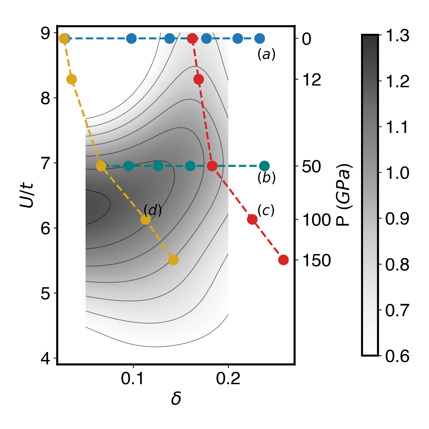
Figure 4: The considered four paths in the $U/t$ vs. effective hole doping $\delta$ parameter space: at a fixed pressure of (a) 0 GPa and (b) 50 GPa as a function of Sr-doping $x$; as a function of pressure for fixed Sr-doping (c) $x=0.18$ and (d) $x=0.00$. The gray color bar indicates the strength of superconductivity (superconducting eigenvalue $\lambda$ at $T=0.01$t; from [30]). The secondary $y$ axis reports the pressure corresponding to the $U/t$ values shown.

The application of an isotropic pressure on infinite-layer PrNiO₂ has two effects: First, it boosts the hopping $t$ of the Ni $d_{x^{2}-y^{2}}$ orbital, which at 150 GPa becomes almost twice as large than at 0 GPa, see Table 1. This increases the overall energy scale and thus enhances $T_{\text{c}}$. Since $U$ does not change significantly, the ratio $U/t$ also decreases. This is preferable for superconductivity since at ambient pressure PNO exhibits a $U/t$ slightly above the optimum of $U/t\sim 6$ (above the darker gray region in Fig. 4). However, at high pressures of e.g. 100 GPa and 150 GPa curves (c) and (d) have passed the optimum in Fig. 4; $T_{\text{c}}$ in Fig. 1 decreases again.

Second, pressure enhances the effective hole doping $\delta$ even at fixed Sr-doping $x$, as the electron pockets become larger. For this reason, curves (c) and (d) in Fig. 4 deviate from a vertical line. For Sr-doping (c) $x=0.18$, which is close to optimum at 0 GPa, the curve moves away from optimum doping to the overdoped region when pressure is applied. This is a major driver for the decrease of $T_{\text{c}}$ above 50 GPa in Fig. 1 (c). In stark contrast, for the parent compound ($x=0$; d) the effective hole doping $\delta$ goes from underdoping to optimal doping, and only at much larger pressures to overdoping and too small $U/t$. Consequently, PNO without doping hits the sweet spot for superconductivity in Fig. 4 at a pressure between 50 and 100 GPa.

IV Conclusion

In short, our results strongly suggest that experiments for infinite-layer nickelates are still far from having achieved their maximum $T_{\text{c}}$. Surprisingly, the maximum $T_{\text{c}}$ of almost 100 K is predicted to be found in undoped PrNiO₂ between 50 and 100 GPa. This places nickelates almost on par with cuprates in the Olympus of high-$T_{\text{c}}$ superconductors. The nickelate phase diagram under pressure will not only exhibit a significant increase in $T_{\text{c}}$ but also a wider dome. In particular, the maximum of this dome is shifted to lower Sr-doping $x$ when a pressure of 50 - 100 GPa is applied.

Such pressures can be achieved experimentally in diamond anvil cells. An alternative route to obtain the same in-plane lattice compression is using a substrate with smaller lattice parameters. For example, LaAlO₃, YAlO₃ and LuAlO₃ have lattice parameters of 3.788 Å [42], 3.722 Å [43] and 3.690 Å [44], respectively, which are already close to the in-plane lattice constants at 50 GPa. As this approach would not change the out-of-plane lattice parameter, the self-doping of the Ni $d_{x^{2}-y^{2}}$ band from the electron pockets should be less important. Hence we expect that with these substrates a higher $T_{\text{c}}$ might be achieved, but only with at least 10% doping.

V Methods

In this section, we summarize the computational methods employed. The interested reader can find additional information in the Supplementary Material [37], and data and input files for the whole set of calculations in the associated data repository [1].

Density functional theory calculations were performed using the Vienna ab-initio simulation package (VASP) [3, 5] using projector-augmented wave pseudopotentials and Perdew-Burke-Ernzerhof exchange correlation functional adapted for solids (PBESol) [48, 4], with a cutoff of 500 eV for the plane wave expansion. Integration over the Brillouin zone was performed over a grid with a uniform spacing of 0.25 $\AA^{-1}$ and a Gaussian smearing of 0.05 eV. Wannierization was performed using wannier90 [18].

The Hubbard $U$ of the 1-orbital setup under pressure was computed from first principles using the constrained random phase approximation (cRPA) in the Wannier basis [19] for entangled band-structures [20], relying on a DFT electronic structure obtained from a full-potential linearized muffin-tin orbital method [21].

DMFT calculations were performed using w2dynamics [28], with values of $U$, $J$, and $t$ as detailed in the main text, and in Tab. LABEL:supp:tab:summary_dmft_inputs and SM [37] Tab. LABEL:supp:tab:10band_DMFT. The 10-band calculations were performed at a temperature of 300 K, with a total of 30 iterations to converge the local Green’s function, and a final step with higher sampling. The 1-band DMFT calculations were performed at variable temperature, with a total of 70 iterations, and a final step with higher sampling, which was increased at lower temperatures.

The calculation of the non-local quantities via ladder D$\Gamma$A and the solution of the linearized Eliashberg equation was performed starting from the local vertex calculated with w2dynamics using our own implementation, available upon reasonable request.

Author Contributions

S. D. C. performed the DFT, and DMFT calculations. S. D. C. and P. W. performed the D$\Gamma$A calculations. J. M. T. performed the cRPA calculations. L. S. and K. H. designed and supervised the project. All authors participated in the discussion, contributed to the writing of the manuscript, and approved the submitted version.

Competing interests

The authors declare that they have no competing interests.

Data and materials availability

The raw data for the figures reported, along with input and output files is available at [1]. Related data including the local Green’s functions and DFT calculations are also available in the NOMAD repository [55, 56].

Supplementary Information:
Unconventional superconductivity without doping: infinite-layer nickelates under pressure

This Supplemental information contains additional information on the methods employed in Section VI and additional results in Sections VII. Specifically, Section VI.1 provides an overview; Section VI.2 gives details of the density functional theory (DFT) calculation; Section  VI.3 gives details of the structural relaxation; Section  VI.4 gives details on the Wannierization of the DFT bands at the different pressures. Section  VI.5 provides information on the constrained random phase approximation (cRPA) calculation of the interaction parameters; Section  VI.6 gives further details on the dynamical mean-field theory (DMFT) calculations; and Section VI.7 on the dynamical vertex approximation (D$\Gamma$A). Additional results are presented in Section VII. This includes DFT+DMFT calculations for the 10- and 1-band model in Section VII.1, a comparison of the D$\Gamma$A $T_{\text{c}}$ to that of Sr_xNd_1-xNiO₂ in Section VII.2, and an in-depth test of the virtual crystal approximation (VCA) in Section VII.3.

February 27, 2024

VI Methodological details

In this section, we provide a more detailed description of the methods employed in the main text. The interested reader can find the input files for the whole set of calculations in the associated data repository [1].

VI.1 Complete workflow

We start with presenting a flowchart of the entire methodology as an overview in Fig. S1; and further details on the individual steps can then be found in the subsequent Sections.

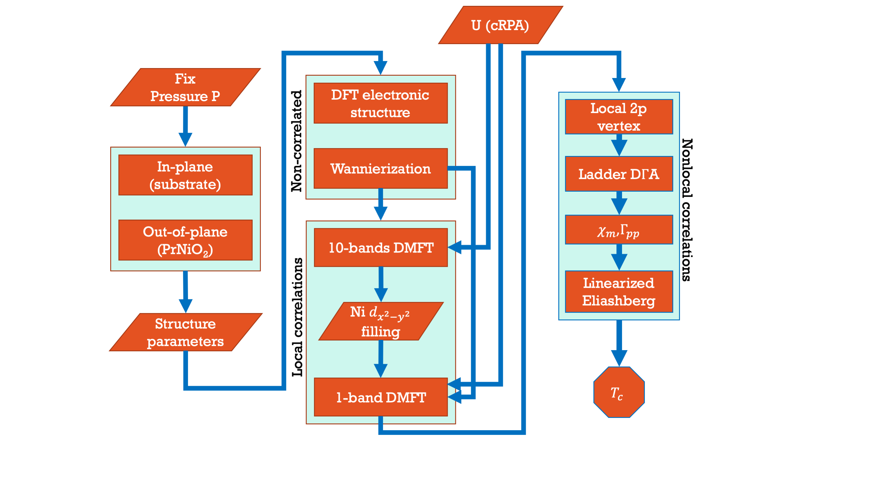
Figure S1: Flowchart summarizing the whole workflow employed in the project.

We start by computing the in-plane lattice parameter as a function of pressure from the STO equation of state in DFT and fix the PNO in-plane lattice parameters to that of the substrate. Next, we determine the out-of-plane lattice parameter of PNO, as detailed in VI.3. From the relaxed crystal structure, we compute the electronic dispersion $\epsilon_{\textbf{k}}$ using Density Functional Theory and extract the Wannier functions for 10 bands (Ni-$d$ + Pr-$d$) and 1 band (Ni $d_{x^{2}-y^{2}}$).

As described in Ref. [2], we first perform a DMFT calculation for the 10 bands case, which allows us to obtain the filling of the Ni $d_{x^{2}-y^{2}}$ in the case of interacting Ni and Nd orbitals. The values of interaction employed in this calculation are reported in Table 3. Using the thus computed filling of the Ni $d_{x^{2}-y^{2}}$ band, we perform a second DMFT calculation for the single Ni $d_{x^{2}-y^{2}}$ band, from which we obtain the local two-particle Green’s function $G^{(2)}(i\nu,i\nu^{\prime},i\omega)$.

Finally, using ladder-D$\Gamma$A we compute the non-local vertex and the (magnetic) susceptibility at various temperature. The superconducting $T_{\text{c}}$ is then estimated as the temperature for which the leading eigenvalue of the linearized Eliashberg equation is equal to one, as in Ref. [2].

VI.2 Density Functional Theory

DFT calculations are performed with the Vienna ab-initio Simulation Package (VASP) [3], using the Perdew-Burke-Ernzerhof adapted for solids (PBESol) [4] exchange-correlation functional. We employ the projector-augmented waves (PAW) pseudopotentials provided within the VASP package [5], for which praseodymium is constructed with $f$ orbitals frozen within the core states. Integration over the Brillouin zone was performed over a uniformly-spaced grid with a spacing of 0.25 Å^-1, and a Gaussian smearing of 0.05 eV. The input and output files for all calculations performed are available as additional data [1].

At the DFT level, the Sr-doping of the PrNiO₂ crystal was simulated by means of the virtual crystal approximation (VCA) to simulate a virtual Pr_1-xSr_x atom following the method describe by Bellaiche and Vanderbilt [6], and implemented in VASP. The use of this approximation, despite the different core of Sr and Pr is justified by the fact that in the system studied both, Pr and Sr, act mostly as charge donors and spacers between NiO₂ planes, and do not contribute significantly to the states at the Fermi energy. Nevertheless, we checked extensively the quality of the VCA against Vergard’s law, and on the structural and electronic properties of Pr_0.75Sr_0.25NiO₂, compared with the results on a 2$\times$2$\times$2 supercell. As these checks are quite extensive and we do not want to interrupt the further discussion of the workflow here, we present in Section VII.3, Figures S15 (Vergard’s law) and S16 (comparison with 2$\times$2$\times$2 supercell). This aspect of Figure S4, which we present already in Section VI.3 for its information on how to obtain the $c$-axis parameter, is also discussed in Section VII.3. All these tests confirmed that the VCA is consistent with the results obtained for supercells in the structure studied.

VI.3 Structural Relaxation

In this section, we report the main results for the structural relaxation of the SrTiO₃ (STO) substrate. In Fig. S2 we show the equation of states along with the results from a fit with the Birch-Murnaghan equation for STO as a function of pressure. In Fig. S3 we show the corresponding lattice parameter.

The effect of isotropic pressure was computed in two steps, including the effect of the SrTiO₃ (STO) substrate on the in-plane lattice parameter, as well as the effect of pressure on the $c$ axis. This strategy differs substantially from Ref. [7], where the in-plane lattice constant is kept constant, as it is not suited to study the rather isotropic pressures that are realized in experiments using diamond anvil cells.

Our method of computing the crystal structure of Pr_1-xSr_xNiO₂, on the other hand, is motivated by the consideration of how the actual crystal is grown in experiments. Infinite-layer nickelates are grown over a perovskite substrate. Often STO is used [8, 9, 10, 11, 12], this also includes the experiments by Wang et al. [13] which motivated the present study. But, NdGaO₃ (NGO) [14] and (LaAlO₃)_0.3(Sr₂TaAlO₆)_0.7 (LSAT) [15] was employed as well. The nickelate layer is grown with a thickness between 10 and 100 nm [14, 8, 9, 11, 10, 12, 16] over a bulk substrate which can be regarded as infinite, and capped again with a few layers of the same substrate. Hence we work in the hypotheses that:

1. The nickelate is forced to assume the same in-plane lattice constant of the substrate on which it is grown.

2. In the $xy$ plane the elastic response of the system is dominated by the substrate, due to the substrate being much thicker.

3. Along the $z$ direction, the nickelate is not constrained by the substrate, hence its response is independent from it.

The above is then modelled in the two following steps:

1. We compute the equation of state for bulk STO in the cubic phase. At a given pressure, the equation of state is used to extract the in-plane lattice constants $a=b$ (Supplementary Figure S2).

2. With $a$ and $b$ fixed to the value given by STO at the chosen pressure, we compute the enthalpy of the nickelate phase as a function of the $c$ axis, see Fig. S4. The $c$ value that minimizes the enthalpy corresponds to the equilibrium value.

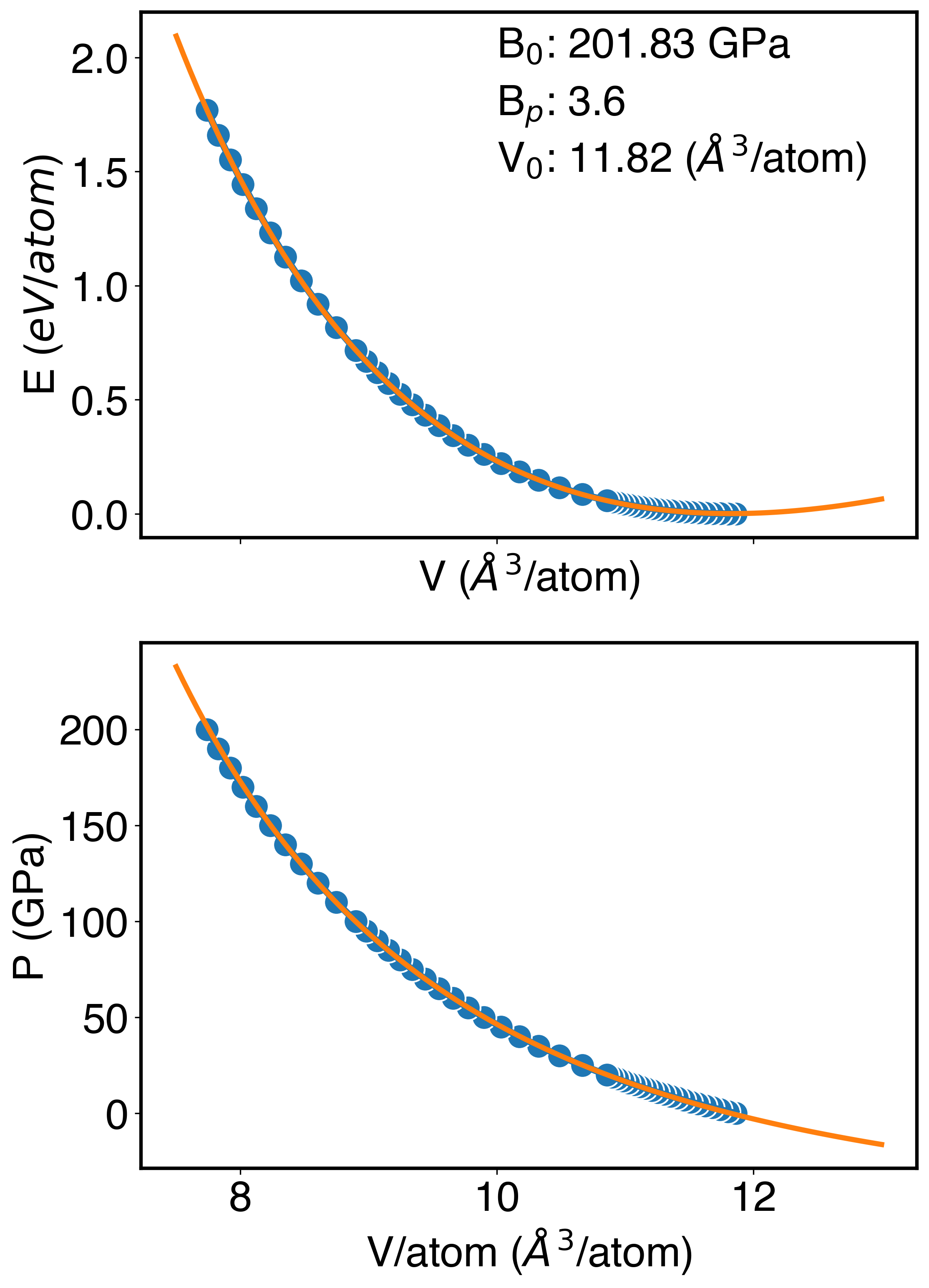
Figure S2: Equations of state $E(V)$ and $P(V)$ for SrTiO₃ from 0 to 200 GPa. The blue dots and the orange line denote the values computed within Density Functional Theory and the fit, using the Birch-Murnaghan equation of state [17]. In addition, we report the results of the curve fit.

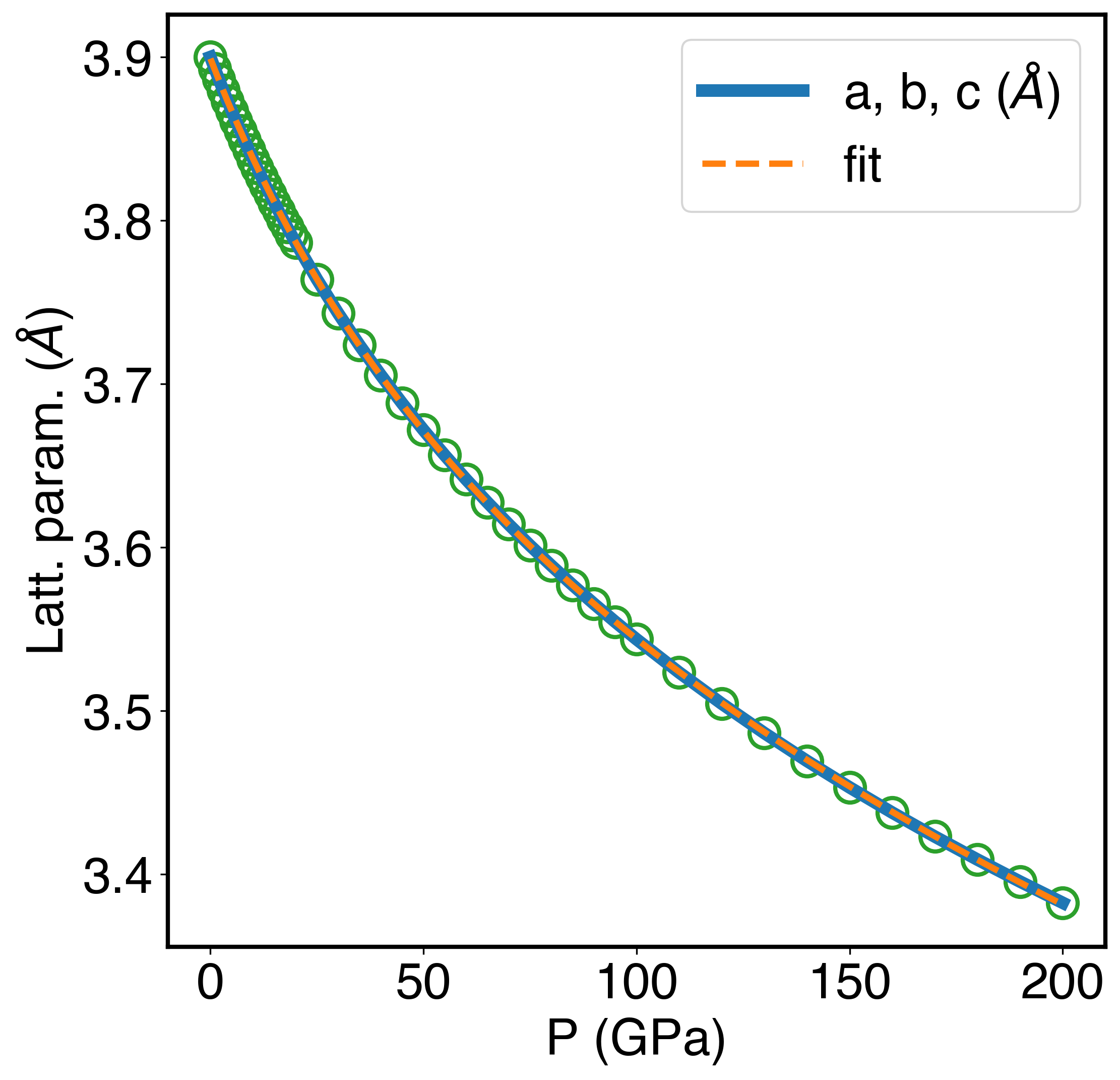
Figure S3: Lattice parameter of STO as a function of pressure from our DFT calculations.

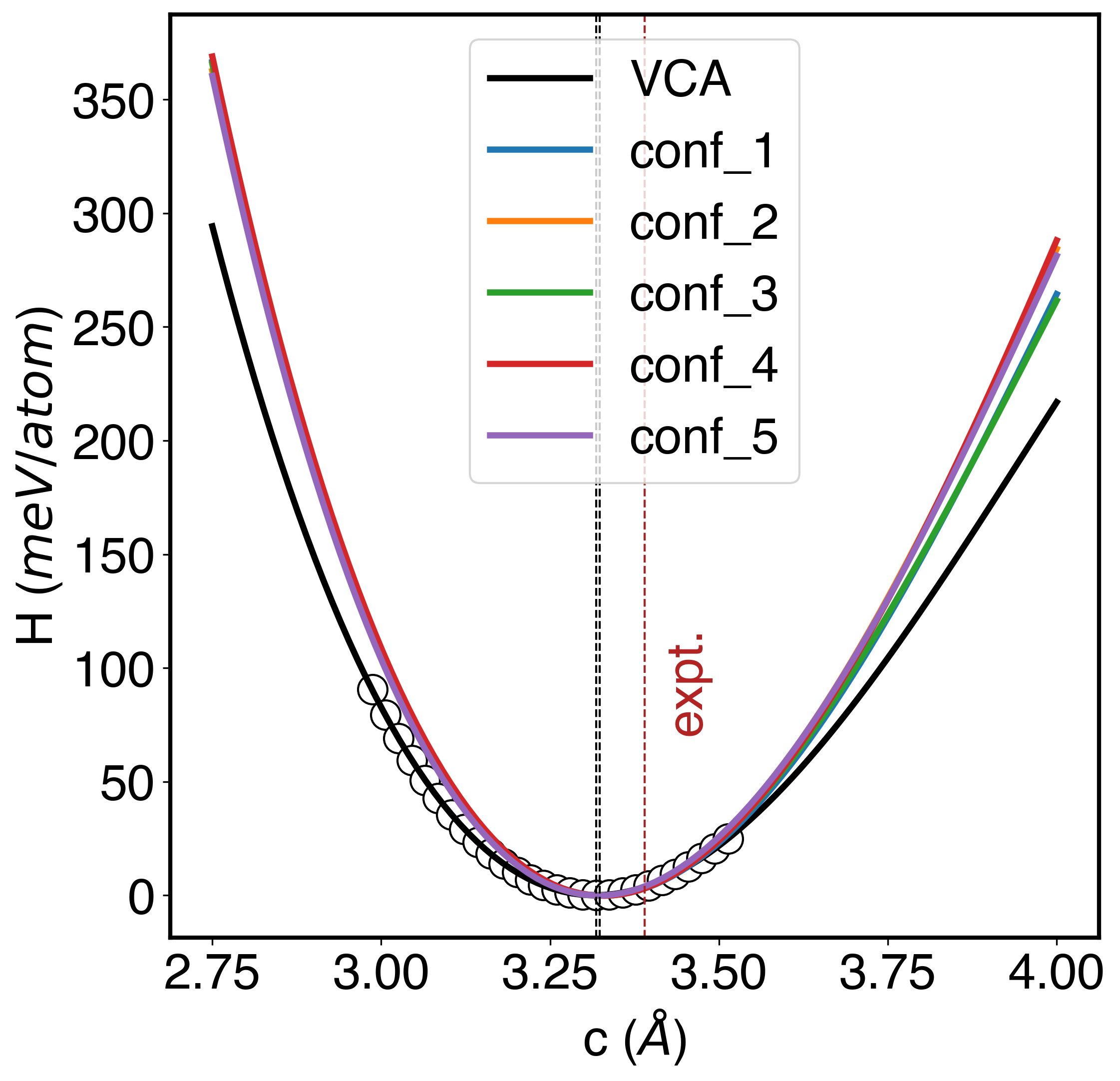
Figure S4: Enthalpy versus value of the $c$ axis for Pr_0.75Sr_0.25NiO₂ using the VCA and in five different supercells. The VCA value is shown as a black line, and individual points are shown as black dots. The results for the supercells are shown as colored lines.

VI.4 Wannier Functions

The DFT bandstructure calculated in VASP is subsequently mapped onto a 10- and a 1-band Wannier basis using maximally localized Wannier orbitals and the wannier90 code [18]. Here, $d$ orbitals centered on Pr and Ni were used for the initial projections for the 10-bands calculations, and a single d${}_{x^{2}-y^{2}}$ orbital centered on Ni was used as initial projection for the 1-band calculation. The reader interested in the energy ranges for the disentanglement and frozen windows of each calculation can find the corresponding input files in [1]. The Hamiltonian $H(\textbf{k})$ was obtained as the Fourier transform of the wannier90 output.

Fig. S5 shows the direct comparison between Wannier and DFT bands. While there are some deviations of the 10-band model and the DFT band above the Fermi energy where additional bands –besides the 10-bands considered– cross, the agreement at low energies is excellent. And this is the relevant region for the subsequent DMFT calculation.

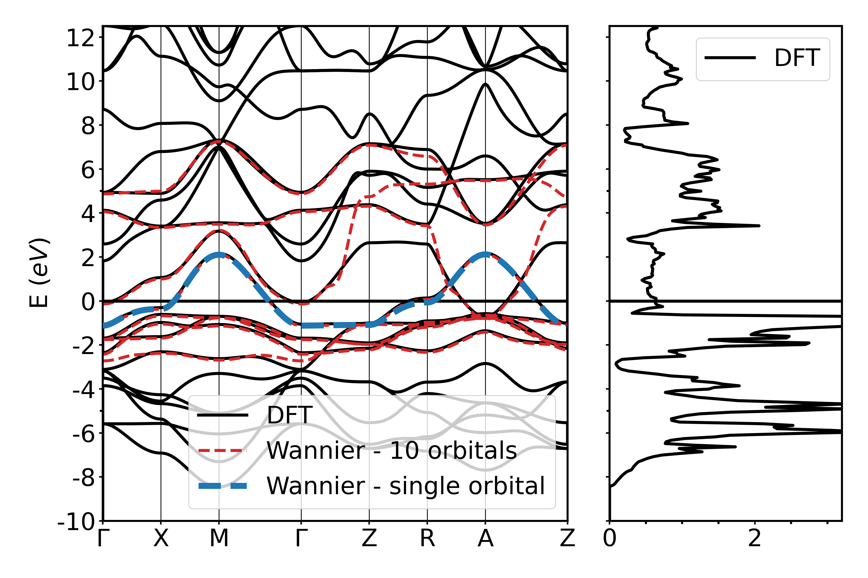
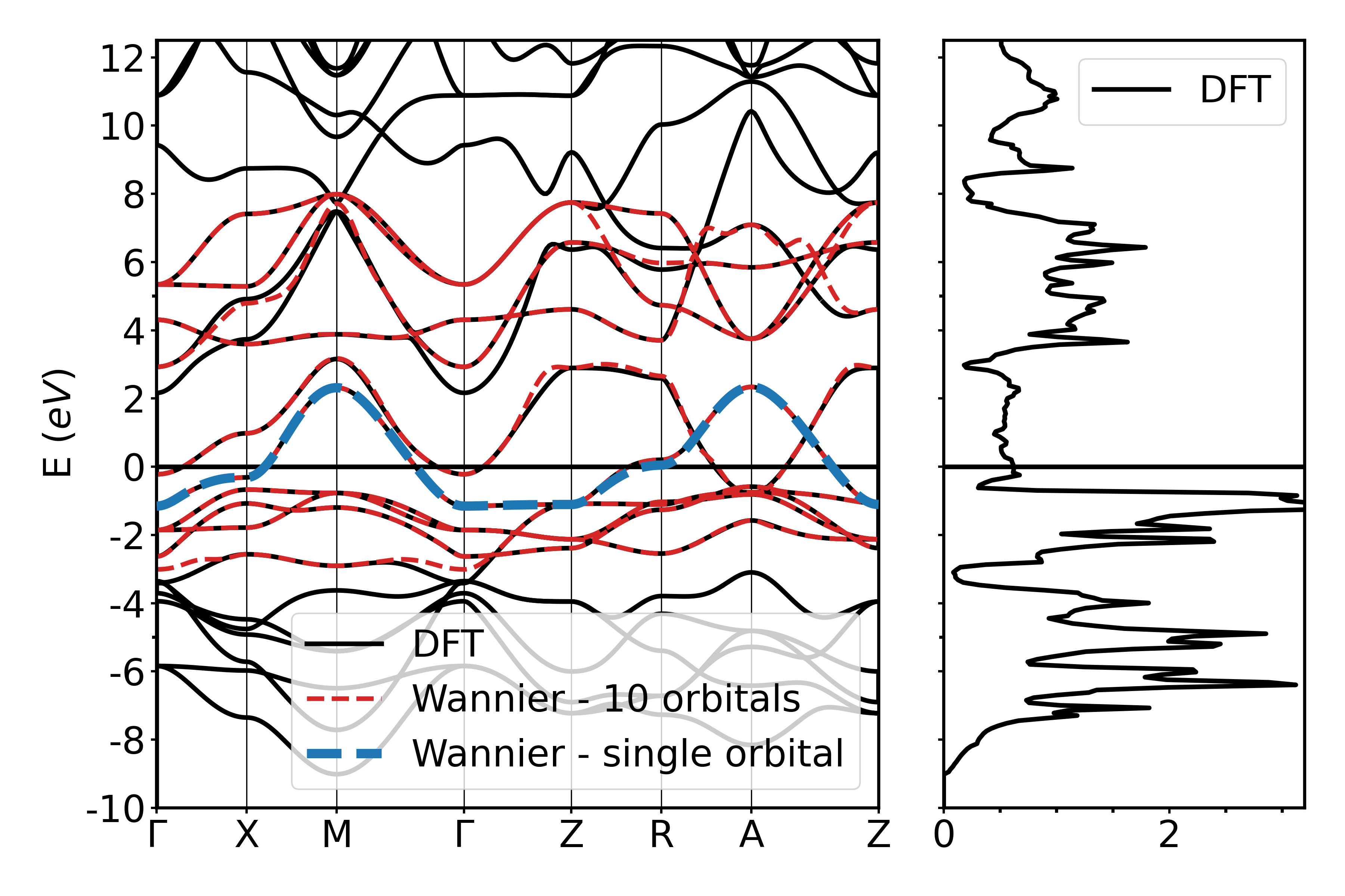
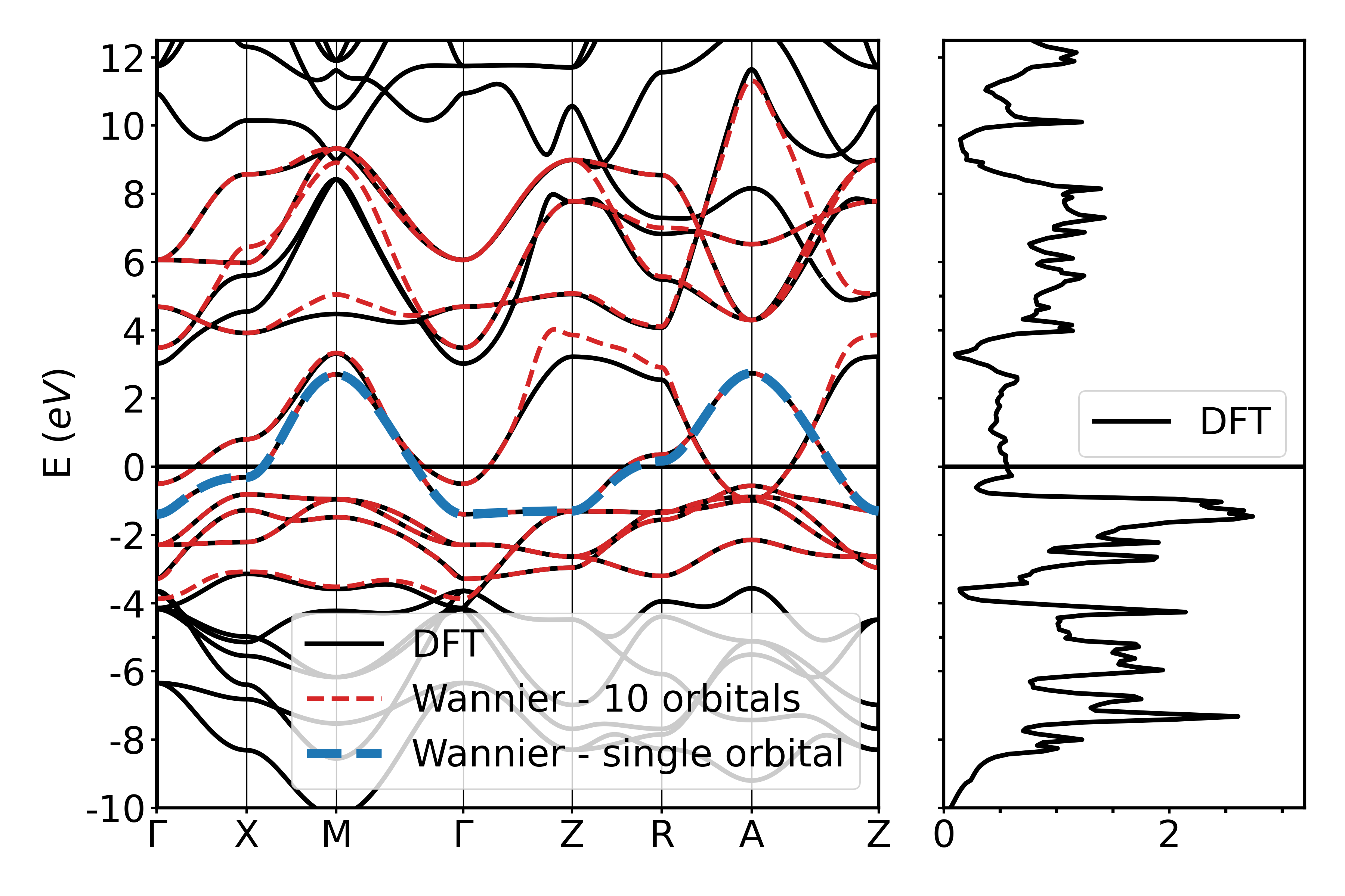
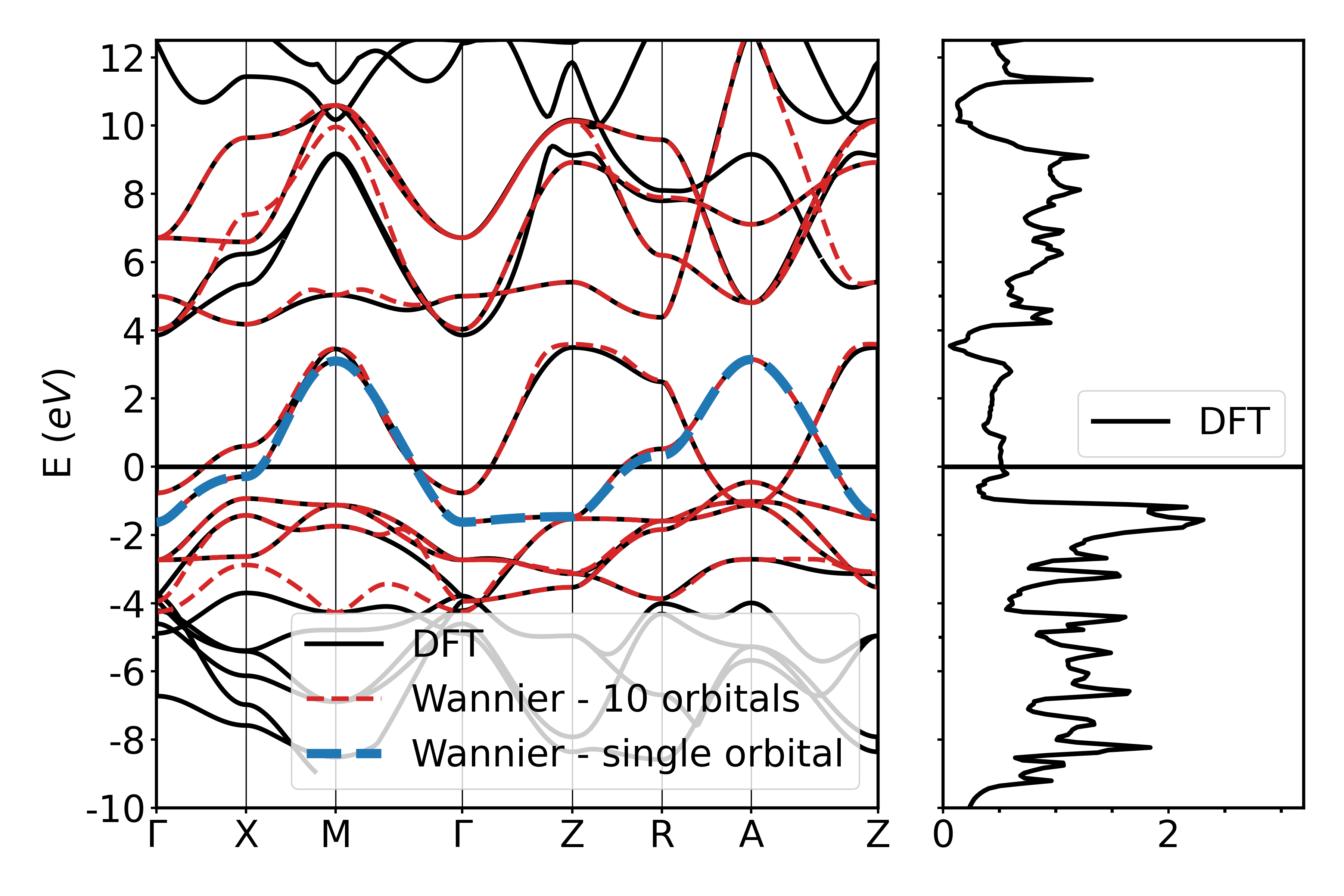
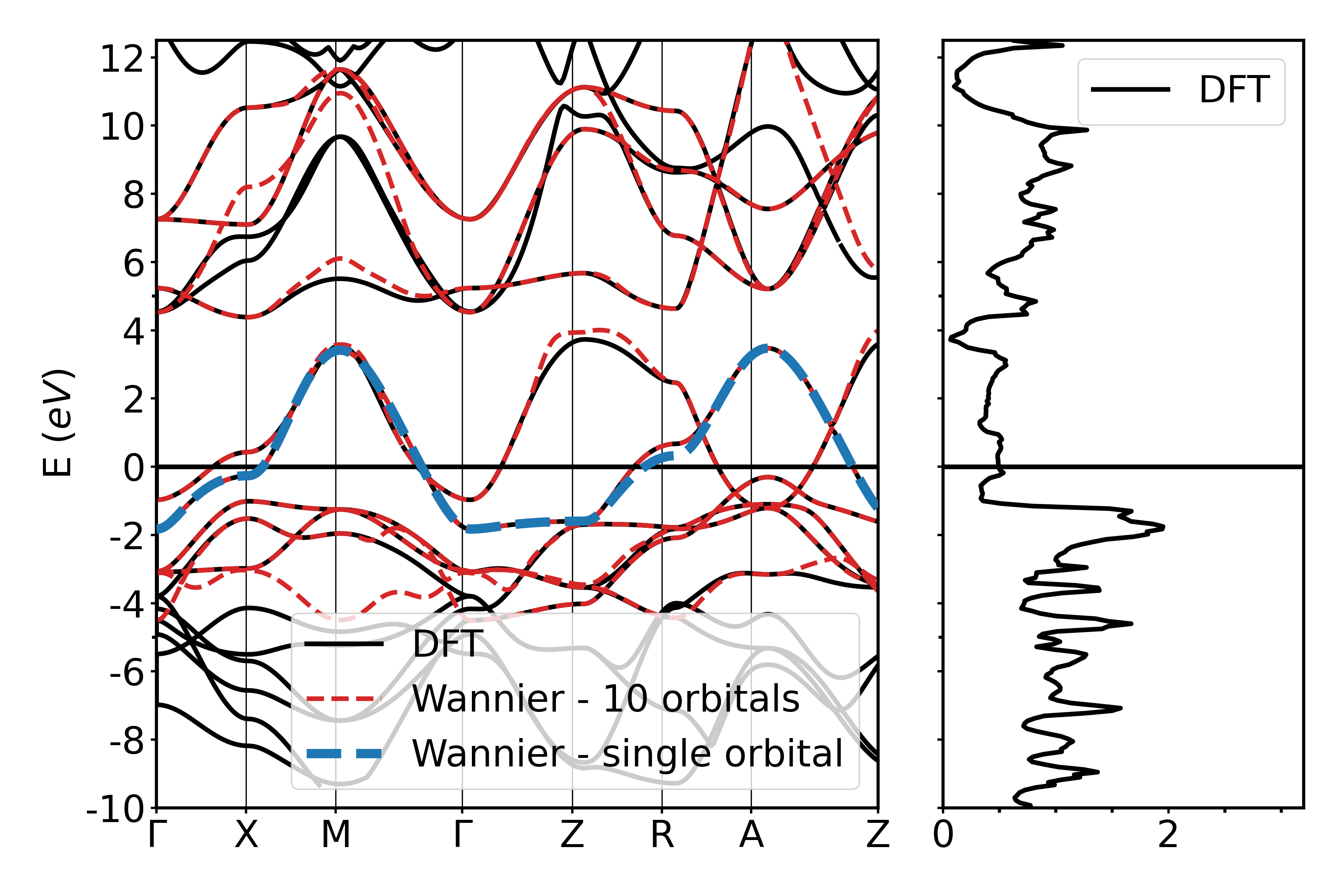
Figure S5: DFT electronic band structure and 10- and 1- band wannierization as a function of pressure. The DFT bands, the 10 bands wannierization and the 1 band wannierization are shown as black solid, red dashed, and blue dashed lines, respectively. The figures are shown in order of ascending pressure. From top left to bottom right: 0, 12, 50, 100, and 150 GPa, respectively.

From the wannierization, we can also extract the hopping amplitudes $t$, $t^{\prime}$, and $t^{\prime\prime}$ for nearest, next-nearest, and next-next-nearest neighbour hopping for the effective 1-orbital model. These parameters for different pressures and dopings are reported in Table 1 and serve as a DMFT input for the 1-band calculation. In case of the fully-fledged 10-band DMFT calculation, we used the full $H(\textbf{k})$ of the Wannier bands, without restriction to shorter-range hoppings.

Pressure	Doping	$t$	$t^{\prime}$	$t^{\prime\prime}$	U	U	neff Ni $d_{x^{2}-y^{2}}$
(GPa)		(eV)	(eV)	(eV)	(eV)	($t$)	($e/band$)
0	0%	-0.388	0.097	-0.049	3.4	8.77	0.973
12	0%	-0.416	0.099	-0.052	3.4	8.17	0.965
50	0%	-0.483	0.109	-0.059	3.4	7.04	0.933
100	0%	-0.558	0.112	-0.067	3.4	6.10	0.887
150	0%	-0.617	0.118	-0.073	3.4	5.51	0.858
0	18%	-0.388	0.097	-0.049	3.4	8.77	0.838
12	18%	-0.416	0.099	-0.052	3.4	8.17	0.831
50	18%	-0.483	0.109	-0.059	3.4	7.04	0.817
100	18%	-0.558	0.112	-0.067	3.4	6.10	0.775
150	18%	-0.617	0.118	-0.073	3.4	5.51	0.742
0	0%	-0.388	0.097	-0.049	3.4	8.77	0.973
0	10%	-0.388	0.097	-0.049	3.4	8.77	0.902
0	15%	-0.388	0.097	-0.049	3.4	8.77	0.862
0	20%	-0.388	0.097	-0.049	3.4	8.77	0.823
0	25%	-0.388	0.097	-0.049	3.4	8.77	0.790
0	30%	-0.388	0.097	-0.049	3.4	8.77	0.767
50	0%	-0.483	0.109	-0.059	3.4	7.04	0.933
50	5%	-0.483	0.109	-0.059	3.4	7.04	0.905
50	10%	-0.483	0.109	-0.059	3.4	7.04	0.872
50	15%	-0.483	0.109	-0.059	3.4	7.04	0.840
50	20%	-0.483	0.109	-0.059	3.4	7.04	0.802
50	25%	-0.483	0.109	-0.059	3.4	7.04	0.762
50	30%	-0.483	0.109	-0.059	3.4	7.04	0.722
50	40%	-0.483	0.109	-0.059	3.4	7.04	0.643

Table 1: Calculated quantities for the single-band Hubbard model of the Ni $d_{x^{2}-y^{2}}$ band at the pressures and physical Sr-doping values $x$ employed in this paper. The effective filling $n=1-\delta$ is reported.

VI.5 Constrained random phase approximation

This Wannier Hamiltonian needs to be supplemented by the Coulomb interaction. To this end, the static Hubbard interaction $U$ was computed from first principles using the constrained random phase approximation (cRPA) in the Wannier basis [19] for entangled band-structures [20]. Here, the underlying electronic structure was computed from DFT using a full-potential linearized muffin-tin orbital (fplmto) method [21] and the local density approximation, applied to bulk LaNiO₂ using the relaxed tetragonal structures from Sec. VI.3. The calculations use $10^{3}$ reducible k-points, and a muffin-tin radius (RMT) for Ni of 1.97 Bohr radii, except for $P=100$ GPa, where RMT=1.9. At $P=50$ GPa the difference in RMT changes $U$ by merely 0.4%. The cRPA results for the 1-band model are shown in Table 2. Note that the Hubbard $U$ can indeed display a non-trivial dependence on pressure [22]. E.g., in cuprates in-plane compression increases the local interaction in a $d_{x^{2}-y^{2}}$ setting [23].

We find both the screened and the bare interaction—$U$ and $V$—to be essentially insensitive to pressure: Both the localization of the $d_{x^{2}-y^{2}}$-derived Wannier function and the screening remain constant. This justifies keeping $U$ unchanged with pressure. To account for the frequency-dependence of $U$ in cRPA a slightly larger value is needed, and we use a fixed $U=3.4\,$eV as is stated in Table 1 was already employed in [2].

$P$ [GPA]	0	12.1	20	50	100
$U$ [ev]	2.88	2.88	2.88	2.96	2.93
$V$ [eV]	19.4	19.3	19.2	19.3	19.0

Table 2: Local Hubbard interaction $U$ and bare (unscreened) Coulomb interaction $V$ in the maximally localized Wannier function basis for the 1-band (Ni $d_{x^{2}-y^{2}}$-band) model as calculated by cRPA.

Given their weak pressure dependence, we also keep the interaction parameters fixed for the 10-band calculation. These have been calculated before in cRPA [24] and are displayed in Table 3.

Pressure	Temperature	UNi	JNi	U’Ni	UNd	JNd	U’Nd
(GPa)	(K)	(eV)	(eV)	(eV)	(eV)	(eV)	(eV)
0	300	4.40	0.65	3.10	2.50	0.25	2.00
12	300	4.40	0.65	3.10	2.50	0.25	2.00
50	300	4.40	0.65	3.10	2.50	0.25	2.00
100	300	4.40	0.65	3.10	2.50	0.25	2.00
150	300	4.40	0.65	3.10	2.50	0.25	2.00

Table 3: Intra- and inter-orbital Coulomb repulsion (U, U’) and Hund coupling J for the Kanamori Hamiltonian employed in the 10-band DMFT calculations.

VI.6 Dynamical mean-field theory

DMFT[25, 26] calculations were performed using w2dynamics version 1.1.3 [27, 28]. All the input files are available as extended data at Ref. [1].

10-band case

In the 10-band case, we employ a Kanamori Hamiltonian, and considered the Nd and Ni atoms as two different impurity sites, with interactions described in Supplementary Table 3. The convergence of the local Green’s function was achieved through a three-step process. The first two steps were performed with an increasing sampling of the quantum Monte-Carlo solver, for a total of 30 iterations, while a third, final step with a larger number of iterations was employed to better sample the Green’s function.

1-band case

In the 1-band case we employed a Hamiltonian with only density-density interaction and the same two-step scheme of the 10-band case, with the addition of a fourth step with much larger sampling to obtain the local two-particle Green’s function.

VI.7 Dynamical vertex approximation

Based on this 1-band model, we perform ladder D$\Gamma$A calculations to obtain the nonlocal magnetic and superconducting susceptibility starting from the local two-particle Green’s function. As explained in more details in [29], from the local two-particle Green’s function, first a local vertex $\Gamma$ that is irreducible in the particle-hole channel is determined. From the local $\Gamma$ in turn we calculate the D$\Gamma$A lattice susceptibility using the Moriya-$\lambda$ correction [30, 31, 32]. In our case, the dominant susceptibility is the magnetic one. From this susceptibility in turn we extract the irreducible vertex in the particle-particle or Cooper channel $\Gamma_{pp}$, cf. [29, 33]. Finally, from $\Gamma_{pp}$ and the bare susceptibility, we obtain the superconducting eigenvalue $\lambda$. Superconductivity is signalled by the leading eigenvalue (in our case this is in the $d$-wave channel) approaching one.

Following Ref. [2], where low critical temperatures did not allow for a direct calculation below the critical temperature, the superconducting eigenvalue $\lambda$ was fitted with the function $\lambda(\beta)=A-B*np.log(\beta)$ to extrapolate the result to $\lambda=1$.

VII Additional results

In this section, we report additional results from our study.

VII.1 DFT+DMFT

In Fig. S6 we show the effective filling of the Ni $d_{x^{2}-y^{2}}$band, obtained from the 10-band DMFT calculations as described in the main text. We computed the doping dependency at 0 and 50 GPa, and the pressure dependence at fixed Sr concentration $x=0.18$. In general, the filling of the Ni $d_{x^{2}-y^{2}}$band decreases linearly with increasing pressure and with larger Sr concentration. However, at 0 GPa the decrease flattens out for $x\geq 0.3$, while it remains linear at 50 GPa.

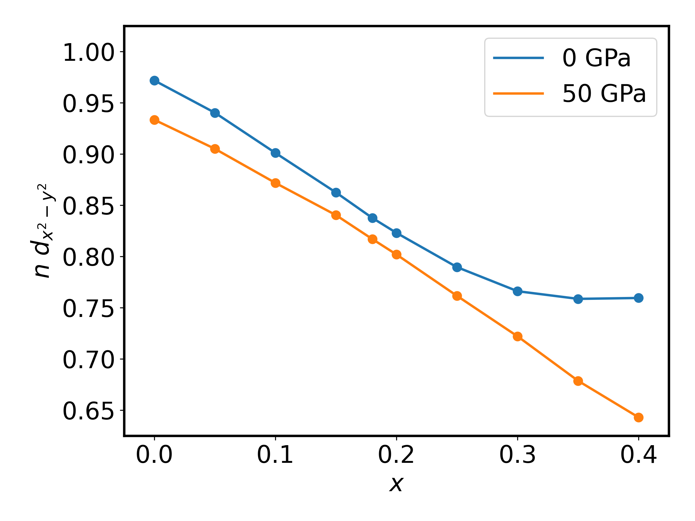
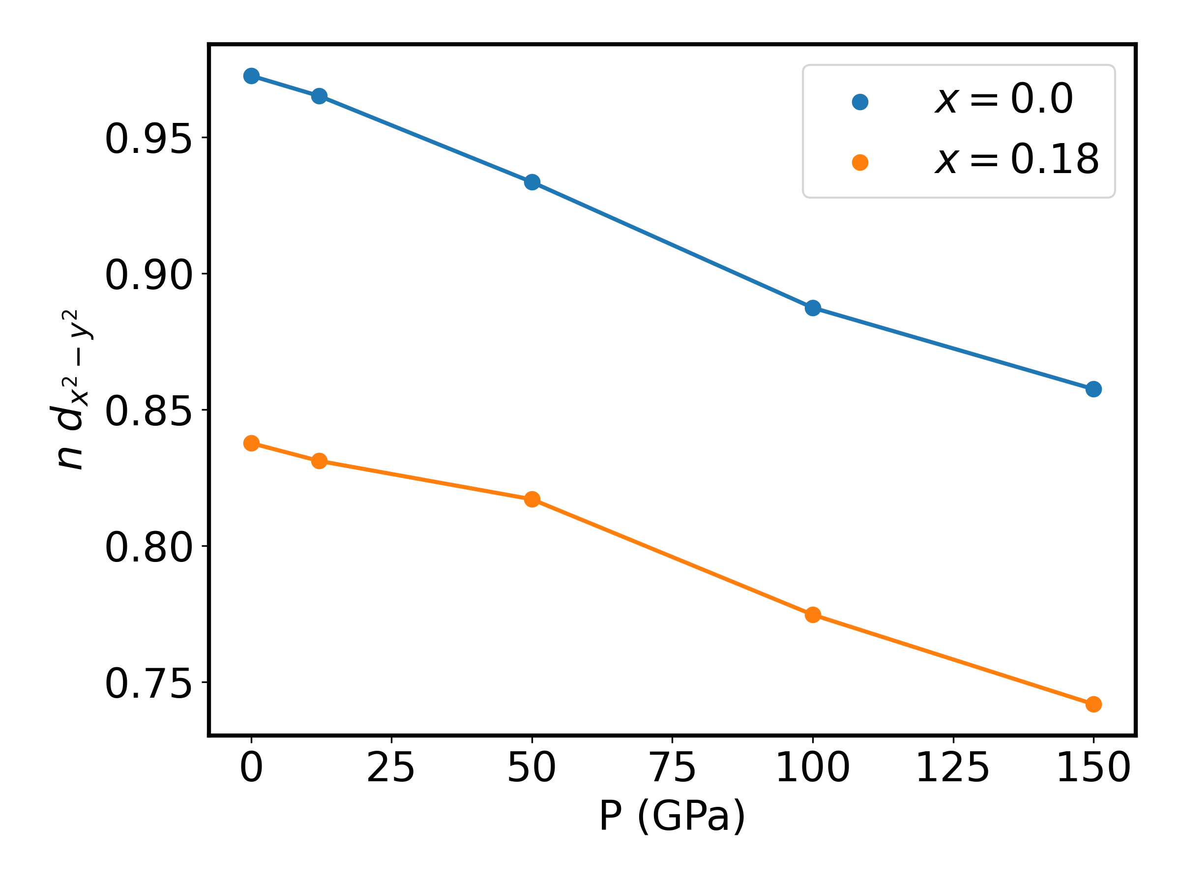
Figure S6: Left panel: Effective filling $n_{d_{x^{2}-y^{2}}}$ of the Ni $d_{x^{2}-y^{2}}$band as a function of Sr doping $x$, calculated in DMFT for the 10-band model. The results for 0 and 50 GPa are indicated as blue and orange lines, respectively. Right panel: $n_{d_{x^{2}-y^{2}}}$ of the Ni $d_{x^{2}-y^{2}}$band as a function of pressure at fixed doping $x=0.00$ (blue curve) and $x=0.18$ (orange curve). The hole doping of the main text is $\delta=1-n_{d_{x^{2}-y^{2}}}$.

In addition to Fig. 2 of the main text, we show in Fig S7 the DMFT bandstructure of the parent compound, PrNiO$-2$, at further pressures, visualizing the evolution with pressure. This is supplemented by the Fermi surface displayed in Fig. S8 for the same pressure and doping $x=0$. Note that at 150 GPa the electron pocket around $\Gamma$ becomes so large that it touches the Ni $d_{x^{2}-y^{2}}$band. At pressures higher than this point, the description of the correlated system in terms of 1 correlated orbital plus decoupled pockets likely needs to be refined.

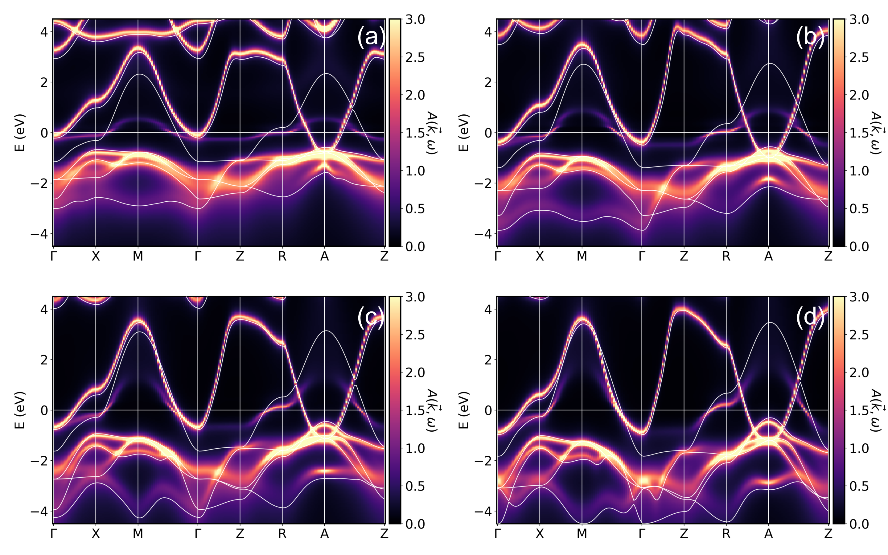
Figure S7: Evolution of the spectral function $A(\textbf{k},\omega)$ of PrNiO₂ along a high-symmetry path in reciprocal space for the 10-bands DMFT calculations. (a), (b), (c), and (d) correspond to calculations at 12, 50, 100, and 150 GPa, respectively. The spectral function $A(\textbf{k},\omega)$ is shown as a color scale. The DFT bands interpolated from Wannier functions are shown as white lines.

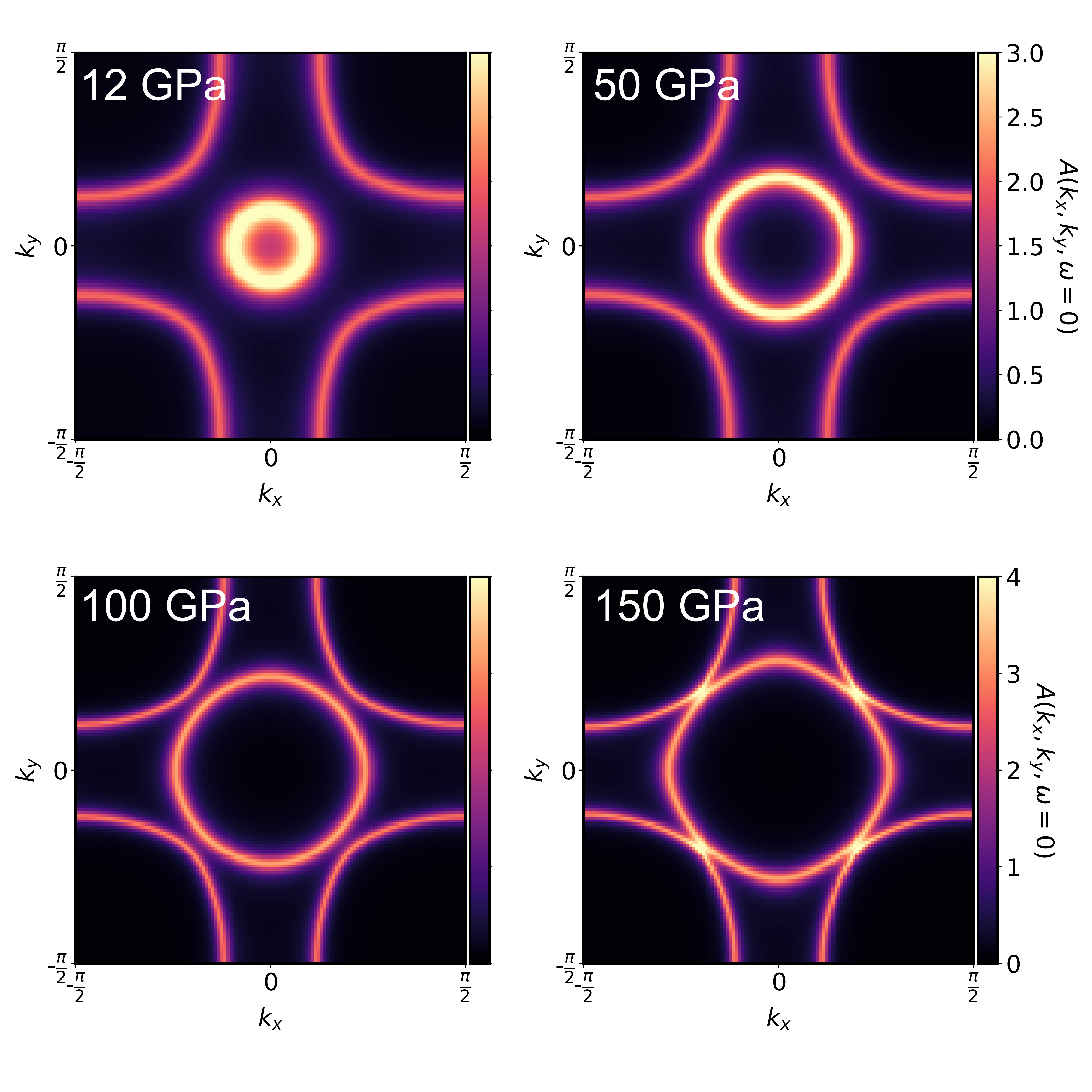
Figure S8: Evolution of the spectral function $A(\textbf{k},\omega)$ of PrNiO₂ along the Fermi surface at $k_{z}=0$ for the undoped PrNiO₂ as a function of pressure.

In Fig. 3 of the main text, we showed the evolution of the 1-band DFT+DMFT spectrum of the parent compound ($x=0$) as a function of pressure. This corresponds to path (c) in Fig. 1 and 4 of main text. Here, we also show the evolution with doping at 0 GPa [Fig. S9, path (a)] and 50 GPa [Fig. S10, path (b)]; as well as the pressure dependence for doping $x=0.18$ [Fig. S11, path (d)].

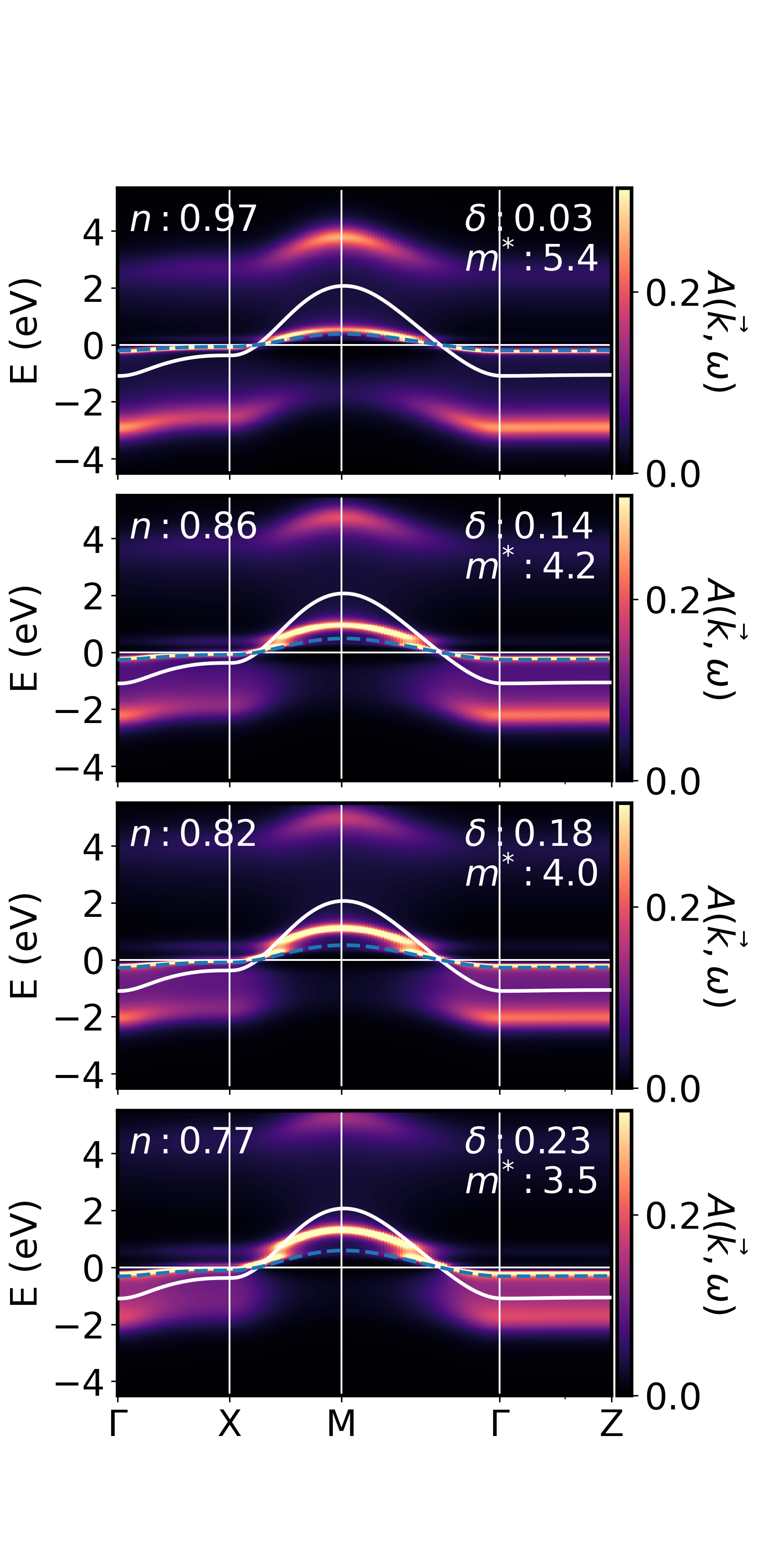
Figure S9: Spectral function computed from the local self-energy at fixed pressure P = 0 GPa as a function of doping $x$, from 0.0 to 0.30, at $\beta=80t$. The spectral function $A(\textbf{k},\omega)$ is shown as a color gradient.

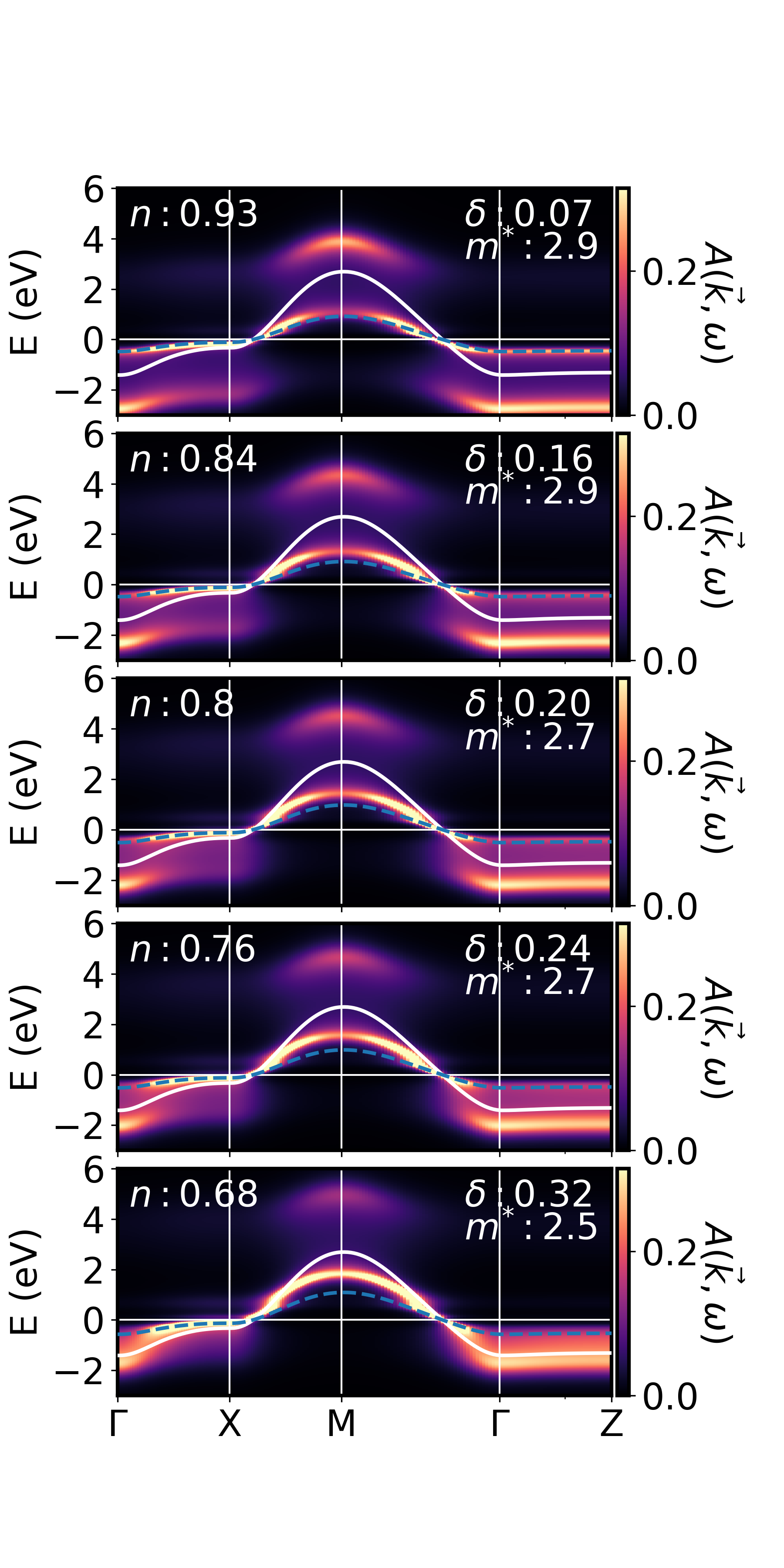
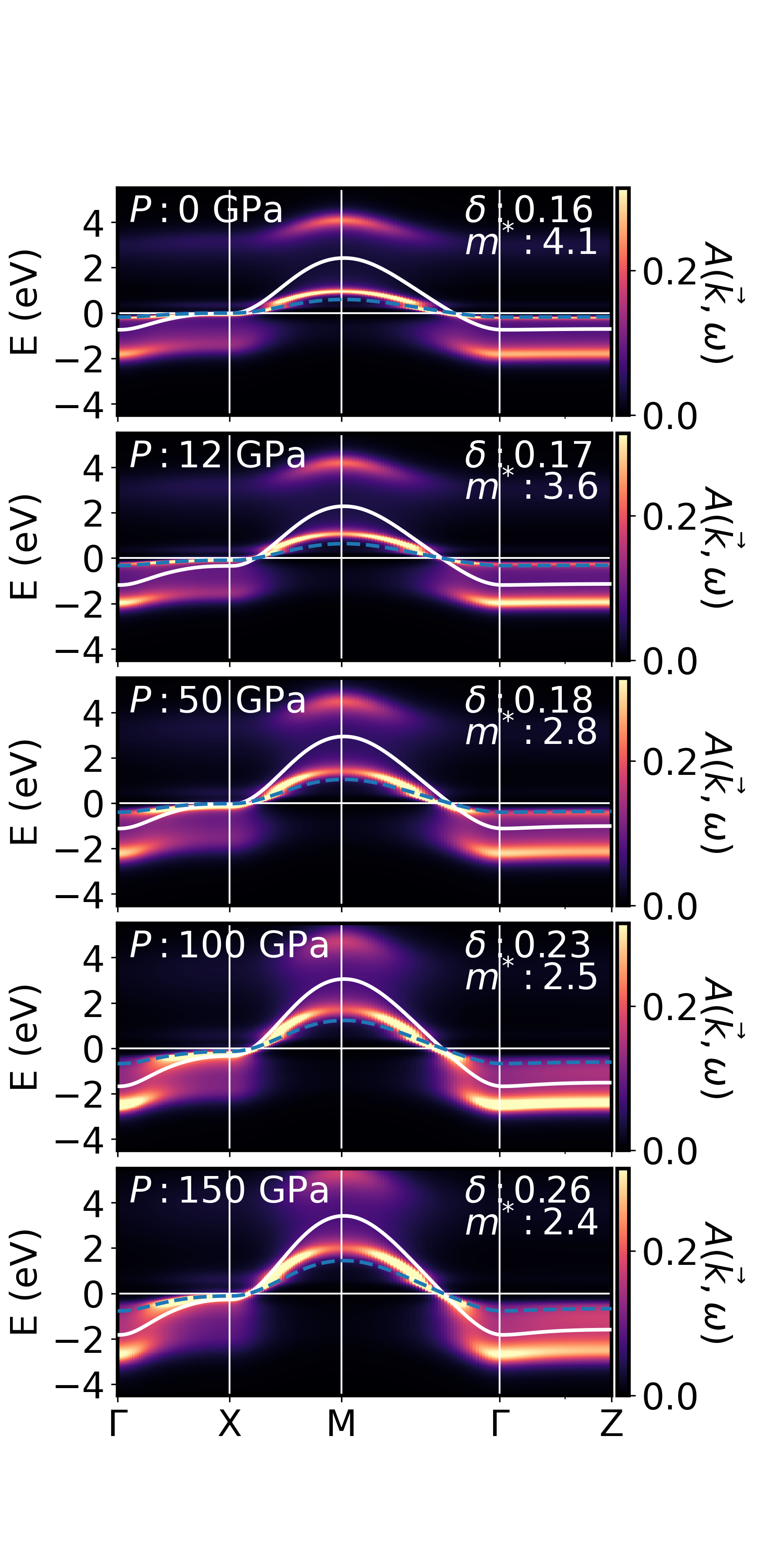
Figure S10: Spectral function computed from the local self-energy at fixed pressure P = 50 GPa as a function of doping $x$, from 0.0 to 0.30, at $\beta=80t$. The spectral function $A(\textbf{k},\omega)$ is shown as a color gradient.

Figure S11: Spectral function computed from the local self-energy at fixed doping $x=0.18$ and as a function of pressure, from 0 to 150, at $\beta=80t$. The spectral function $A(\textbf{k},\omega)$ is shown as a color gradient.

VII.2 Superconductivity in D$\Gamma$A

In this section we present some additional comparisons of the superconducting phase diagram. First, in Fig. S12, we compare the superconducting dome of Sr_xPr_1-xNiO₂ to that of Sr_xNd_1-xNiO₂ calculated in [2]. Both phase diagrams are in good agreement and the deviations, including the slightly lower $T_{\text{c}}$in Sr_xPr_1-xNiO₂ can be explained by the different $A$ cation (Pr instead of Nd).

Second in Fig. S14, we plot the change of $T_{\text{c}}$ as a function of pressure together with the change of $t$. This comparison clearly reveals that the difference between the parent compound (left) and 18% Sr-doping (right) originates from the parent compound moving to optimal doping at 100 GPa, whereas the doped sample moves from optimal doping to overdoped with pressure.

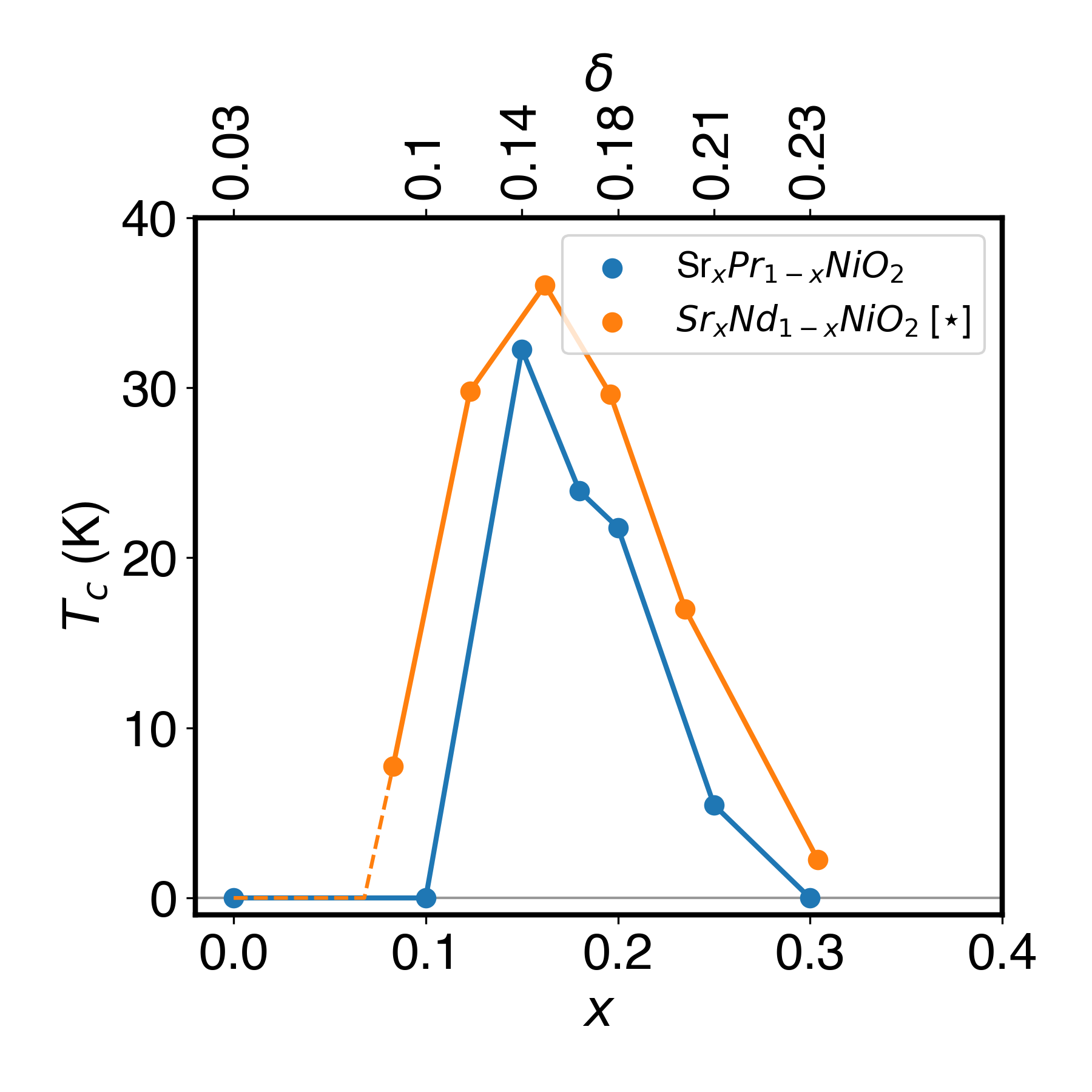
Figure S12: Comparison of the superconducting dome at 0 GPa calculated for Sr_xPr_1-xNiO₂ (our work) and for Sr_xNd_1-xNiO₂ (Ref. [2]).

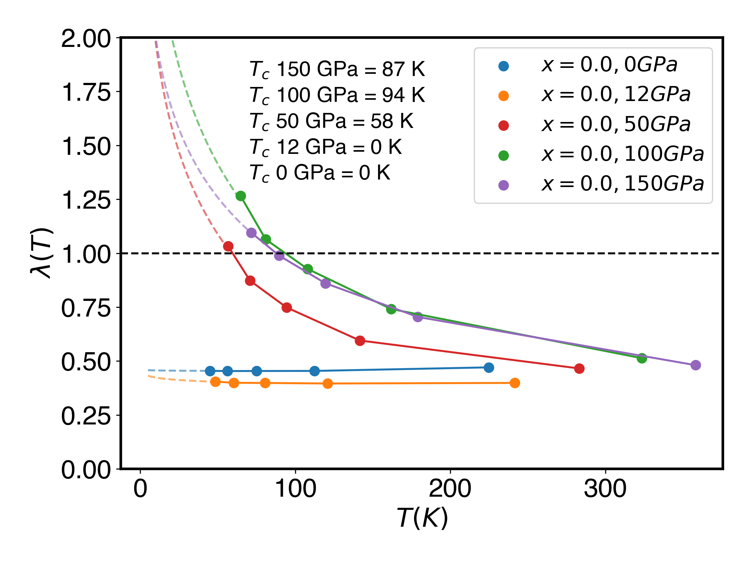
Figure S13: Leading superconducting eigenvalue $\lambda$ as a function of temperature at $x=0$ and as a function of pressure. The critical temperature is selected as the value at which the curve (or its extrapolation) crosses the $\lambda=1$ line.

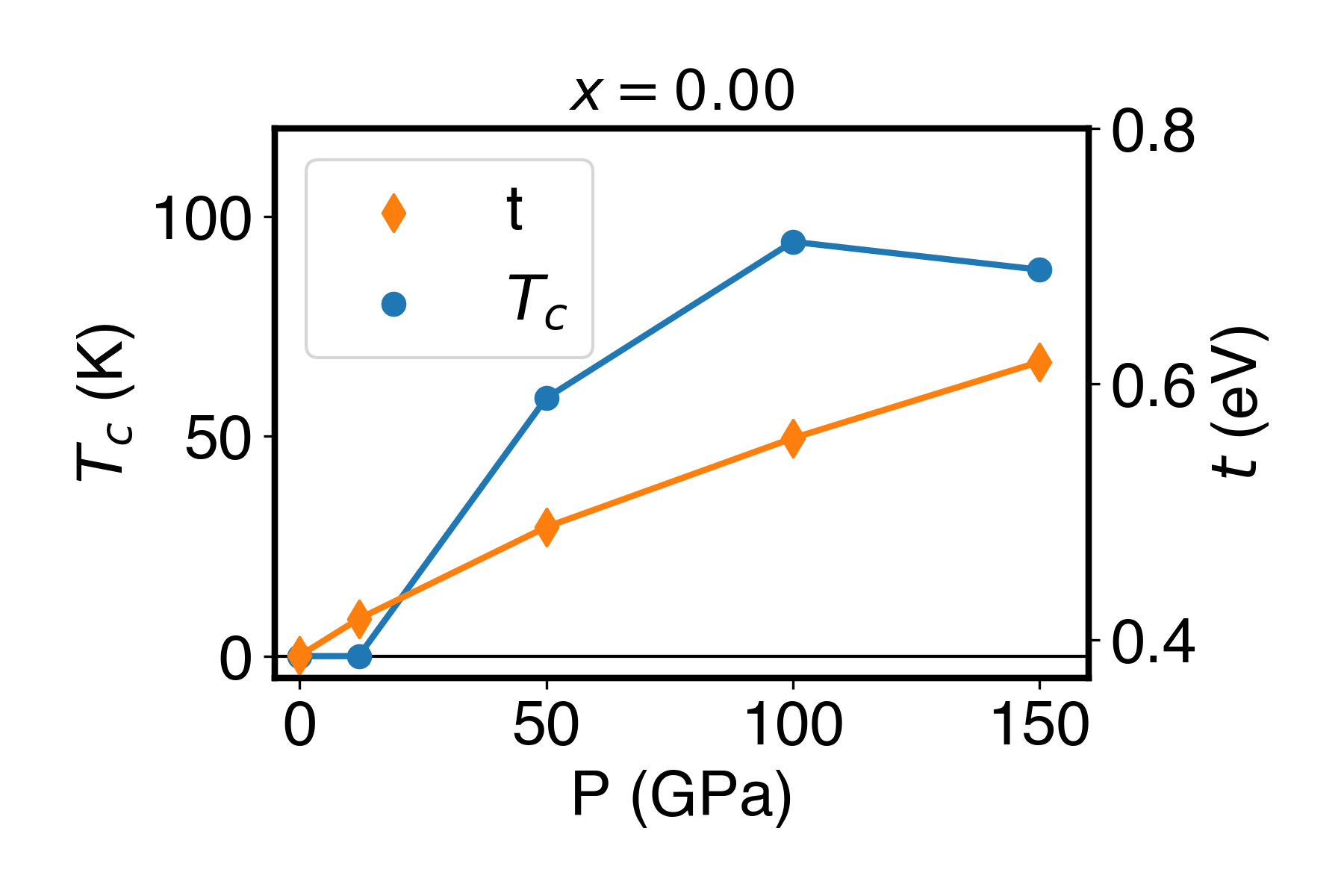
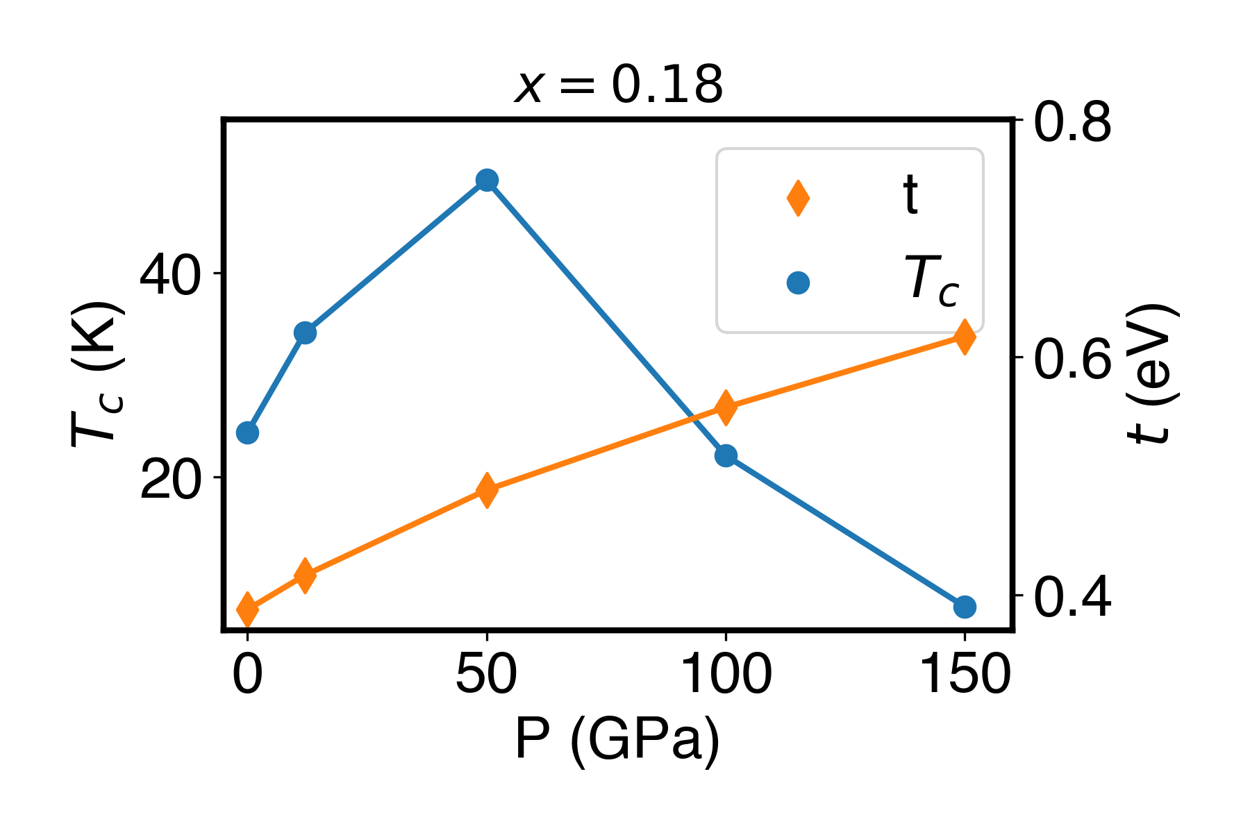
Figure S14: Trend of the superconducting $T_{\text{c}}$ as a function of pressure, compared with the first-nearest-neighbor hopping $t$.

VII.3 Tests of the Virtual Crystal Approximation

The Virtual Crystal Approximation should be approached carefully, especially when it is employed to interpolate between two atoms that are not adjacent on the periodic table.

We performed extensive checks of the quality of the Virtual Crystal Approximation (VCA) to simulate an average mixture of praseodymium (Pr) and strontium (Sr). In the following, we list the tests and their result, and briefly discuss their implication.

Vergard’s Law

The first simple test is to check that Vergard’s Law is respected [34], i.e. that the lattice parameter of the intermediate alloy is a weighted mean of the two isolate compounds. In Fig. S15 we report a comparison between the lattice parameter of a Pr-Sr mixture in a face-centered cubic structure at different concentrations, obtained with the VCA and in a 2$\times$2$\times$2 supercell. We note that not only the law is respected, but even the small deviation from the linear behavior are matched by the calculations in the supercell, i.e. they are a physical deviation, rather than an artifact of the VCA.

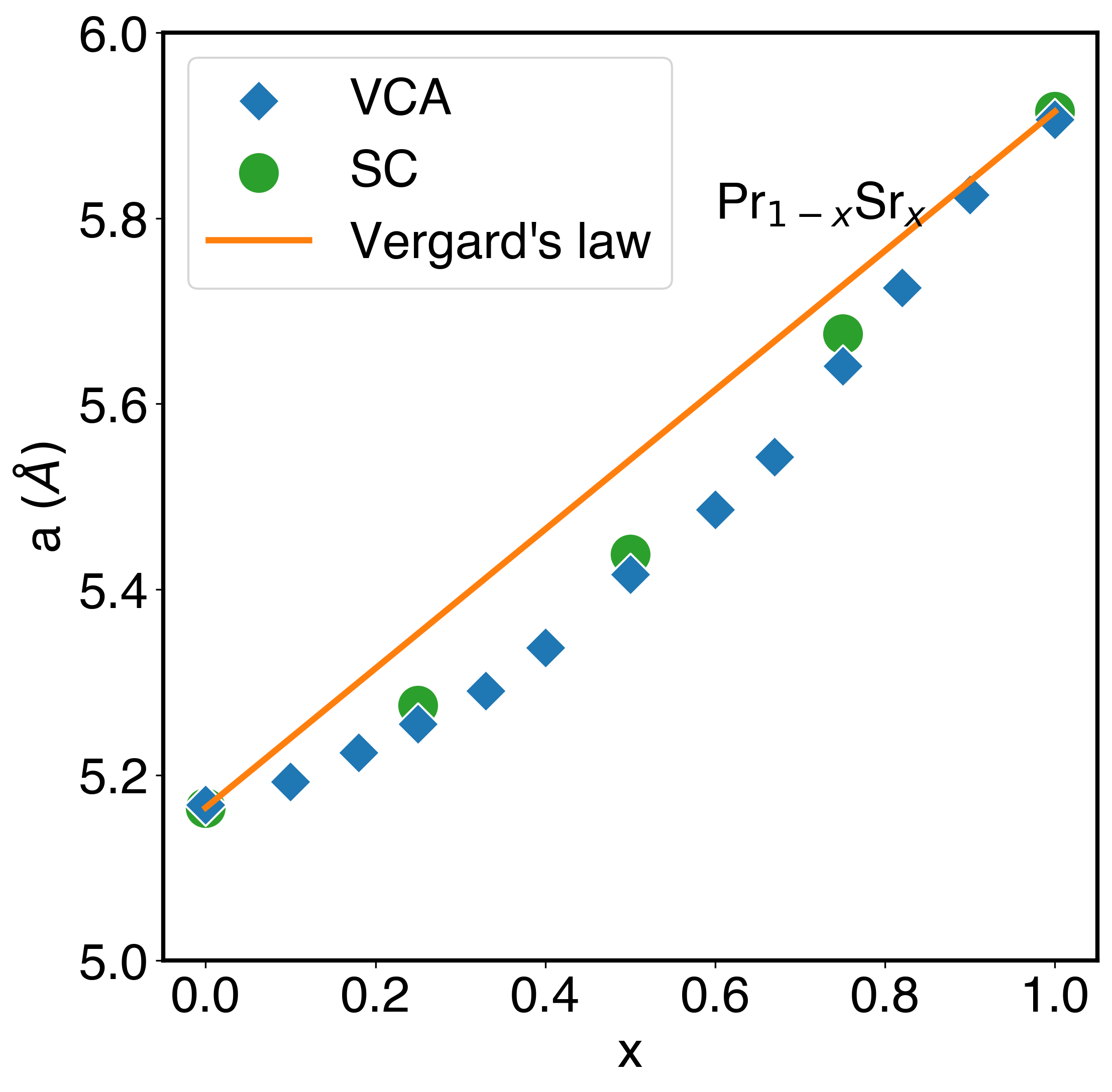
Figure S15: Vergard’s Law for a Pr-Sr alloy in the face-centered cubic phase. Blue diamonds, green circles, and the orange line indicate the result obtained using the VCA, a 2$\times$2$\times$2 supercell, and the ideal law, respectively.

$c$ axis of Pr_0.75Sr_0.25NiO₂

We checked the consistency of the VCA in the specific environment of interest, i.e. the Pr_1-xSr_xNiO₂ nickelate. A doping of $x=0.25$ can be simulated in a relatively small 2$\times$2$\times$2 supercell, and its effect on the structural properties compared with the VCA result.

In Fig. S4 we show the change in enthalpy of Pr_0.75Sr_0.25NiO₂ as a function of the $c$ axis using the VCA and in five different supercell configurations. The equilibrium $c$ value thus obtained is identical for all the cases considered, and close to the experimental value [9], and deviations are only seen away from equilibrium.

Electronic structure

The last test involves a direct comparison of the electronic band structure between the VCA case and the five inequivalent supercells at $x=0.25$. We employed the relaxed structures describe in the previous paragraph, but we note that their lattice parameters are identical within DFT accuracy. In Fig. S16 we show the electronic band structure for the VCA and the five different supercells. Also in this case the two results are in excellent agreement, with only a few minute differences due to the symmetry breaking induced by Sr in the supercell, which splits a few bands.

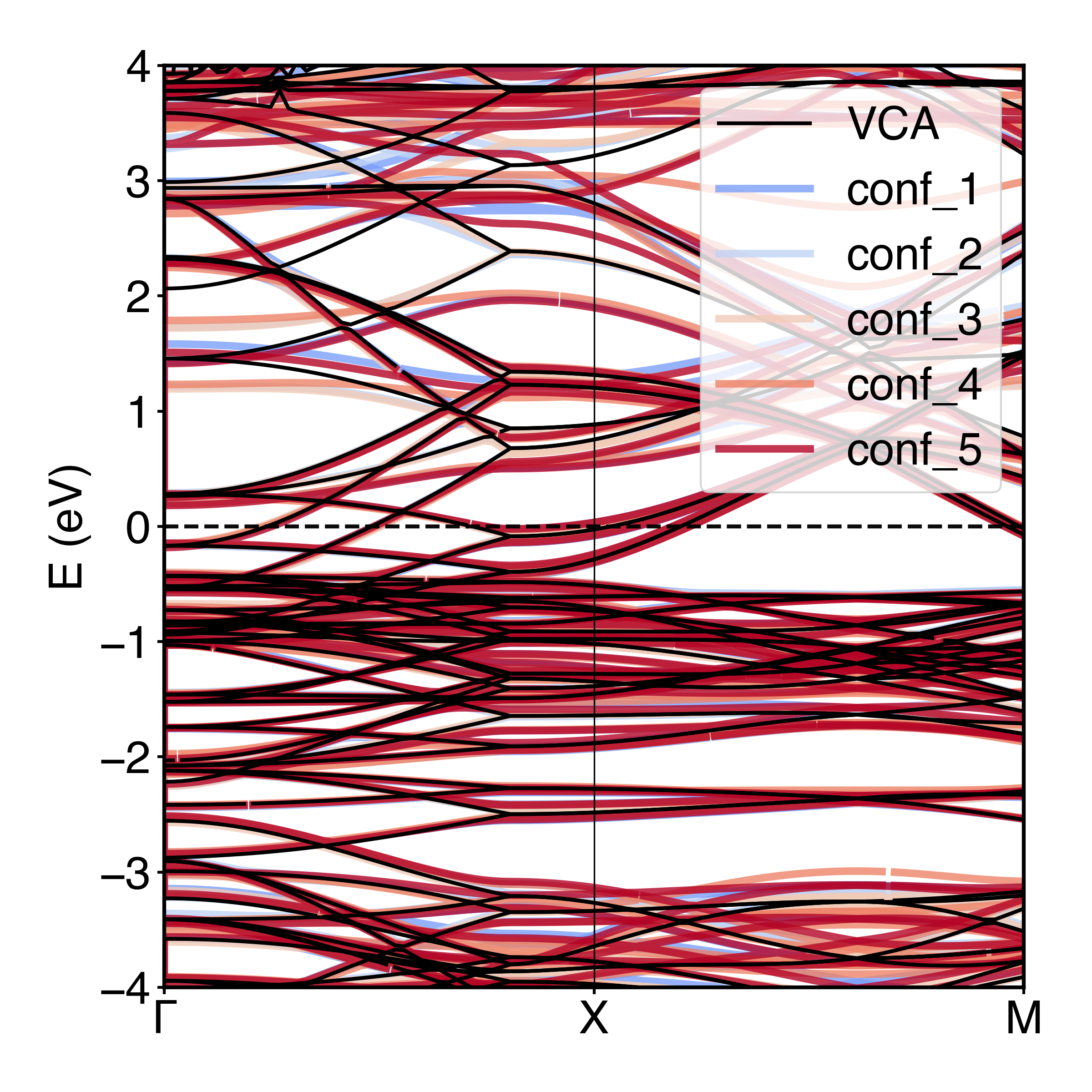
Figure S16: Electronic band structure for Pr_0.75Sr_0.25NiO₂ using the VCA and in five different supercells. The VCA value is shown as a black line, and the results for the supercells are shown as colored lines.

References

- Bednorz and Müller [1986] J. G. Bednorz and K. A. Müller, Zeitschrift für Physik B Condensed Matter 64, 189 (1986).
- Li et al. [2019] D. Li, K. Lee, B. Y. Wang, M. Osada, S. Crossley, H. R. Lee, Y. Cui, Y. Hikita, and H. Y. Hwang, Nature 572, 624 (2019).
- Osada et al. [2020a] M. Osada, B. Y. Wang, K. Lee, D. Li, and H. Y. Hwang, Phys. Rev. Materials 4, 121801 (2020a).
- Zeng et al. [2020] S. Zeng, C. S. Tang, X. Yin, C. Li, M. Li, Z. Huang, J. Hu, W. Liu, G. J. Omar, H. Jani, Z. S. Lim, K. Han, D. Wan, P. Yang, S. J. Pennycook, A. T. S. Wee, and A. Ariando, Phys. Rev. Lett. 125, 147003 (2020).
- Zeng et al. [2022] S. Zeng, C. Li, L. E. Chow, Y. Cao, Z. Zhang, C. S. Tang, X. Yin, Z. S. Lim, J. Hu, P. Yang, et al., Science advances 8, eabl9927 (2022).
- Osada et al. [2021] M. Osada, B. Y. Wang, B. H. Goodge, S. P. Harvey, K. Lee, D. Li, L. F. Kourkoutis, and H. Y. Hwang, Advanced Materials n/a, 2104083 (2021).
- Pan et al. [2021a] G. A. Pan, D. F. Segedin, H. LaBollita, Q. Song, E. M. Nica, B. H. Goodge, A. T. Pierce, S. Doyle, S. Novakov, D. C. Carrizales, et al., Nature Materials 10.1038/s41563-021-01142-9 (2021a).
- Anisimov et al. [1999] V. I. Anisimov, D. Bukhvalov, and T. M. Rice, Phys. Rev. B 59, 7901 (1999).
- Chow and Ariando [2022] L. E. Chow and A. Ariando, Fron. Phys. 10, 834658 (2022).
- [10] Q. N. Meier, J. B. de Vaulx, F. Bernardini, A. S. Botana, X. Blase, V. Olevano, and A. Cano, arXiv:2309.05486 .
- [11] S. D. Cataldo, P. Worm, L. Si, and K. Held, arXiv:2304.03599 .
- Nomura et al. [2019] Y. Nomura, M. Hirayama, T. Tadano, Y. Yoshimoto, K. Nakamura, , and R. Arita, Physical Review B 100, 205138 (2019).
- Held et al. [2022] K. Held, L. Si, P. Worm, O. Janson, R. Arita, Z. Zhong, J. M. Tomczak, and M. Kitatani, Frontiers in Physics 9, 10.3389/fphy.2021.810394 (2022).
- Botana and Norman [2020] A. S. Botana and M. R. Norman, Phys. Rev. X 10, 011024 (2020).
- Wang et al. [2020] Z. Wang, G.-M. Zhang, Y.-f. Yang, and F.-C. Zhang, Phys. Rev. B 102, 220501 (2020).
- Sakakibara et al. [2020] H. Sakakibara, H. Usui, K. Suzuki, T. Kotani, H. Aoki, and K. Kuroki, Phys. Rev. Lett. 125, 077003 (2020).
- Wu et al. [2020] X. Wu, D. Di Sante, T. Schwemmer, W. Hanke, H. Y. Hwang, S. Raghu, and R. Thomale, Phys. Rev. B 101, 060504 (2020).
- Jiang et al. [2019] P. Jiang, L. Si, Z. Liao, and Z. Zhong, Phys. Rev. B 100, 201106 (2019).
- Hirayama et al. [2020] M. Hirayama, T. Tadano, Y. Nomura, and R. Arita, Phys. Rev. B 101, 075107 (2020).
- Kitatani et al. [2020] M. Kitatani, L. Si, O. Janson, R. Arita, Z. Zhong, and K. Held, npj Quantum Materials 5, 59 (2020).
- Karp et al. [2020] J. Karp, A. S. Botana, M. R. Norman, H. Park, M. Zingl, and A. Millis, Phys. Rev. X 10, 021061 (2020).
- Pascut et al. [2023] G. Pascut, L. Cosovanu, K. Haule, and K. F. Quader, Commun. Phys. 6, 45 (2023).
- Adhikary et al. [2020] P. Adhikary, S. Bandyopadhyay, T. Das, I. Dasgupta, and T. Saha-Dasgupta, Phys. Rev. B 102, 100501 (2020).
- Lechermann [2020] F. Lechermann, Phys. Rev. B 101, 081110 (2020).
- Petocchi et al. [2020] F. Petocchi, V. Christiansson, F. Nilsson, F. Aryasetiawan, and P. Werner, Phys. Rev. X 10, 041047 (2020).
- Qin et al. [2023] C. Qin, M. Jiang, and L. Si, Phys. Rev. B 108, 155147 (2023).
- Lee et al. [2022] K. Lee, B. Y. Wang, M. Osada, B. H. Goodge, T. C. Wang, Y. Lee, S. Harvey, W. J. Kim, Y. Yu, C. Murthy, et al., arXiv preprint arXiv:2203.02580 (2022).
- Worm et al. [2022] P. Worm, L. Si, M. Kitatani, R. Arita, J. M. Tomczak, and K. Held, Phys. Rev. Materials 6, L091801 (2022).
- Pan et al. [2021b] G. A. Pan, D. F. Segedin, H. LaBollita, Q. Song, E. M. Nica, B. H. Goodge, A. T. Pierce, S. Doyle, S. Novakov, D. C. Carrizales, A. T. N’Diaye, P. Shafer, H. Paik, J. T. Heron, J. A. Mason, A. Yacoby, L. F. Kourkoutis, O. Erten, C. M. Brooks, A. S. Botana, and J. A. Mundy, Nature Materials 10.1038/s41563-021-01142-9 (2021b).
- Kitatani et al. [2023] M. Kitatani, L. Si, P. Worm, J. M. Tomczak, R. Arita, and K. Held, Phys. Rev. Lett. 130, 166002 (2023).
- Wang et al. [2022] N. N. Wang, M. W. Yang, K. Y. Chen, Z. Yang, H. Zhang, Z. H. Zhu, Y. Uwatoko, X. L. Dong, K. J. Jin, J. P. Sun, and J. G. Cheng, Nature Communications 13, 4367 (2022).
- Christiansson et al. [2023] V. Christiansson, F. Petocchi, and P. Werner, Phys. Rev. B 107, 045144 (2023).
- [33] H. Sun, X. Huo, M. Hu, J. Li, Z. Liu, Y. Han, L. Tang, Z. Mao, P. Yang, B. Wang, J. Cheng, D.-X. Yao, Z. G.-M., and M. Wang, Nature 621, 493.
- Sakakibara et al. [2023] H. Sakakibara, M. Ochi, H. Nagata, Y. Ueki, H. Sakurai, R. Matsumoto, K. Terashima, K. Hirose, H. Ohta, M. Kato, Y. Takano, and K. Kuroki, arXiv:2309.09462 10.48550/arXiv.2309.09462 (2023).
- Osada et al. [2020b] M. Osada, B. Y. Wang, B. H. Goodge, K. Lee, H. Yoon, K. Sakuma, D. Li, M. Miura, L. F. Kourkoutis, and H. Y. Hwang, Nano Letters 20, 5735 (2020b).
- Tomczak et al. [2009] J. M. Tomczak, T. Miyake, R. Sakuma, and F. Aryasetiawan, Phys. Rev. B 79, 235133 (2009).
- [37] Supplemental information regarding details of DFT, DMFT and DA calculations and further results are available at XXX.
- Kitatani et al. [2022] M. Kitatani, R. Arita, T. Schäfer, and K. Held, Journal of Physics: Materials 5, 034005 (2022).
- Si et al. [2020] L. Si, W. Xiao, J. Kaufmann, J. M. Tomczak, Y. Lu, Z. Zhong, and K. Held, Phys. Rev. Lett. 124, 166402 (2020).
- Rohringer et al. [2018] G. Rohringer, A. Katanin, T. Schäfer, A. Hausoel, K. Held, and A. Toschi, github.com/ladderDGA (2018), github.com/ladderDGA .
- Wang et al. [2022] N. Wang, M. Yang, K. Chen, Z. Yang, H. Zhang, Z. Zhu, Y. Uwatoko, X. Dong, K. Jin, J. Sun, et al., Nature Comm. , 4367 (2022).
- Savchenko et al. [1986] V. Savchenko, L. Ivashkevich, and V. Meleshko, Inorganic Materials 21, 1499 (1986).
- Ismailzade et al. [1971] I. Ismailzade, G. Smolenskii, V. Nesterenko, and F. Agaev, physica status solidi (a) 5, 83 (1971).
- Shishido et al. [1995] T. Shishido, S. Nojima, M. Tanaka, H. Horiuchi, and T. Fukuda, Journal of alloys and compounds 227, 175 (1995).
- [45] Additional data related to this publication, including input/output files and raw data for both DFT and DMFT calculations is available at DOI:10.48436/9xych-d8n28.
- Kresse and Furthmüller [1996] G. Kresse and J. Furthmüller, Phys. Rev. B 54, 11169 (1996).
- Kresse and Furthmüller [1999] G. Kresse and J. Furthmüller, Phys. Rev. B 59, 1758 (1999).
- Perdew et al. [1996] J. P. Perdew, K. Burke, and M. Ernzerhof, Phys. Rev. Lett. 77, 3865 (1996).
- Perdew et al. [2008] J. P. Perdew, A. Ruzsinszky, G. I. Csonka, O. A. Vydrov, G. E. Scuseria, L. A. Constantin, X. Zhou, and K. Burke, Phys. Rev. Lett. 100, 136406 (2008).
- Mostofi et al. [2008] A. A. Mostofi, J. R. Yates, Y.-S. Lee, I. Souza, D. Vanderbilt, and N. Marzari, Computer Physics Communications 178, 685 (2008).
- Miyake and Aryasetiawan [2008] T. Miyake and F. Aryasetiawan, Phys. Rev. B 77, 085122 (2008).
- Miyake et al. [2009] T. Miyake, F. Aryasetiawan, and M. Imada, Phys. Rev. B 80, 155134 (2009).
- Methfessel et al. [2000] M. Methfessel, M. van Schilfgaarde, and R. Casali, in Electronic Structure and Physical Properties of Solids: The Uses of the LMTO Method, Lecture Notes in Physics. H. Dreysse, ed. 535, 114 (2000).
- Wallerberger et al. [2019] M. Wallerberger, A. Hausoel, P. Gunacker, A. Kowalski, N. Parragh, F. Goth, K. Held, and G. Sangiovanni, Comp. Phys. Comm. 235, 388 (2019).
- [55] https://nomad-lab.eu/prod/v1/gui/user/uploads/upload/id/fRI7D7sdTQO0f6H_bPPgCg.
- Scheidgen et al. [2023] M. Scheidgen, L. Himanen, A. Ladines, D. Sikter, M. Nakhaee, A. Fekete, T. Chang, A. Golparvar, J. Márquez, S. Brockhauser, S. Brückner, L. Ghiringhelli, F. Dietrich, D. Lehmberg, T. Denell, A. Albino, H. Näsström, S. Shabih, F. Dobener, M. Kühbach, R. Mozumder, J. Rudzinski, N. Daelman, J. Pizarro, M. Kuban, C. Salazar, P. Ondraka, H.-J. Bungartz, and C. Draxl, Journal of Open Source Software 8, 5388 (2023).

References

- [1] Additional data related to this publication, including input/output files and raw data for both DFT and DMFT calculations is available at DOI:10.48436/9xych-d8n28.
- Kitatani et al. [2020] M. Kitatani, L. Si, O. Janson, R. Arita, Z. Zhong, and K. Held, npj Quantum Materials 5, 59 (2020).
- Kresse and Furthmüller [1996] G. Kresse and J. Furthmüller, Phys. Rev. B 54, 11169 (1996).
- Perdew et al. [2008] J. P. Perdew, A. Ruzsinszky, G. I. Csonka, O. A. Vydrov, G. E. Scuseria, L. A. Constantin, X. Zhou, and K. Burke, Phys. Rev. Lett. 100, 136406 (2008).
- Kresse and Furthmüller [1999] G. Kresse and J. Furthmüller, Phys. Rev. B 59, 1758 (1999).
- Bellaiche and Vanderbilt [2000] L. Bellaiche and D. Vanderbilt, Phys. Rev. B 61, 7877 (2000).
- Christiansson et al. [2023] V. Christiansson, F. Petocchi, and P. Werner, Phys. Rev. B 107, 045144 (2023).
- Li et al. [2019] D. Li, K. Lee, B. Y. Wang, M. Osada, S. Crossley, H. R. Lee, Y. Cui, Y. Hikita, and H. Y. Hwang, Nature 572, 624 (2019).
- Osada et al. [2020] M. Osada, B. Y. Wang, B. H. Goodge, K. Lee, H. Yoon, K. Sakuma, D. Li, M. Miura, L. F. Kourkoutis, and H. Y. Hwang, Nano Letters 20, 5735 (2020).
- Zeng et al. [2020] S. Zeng, C. S. Tang, X. Yin, C. Li, M. Li, Z. Huang, J. Hu, W. Liu, G. J. Omar, H. Jani, Z. S. Lim, K. Han, D. Wan, P. Yang, S. J. Pennycook, A. T. S. Wee, and A. Ariando, Phys. Rev. Lett. 125, 147003 (2020).
- Lee et al. [2020] K. Lee, B. H. Goodge, D. Li, M. Osada, B. Y. Wang, Y. Cui, L. F. Kourkoutis, and H. Y. Hwang, APL Materials 8, 041107 (2020).
- Osada et al. [2021] M. Osada, B. Y. Wang, B. H. Goodge, S. P. Harvey, K. Lee, D. Li, L. F. Kourkoutis, and H. Y. Hwang, Advanced Materials n/a, 2104083 (2021).
- Wang et al. [2022] N. N. Wang, M. W. Yang, K. Y. Chen, Z. Yang, H. Zhang, Z. H. Zhu, Y. Uwatoko, X. L. Dong, K. J. Jin, J. P. Sun, and J. G. Cheng, Nature Communications 13, 4367 (2022).
- Ikeda et al. [2014] A. Ikeda, T. Manabe, and M. Naito, Physica C 506, 83 (2014).
- Lee et al. [2022] K. Lee, B. Y. Wang, M. Osada, B. H. Goodge, T. C. Wang, Y. Lee, S. Harvey, W. J. Kim, Y. Yu, C. Murthy, et al., arXiv preprint arXiv:2203.02580 (2022).
- Zeng et al. [2022] S. Zeng, C. Li, L. E. Chow, Y. Cao, Z. Zhang, C. S. Tang, X. Yin, Z. S. Lim, J. Hu, P. Yang, et al., Science advances 8, eabl9927 (2022).
- Murnaghan [1944] F. D. Murnaghan, Proceedings of the National Academy of Sciences of the United States of America 30, 244 (1944), http://www.pnas.org/content/30/9/244.full.pdf+html .
- Mostofi et al. [2008] A. A. Mostofi, J. R. Yates, Y.-S. Lee, I. Souza, D. Vanderbilt, and N. Marzari, Computer Physics Communications 178, 685 (2008).
- Miyake and Aryasetiawan [2008] T. Miyake and F. Aryasetiawan, Phys. Rev. B 77, 085122 (2008).
- Miyake et al. [2009] T. Miyake, F. Aryasetiawan, and M. Imada, Phys. Rev. B 80, 155134 (2009).
- Methfessel et al. [2000] M. Methfessel, M. van Schilfgaarde, and R. Casali, in Electronic Structure and Physical Properties of Solids: The Uses of the LMTO Method, Lecture Notes in Physics. H. Dreysse, ed. 535, 114 (2000).
- Tomczak et al. [2009] J. M. Tomczak, T. Miyake, R. Sakuma, and F. Aryasetiawan, Phys. Rev. B 79, 235133 (2009).
- Ivashko et al. [2019] O. Ivashko, M. Horio, W. Wan, N. Christensen, D. McNally, E. Paris, Y. Tseng, N. E. Shaik, H. M. Rønnow, H. I. Wei, C. Adamo, C. Lichtensteiger, M. Gibert, M. R. Beasley, K. M. Shen, J. M. Tomczak, T. Schmitt, and J. Chang, Nature Comm. 10, 786 (2019).
- Si et al. [2020] L. Si, W. Xiao, J. Kaufmann, J. M. Tomczak, Y. Lu, Z. Zhong, and K. Held, Phys. Rev. Lett. 124, 166402 (2020).
- Georges et al. [1996] A. Georges, G. Kotliar, W. Krauth, and M. J. Rozenberg, Rev. Mod. Phys. 68, 13 (1996).
- Held [2007] K. Held, Advances in physics 56, 829 (2007).
- Parragh et al. [2012] N. Parragh, A. Toschi, K. Held, and G. Sangiovanni, Phys. Rev. B 86, 155158 (2012).
- Wallerberger et al. [2019] M. Wallerberger, A. Hausoel, P. Gunacker, A. Kowalski, N. Parragh, F. Goth, K. Held, and G. Sangiovanni, Comp. Phys. Comm. 235, 388 (2019).
- Kitatani et al. [2022] M. Kitatani, R. Arita, T. Schäfer, and K. Held, Journal of Physics: Materials 5, 034005 (2022).
- Toschi et al. [2007] A. Toschi, A. A. Katanin, and K. Held, Phys Rev. B 75, 045118 (2007).
- Katanin et al. [2009] A. A. Katanin, A. Toschi, and K. Held, Phys. Rev. B 80, 075104 (2009).
- Rohringer et al. [2018] G. Rohringer, A. Katanin, T. Schäfer, A. Hausoel, K. Held, and A. Toschi, github.com/ladderDGA (2018), github.com/ladderDGA .
- Kitatani et al. [2019] M. Kitatani, T. Schäfer, H. Aoki, and K. Held, Phys. Rev. B 99, 041115 (2019).
- Denton and Ashcroft [2004] A. R. Denton and N. W. Ashcroft, Physical Review A 43, 3161 (2004).