Greedy PIG: Adaptive Integrated Gradients

Abstract

Deep learning has become the standard approach for most machine learning tasks. While its impact is undeniable, interpreting the predictions of deep learning models from a human perspective remains a challenge. In contrast to model training, model interpretability is harder to quantify and pose as an explicit optimization problem. Inspired by the AUC softmax information curve (AUC SIC) metric for evaluating feature attribution methods, we propose a unified discrete optimization framework for feature attribution and feature selection based on subset selection. This leads to a natural adaptive generalization of the path integrated gradients (PIG) method for feature attribution, which we call Greedy PIG. We demonstrate the success of Greedy PIG on a wide variety of tasks, including image feature attribution, graph compression/explanation, and post-hoc feature selection on tabular data. Our results show that introducing adaptivity is a powerful and versatile method for making attribution methods more powerful.

1 Introduction

Deep learning sets state-of-the-art on a wide variety of machine learning tasks, including image recognition, natural language understanding, large-scale recommender systems, and generative models (Graves et al., 2013; He et al., 2016; Krizhevsky et al., 2017; Bubeck et al., 2023). Deep learning models, however, are often opaque and hard to interpret. There is no native procedure for explaining model decisions to humans, and explainability is essential when models make decisions that directly influence people’s lives, e.g., in healthcare, epidemiology, legal, and education (Ahmad et al., 2018; Wiens and Shenoy, 2018; Chen et al., 2021a; Abebe et al., 2022; Liu et al., 2023).

We are interested in two routines: (i) feature attribution and (ii) feature selection. Given an input example, feature attribution techniques offer an explanation of the model’s decision by assigning an attribution score to each input feature. These scores can then be directly rendered in the input space, e.g., as a heatmap highlighting visual saliency (Sundararajan et al., 2017), offering an explanation of model decisions that is human-interpretable. On the other hand, feature selection methods find the set of most-informative features for a machine learning model across many examples to optimize its prediction quality. While the goal of both feature attribution and feature selection is to find the most impactful features, they are inherently different tasks with a disjoint set of approaches and literature. Concretely, feature attribution considers one example per invocation, while feature selection considers an entire dataset. For literature surveys, see (Zhang et al., 2021) for feature attribution and interpretability see and (Li et al., 2017) for feature selection.

Our main contributions are as follows:

• We consider the problem of feature attribution from first principles and, inspired by evaluation metrics in the literature (Kapishnikov et al., 2019), we propose a new formulation of feature attribution as an explicit subset selection problem.

• Using this subset selection formulation, we ascribe the main shortcomings of the path integrated gradient (PIG) algorithms to their limited ability to handle feature correlations. This motivates us to introduce adaptivity to these algorithms, which is a natural way to account for correlations, leading to a new algorithm that we call Greedy PIG.

• We leverage the generality of the subset selection formulation to propose different objectives for feature attribution based on model loss that can better capture the model’s behavior, as well as a unification between feature attribution and feature selection formulations.

• We evaluate the performance of Greedy PIG on a variety of experimental tasks, including feature attribution, graph neural network (GNN) compression, and post-hoc feature selection. Our results show that adaptivity is a powerful ingredient for improving the quality of deep learning model interpretability methods.

2 Preliminaries

2.1 Path integrated gradients (PIG)

Let $f(\cdot;\bm{\mathit{\theta}})$ be a pre-trained neural network with parameters $\bm{\mathit{\theta}}$. Our work assumes that $f$ is pre-trained and therefore, we often omit $\bm{\mathit{\theta}}$ for brevity. Suppose $\bm{\mathit{x}}\in\mathbb{R}^{n}$ is an input example. The path integrated gradients (PIG) method of Sundararajan et al. (2017) attributes the decision of $f$ given $\bm{\mathit{x}}$, by considering a line path from the “baseline” example $\bm{\mathit{x}}^{(0)}$ to $\bm{\mathit{x}}$:

$$\gamma:[0,1]\rightarrow\mathbb{R}^{n}\ \ \ \ \ \textrm{with}\ \ \ \ \ \gamma(t;\bm{\mathit{x}}^{(0)},\bm{\mathit{x}})=\bm{\mathit{x}}^{(0)}+t(\bm{\mathit{x}}-\bm{\mathit{x}}^{(0)})\ \ \ \ \ \textrm{for}\ \ \ \ t\in[0,1].$$ (1)

Then, the top features $i\in[n]$ maximizing the following (weighted) integral are chosen:

$$\operatorname*{arg\,sort}_{i\in[n]}\ \ \ \left[\ \ \ (\bm{\mathit{x}}_{[i]}-\bm{\mathit{x}}^{(0)}_{[i]})\int_{0}^{1}\frac{\partial}{\partial\bm{\mathit{x}}_{[i]}}f(\gamma(t))dt\ \ \ \right].$$ (2)

Our work addresses a weakness of PIG, which is that it is a one-shot algorithm. Specifically, an invocation to PIG computes (in-parallel) Eq. 1 and chooses (at-once) the indices $\subseteq[n]$ maximizing Eq. 2.

2.2 Subset selection

Subset selection is a family of discrete optimization problems, where the goal is to select a subset $S\subseteq[n]:=\{1,2,\dots,n\}$ that maximizes a set function $G:2^{[n]}\rightarrow\mathbb{R}$ subject to a cardinality constraint $k$:

$$S^{*}=\operatorname*{arg\,max}_{S\subseteq[n],|S|\leq k}G(S).$$ (3)

Prominent examples of subset selection in machine learning include data summarization (Kleindessner et al., 2019), feature selection (Cai et al., 2018; Elenberg et al., 2018; Bateni et al., 2019; Chen et al., 2021b; Yasuda et al., 2023), and submodular optimization (Krause and Golovin, 2014; Mirrokni and Zadimoghaddam, 2015; Fahrbach et al., 2019a, b).

Throughout our work, we let $\mathbf{1}$ denote $n$-dimensional all-one vector, $\mathbf{1}_{S}\in\{0,1\}^{n}$ be the indicator vector of $S$, and let $\bm{\mathit{x}}_{S}=\mathbf{1}_{S}\odot\bm{\mathit{x}}\in\mathbb{R}^{n}$ where $\odot$ denotes Hadamard product.

3 Our method

3.1 Motivation: Discrete optimization for feature attribution and selection

The general subset selection framework (§2.2) allows recovering several tasks. For (i) feature attribution, the softmax information curve (SIC) of Kapishnikov et al. (2019) can be recovered from (Eq. 3) by setting $G(S)$ to the softmax output of a target class (see Eq. 4). For (ii) feature selection, we can set $G(S)$ to maximum log likelihood achievable by a model trained on a subset of features $S$. Finally, if one sets $G(S)$ to be the maximum model output perturbation achieved by only changing the values of features in $S$, one recovers a task of finding counterfactual explanations.

The generality of framework (§2.2) encourages us to pose the tasks (i) and (ii) as instances. Consequently, we inherit algorithms and intuitions from the subset selection and submodular optimization literature. The area of submodular optimization has a vast literature with different theoretical analyses and algorithms based on the specific properties of the set function. For example, for maximization of weakly submodular functions, it is known that the greedy subset selection algorithm achieves a constant approximation ratio. In general, determining the right realistic assumptions on the set function is a major open problem in the area. As such, it is not yet clear which of these assumptions are realistic for each use case. We believe this is a very important question for future work.

3.2 Instantiations

Multi-class attribution.

Suppose that classifier $f$ is the softmax output of a multi-class neural network, then the softmax information curve of Kapishnikov et al. (2019) can be written in (§4.1; Eq. 3) as:

$$G^{\textsc{AttributionSoftmax}}(S)=f_{c^{*}}(\bm{\mathit{x}}_{S})\,,\ \ \ \ \textrm{with}\ \ \ \ c^{*}=\mathop{\arg\max}_{j}f_{j}(\bm{\mathit{x}}).$$ (4)

Maximizing $S$ in Eq. 4 chooses feature subset $S$ that maintains the model’s decision, as compared to the fully-observed example $\bm{\mathit{x}}$. Crucially, however, the top class $c^{*}$ doesn’t tell the whole story, since the input might be ambiguous or the classifier might be uncertain. It is then natural that one would want to capture the behavior of $f$ on all classes, rather than just the top one. A natural alternative is to re-use the objective ($\ell$) that the model was trained with, and incorporate it into a subset selection problem. Specifically, we define the set function:

$$G^{\textsc{AttributionKL}}(S)=\ell(f(\bm{\mathit{x}}),f(\bm{\mathit{x}}_{S}))=f(\bm{\mathit{x}})\log f(\bm{\mathit{x}}_{S})\,,$$ (5)

where, for classification, $\ell$ is the log-likelihood. This quantifies the similarity of probability distribution $f(\bm{\mathit{x}}_{S})$, i.e., considering a subset of features, with the distribution $f(\bm{\mathit{x}})$, i.e., considering all features. Maximizing $G(S)$ under a cardinality constraint is then equivalent to seeking a small number of features that capture the multiclass behavior of the model on a fixed input example.

Feature selection.

Unlike feature attribution, outputting attributions for a single example, in feature selection, the goal is to select a global set of features for all dataset examples, that maximize the predictive capability of the model. Feature selection can be formulated by defining

$$G^{\textsc{FeatSelect}}(S)=\max_{\bm{\mathit{\theta}}}\ell(\bm{\mathit{y}},f(\bm{\mathit{X}}_{S};\bm{\mathit{\theta}}))\,,$$ (6)

i.e., the maximum log likelihood obtainable by training the model $f$ on the whole dataset $\bm{\mathit{X}}$, given only the features in $S$. Such formulation of feature selection as subset selection has been studied extensively, e.g., (Liberty and Sviridenko, 2017; Elenberg et al., 2018; Bateni et al., 2019; Chen et al., 2021b; Yasuda et al., 2023; Axiotis and Yasuda, 2023). To avoid re-training $f$, we consider a simpler problem of post-hoc feature selection, with $G^{\textsc{FeatSelectPH}}(S)=\ell(\bm{\mathit{y}},f(\bm{\mathit{X}}_{S};\bm{\mathit{\theta}}))$ where the model parameters $\bm{\mathit{\theta}}$ are pre-trained on all features.We leave further investigation of (6) to future work. The post-hoc formulation has the advantage of making the objective differentiable, and thus directly amenable to gradient-based approaches, while also not requiring access to the training process of $f$, which is seen as a black box. This can be particularly useful for applications with limited resources or engineering constraints that discourage running or modifying the training pipeline. As we will show in §5.3, high quality feature selection can be performed even in this restricted setting.

3.3 Continuous extension

To make the problem (Eq. 3) amenable to continuous optimization methods, we rely on a continuous extension $g:[0,1]^{n}\rightarrow\mathbb{R}$ with $G(S):=g(\mathbf{1}_{S})$. The extension can be derived by replacing the invocation of $f$ on $\bm{\mathit{x}}_{S}$ or $\bm{\mathit{X}}_{S}$ in Eq. 4–6 by an invocation on a path, similar to Eq. 1, but with domain equal to the $n$-hypercube:

$$g:[0,1]^{n}\rightarrow\mathbb{R}^{n}\ \ \ \ \ \textrm{with}\ \ \ \ \ g(\mathbf{s};\bm{\mathit{x}}^{(0)},\bm{\mathit{x}})=\bm{\mathit{x}}^{(0)}+\mathbf{s}\odot(\bm{\mathit{x}}-\bm{\mathit{x}}^{(0)})\ \ \ \ \ \textrm{for}\ \ \ \ \mathbf{s}\in[0,1]^{n}.$$ (7)

This makes it easy to adapt feature attribution methods from the literature to our framework and is a lightweight assumption since loss functions in deep learning are continuous by definition. In particular, the integrated gradients algorithm of Sundararajan et al. (2017) can simply be stated as computing the vector of feature scores given by $\int_{t=0}^{1}\nabla g(t\mathbf{1})dt$.

3.4 Greedy path integrated gradients (Greedy PIG)

We now move to identify and improve the weaknesses of the integrated gradients algorithm. In contrast to previous works that focus on reducing the amount of “noise” perceived by humans in the attribution result, we identify a different weakness of PIG—it is sensitive to feature correlations. In §4.1, we show that even in simple linear regression settings, PIG exhibits pathologies such as outputting attribution scores that are negative, or whose ordering can be manipulated via feature replication. This leads us to introduce adaptivity to the algorithm. We are motivated by the greedy algorithm for subset selection, which is known to provably tackle submodular optimization problems, even when there are strong correlations between features.

Why Greedy captures correlations.

A remarkable property of the greedy algorithm is that its adaptivity property can automatically deal with correlations. Consider a set function $G$ and three elements $i,j,k$. Suppose that greedy initially selects element $i$. Then, it will recurse on the residual set function $G^{\prime}(S)=G(S\cup\{i\})$. Thus, in the next phases, correlations between $i$ and the remaining elements are eliminated, since $i$ is fixed (selected). In other words, since greedy conditions on the already selected variables, this eliminates their correlations with the rest of the unselected variables.

Greedy PIG.

Inspired by the adaptivity complexity of submodular maximization (Balkanski and Singer, 2018), where it has been shown that $\Omega(\log n/\log\log n)$ adaptive rounds of evaluating $G$ are needed to achieve provably-better solution quality than one-shot algorithms (such as integrated gradients), we propose a generalization of integrated gradients with multiple rounds. We call this algorithm Greedy PIG since it greedily selects the top-attribution features computed by integrated gradients in each round, i.e. the set of $S\subseteq[n]$ maximizing the $\arg\,\textrm{sort}$ of Eq. 2, and hardcodes their corresponding entries in $\mathbf{s}$ to 1.

3.5 The greedy PIG algorithm

Our idea is to iteratively compute the top features as attributed by integrated gradients, and select these features by always including them in future runs of integrated gradients (and only varying the rest of the variables along the integration path). We present this algorithm in detail in Algorithm 1.

Algorithm 1 Greedy PIG (path integrated gradients)

1:Input: access to a gradient oracle for $g:[0,1]^{n}\rightarrow\mathbb{R}$

2:Input: number of rounds $R$, number of selections per round $z$

3:Initialize $S\leftarrow\varnothing$ $\triangleright$ Selected set of features

4:Initialize $\bm{\mathit{a}}\leftarrow\mathbf{0}$ $\triangleright$ Vector of attributions

5:for $r=1$ to $R$ do

6:     Set $\hat{\bm{\mathit{a}}}\leftarrow\int_{t=0}^{1}\nabla_{\bar{S}}g(\mathbf{1}_{S}+t\mathbf{1}_{\bar{S}})dt$

7:     Set $\hat{S}\leftarrow\mathrm{top}_{z}(\hat{\bm{\mathit{a}}})$ $\triangleright$ Top-$z$ largest entries of $\hat{\bm{\mathit{a}}}$

8:     Update $\bm{\mathit{a}}\leftarrow\bm{\mathit{a}}+\hat{\bm{\mathit{a}}}_{\hat{S}}$

9:     Update $S\leftarrow S\cup\hat{S}$ return $\bm{\mathit{a}},S$

In practice, Greedy PIG can be implemented by repeated invocations of PIG (Eq. 1&2). The impact of $g$ (Eq. 7) can be realized by iteratively updating:

$$\hat{S}\leftarrow\textrm{top indices of Eq.~{}\ref{eq:pig_argsort} with \ \ }\gamma(.;\bm{\mathit{x}}^{(j+1)},\bm{\mathit{x}})\textrm{ \ \ with \ \ }\ \ \bm{\mathit{x}}^{(j+1)}\leftarrow\bm{\mathit{x}}_{\hat{S}}+\bm{\mathit{x}}^{(j)}_{\bar{\hat{S}}}$$ (8)

Specifically, Greedy PIG is related to a continuous version of Greedy. In the continuous setting, selecting an element $i$ is equivalent to fixing the $i$-th element of the baseline to its final value. The $i$-th element now does not vary and its correlations with the remaining elements are eliminated. At a high level, our approach has similarities to (Kapishnikov et al., 2021), which adaptively computes the trajectory of the PIG path based on gradient computations.

Similar to previous work, the integral in Algorithm 1 on 6 can be estimated by discretizing it into a number of steps. A simpler approach that we found to be competitive and more frugal is to approximate the integral by a single gradient $\nabla_{\bar{S}}g(\mathbf{1}_{S})$, which we call the Sequential Gradient (SG) algorithm. It should be noted that, in contrast to integrated gradients, Algorithm 1 empirically does not return negative attributions.

4 Analysis

4.1 Attribution as subset selection

The integrated gradients method is widely used because of its simplicity and usefulness. Since its inception, it was known to satisfy two axioms that Sundararajan et al. (2017) called sensitivity and implementation invariance, as well as the convenient property that the sum of attributions is equal to the function value. However, there is still no deep theoretical understanding of when this method (or any attribution method, for that matter) succeeds or fails, or even how success is defined.

Previous works have studied a variety of failure cases. In fact, it is well-observed that the attributions on image datasets are often “grainy,” a property deemed undesirable from a human standpoint (although as stated before, it is not necessarily bad as long as the attributions are highly predictive of the model’s output). In addition, there will almost always exist some negative attribution scores, whose magnitude can be even higher than that of positive attribution scores. There have been efforts to mitigate these effects for computer vision tasks, most notably by ascribing them to noise (Smilkov et al., 2017; Adebayo et al., 2018), region grouping (Ancona et al., 2017; Kapishnikov et al., 2019), or ascribing them to the magnitude of the gradient (Kapishnikov et al., 2021).

In this work, we take a different approach and start from the basic question:

What are attribution scores supposed to compute?

An important step towards answering this question was done in (Kapishnikov et al., 2019), which defined the softmax information curve (SIC) for image classification. In short, the idea is that if we only keep $k$ features with the top attributions and drop the rest of the features, the softmax output of the predicted class should be as large as possible. This is because then, the model prediction can be distilled down to a small number of features.

Based on the above intuition, we define the problem in a more general form:

Definition 4.1 (Attribution as subset selection).

Given a set function $G:2^{[n]}\rightarrow\mathbb{R}_{>0}$, a value $k\in[n]$, and a permutation $\bm{\mathit{r}}=(r_{1},r_{2},\dots,r_{n})$ of $[n]$, the attribution quality of $\bm{\mathit{r}}$ at level $k$ is defined as

$$\frac{G(\{r_{1},r_{2},\dots,r_{k}\})}{\max_{S\subseteq[n]:|S|=k}G(S)}.$$

We define the attribution quality of $\bm{\mathit{r}}$ (without reference to $k$) as the area under the curve defined by the points $(k,G(\{r_{1},r_{2},\dots,r_{k}\})$ for all $k\in[n]$.

The key advantage of this approach is that we are able to pose attribution as an explicit optimization problem, and hence we are able to compare, evaluate, and analyze the quality of attribution methods. In addition, the formulation in Definition 4.1 gives us flexibility in picking the objective $G$ to be maximized. In fact, in §5.1 we propose setting $G$ to be the log likelihood (i.e., negative cross entropy loss) instead of the top softmax score. In §5.3, we will see how this formulation allows us to tie attribution together with feature selection.

Note.

As Definition 4.1 shows, we are interested in the problem of attributing predictions to a small number of features. For example, when faced with redundant features, we wish to pinpoint only a small number of them. This does not capture applications in which the goal is to find the attribution for all features, where the goal would be to assign equal attribution score to all redundant features.

4.2 Correlations and adaptivity

Given the problem formulation in Definition 4.1, we are ready to study the strengths and weaknesses of attribution methods. First, it is important to define the notion of marginal gain, which is a central notion in subset selection problems.

Definition 4.2 (Marginal gain).

Given a set function $G:2^{[n]}\rightarrow\mathbb{R}_{\geq 0}$, the marginal gain of the $i$-th element at $S\subseteq[n]$ is defined by $G(S\cup\{i\})-G(S)$. When $S$ is omitted, we simply define the marginal gain as $G(\{i\})-G(\varnothing)$.

Marginal gains are important because they are closely related to the well-studied greedy algorithm for subset selection (Nemhauser et al., 1978), and are crucial for its analysis. Therefore, a natural question arises: Are the outputs of attribution methods correlated with the marginal gains?

For this, let us assume that the set function $G$ is induced by a continuous relaxation $g:[0,1]^{n}\rightarrow\mathbb{R}$. We show that the integrated gradient attributions approximate the marginal gains up to an additive term that depends on the second-order behavior of $g$, and corresponds to the amount of correlation between variables. In fact, when the variables are uncorrelated, integrated gradient attributions are equal to the marginal gains.

Lemma 4.3 (PIG vs marginal gain).

Let $H(\bm{\mathit{w}})$ be the Hessian of a twice continuously differentiable function $g:[0,1]^{n}\rightarrow\mathbb{R}$ at $\bm{\mathit{w}}$. Then, for all $i\in[n]$,

$$\left|\int_{t=0}^{1}\nabla_{i}g(t\mathbf{1})dt-(g(\mathbf{1}_{i})-g(\mathbf{0}))\right|\leq\frac{1}{2}\max_{\bm{\mathit{w}}\in[0,1]^{n},i\in[n]}\left|\sum_{j\neq i}H_{ij}(\bm{\mathit{w}})\right|\,,$$

where $\mathbf{1}_{i}$ is the $i$-th standard basis vector of $\mathbb{R}^{n}$.

Lemma 4.3 tells us that the quality of how well the integrated gradient attribution scores approximate the marginal gains is strongly connected to correlations between input variables. Indeed, if these correlations are too strong, the attributions can diverge in magnitude and sign, even in simple settings. This motivates combining integrated gradients with adaptivity (e.g. the Greedy algorithm), since adaptivity naturally takes correlations into account. The Greedy PIG algorithm, which we will define in §3.5, is a natural combination of integrated gradients and Greedy.

We now look at a more concrete failure case of integrated gradients in Lemma 4.4, that can arise because of feature redundancy, and how adaptivity can help overcome this issue.

Lemma 4.4 (Feature redundancy).

Consider a continuous set function $g:[0,1]^{n}\rightarrow\mathbb{R}$ and $t$ redundant features numbered $1,2,\dots,t$, or in other words for any $\bm{\mathit{w}}\in[0,1]^{n}$ we have $g((w_{1},\dots,w_{n}))=h((\max\{w_{1},\dots,w_{t}\},w_{t+1},\dots,w_{n}))$ for some $h:[0,1]^{n-t+1}\rightarrow\mathbb{R}$. Then, the integrated gradients algorithm with a baseline of $\mathbf{0}$ will assign equal attribution score to features $1$ through $t$.

It follows from Lemma 4.4 that it is possible to replicate the top-attributed feature multiple times such that the top attributions are all placed on redundant copies of the same feature, therefore missing features $t+1$ through $n$. This behavior arises because integrated gradients is a one-shot algorithm, but it can be remedied by introducing adaptivity. Specifically, if we select one of the features with top attributions, e.g., feature $1$ and then re-run integrated gradients with an updated baseline $(1,0,\dots,0)^{\top}$, then the new attribution scores of the redundant features $2,\dots,t$ will be $0$. Therefore, the remaining $k-1$ top attributions will be placed on the remaining features $t+1,\dots,n$.

5 Experimental Evaluation

In this section, we evaluate the effect of the adaptivity introduced by Greedy PIG. A comparison with all attribution methods is out of scope, mainly because our proposed modification can be easily adapted to other algorithms (e.g., SmoothGrad), and so, even though we provide comparisons with different popular methods, we mostly concentrate on integrated gradients. We defer an evaluation of adaptive generalizations of other one-shot algorithms to future work.

5.1 Feature attribution for image recognition

Experimental setup.

We use the MobileNetV2 neural network (Sandler et al., 2018) pretrained on ImageNet, and compare different feature attribution methods on individual Imagenet examples. We use the all-zero baseline for integrated gradients, which, because of the data preprocessing pipeline of MobileNetV2, corresponds to an all-gray image. To ensure that our results hold across models, we present additional results on ResNet50 in the appendix.

Top-class attribution.

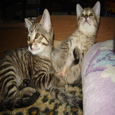
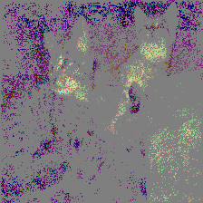
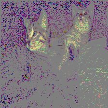
(a) Top $15000$ features attributed by integrated gradients (left) vs. GreedyPIG (right). The softmax output for true class “tabby” after pruning unselected features is $3\cdot 10^{-5}$ for integrated gradients vs. $0.9973$ for GreedyPIG.

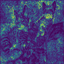
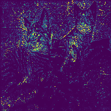
(b) Heatmap of feature attributions by integrated gradients (left) vs. GreedyPIG (right).

Figure 7: Illustration of attribution algorithms on an example from Imagenet labeled “tabby” (left column). Integrated gradients (IG) (middle) ran for $2000$ steps, while GreedyPIG (right) ran for $100$ rounds each with $20$ steps. Both IG and GreedyPIG maximized softmax objective.

Kapishnikov et al. (2019) introduced the softmax information curve for image classification, which plots the output softmax probability of the target class using only the top attributions, as a function of the compressed image size. Since we are interested in a general method, we instead plot the output softmax as a function of the number of top selected features. To perform attribution based on our framework, we let $c^{*}$ be the class output by the model $f(\bm{\mathit{x}};\bm{\mathit{\theta}})$ on input $\bm{\mathit{x}}$ and with parameters $\bm{\mathit{\theta}}$, and then define $g^{\mathrm{top1}}(\mathbf{s}):=f_{c^{*}}(\bm{\mathit{x}}\odot\mathbf{s};\bm{\mathit{\theta}}))$, where $\mathbf{s}\in[0,1]^{n}$ and $\odot$ denotes the Hadamard product. In other words, $g^{\mathrm{top1}}$ gives the softmax output of the (fixed) class predicted by the model, after re-weighting input features by $\mathbf{s}$. We can now run gradient-based attribution algorithms on $g$. The results can be found in Figure 1 and Figure 7.

Loss attribution.

Even though the top class attribution methodology can explain what are the most important features that influence the model’s top predicted class, it might fail to capture other aspects of the model’s behavior. For example, if the model has low certainty in its prediction, the softmax output of the top class will be low. In fact, in such cases the attribution method can select a number of features that give a much more confident output. However, it can instead be useful to capture the outputs of all classes, and not just the top one. More generally, we can use arbitrary loss functions to attribute certain aspects of the model’s behavior to the features.

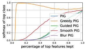
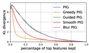
Algorithm	softmax AUC $(\uparrow)$	KL divergence AUC $(\downarrow)$
Integrated Gradients (Sundararajan et al., 2017)	$0.2639$	$2.0812$
Smooth PIG (Smilkov et al., 2017)	$0.4433$	$1.1366$
Blur PIG (Xu et al., 2020)	$0.1903$	$2.0812$
Guided PIG (Kapishnikov et al., 2021)	$0.2623$	$2.0644$
Greedy PIG	${\bf 0.8486}$	${\bf 0.6655}$

Figure 1: Evaluating the attribution performance across $1466$ examples randomly drawn from Imagenet. The Softmax Information Curve (SIC) plots the softmax output of the top class as a function of the number of features kept (there are $224\times 224\times 3$ features total for these RGB images). The Loss Information Curve (LIC) similarly plots the KL divergence from the output probabilities on the features kept, to the output probabilities when all features are kept. To compute these results, we run integrated gradients and guided integrated gradients with $2000$ steps and Greedy PIG with $100$ rounds, $20$ steps each. Then, for each algorithm and number of features kept, we compute and plot the median across all examples, as in Kapishnikov et al. (2019). Left: The Softmax Information Curve (higher is better). Right: The Loss Information Curve (lower is better).

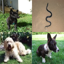
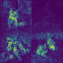
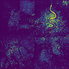
(a) Top 15000 attributions for class “sea snake”. Left: input, Middle: integrated gradients, Right: Greedy PIG.

Algorithm	pointing accuracy $(\uparrow)$
Integrated Gradients (Sundararajan et al., 2017)	$0.66$
Greedy PIG	${\bf 0.83}$

(b) Pointing accuracy aggregated over $25$ $2x2$ grids generated from examples that had the highest prediction confidence from $1500$ examples randomly drawn from the validation set of ImageNet.

Figure 2: Results from the pointing game Bohle et al. (2021) that is used for sanity checking image attribution methods. We generate $2x2$ grids of the highest prediction confidence images, and obtain the attribution results for each class. For each (example, class) pair, we count it as a positive if the majority of the top $15000$ attributions are on the quadrant associated with that class. We measure pointing accuracy as the fraction of such positives.

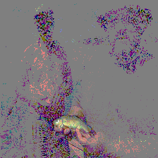
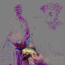
Figure 8: Illustration of different attribution objectives on an example from Imagenet labeled “tench”. Left: Original image. Middle: Top $15000$ feature attributions by Greedy PIG with the softmax objective, and Right: with the cross-entropy objective.

Specifically, instead of asking which features are most responsible for a specific classification output, we ask: Which features are most responsible for the distribution on output classes? In other words, how close is the model’s multiclass output vector when fed a subset of features versus when fed all the features? In order to answer this question, we use the loss function on which the model is trained. For multiclass classification, this is usually set to using the negative cross entropy loss $\ell(\bm{\mathit{\bar{y}}},\bm{\mathit{y}})=\langle\bm{\mathit{\bar{y}}},\log\bm{\mathit{y}}\rangle$ to define a set function $G(S)=\ell(f(\bm{\mathit{x}}),f(\bm{\mathit{x}}_{S}))$ and a corresponding continuous extension $g^{\text{logloss}}(\mathbf{s})=\ell(f(\bm{\mathit{x}}),f(\bm{\mathit{x}}\odot\mathbf{s}))$. Maximizing $G$ is equivalent to maximizing $\ell(f(\bm{\mathit{x}}),f(\bm{\mathit{x}}_{S}))$. Fortunately, gradient-based attribution algorithms can be easily extended to arbitrary objective functions. The results can be found in Figure 1 and Figure 8.

5.2 Edge-attribution to compress graphs and interpret GNNs

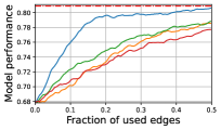
(a) Cora

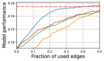
(b) Pubmed

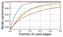
(c) ogbn-arxiv

Figure 3: Pre-trained accuracy GCN with inference using edge-subset selected by various methods. Solid lines plot accuracy vs. ratio of selected edges. Dashed line shows accuracy with all edges.

We use our method for graph compression with pre-trained GCN of Kipf and Welling (2017). We use a three-layer GCN, as:   $\textrm{GCN}(\mathcal{E};\theta)=\textbf{softmax}\left(\widehat{A_{\mathcal{E}}}\sigma\left(\widehat{A_{\mathcal{E}}}\sigma\left(\widehat{A_{\mathcal{E}}}\mathbf{X}\theta^{(1)}\right)\theta^{(2)}\right)\theta^{(3)}\right),$ where $\mathbf{X}\in\mathbb{R}^{m\times n}$ contains features of all $m$ nodes, $\mathcal{E}\subseteq[m]\times[m]$ denotes (undirected) edges with a corresponding sparse (symmetric) adjacency matrix with $(A_{\mathcal{E}})_{ij}=1$ iff in $(i,j)\in\mathcal{E}$; $\widehat{\cdot}$ is the symmetric-normalization with self-connections added, i.e., $\widehat{A}=(D+\mathbf{I}_{m})^{-\frac{1}{2}}(A+\mathbf{I}_{m})(D+\mathbf{I}_{m})^{-\frac{1}{2}}$; diagonal degree matrix $D=\textrm{diag}(\mathbf{1}_{m}^{\top}A)$; and $\sigma$ denotes element-wise non-linearity such as ReLU.

Given GCN pre-trained for node classification (Kipf and Welling, 2017; Abu-El-Haija et al., 2019; Hamilton et al., 2017), we are interested in inferring node labels using only a subset of the edges. The edge subset can be chosen uniformly at random (Fig. 3: $S_{\textrm{RND}\sim\mathcal{U}})$; or select edge $(i,j)$ with probability proportional to $(D_{ii}D_{jj})^{-\frac{1}{2}}$; or according to edge-attribution assigned by PIG (Sundararajan et al., 2017) ($S_{\textrm{PIG}})$; or using our method Greedy PIG (Alg. 1) ($S_{\textrm{GreedyPIG}}$), with

$$g^{\textrm{GNN}}(\mathbf{s};A^{(0)},A)=A^{(0)}+\mathbf{s}\odot(A-A^{(0)})\ ,\ \textrm{ \ with all-zero \ }A^{(0)}=\mathbf{0}\ ,\ \textrm{ \ and sparse \ }\mathbf{s}\in\mathbb{R}^{m\times m}.$$ (9)

Figure 3 shows that Greedy PIG can better compress the graph while maintaining performance of the underlying model. The GCN model was pre-trained on the full graph with TF-GNN (Ferludin et al., 2022), on datasets of ogbn-arxiv from Hu et al. (2020), and Cora and Pubmed from (Yang et al., 2016). Inference on the full graph (using all edges) gives performance indicated with a dashed-red line. We observe that removing $>50\%$ of the graph edges, using GreedyPIG, has negligible effect on GCN performance. For the GCN model assumptions, we ensure the selected edges $S\subseteq\mathcal{E}$ correspond to symmetric $A_{S}=A_{S}^{\top}$ by projecting the output of the gradient oracle on to the space of symmetric matrices—by averaging the (sparse) gradient with its transpose, i.e., by re-defining:

$$\widetilde{\nabla_{\mathbf{s}}g(\mathbf{s})}\overset{\triangle}{=}\frac{1}{2}\frac{\partial}{\partial\mathbf{s}}g^{\textrm{GNN}}(\mathbf{s})+\frac{1}{2}\left(\frac{\partial}{\partial\mathbf{s}}g^{\textrm{GNN}}(\mathbf{s})\right)^{\top}\ \ \ \textrm{for use in Alg.~{}\ref{alg:greedy_pig}}$$ (10)

We also use Greedy PIG to interpret the GCN. Specifically, zooming-into any particular graph node, we would like to to explain the subgraph around the node that leads to the GCN output. Due to space constraints, we report in the appendix subgraphs around nodes in the ogbn-arxiv dataset. Note that Sanchez-Lengeling et al. (2020) apply integrated gradients on smaller graphs (e.g., chemical molecules with at most 100 edges), whereas we consider large graphs (e.g., millions of edges).

5.3 Post-hoc feature selection on Criteo tabular CTR dataset

Feature selection is the task of selecting a subset of features on which to train a model, and dropping the remaining features. There are many approaches for selecting the most predictive set of features (Li et al., 2017). Even though in general feature selection and model training can be intertwined, often it is easier to decouple these processes. Specifically, given a trained model, it is often desirable to perform post-hoc feature selection, where one only has the ability to inspect and not modify the model. This is also related to global feature attribution (Zhang et al., 2021).

Methodology.

In Table 1, we compare the quality of different attribution methods for post-hoc feature selection. To evaluate the quality of feature selection, we employ the following approach: 1. Train a neural network model using all features. 2. Run each attribution method to compute global attribution scores which are aggregate attribution scores over many input examples. 3. Pick the top-$k$ attributed features, and train new pruned models that only use these top features. Report the validation loss of the resulting pruned models for different values of $k$. The results of the methodology described above applied on a random subset of the Criteo dataset are presented in Table 1. We follow the setup of Yasuda et al. (2023), who define a dense neural network with three hidden layers with sizes $768$, $256$ and $128$. To make the comparison fair, we guarantee that all algorithms consume the same amount of data (gradient batches). For example, Greedy PIG with $T=1$ steps (which we also call Sequential Gradient, see Section 3.5), uses 5x more data batches for each gradient computation than Greedy PIG with $T=5$.

Table 1: Cross-entropy loss on Criteo CTR dataset using only the top-$k$ features. Reported is the minimum validation loss after 20K training steps with batch size 512. During selection, all of the algorithms consume the same number of batches.

Algorithm	$k=5$	$k=10$	$k=20$	$k=30$
Integrated Gradients ($T=39$)	$0.4827$	$0.4641$	$0.4605$	$0.4533$
Greedy PIG ($T=1$)	$0.4728$	$0.4629$	$0.4551$	${\bf 0.4508}$
Greedy PIG ($T=5$)	${\bf 0.4723}$	${\bf 0.4627}$	${\bf 0.4531}$	$0.4509$

6 Related Work

Feature attribution, also known as computing the saliency of each feature, consists of a large class of methods for explaining the predictions of neural networks. The attribution score describes the impact of each feature on the neural network’s output. In the following, we start with most-related to our research, and then move onto broader and further topics.

Integrated gradients.

Our work is most related to (and generalizes to set functions) the work of  Sundararajan et al. (2017); Kapishnikov et al. (2021); Lundstrom et al. (2022); Qi et al. (2019); Goh et al. (2021); Sattarzadeh et al. (2021). In their seminal work, Sundararajan et al. (2017) proposed path integrated gradients (PIG), a method that assigns an importance score to each feature by integrating the partial derivative with respect to a feature along a path that interpolates between the background “baseline” and the input features. PIG, however, has some limitations. For example, it can be sensitive to the choice of baseline input. Further, it can be difficult to interpret the results of path integrated gradients when there are duplicate features or features that carry common information. It has also been observed that PIG is sensitive to input noise (Smilkov et al., 2017), model re-trains (Hooker et al., 2019), and in some cases provably unable to identify spurious features (Bilodeau et al., 2022).

Simonyan et al. (2014) used gradient ascent to explore the internal workings of neural networks and to quantify the effect of each individual pixel on the classification prediction. Springenberg et al. (2015) presented a neural network that is composed entirely of convolutional layers and introduced guided backpropagation, a technique for eliminating negative signals generated during backpropagation when performing standard gradient ascent. Grad-CAM (Selvaraju et al., 2017) produces a saliency map by using the gradients of any target concept flowing into the final convolutional layer. SmoothGrad (Smilkov et al., 2017) starts by computing the gradient of the class score function with respect to the input image. However, it visually sharpens the gradient-based sensitivity maps by adding noise to the input image and computing the gradient for each of the perturbed images. Averaging the sensitivity maps together produces a clearer result. For a comprehensive survey of feature attribution and neural network interpretability, see Zhang et al. (2021).

Shapley value.

Shapley value was originally introduced in game theory (Shapley, 1953). While it can be directly applied to explain the predictions of neural networks, it requires extremely high computational complexity. Lundberg and Lee (2017) proposed the SHapley Additive exPlanations (SHAP) algorithm, which approximates the Shapley value of features. Sundararajan and Najmi (2020) employed an axiomatic approach to investigate the differences between various versions of the Shapley value for attribution, and they also discussed a technique called Baseline Shapley (BShap). The following are other Shapley value-based methods (Chen et al., 2019; Frye et al., 2021).

Gradients and backpropgation.

Another class of interpretability methods is based on gradients and backpropagation. These methods compute the gradient of each feature, which is used as a measure of the feature’s importance (Baehrens et al., 2010; Simonyan et al., 2014). Integrated gradient is an instance of the gradient-based method. Backpropagation-based methods design backpropagation rules for convolutional, pooling, and nonlinear activation layers so they can assign importance scores in a fair and reasonable manner during backpropagation (Shrikumar et al., 2017). The guided backpropagation (GBP) algorithm (Springenberg et al., 2015), the layer-wise relevance propagation (LRP) algorithm (Bach et al., 2015), and integrated gradient (IG) algorithm (Sundararajan et al., 2017) are three notable examples of this class of methods.

Model-agnostic explanation.

Ribeiro et al. (2016) proposed Local Interpretable Model-Agnostic Explanations (LIME), a method that uses a trained local proxy model to provide explanation results without the need for backpropagation to compute gradients. Plumb et al. (2018) used a similar method that relies on a local linear model for explanation.

7 Conclusion

We view feature attribution and feature selection as instances of subset selection, which allows us to apply well-established theories and approximations from the field of discrete and submodular optimization. Through these, we give a greedy approximation using path integrated gradients (PIG), which we coin Greedy PIG. We show that Greedy PIG can succeed in scenarios where other integrated gradient methods fail, e.g., when features are correlated. We qualitatively show the efficacy of Greedy PIG—it explains predictions of ImageNet-trained model as attributions on input images, and it explains Graph Neural Network (GNN) as attributions on edges on ogbn-arxiv graph. We quantitatively evaluate Greedy PIG for feature selection on the Criteo CTR problem, and by compressing a graph by preserving only a subset of its edges while maintaining GNN performance. Our evaluations show that Greedy PIG gives qualitatively better model interpretations than alternatives, and scores higher on quantitative evaluation metrics.

Appendix A Missing Proofs

A.1 Proof of Lemma 4.3

Proof.

By Taylor’s theorem, we have

$$\nabla g(\bm{\mathit{w}})=\nabla g(\bm{\mathit{w}}_{\{i\}})+\bm{\overline{\mathit{H}}}\bm{\mathit{w}}_{[n]\backslash\{i\}}\,,$$

where $\bm{\overline{\mathit{H}}}$ is an average Hessian on the path from $\bm{\mathit{w}}$ to $\bm{\mathit{w}}_{\{i\}}$. Then,

$$\int_{t=0}^{1}\nabla_{i}g(t\mathbf{1})dt=\int_{t=0}^{1}\nabla_{i}g(t\mathbf{1}_{i})dt+\int_{t=0}^{1}\mathbf{1}_{i}^{\top}\bm{\overline{\mathit{H}}}(t)t(\mathbf{1}_{[n]\backslash\{i\}})dt$$

Now, we know that $\left|\mathbf{1}_{i}^{\top}\bm{\overline{\mathit{H}}}(t)(\mathbf{1}_{[n]\backslash\{i\}})\right|\leq K$, and $\int_{t=0}^{1}\nabla_{i}g(t\mathbf{1}_{i})dt=g(\mathbf{1}_{i})-g(\mathbf{0})$, so

$$\left|\int_{t=0}^{1}\nabla_{i}g(t\mathbf{1})dt-(g(\mathbf{1}_{i})-g(\mathbf{0}))\right|\leq K/2\,.$$

However, by the non-correlation property, this implies that

$$\nabla_{S}g(\bm{\mathit{w}})=\nabla_{S}g(\bm{\mathit{w}}_{S})$$

As a result, we have that

$$\langle\mathbf{1},\bm{\mathit{a}}_{S}\rangle =\langle\mathbf{1},-\int_{t=0}^{1}\nabla_{S}g(t\mathbf{1})dt\rangle$$

$$=\langle\mathbf{1},-\int_{t=0}^{1}\nabla_{S}g(t\mathbf{1}_{S})dt\rangle$$

$$=g(\mathbf{0})-g(\mathbf{1}_{S})\,,$$

which completes the proof. ∎

A.2 Integrated gradients for linear regression

Lemma A.1.

We consider the function $g(\bm{\mathit{w}})=-\left\|\bm{\mathit{A}}(\bm{\mathit{x}}\odot\bm{\mathit{w}})-\bm{\mathit{b}}\right\|^{2}$, where $\bm{\mathit{w}}\in[0,1]^{n}$, $\bm{\mathit{A}}\in\mathbb{R}^{m\times n}$, $\bm{\mathit{b}}\in\mathbb{R}^{m}$ and $\bm{\mathit{x}}$ is the optimal solution of the linear regression problem $\min_{\bm{\mathit{x}}}\,\left\|\bm{\mathit{A}}\bm{\mathit{x}}-\bm{\mathit{b}}\right\|^{2}$. Then, the integrated gradient scores are given by

$$\int_{t=0}^{1}\nabla g(t\mathbf{1})dt=\bm{\mathit{x}}\odot\nabla g(\mathbf{0})\,.$$

Proof.

We note that, for any $t\in[0,1]$, and using the known fact that $\bm{\mathit{x}}=(\bm{\mathit{A}}^{\top}\bm{\mathit{A}})^{+}\bm{\mathit{A}}^{\top}\bm{\mathit{b}}$, we have

$$\nabla g(t\mathbf{1}) =2\bm{\mathit{X}}^{\top}\bm{\mathit{A}}^{\top}(\bm{\mathit{A}}t\bm{\mathit{x}}-\bm{\mathit{b}})$$

$$=2t\bm{\mathit{X}}^{\top}\bm{\mathit{A}}^{\top}\bm{\mathit{b}}-2\bm{\mathit{A}}^{\top}\bm{\mathit{b}}$$

$$=-2(1-t)\bm{\mathit{X}}^{\top}\bm{\mathit{A}}^{\top}\bm{\mathit{b}}$$

$$=2(1-t)\bm{\mathit{x}}\odot\nabla g(\mathbf{0})\,,$$

where $\bm{\mathit{X}}=\mathrm{diag}(\bm{\mathit{x}})$. Then, we conclude that

$$\int_{t=0}^{1}\nabla g(t\mathbf{1})dt =2\bm{\mathit{x}}\odot\nabla g(\mathbf{0})\int_{t=0}^{1}(1-t)dt$$

$$=\bm{\mathit{x}}\odot\nabla g(\mathbf{0})\,.\qed$$

Appendix B Experimental Details and Additional Experiments

B.1 Explaining GNN predictions

For these experiments, we used GCN model pretrained on ogbn-arxiv, circa §5.2. In these experiments, we want to select graph edges that explain classification of one node (contrast to graph compression §5.2 where we select edges that maintain classification of all nodes). Given node node $i\in[m]$, we want to select neighbors of $i$, as well as their neighbors, and their neighbors, …, up-to the depth of the trained GCN (we used 3 GCN layers), that would make the GCN model prediction unchanged as compared to the full subgraph around node $i$. The gradient orcale was modified to only return nonzero gradients to edges connecting already-discovered nodes.

Figure 4 shows a qualitative evaluation of GreedyPIG. One could argue: an article should only cite another if it is related. However, the degree of relatedness can vary. When explaining GNN predictions, we hope the explanation method to select a subgraph that is very related to the center node. The figure shows that random edges around a center node can be less-related to the center node, than if the edges were chosen using GreedyPIG. In the top row of Fig. 4, MixHop paper and blue neighbors are related to GNNs and message passing (MP), whereas red nodes include embedding methods (not MP), or non-GNN applications. In the bottom row, we see that the random edge selection quickly diverged to articles within the NLP domain and otherwise unrelated applications of DeepWalk.

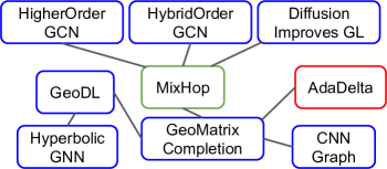
(a) GreedyPIG explains MixHop classification.

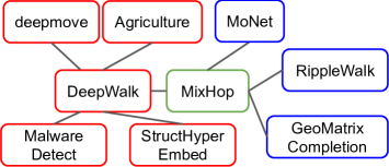
(b) Explaining w/ random edges.

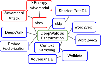
(c) GreedyPIG explains DeepWalk as … classification.

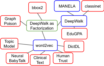
(d) Explaining w/ random edges.

Figure 4: Pre-trained Graph Neural Network (GNN) is asked to predict article category of center node (green). GreedyPIG (left column) was used to select subgraph around center node that maintains the GNN prediction and we compared it to selecting random adjacent edges. We manually labeled the selected nodes as strongly-related (blue) and less-related (red).

Finally, we shortcut the paper names to reduce visual clutter. For completeness, the full titles of the papers, as appearing in ogbn-arxiv dataset (Hu et al., 2020), are as follows.

• DeepWalk as Factorization: comprehend deepwalk as matrix factorization.

• MixHop: mixhop higher order graph convolutional architectures via sparsified neighborhood mixing.

• DeepWalk: deepwalk online learning of social representations.

• Context Sampling: vertex context sampling for weighted network embedding

• word2vec: efficient estimation of word representations in vector space

• word2vec2: distributed representations of words and phrases and their compositionality

• skip: don t walk skip online learning of multi scale network embeddings

• bbox: a restricted black box adversarial framework towards attacking graph embedding models

• AdversarialAttack: threat of adversarial attacks on deep learning in computer vision a survey

• ShortestPathDL: shortest path distance approximation using deep learning techniques.

• Walklets: walklets multiscale graph embeddings for interpretable network classification

• AdversarialE: learning graph embedding with adversarial training methods

• Embed Factorization: network embedding as matrix factorization unifying deepwalk line pte and node2vec.

• bbox: a restricted black box adversarial framework towards attacking graph embedding models

• XEntropyAdvers: cross entropy loss and low rank features have responsibility for adversarial examples"

• bbox2: the general black box attack method for graph neural networks

• HumanTrust: the transfer of human trust in robot capabilities across tasks.

• Neural BabyTalk: neural baby talk.

• DictDL: integrating dictionary feature into a deep learning model for disease named entity recognition.

• MANELA: manela a multi agent algorithm for learning network embeddings.

• ClinicalText: clinical text generation through leveraging medical concept and relations.

• EduGPA: will this course increase or decrease your gpa towards grade aware course recommendation.

• GeoMatrixCompletion: convolutional geometric matrix completion.

• GeoDL: geometric deep learning going beyond euclidean data.

• AdaDelta: adadelta an adaptive learning rate method.

• HigherOrderGCN: higher order weighted graph convolutional networks.

• HybridOrderGCN: hybrid low order and higher order graph convolutional networks.

• CNNGraph: deep convolutional networks on graph structured data.

• HyperbolicGNN: hyperbolic graph neural networks.

• deepmove: deepmove learning place representations through large scale movement data.

• Agriculture: cultivating online question routing in a question and answering community for agriculture.

• RippleWalk: ripple walk training a subgraph based training framework for large and deep graph neural network.

• MalwareDetect: aidroid when heterogeneous information network marries deep neural network for real time android malware detection.

• MoNet: monet debiasing graph embeddings via the metadata orthogonal training unit.

• StructHyperEmbed: structural deep embedding for hyper networks.

B.2 Feature attribution on images

For the experiments in Section 5.1, we used the MobilenetV2 image classification network pretrained on Imagenet, using the implementation from the tf.keras library. To implement the algorithms from previous work that we used in comparisons, i.e. integrated gradients and guided integrated gradients, we used Saliency (2017), which is an collection of implementations of state of the art saliency methods. In order to generate Figure 1, we first took a random sample of Imagenet examples from various classes, and for each sample we first applied the preprocessing routine used in MobilenetV2, which includes centering and resizing to $224\times 224$ pixels with $3$ color channels. This $224\times 224\times 3$ tensor of $3$ dimensions is the input to the neural network, and as a result it is also the shape of the attribution map.

We ran different attribution algorithms and sorted the absolute values of attribution values. Then, we picked $100$ equally spaced values for $k$, from $0$ to $224\cdot 224\cdot 3$, and generated an image using only the top-$k$ attribution values (and replacing the rest by the baseline, which in this case is a gray image). For guided PIG and SmoothGrad, we used the default settings from the saliency library.

B.3 Pointing game

In this section, we consider the pointing game defined by Bohle et al. (2021); Böhle et al. (2022), which is a sanity check for the usefulness of feature attribution methods on images. In this game, examples of different classes are stitched together in a grid to form a new image. Then, this new image is fed to the attribution method, with the goal to explain one of the four classes. Ideally, the highest attributions should be concentrated in the quadrant that corresponds to the selected class. In Figures 5 and 6, we see one such example that compares the attributions of integrated gradients and Greedy PIG.

Input image

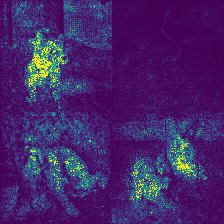
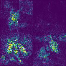
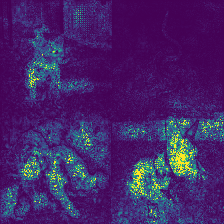
Top 15000 Integrated Gradient attributions for each class.

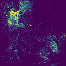
schipperke

sea snake

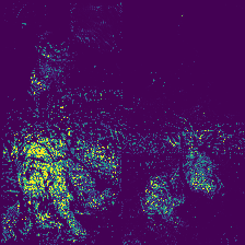
otterhound

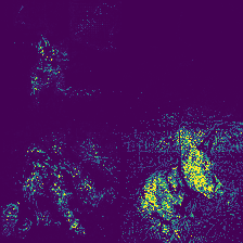
Cardigan

Top 15000 Greedy PIG attributions for each class.

Figure 5: The input image is generated as a $2\times 2$ grid of images from different classes, here schipperke, sea snake, otterhound and Cardigan. Ideally, attributions should be concentrated in the quadrant associated with the respective class.

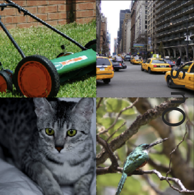
Input image

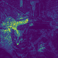
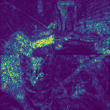
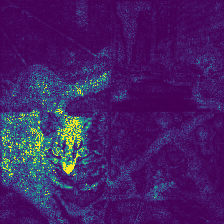
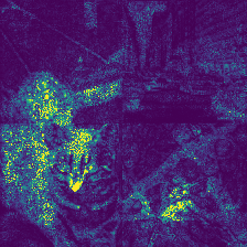
Top 15000 Integrated Gradient attributions for each class.

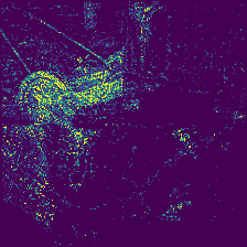
lawnmower

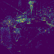
cab

Egyptian cat

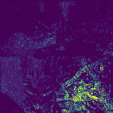
jacamar

Top 15000 Greedy PIG attributions for each class.

Figure 6: The input image is generated as a $2\times 2$ grid of images from different classes, here lawnmower, cab, Egyptian cat and jacamar. Ideally, attributions should be concentrated in the quadrant associated with the respective class.

B.4 Examples

B.5 Block-wise feature attribution

In the spirit of Kapishnikov et al. (2019), we augment the greedy PIG algorithm with the ability to select patches instead of individual features from a $3$-dimensional image tensor. In fact, our implementation allows for specifying arbitrary subset structures that are to be selected as individual features. The results can be found in Figure 9.

To get into more detail, the approach of Kapishnikov et al. (2019) is to first compute attribution scores using integrated gradients, and then iteratively find regions of the image with maximum sum of attributions. The main difference from our approach, is that we invoke the integrated gradient algorithm after every block selection, insteado of just once, in line with our adaptive approach. Specifically, for a given block size $b\times b$, after each round of greedy PIG we compute the $b\times b$ patch with the maximum sum of attributions, and select this patch. It should be noted that selected features have a score of $0$ in future iterations.

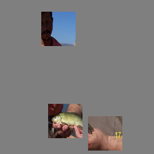
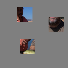
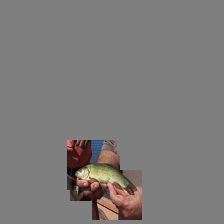
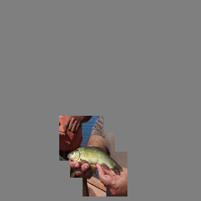
(a) Block-wise attributions. From left to right: Integrated gradients with softmax, integrated gradients with cross entropy, greedy PIG with softmax, greedy PIG with cross entropy.

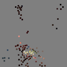
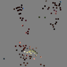
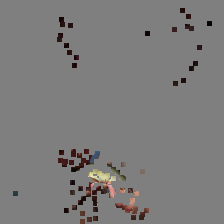
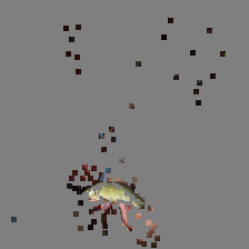
(b) Block-wise attributions. From left to right: Integrated gradients with softmax, greedy PIG with softmax, integrated gradients with cross entropy, greedy PIG with cross entropy.

Figure 9: Illustration of different attribution objectives on an example from Imagenet labeled “tench”, with different block sizes.

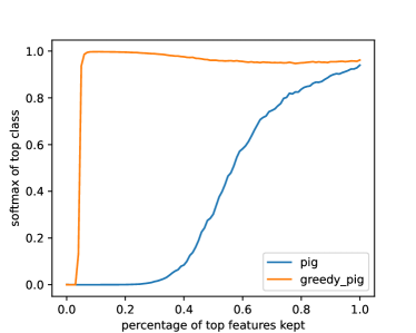
Figure 10: Comparing PIG and Greedy PIG on ImageNet attribution using ResNet50. The AUC scores for PIG and Greedy PIG are $0.39443$ and $0.9262$ respectively.

B.6 Feature selection

For the experiments in Section 5.3, we used a model identical to Yasuda et al. (2023), which is a $3$-hidden layer neural network with ReLU activations. We implemented minibatch versions of integrated gradients and greedy PIG.

Note:

While the attributions computed by the integrated gradients algorithm can be averaged over the whole dataset to compute global attribution scores, this is not necessarily the case with the greedy PIG attribution scores. This is another place where the formulation in Definition 4.1 will be handy. Specifically, given a model $f(\cdot;\bm{\mathit{\theta}})$ with parameters $\bm{\mathit{\theta}}$, data $(\bm{\mathit{X}},\bm{\mathit{y}})$ and an aggregate loss function $\ell$ over the data, we define the post-hoc feature selection problem simply by $G(S):=-\ell(\bm{\mathit{y}},f(\bm{\mathit{X}}_{S};\bm{\mathit{\theta}}))$. Note that this is not equivalent to averaging the greedy PIG attributions across the dataset. While a naive implementation of Algorithm 1 would require multiple full batch gradient evaluations in each round, we implement a mini-batch version, which instead samples a number of data batches in each round, and computes the gradient over these batches.

Specifically, given a number $n=150000$ of available data batches, each of size $512$, and a number $g=39$ of gradients to be evaluated (this is the number of integrated gradient steps), we randomly shuffle the batches and evaluate each of the gradients on a random set of $n/g\approx 3846$ batches (i.e. the gradient is averaged over all these batches). In this way, we can ensure that all algorithms use the same amount of data, and the algorithms are scalable enough to be used in large scale settings.

References

- Abebe et al. (2022) Rediet Abebe, Moritz Hardt, Angela Jin, John Miller, Ludwig Schmidt, and Rebecca Wexler. Adversarial scrutiny of evidentiary statistical software. In 2022 ACM Conference on Fairness, Accountability, and Transparency, FAccT ’22, page 1733–1746, 2022.
- Abu-El-Haija et al. (2019) Sami Abu-El-Haija, Bryan Perozzi, Amol Kapoor, Hrayr Harutyunyan, Nazanin Alipourfard, Kristina Lerman, Greg Ver Steeg, and Aram Galstyan. Mixhop: Higher-order graph convolutional architectures via sparsified neighborhood mixing. In International Conference on Machine Learning, ICML, 2019.
- Adebayo et al. (2018) Julius Adebayo, Justin Gilmer, Michael Muelly, Ian Goodfellow, Moritz Hardt, and Been Kim. Sanity checks for saliency maps. Advances in neural information processing systems, 31, 2018.
- Ahmad et al. (2018) Muhammad Aurangzeb Ahmad, Carly Eckert, and Ankur Teredesai. Interpretable machine learning in healthcare. In Proceedings of the 2018 ACM International Conference on Bioinformatics, Computational Biology, and Health Informatics, pages 559–560, 2018.
- Ancona et al. (2017) Marco Ancona, Enea Ceolini, Cengiz Öztireli, and Markus Gross. Towards better understanding of gradient-based attribution methods for deep neural networks. arXiv preprint arXiv:1711.06104, 2017.
- Axiotis and Yasuda (2023) Kyriakos Axiotis and Taisuke Yasuda. Performance of regularization for sparse convex optimization. arXiv preprint arXiv:2307.07405, 2023.
- Bach et al. (2015) Sebastian Bach, Alexander Binder, Grégoire Montavon, Frederick Klauschen, Klaus-Robert Müller, and Wojciech Samek. On pixel-wise explanations for non-linear classifier decisions by layer-wise relevance propagation. PloS one, 10(7):e0130140, 2015.
- Baehrens et al. (2010) David Baehrens, Timon Schroeter, Stefan Harmeling, Motoaki Kawanabe, Katja Hansen, and Klaus-Robert Müller. How to explain individual classification decisions. The Journal of Machine Learning Research, 11:1803–1831, 2010.
- Balkanski and Singer (2018) Eric Balkanski and Yaron Singer. The adaptive complexity of maximizing a submodular function. In Proceedings of the 50th Annual ACM SIGACT Symposium on Theory of Computing, pages 1138–1151, 2018.
- Bateni et al. (2019) MohammadHossein Bateni, Lin Chen, Hossein Esfandiari, Thomas Fu, Vahab Mirrokni, and Afshin Rostamizadeh. Categorical feature compression via submodular optimization. In International Conference on Machine Learning, pages 515–523. PMLR, 2019.
- Bilodeau et al. (2022) Blair Bilodeau, Natasha Jaques, Pang Wei Koh, and Been Kim. Impossibility theorems for feature attribution. arXiv preprint arXiv:2212.11870, 2022.
- Bohle et al. (2021) Moritz Bohle, Mario Fritz, and Bernt Schiele. Convolutional dynamic alignment networks for interpretable classifications. In Proceedings of the IEEE/CVF Conference on Computer Vision and Pattern Recognition, pages 10029–10038, 2021.
- Böhle et al. (2022) Moritz Böhle, Mario Fritz, and Bernt Schiele. B-cos networks: Alignment is all we need for interpretability. In Proceedings of the IEEE/CVF Conference on Computer Vision and Pattern Recognition, pages 10329–10338, 2022.
- Bubeck et al. (2023) Sébastien Bubeck, Varun Chandrasekaran, Ronen Eldan, Johannes Gehrke, Eric Horvitz, Ece Kamar, Peter Lee, Yin Tat Lee, Yuanzhi Li, Scott Lundberg, et al. Sparks of artificial general intelligence: Early experiments with GPT-4. arXiv preprint arXiv:2303.12712, 2023.
- Cai et al. (2018) Jie Cai, Jiawei Luo, Shulin Wang, and Sheng Yang. Feature selection in machine learning: A new perspective. Neurocomputing, 300:70–79, 2018.
- Chen et al. (2021a) Irene Y Chen, Emma Pierson, Sherri Rose, Shalmali Joshi, Kadija Ferryman, and Marzyeh Ghassemi. Ethical machine learning in healthcare. Annual Review of Biomedical Data Science, 4:123–144, 2021a.
- Chen et al. (2019) Jianbo Chen, Le Song, Martin J Wainwright, and Michael I Jordan. L-shapley and c-shapley: Efficient model interpretation for structured data. In International Conference on Learning Representations, 2019.
- Chen et al. (2021b) Lin Chen, Hossein Esfandiari, Gang Fu, Vahab S Mirrokni, and Qian Yu. Feature cross search via submodular optimization. In 29th Annual European Symposium on Algorithms (ESA 2021). Schloss Dagstuhl-Leibniz-Zentrum für Informatik, 2021b.
- Elenberg et al. (2018) Ethan R Elenberg, Rajiv Khanna, Alexandros G Dimakis, and Sahand Negahban. Restricted strong convexity implies weak submodularity. The Annals of Statistics, 46(6B):3539–3568, 2018.
- Fahrbach et al. (2019a) Matthew Fahrbach, Vahab Mirrokni, and Morteza Zadimoghaddam. Non-monotone submodular maximization with nearly optimal adaptivity and query complexity. In International Conference on Machine Learning, pages 1833–1842. PMLR, 2019a.
- Fahrbach et al. (2019b) Matthew Fahrbach, Vahab Mirrokni, and Morteza Zadimoghaddam. Submodular maximization with nearly optimal approximation, adaptivity and query complexity. In Proceedings of the Thirtieth Annual ACM-SIAM Symposium on Discrete Algorithms, pages 255–273. SIAM, 2019b.
- Ferludin et al. (2022) Oleksandr Ferludin, Arno Eigenwillig, Martin Blais, Dustin Zelle, Jan Pfeifer, Alvaro Sanchez-Gonzalez, Sibon Li, Sami Abu-El-Haija, Peter Battaglia, Neslihan Bulut, et al. TF-GNN: Graph neural networks in tensorflow. arXiv preprint arXiv:2207.03522, 2022.
- Frye et al. (2021) Christopher Frye, Damien de Mijolla, Tom Begley, Laurence Cowton, Megan Stanley, and Ilya Feige. Shapley explainability on the data manifold. In International Conference on Learning Representations, 2021.
- Goh et al. (2021) Gary SW Goh, Sebastian Lapuschkin, Leander Weber, Wojciech Samek, and Alexander Binder. Understanding integrated gradients with smoothtaylor for deep neural network attribution. In 2020 25th International Conference on Pattern Recognition (ICPR), pages 4949–4956. IEEE, 2021.
- Graves et al. (2013) Alex Graves, Abdel-rahman Mohamed, and Geoffrey Hinton. Speech recognition with deep recurrent neural networks. In 2013 IEEE international conference on acoustics, speech and signal processing, pages 6645–6649. Ieee, 2013.
- Hamilton et al. (2017) W. Hamilton, R. Ying, and J. Leskovec. Inductive representation learning on large graphs. In Advances in Neural Information Processing Systems, 2017.
- He et al. (2016) Kaiming He, Xiangyu Zhang, Shaoqing Ren, and Jian Sun. Deep residual learning for image recognition. In Proceedings of the IEEE conference on computer vision and pattern recognition, pages 770–778, 2016.
- Hooker et al. (2019) Sara Hooker, Dumitru Erhan, Pieter-Jan Kindermans, and Been Kim. A benchmark for interpretability methods in deep neural networks. Advances in neural information processing systems, 32, 2019.
- Hu et al. (2020) Weihua Hu, Matthias Fey, Marinka Zitnik, Yuxiao Dong, Hongyu Ren, Bowen Liu, Michele Catasta, and Jure Leskovec. Open graph benchmark: Datasets for machine learning on graphs. In arXiv, 2020.
- Kapishnikov et al. (2019) Andrei Kapishnikov, Tolga Bolukbasi, Fernanda Viégas, and Michael Terry. Xrai: Better attributions through regions. In Proceedings of the IEEE/CVF International Conference on Computer Vision, pages 4948–4957, 2019.
- Kapishnikov et al. (2021) Andrei Kapishnikov, Subhashini Venugopalan, Besim Avci, Ben Wedin, Michael Terry, and Tolga Bolukbasi. Guided integrated gradients: An adaptive path method for removing noise. In Proceedings of the IEEE/CVF Conference on Computer Vision and Pattern Recognition, pages 5050–5058, 2021.
- Kipf and Welling (2017) Thomas Kipf and Max Welling. Semi-supervised classification with graph convolutional networks. In International Conference on Learning Representations, 2017.
- Kleindessner et al. (2019) Matthäus Kleindessner, Pranjal Awasthi, and Jamie Morgenstern. Fair k-center clustering for data summarization. In International Conference on Machine Learning, pages 3448–3457. PMLR, 2019.
- Krause and Golovin (2014) Andreas Krause and Daniel Golovin. Submodular function maximization. Tractability, 3:71–104, 2014.
- Krizhevsky et al. (2017) Alex Krizhevsky, Ilya Sutskever, and Geoffrey E Hinton. Imagenet classification with deep convolutional neural networks. Communications of the ACM, 60(6):84–90, 2017.
- Li et al. (2017) Jundong Li, Kewei Cheng, Suhang Wang, Fred Morstatter, Robert P Trevino, Jiliang Tang, and Huan Liu. Feature selection: A data perspective. ACM computing surveys (CSUR), 50(6):1–45, 2017.
- Liberty and Sviridenko (2017) Edo Liberty and Maxim Sviridenko. Greedy minimization of weakly supermodular set functions. In Approximation, Randomization, and Combinatorial Optimization. Algorithms and Techniques (APPROX/RANDOM 2017). Schloss Dagstuhl-Leibniz-Zentrum fuer Informatik, 2017.
- Liu et al. (2023) Lydia T. Liu, Serena Wang, Tolani Britton, and Rediet Abebe. Reimagining the machine learning life cycle to improve educational outcomes of students. Proceedings of the National Academy of Sciences, 120(9):e2204781120, 2023.
- Lundberg and Lee (2017) Scott M Lundberg and Su-In Lee. A unified approach to interpreting model predictions. Advances in neural information processing systems, 30, 2017.
- Lundstrom et al. (2022) Daniel D Lundstrom, Tianjian Huang, and Meisam Razaviyayn. A rigorous study of integrated gradients method and extensions to internal neuron attributions. In International Conference on Machine Learning, pages 14485–14508. PMLR, 2022.
- Mirrokni and Zadimoghaddam (2015) Vahab Mirrokni and Morteza Zadimoghaddam. Randomized composable core-sets for distributed submodular maximization. In Proceedings of the forty-seventh annual ACM Symposium on Theory of Computing, pages 153–162, 2015.
- Nemhauser et al. (1978) George L Nemhauser, Laurence A Wolsey, and Marshall L Fisher. An analysis of approximations for maximizing submodular set functions—i. Mathematical programming, 14:265–294, 1978.
- Plumb et al. (2018) Gregory Plumb, Denali Molitor, and Ameet S Talwalkar. Model agnostic supervised local explanations. Advances in neural information processing systems, 31, 2018.
- Qi et al. (2019) Zhongang Qi, Saeed Khorram, and Fuxin Li. Visualizing deep networks by optimizing with integrated gradients. In CVPR Workshops, volume 2, pages 1–4, 2019.
- Ribeiro et al. (2016) Marco Tulio Ribeiro, Sameer Singh Singh, and Carlos Guestrin. Model-agnostic interpretability of machine learning. In Proceedings of the 2016 ICML Workshop on Human Interpretability in Machine Learning (WHI 2016). New York, NY, 2016.
- Saliency (2017) Saliency. Framework-agnostic implementation for state-of-the-art saliency methods (xrai, blurig, smoothgrad, and more). https://github.com/PAIR-code/saliency, 2017.
- Sanchez-Lengeling et al. (2020) Benjamin Sanchez-Lengeling, Jennifer Wei, Brian Lee, Emily Reif, Peter Wang, Wesley Qian, Kevin McCloskey, Lucy Colwell, and Alexander Wiltschko. Evaluating attribution for graph neural networks. In Advances in Neural Information Processing Systems, volume 33, pages 5898–5910, 2020.
- Sandler et al. (2018) Mark Sandler, Andrew Howard, Menglong Zhu, Andrey Zhmoginov, and Liang-Chieh Chen. Mobilenetv2: Inverted residuals and linear bottlenecks. In Proceedings of the IEEE conference on computer vision and pattern recognition, pages 4510–4520, 2018.
- Sattarzadeh et al. (2021) Sam Sattarzadeh, Mahesh Sudhakar, Konstantinos N Plataniotis, Jongseong Jang, Yeonjeong Jeong, and Hyunwoo Kim. Integrated grad-cam: Sensitivity-aware visual explanation of deep convolutional networks via integrated gradient-based scoring. In ICASSP 2021-2021 IEEE International Conference on Acoustics, Speech and Signal Processing (ICASSP), pages 1775–1779. IEEE, 2021.
- Selvaraju et al. (2017) Ramprasaath R Selvaraju, Michael Cogswell, Abhishek Das, Ramakrishna Vedantam, Devi Parikh, and Dhruv Batra. Grad-cam: Visual explanations from deep networks via gradient-based localization. In Proceedings of the IEEE international conference on computer vision, pages 618–626, 2017.
- Shapley (1953) Lloyd S Shapley. A value for n-person games. Contributions to Theory Games (AM-28), 1953.
- Shrikumar et al. (2017) Avanti Shrikumar, Peyton Greenside, and Anshul Kundaje. Learning important features through propagating activation differences. In International conference on machine learning, pages 3145–3153. PMLR, 2017.
- Simonyan et al. (2014) K Simonyan, A Vedaldi, and A Zisserman. Deep inside convolutional networks: visualising image classification models and saliency maps. In Proceedings of the International Conference on Learning Representations (ICLR). ICLR, 2014.
- Smilkov et al. (2017) Daniel Smilkov, Nikhil Thorat, Been Kim, Fernanda Viégas, and Martin Wattenberg. Smoothgrad: removing noise by adding noise. arXiv preprint arXiv:1706.03825, 2017.
- Springenberg et al. (2015) J Springenberg, Alexey Dosovitskiy, Thomas Brox, and M Riedmiller. Striving for simplicity: The all convolutional net. In ICLR (workshop track), 2015.
- Sundararajan and Najmi (2020) Mukund Sundararajan and Amir Najmi. The many shapley values for model explanation. In International conference on machine learning, pages 9269–9278. PMLR, 2020.
- Sundararajan et al. (2017) Mukund Sundararajan, Ankur Taly, and Qiqi Yan. Axiomatic attribution for deep networks. In International conference on machine learning, pages 3319–3328. PMLR, 2017.
- Wiens and Shenoy (2018) Jenna Wiens and Erica S Shenoy. Machine learning for healthcare: on the verge of a major shift in healthcare epidemiology. Clinical Infectious Diseases, 66(1):149–153, 2018.
- Xu et al. (2020) Shawn Xu, Subhashini Venugopalan, and Mukund Sundararajan. Attribution in scale and space. In Proceedings of the IEEE/CVF Conference on Computer Vision and Pattern Recognition, pages 9680–9689, 2020.
- Yang et al. (2016) Zhilin Yang, William W Cohen, and Ruslan Salakhutdinov. Revisiting semi-supervised learning with graph embeddings. In International Conference on Machine Learning, 2016.
- Yasuda et al. (2023) Taisuke Yasuda, MohammadHossein Bateni, Lin Chen, Matthew Fahrbach, Gang Fu, and Vahab Mirrokni. Sequential attention for feature selection. ICLR 2023, 2023.
- Zhang et al. (2021) Yu Zhang, Peter Tiňo, Aleš Leonardis, and Ke Tang. A survey on neural network interpretability. IEEE Transactions on Emerging Topics in Computational Intelligence, 5(5):726–742, 2021.