Syntax-semantics interface: an algebraic model

Abstract.

We extend our formulation of Merge and Minimalism in terms of Hopf algebras to an algebraic model of a syntactic-semantic interface. We show that methods adopted in the formulation of renormalization (extraction of meaningful physical values) in theoretical physics are relevant to describe the extraction of meaning from syntactic expressions. We show how this formulation relates to computational models of semantics and we answer some recent controversies about implications for generative linguistics of the current functioning of large language models.

1. Introduction: modelling the syntax-semantics interface

The modelling of the generative process of syntax, based on the core computational structure of Merge, within the setting of the Minimalist Model, satisfies the following fundamental properties:

1. a concise conceptual framework;

2. a precise mathematical formulation;

3. good explanatory power.

For the most recent formulation of Minimalism, the first and third property are articulated in [13], [14], [15] and in the upcoming [16]. While the requirement of the existence of precise mathematical models has been traditionally associated to sciences like physics, the fact that syntax is essentially a computational process suggests that a mathematical formulation should also be a desirable requirement in linguistics, and more specifically in the modelling of I-language. We presented a detailed mathematical model of syntactic Merge in our previous papers [61] and [62].

In comparison with syntax, the modeling of semantics is presently in a less satisfactory state from the point of view of the same three properties listed above. Some main approaches to semantics include forms of compositional semantics [73], [74], truth-conditional semantics, semiring semantics [36], and vector-space models (the latter especially in computational linguistics). General views of logic-oriented approaches to semantics, which we will not be discussing in this paper, can be seen, for instance, in [78], [82], [86]. Each of these viewpoints has limitations of a different nature.

Our purpose here is not to carry out a comprehensive comparative analysis and criticism of contemporary models of semantics. Rather, we want to approach the problem of modeling the syntactic-semantic interface on the basis of a list of abstract properties, and articulate a possible mathematical setting that such properties suggest. We can then compare existing models with the specific structure that we identify. We will show that one can remain, to some extent, agnostic about specific models of semantics, beyond some basic requirements, and still retain a fundamental functioning model of the interaction with syntax. This reflects a view of the syntax-semantics interface that is primarily syntax-driven.

As in the case of our mathematical formulation of Merge in terms of Hopf algebras, our guiding principle will be an analogy with conceptually similar structures that arise in theoretical physics. In particular, in the context of fundamental physical interactions described by the quantum field theory, fundamental problem is the assignment of “meaningful” physical values to the computation of the expectation values of the theory. This can be compared with the assignment of meaning–semantics–to syntactic objects. More precisely, assignment of meaning the quantum field theory setting consists of the extraction of a finite (meaningful) part from Feynman integrals that are in general divergent (produce meaningless infinities). This process is known in theoretical physics as renormalization. While the renormalization problem and procedures leading to satisfactory solutions for it have been known to physicists since the development of quantum electrodynamics in the 1950s and 60s (see [6]), a complete understanding of the underlying mathematical structure is much more recent, (see [20], [21]).

Even more recently, it has been shown shown that the same mathematical formalism can be applied in the theory of computation, in order to extract, in a similar way, computable “subfunctions” from non-decidable problems (undecidability being the analog in the theory of computation of the unphysical infinities); see [54], [55], and also [23].

Assuming the conceptual standpoint that Internal or I-language is, in essence, a computational process, the extension of the mathematical framework of renormalization to the theory of computation suggests the existence of a similar possible manifestation in linguistics as well. In the case of linguistics, one does not have to deal with divergences (of a physical or computational nature); rather one has to carry out a consistent assignment of meaning to syntactic objects produced by the Merge mechanism, and reject inconsistencies and impossibilities. In the rest of this paper we plan to turn this heuristic comparison into a precise formulation.

There are several reasons why developing such a mathematical model of the syntax-semantics interface is desirable. Aside from general principles based on the three “good properties” of theoretical modeling stated above, there are other possible applications of interest. For instance, a significant ongoing debate and controversy has ensued from the recent development of large language models, with various claims of incompatibility with, or “disproval” of the generative linguistics framework itself. Since such theories, in our view, ultimately describe computational processes (albeit most likely also in our view of a different nature from those governing language in human brains), a viable computational and mathematical setting is required, where a specific comparative analysis can be carried out, and such claims can be addressed.

1.1. Some conceptual requirements for a syntax-semantics interface

We start our analysis by setting out a simple list of what we regard as desirable properties of a model of the syntax-semantic interface.

1. Autonomy of syntax

2. Syntax supports semantic interpretation

3. Semantic interpretation is, to a large extent, independent of externalization

4. Compositionality

The first requirement, the autonomy of syntax, expresses that the computational generative process of syntax described by Merge is independent of semantics. The second requirement can be seen as positing that the syntax-semantic interface proceeds from syntax to semantics (a syntax-first view), while syntax itself is not semantic in nature. The third claim separates the interaction of the core computational mechanism of syntax with a Conceptual-Intentional system, which gives rise to the syntax-semantic interface, from the interaction with an Articulatory-Perceptual or Sensory-Motor system, which includes the process of externalization. While it is reasonable to assume a certain level of interaction between these two mechanisms, with “independence of externalization” we emphasize that semantic interpretation depends primarily on structural relations and proximity in the syntactic structure rather than on linear proximity of words in a sentence. The compositional property is meant here simply as a requirement of consistency across syntactic sub-structures.

We also add another general principle that we will try to incorporate in our model and that may be at odds with some of the traditional approaches to semantics (such as the truth value based approaches). We propose the following fundamental distinction between the roles of syntax and semantics in language

• Syntax is a computational process.

• Semantics is not a computational process and is in essence grounded on a notion of topological proximity.

The first statement is clear in the context of generative linguistics, and in particular in the setting of Minimalism, where the computational process is run by the fundamental operation Merge. The second assertion requires some contextual clarification. Saying that semantics is only endowed with a notion of proximity of a topological nature does not mean that it is not possible, or desirable, to consider models of semantics where additional structure is present, but rather that these additional properties (metric, linear, semiring structures, for instance) only play a role to instantiate or quantify proximity relations. The compositionality of semantics does not require positing an additional computational structure on semantics itself: the computational structure of syntax suffices to induce it. In this view, semantics is not really a part of language itself, but rather an autonomous structure that deals with proximity classifications.

1.2. Syntax

On the syntax side of the syntax-semantic interface we assume the formulation of free symmetric Merge presented in [61]. This accounts for the properties (1) and (3) in our list of §1.1: it provides a computational model of syntax that is independent of semantics, and where the interface with semantics takes place at the level of the free symmetric Merge, without requiring prior externalization. Free symmetric Merge generates syntactic objects, described by binary rooted trees without any assigned planar embedding. Thus, our choice of modeling the syntax-semantic interface starting from the level of free symmetric Merge as the syntactic part of the interface, has the effect of ensuring that the interface of syntax and semantics (also sometimes called the Conceptual-Intentional system) is parallel and separate from the channel connecting the output of Merge to externalization (the so-called Articulatory-Perceptual system), although interactions between these two channels can be incorporated in the model (and will be discussed in §4 of this paper).

Summarizing the setting of [61], syntax is represented by the following data:

• a (finite) set ${\mathcal{S}}{\mathcal{O}}_{0}$ of lexical items and syntactic features;

• the set of syntactic objects ${\mathcal{S}}{\mathcal{O}}$, identified with the set ${\mathfrak{T}}_{{\mathcal{S}}{\mathcal{O}}_{0}}$ of binary rooted trees (with no planar structure) with leaves labeled by ${\mathcal{S}}{\mathcal{O}}_{0}$, generated as the free, non-associative, commutative magma over the set ${\mathcal{S}}{\mathcal{O}}_{0}$,

  (1.1) $${\mathcal{S}}{\mathcal{O}}={\rm Magma}_{na,c}({\mathcal{S}}{\mathcal{O}}_{0},{\mathfrak{M}})={\mathfrak{T}}_{{\mathcal{S}}{\mathcal{O}}_{0}}\,;$$

• the set of accessible terms of a syntactic object $T\in{\mathfrak{T}}_{{\mathcal{S}}{\mathcal{O}}_{0}}$, given by the set of all the full subtrees $T_{v}\subset T$ with root a non-root vertex $v\in V(T)$;

• the commutative Hopf algebra of workspaces given by the vector space ${\mathcal{V}}({\mathfrak{F}}_{{\mathcal{S}}{\mathcal{O}}_{0}})$ spanned by the set ${\mathfrak{F}}_{{\mathcal{S}}{\mathcal{O}}_{0}}$ of (finite) binary rooted forests with leaves decorated by elements of the set ${\mathcal{S}}{\mathcal{O}}_{0}$, with product given by the disjoint union $\sqcup$ and coproduct determined by

  (1.2) $$\Delta(T)=T\otimes 1+1\otimes T+\sum_{v}F_{\underline{v}}\otimes T/F_{\underline{v}}\,,$$

  with $F_{\underline{v}}=T_{v_{q}}\sqcup\cdots\sqcup T_{v_{n}}$ a collection of accessible terms;

• the action of Merge on workspaces

  $${\mathfrak{M}}=\sqcup\circ({\mathfrak{B}}\otimes{\rm id})\circ\Delta$$

  where ${\mathcal{B}}$ is the grafting of components of a forest to a common root vertex, or for a fixed pair of syntactic objects $S,S^{\prime}$

  (1.3) $${\mathfrak{M}}_{S,S^{\prime}}=\sqcup\circ({\mathfrak{B}}\otimes{\rm id})\circ\delta_{S,S^{\prime}}\circ\Delta\,,$$

  where $\delta_{S,S^{\prime}}$ selects matching pairs in the workspace (see [61] for a more detailed description).

We will use the notation ${\mathcal{H}}=({\mathcal{V}}({\mathfrak{F}}_{{\mathcal{S}}{\mathcal{O}}_{0}}),\sqcup,\Delta,S)$ for the Hopf algebra described above. Note that since the Hopf algebra is graded, the antipode $S$ is defined inductively using the coproduct, so that we can equivalently just specify the bialgebra part of the structure, ${\mathcal{H}}=({\mathcal{V}}({\mathfrak{F}}_{{\mathcal{S}}{\mathcal{O}}_{0}}),\sqcup,\Delta)$.

1.2.1. Remark on the Hopf algebra coproduct

We pointed out in [61] that there are two possible ways of interpreting the quotient $T/T_{v}$ (or more generally $T/F_{\underline{v}}$) in the coproduct (1.2), either as contraction of $T_{v}$ to its root vertex or as deletion of $T_{v}$ (and taking the unique maximal binary tree determined by the complement). In [61] we argued that, if one wants to avoid having to introduce labeling algorithms for the internal vertices of the trees, and only have the leaves labelled by lexical items and syntactic features in ${\mathcal{S}}{\mathcal{O}}_{0}$, then the second procedure is preferable.

However, when it comes to interfacing syntax with semantics, it is in fact better to retain the root vertex $v$ of $T_{v}$ in the quotient $T/T_{v}$ as that provides so-called traces, the empty categories left behind by “movement” implemented by so-called Internal Merge. As is familiar from the long historical discussion of what is called reconstruction, the trace is needed for semantic parsing, so in the context we consider here we will be using the quotient $T/T_{v}$ where $T_{v}$ is contracted to its root, marked as trace. Similarly, in quotients $T/F_{\underline{v}}$ each tree component $T_{v_{i}}$ of the forest $F_{\underline{v}}$ is contracted to its root vertex $v_{i}$.

1.2.2. A comment about Tree Adjoining Grammars – TAGs

Since readers of our previous papers [61], [62] have occasionally asked this question, we add here a very brief clarification on the difference between the algebraic structure of Merge described in [61] and that of tree adjoining grammars (TAGs). In the setting of TAGs, one considers a generative process that depends on an initial choice of a given finite set of “elementary trees” with vertex labels. In TAGs, in general, trees are not necessarily assumed to be binary. There are two composition rules: one composition operation (substitution rule) consists of grafting the root of a tree to the leaf of another tree; a second composition operation (a so-called adjoining rule) inserts at an internal vertex of a tree with a label $x$ another tree with root labeled by $x$, and one of the leaves also labeled by $x$. The adjoining rule can be obtained as a suitable composition of grafting of roots to leaves, so the basic generative operations of TAGs are the operad compositions of rooted trees. Namely, if ${\mathcal{O}}(n)$ denotes the set of trees in a given TAG with $n$ leaves, then there are composition maps

(1.4) $$\circ_{i}:{\mathcal{O}}(n)\times{\mathcal{O}}(m)\to{\mathcal{O}}(n+m-1)$$

that plug the root of a tree in ${\mathcal{O}}(n)$ to the $i$-th leaf of a tree in ${\mathcal{O}}(m)$ resulting in a tree in ${\mathcal{O}}(n+m-1)$. Such operations, subject to associativity and unitarity conditions, define the algebraic structure of an operad. Label matching conditions may require partial operads, but we will not discuss this here.

In order to compare the TAG formalism with the algebraic formulation of Merge of [61], one should note that there is an important relation between the two as well as important differences: the latter show that these two formalisms do not constitute the same algebraic structure. This is why, in our view, it is algebraic structure that is essential to the line of work presented here, rather than the formal language theoretic notion of weak generative capacity (such as mild-context sensitivity).

The relation between TAGs and Merge arises from the fact that, in the Merge formalism of [61], recalled in §1.2 above, the syntactic objects $T\in{\mathcal{S}}{\mathcal{O}}={\mathfrak{T}}_{{\mathcal{S}}{\mathcal{O}}_{0}}$ are generated as elements of the free non-associative commutative magma (1.1) on the Merge operation ${\mathfrak{M}}$. This does have an equivalent operad formulation, in terms of the quadratic operad freely generated by the single commutative binary operation ${\mathfrak{M}}$, see [43]. Thus, there exists an equivalent way of formulating the generative process for the syntactic objects in terms of operad compositions (1.4), that makes this generative process appear similar to TAGs. However, the main difference between the two lies in the fact that the Merge formalism does not just consist of the generation of syntactic objects through the magma operation, but also of the action of Merge on so-called workspaces, given by forests $F\in{\mathfrak{T}}_{{\mathcal{S}}{\mathcal{O}}_{0}}$.

The action of Merge on workspaces is not determined only by the operad underlying the ${\mathcal{S}}{\mathcal{O}}$ magma, but also requires the additional datum of the Hopf algebra structure on workspaces. This makes it possible to incorporate not just so-called External Merge, that is involved in the magma ${\mathcal{S}}{\mathcal{O}}$, but also Internal Merge, that requires an additional coproduct operation.

It is important to observe here that the operad underlying ${\mathcal{S}}{\mathcal{O}}$ also determines a Hopf algebra, the associative, commutative Hopf algebra on the vector space ${\mathcal{V}}({\mathfrak{F}}_{{\mathcal{S}}{\mathcal{O}}_{0}})$ spanned by forests of binary rooted trees, used in [61] to formulate the action of Merge on workspaces. However, this is not the same as the non-associative, commutative Hopf algebra structure induced by the operad on the vector space ${\mathcal{V}}({\mathfrak{T}}_{{\mathcal{S}}{\mathcal{O}}_{0}})$ spanned by binary rooted trees as in TAGs; see [44], [45]. This is the key algebraic difference between TAGs and Merge. The introduction of workspaces and the action of Merge on workspaces thus amounts to a key innovation in the modern Minimalist account.

1.3. Abstract head functions

In order to formulate more precisely property (2) of our list in §1.1, we start by considering the role of the notion of head in syntax and semantics. In a syntactic tree, as is familiar in general the syntactic category of the head determines the category of the phrase (verb for Verb Phrase, etc.; here we use the traditional terminology of “verb phrase” even though this is actually described by a set). Moreover, the syntactic head determines the “type” of objects described; hence it can be regarded as part of the mechanism that interfaces syntax with semantics.

As we discussed in [62], one can define an abstract head function on binary rooted trees $T$ (with no assigned planar structure) in the following way.

Definition 1.1.

A head function is a function $h$ defined on a subdomain ${\rm Dom}(h)\subset{\mathfrak{T}}_{{\mathcal{S}}{\mathcal{O}}_{0}}$, that assigns to a $T\in{\rm Dom}(h)$ a map $h:T\mapsto h_{T}$,

(1.5) $$h_{T}:V^{o}(T)\to L(T)$$

from the set $V^{o}(T)$ of non-leaf vertices of $T$ to the set $L(T)$ of leaves of $T$, with the property that if $T_{v}\subseteq T_{w}$ and $h_{T}(w)\in L(T_{v})\subseteq L(T_{w})$, then $h_{T}(w)=h_{T}(v)$. We write $h(T)$ for the value of $h_{T}$ at the root of $T$.

This notion summarizes the main properties of the syntactic head, though of course one can have many more abstract head functions that do not correspond to the actual syntactic head.

To see this note that our notion of head function of Definition 1.1 can be directly derived from the formulation of the notion of head and projection given by Chomsky in §4 of [8]. The equivalence of these formulations follows immediately by observing that in §4 of [8] the syntactic head is characterized by the following inductive properties:

1. For $T={\mathfrak{M}}(\alpha,\beta)$, with $\alpha,\beta\in{\mathcal{S}}{\mathcal{O}}_{0}$, the head $h(T)$ should be one or the other of the two items $\alpha,\beta$. The item that becomes the head $h(T)$ is said to project.

2. In further projections the head is obtained as the “head from which they ultimately project, restricting the term head to terminal elements”.

3. Under Merge operations $T={\mathfrak{M}}(T_{1},T_{2})$ one of the two syntactic objects $T_{1},T_{2}\in{\mathcal{S}}{\mathcal{O}}$ projects and its head becomes the head $h(T)$. The label of the structure $T$ formed by Merge is the head of the constituent that projects.

Lemma 1.2.

The three properties listed above are equivalent to Definition 1.1.

Proof.

First observe that the three properties from §4 of [8] listed above determine a function $h_{T}:V^{o}(T)\to L(T)$ from the set $V^{o}(T)$ of non-leaf vertices of $T$ to the set $L(T)$ of leaves of $T$. The function is defined by “following the head” determined by the three listed properties. In other words, the root vertex of the tree carries a label, which by the listed requirements is obtained as “the head from which it ultimately projects”, which is assumed to be “a terminal element”. This means that we are assigning to the root vertex a label $h(T)$ that is one of the items in ${\mathcal{S}}{\mathcal{O}}_{0}$ attached to the leaves $L(T)$. Similarly, for any other internal vertex $v$ of $T$, one can view the subtree (accessible term) $T_{v}$ as the Merge of two subtrees $T_{v}={\mathfrak{M}}(T_{v_{1}},T_{v_{2}})$ where $T_{v_{i}}$ are the two subtrees with roots at the vertices below $v$. The same listed properties then ensures that we are mapping $v$ to a leaf $\ell(v)\in L(T_{v})$ which agrees with either the head of $T_{v_{1}}$ or the head of $T_{v_{2}}$. Moreover, this also ensures that the property of Definition 1.1 is satisfied by the function $h_{T}:V^{o}(T)\to L(T)$ obtained in this way. Indeed, suppose given $T_{v}\subseteq T_{w}$. If the function determined by the three properties above satisfies $h_{T}(w)\in L(T_{v})$ then it means that it is $T_{v}$ that projects, according to the definition of [8], hence $h_{T}(w)=h_{T}(v)$. This shows that the definition of head in §4 of [8] implies the one given in Definition 1.1.

Conversely, suppose that we have an abstract head function as in Definition 1.1. We can see that it has to satisfy the three properties of §4 of [8] in the following way. The first property is immediate from the fact that $h_{T}:V^{o}(T)\to L(T)$ is a function, which means that, if we consider any subtree of $T$ consisting of two leaves with a common vertex above them, that is $T_{v}={\mathfrak{M}}(\alpha,\beta)$, then $h_{T}(v)$ has to be either $\alpha$ or $\beta$. To see that the second and third properties also hold, consider first the full tree $T$. Since this is a binary rooted tree it is uniquely describable in the form $T={\mathfrak{M}}(T_{1},T_{1})$ for two other binary rooted trees $T_{1},T_{2}$. Since the function $h_{T}$ takes values in the set $L(T)=L(T_{1})\sqcup L(T_{2})$, the head $h(T)$ is in either $L(T_{1})$ or in $L(T_{2})$. Suppose it is in $L(T_{1})$. The other case is analogous. Then by Definition 1.1 we have $h(T)=h(T_{1})$, where we write $h(T_{v}):=h_{T}(v)$. Continuing in the same way for each successive nodes, with the corresponding unique decompositions $T_{v}={\mathfrak{M}}(T_{v,1},T_{v,2})$, we obtain, for each internal vertex a path to a leaf, which follows the head, and provides the “head from which it ultimately projects” as desired in the second property listed above, while at each step the third property holds. ∎

Remark 1.3.

There are two important remarks to make regarding the two equivalent formulations of Definition 1.1 and Lemma 1.2. As we discussed in §4.2 of [62], a consistent definition (compatible with the Merge operation) of a head function $h$ does not extend to the entire ${\mathcal{S}}{\mathcal{O}}$ but is defined on some domain ${\rm Dom}(h)\subset{\mathcal{S}}{\mathcal{O}}$, so the identification between the descriptions of Definition 1.1 and of §4 of [8] also holds on such domain. Moreover, as we also discussed in §4.2 of [62], on a given $T\in{\mathcal{S}}{\mathcal{O}}$ there are $2^{\#V^{o}(T)}$ choices of a head function (which are in bijective correspondence with the choices of a planar structure for $T$). This is why we are saying above that, on a given $T$, there are more abstract head functions than just the one that corresponds to the syntactic head (when the latter is well defined). This does not matter as for most of the arguments we are using that involve a head function $h$, the formal property of Definition 1.1 is the only characterization required. In terms of explicit linguistics examples, one can think of the usual syntactic head as presented in [8].

As shown in [62], it follows directly from the definition that assigning a head function $h_{T}$ to a tree $T$ is equivalent to assigning a planar embedding $\pi_{h_{T}}$ (every head function determines a planar embedding and conversely).

Thus, we can equivalently think of an assignment

(1.6) $$h:T\mapsto h_{T}$$

of a head function to every tree $T\in{\mathfrak{T}}_{{\mathcal{S}}{\mathcal{O}}_{0}}$ as a function

(1.7) $$h:{\rm Dom}(h)\subset{\mathfrak{T}}_{{\mathcal{S}}{\mathcal{O}}_{0}}\to\Sigma^{*}[{\mathcal{S}}{\mathcal{O}}_{0}]$$

to the set of all finite ordered sequences, of arbitrary length, in the alphabet ${\mathcal{S}}{\mathcal{O}}_{0}$, given by

$$h(T)=L(T^{\pi_{h_{T}}})\,,$$

where $T^{\pi_{h_{T}}}$ is the planar embedding of $T$ determined by the head function, and $L(T^{\pi_{h_{T}}})$ is its ordered set of leaves. Since it is equivalent to describe $h(T)$ as the ordered set $L(T^{\pi_{h_{T}}})$ or as a single leaf (the head) in $L(T)$, we will switch between these two descriptions without changing the notation.

We have shown in [62] that one does not have a well-defined head function on the entire ${\mathfrak{T}}_{{\mathcal{S}}{\mathcal{O}}_{0}}$, hence we write here $h$ as defined on some domain ${\rm Dom}(h)\subset{\mathfrak{T}}_{{\mathcal{S}}{\mathcal{O}}_{0}}$. The obstacle to the extension of a head function to the entire set ${\mathfrak{T}}_{{\mathcal{S}}{\mathcal{O}}_{0}}$ derives from the well-known issue of exocentric constructions, e.g., the traditional division of sentences into Subjects and Predicates, namely cases of syntactic objects $T\in{\mathcal{S}}{\mathcal{O}}={\mathfrak{T}}_{{\mathcal{S}}{\mathcal{O}}_{0}}$ that are obtained as the result of External Merge $T={\mathfrak{M}}(T^{\prime},T^{\prime\prime})$ where even if a head function is well defined on $T^{\prime}$ and $T^{\prime\prime}$, there is no good way of comparing $h(T^{\prime})$ and $h(T^{\prime\prime})$ to decide which one should become the head of $T={\mathfrak{M}}(T^{\prime},T^{\prime\prime})$. Abstract heads are thus partially defined functions.

It is interesting to observe here that this fact makes abstract heads amenable to treatment according to the renormalization model used in the theory of computation, where the source of “meaningless infinities” arises from what lies outside of the domain where a function is computable, [54], [55]. We will indeed use this approach to construct a very simple illustrative model of our proposed view of the syntax-semantics interface in §2.

1.4. Algebraic Renormalization: a short summary

The physical procedure of renormalization can be formulated in algebraic terms (see [20], [21], [26], [27]) using Hopf algebras and Rota–Baxter algebras. In this formulation, the procedure describes a very general form of Birkhoff factorization, which separates out an initial (unrenormalized) mapping into two parts of a convolution product, with one term describing the desirable (meaningful) part and one term describing the meaningless part that needs to be removed (divergences in the case of Feynman integrals in quantum field theory).

The mathematical setting that describes renormalization in physics, which we summarize here, may seem far-fetched as a model for linguistics, but the point here is that mathematical structures exist as flexible templates for the description of certain types of universal fundamental processes in nature, which are likely to manifest themselves in similar mathematical form in a variety of different contexts.

The Hopf algebra datum ${\mathcal{H}}=({\mathcal{V}},\cdot,\Delta,S)$, a vector space with compatible multiplication, comultiplication (with unit and counit) and antipode, takes care of describing the underlying combinatorial data and their generative process. In the case of quantum field theory these are the Feynman graphs with their subgraphs. The Feynman graphs of a given quantum field theory can be described as a generative process in two different ways: one in terms of graph grammars (see [63]), which is similar to the older formal languages approach in generative linguistics, another in terms of a Hopf algebra (see [20], [21], [26], [27]). The comparison between these two generative descriptions of Feynman graphs shows direct similarities with what happens in the case of syntax, with the difference between the old formal languages approach and the new Merge approach in generative linguistics, where syntactic objects and the workspaces with the action of Merge can also be described in terms of Hopf algebras, as in [61].

The Hopf algebra structure is central to the renormalization process and the coproduct operation is the key part of the structure that is responsible for implementing the renormalization procedure, as we will recall below. The other algebraic datum, the Rota-Baxter algebra $({\mathcal{R}},R)$ represents what in physics is called a “regularization scheme”. This is the choice of a model space where the factorization into meaningful and meaningless parts takes place. There is an important conceptual difference between these two algebraic objects ${\mathcal{H}}$ and ${\mathcal{R}}$, in the sense that ${\mathcal{H}}$ is essentially intrinsic to the process while ${\mathcal{R}}$ is an accessory choice, and in principle many different regularization schemes can be adopted to achieve the same desired renormalization. In terms of our linguistic model, one should think of this choice of a regularization scheme ${\mathcal{R}}$ as the choice of some model of semantics. As in the case of regularization in physics, we view the specifics of such a model as accessories to the interface we are describing, while we view the role of the syntactic structures encoded in ${\mathcal{H}}$ as the essential part. This again reflects the view of a primarily syntax-driven interface between syntax and semantics.

In our context, this reflects the fact that there are several approaches to the construction of possible models of semantics, which are, in our view, not entirely satisfactory and not entirely compatible. However, we argue that this is not as serious an obstacle as it might first appear, in the sense that this is very much the situation also with regularization schemes in the physics of renormalization (where one has dimensional, cutoff, zeta function regularizations, etc.) and yet one can still extract a viable procedure of assignment of meaningful physical values, consistently across the choices of regularization. We will argue that indeed, a viable model of the interface between syntax and semantics rests upon specific formulations of semantics only through some very simple abstract properties that can be satisfied within different models.

We have here briefly recalled the detailed definition of the Hopf algebra structure in [62]; for details we refer the readers to our discussion there. Recall that the datum ${\mathcal{H}}=({\mathcal{V}},\cdot,\Delta,S)$ is assumed to be a commutative, associative, coassociative, graded, connected Hopf algebra, but it is in general not cocommutative. We will fix this to be ${\mathcal{H}}=({\mathcal{V}}({\mathcal{F}}_{{\mathcal{S}}{\mathcal{O}}_{0}}),\sqcup,\Delta)$, with ${\mathcal{F}}_{{\mathcal{S}}{\mathcal{O}}_{0}}$ the set of finite binary rooted forests (with no planar structure), and with $\Delta$ as in (1.2), the grading via the number of leaves, and with the unique inductively defined antipode $S$.

For the Rota-Baxter part of the structure, we can distinguish two cases, the algebra and the semiring case. The algebra case is the one that was orginally introduced in the physics setting.

Definition 1.4.

A Rota-Baxter algebra $({\mathcal{R}},R)$ of weight $-1$ is a commutative associative algebra ${\mathcal{R}}$ together with a linear operator $R:{\mathcal{R}}\to{\mathcal{R}}$ satisfying the identity

$$R(a)R(b)=R(aR(b))+R(R(a)b)-R(ab)\,,$$

for all $a,b\in{\mathcal{R}}$.

The prototype example (relevant to physics) is a Laurent series with the operator $R$ of projection onto their polar (divergent) part.

The case of a semiring (where addition is no longer invertible), more closely related to settings like the theory of computation, was introduced in [64].

Definition 1.5.

A Rota-Baxter semiring of weight $+1$ is a semiring ${\mathcal{R}}$ together with a Rota-Baxter operator $R$ of weight $+1$. This is an additive (with respect to the semiring addition) map $R:{\mathcal{R}}\to{\mathcal{R}}$ satisfying

$$R(a)\odot R(b)=R(a\odot R(b))\boxdot R(R(a)\odot b)\boxdot R(a\odot b)\,,$$

with $(\boxdot,\odot)$ the semiring addition and multiplication operations. A Rota-Baxter semiring of weight $-1$ similarly satisfies the identity

$$R(a)\odot R(b)\boxdot R(a\odot b)=R(a\odot R(b))\boxdot R(R(a)\odot b)\,.$$

Note that since semiring addition is not invertible, in this case we cannot move the term $R(a\odot b)$ to the other side of the identity. The purpose of the Rota-Baxter operator $R$ is to project onto the “part of interest” (for example, divergencies in physics). We will discuss in §1.5 how to adapt Rota-Baxter data of the form $({\mathcal{R}},R)$ to semantic models.

Definition 1.6.

A character of a commutative Hopf algebra ${\mathcal{H}}$ with values in a commutative algebra ${\mathcal{R}}$ is a map

$$\phi:{\mathcal{H}}\to{\mathcal{R}}$$

which is assumed to be a morphism of algebras, hence it satisfies $\phi(xy)=\phi(x)\phi(y)$. In the case where ${\mathcal{R}}$ is a semiring, we will consider two cases of semiring-valued characters

1. Semiring maps:

   $$\phi:{\mathcal{H}}^{semi}\to{\mathcal{R}}$$

   defined on a subdomain ${\mathcal{H}}^{semi}$ of ${\mathcal{H}}$ that is a commutative semiring, with $\phi$ a morphism of commutative semirings.

2. Maps on cones: assuming that ${\mathcal{H}}$ is defined over the field ${\mathbb{R}}$, we consider maps

   $$\phi:{\mathcal{H}}^{cone}\to{\mathcal{R}}$$

   where the subdomain ${\mathcal{H}}^{cone}$ of ${\mathcal{H}}$ is a cone, closed under convex linear combinations and under multiplication in ${\mathcal{H}}$, with $\phi$ compatible with convex combinations and with products, $\phi(xy)=\phi(x)\odot\phi(y)$, with $\odot$ the semiring product.

In physics such datum $\phi:{\mathcal{H}}\to{\mathcal{R}}$ describes the Feynman rules for computing Feynman integrals in an assigned regularization scheme (given by the Rota-Baxter datum). In our setting, the map $\phi:{\mathcal{H}}\to{\mathcal{R}}$ is some map from syntactic objects to a semantic space, which includes the possibility of meaninglessness, when a consistent semantics cannot be assigned. By “consistent” here we mean that assignment of semantic values to larger hierarchical structures has to be compatible with assignments to sub-structures: this is exactly the same consistency requirement that is used in the physics of renormalization and that determines the required algebraic structure. The multiplicativity condition here just means that, in a workspace containing many different syntactic objects, the image of each of them in the semantic model ${\mathcal{R}}$ is independent of the others. Of course, when different syntactic objects are assembled together by the action of Merge, these different images need to be compared for consistency: this is indeed the crucial part of the interpretive process, that corresponds to the compositionality requirement, number (4) on our list of desired properties for the syntax-semantics interface.

Remark 1.7.

It is important to stress the fact that a character $\phi:{\mathcal{H}}\to{\mathcal{R}}$ is only a map of algebras: it does not know anything about the fact that ${\mathcal{H}}$ also has a coproduct $\Delta$ and that ${\mathcal{R}}$ also has a Rota-Baxter operator $R$. In particular, the target ${\mathcal{R}}$ does not carry a coproduct operation and $\phi$ is not a morphism of Hopf algebras.

The observation made in Remark 1.7 will play an important role in our linguistic model. It is in fact closely related to the statement we made at the beginning of this paper: the computational structure of syntax –which as we explained in [61] depends on the coproduct structure of ${\mathcal{H}}$–does not require an analogous computational counterpart in semantics. We will discuss this point in more detail in the following sections, where we will show that, in our model, the compositional properties of semantics are entirely governed by the computational structure of syntax, along with the topological nature of semantics (as a classifier of proximity relations). This is a very strong statement on the relative roles of syntax and semantics, presenting what can be viewed as a strong “syntax-first” model. While several of the examples we present in this paper will be simplified mathematical models aimed at illustrating the fundamental algebraic properties, we will discuss at some length how the principle we state here can be understood in the case of Pietroski’s model of semantics, that we compare with our framework in §6.

In fact, in the physics setting as well as in our linguistics model, the interaction between the two additional data, $\Delta$ and $R$, is used to implement consistency across substructures (our desired property of compositionality). This happens by recursively constructing a factorization (over the grading of the Hopf algebra), in the following way.

Definition 1.8.

A Birkhoff factorization of a character $\phi:{\mathcal{H}}\to{\mathcal{R}}$ is a decomposition

(1.8) $$\phi=(\phi_{-}\circ S)\star\phi_{+}$$

with $S$ the antipode and $\star$ the convolution product determined by the coproduct $\Delta$

$$(\phi_{1}\star\phi_{2})\,(x)=(\phi_{1}\otimes\phi_{2})\,\Delta(x)\,.$$

One interprets one of the two terms $\phi_{+}$ as the meaningful renormalized part and the other $\phi_{-}$ as the meaningless part that needs to be removed. The semiring case is similar.

Definition 1.9.

A Birkhoff factorization of a semiring character $\phi:{\mathcal{H}}^{semi}\to{\mathcal{R}}$ is a factorization of the form

$$\phi_{+}=\phi_{-}\star\phi.$$

A Birkhoff factorization as in Definition 1.8 is constructed inductively using $R$ and $\Delta$ as follows.

Proposition 1.1.

([20], [26]) If $({\mathcal{R}},R)$ is a Rota–Baxter algebra of weight $-1$ and ${\mathcal{H}}$ is a commutative graded connected Hopf algebra, with $\phi:{\mathcal{H}}\to{\mathcal{R}}$ a character, there is (uniquely up to normalization) a Birkhoff factorization of the form (1.8) obtained inductively (on the Hopf algebra degree) as

(1.9) $$\phi_{-}(x)=-R(\phi(x)+\sum\phi_{-}(x^{\prime})\phi(x^{\prime\prime}))\ \ \text{ and }\ \ \phi_{+}(x)=(1-R)(\phi(x)+\sum\phi_{-}(x^{\prime})\phi(x^{\prime\prime}))$$

where $\Delta(x)=1\otimes x+x\otimes 1+\sum x^{\prime}\otimes x^{\prime\prime}$, with the $x^{\prime},x^{\prime\prime}$ of lower degree. The $\phi_{\pm}:{\mathcal{H}}\to{\mathcal{R}}_{\pm}$ are algebra homomorphisms to the range of $R$ and $(1-R)$. These are subalgebras (not just vector subspaces), because of the Rota–Baxter identity satisfied by $R$.

Remark 1.10.

One usually refers to the expression

(1.10) $$\tilde{\phi}(x):=\phi(x)+\sum\phi_{-}(x^{\prime})\phi(x^{\prime\prime})$$

as the Bogolyubov preparation of $\phi$ and writes $\phi_{-}=-R(\tilde{\phi})$ and $\phi_{+}=(1-R)(\tilde{\phi})$.

The case of semirings is similar.

Proposition 1.2.

([64]) If $({\mathcal{R}},R)$ a Rota–Baxter semiring of weight $+1$ and ${\mathcal{H}}$ is a commutative graded connected Hopf algebra with a semiring character $\phi:{\mathcal{H}}^{semi}\to{\mathcal{R}}$, where ${\mathcal{H}}^{semi}$ has an induced grading, one has a factorization

(1.11) $$\begin{array}[]{rcl}\phi_{-}(x)=&R(\tilde{\phi}(x))&=R(\phi(x)\boxdot\phi_{-}(x^{\prime})\odot\phi(x^{\prime\prime}))\\[8.53581pt] \phi_{+}(x)=&(\phi_{-}\star\phi)(x)&=\phi(x)\boxdot\phi_{-}(x)\boxdot\phi_{-}(x^{\prime})\odot\phi(x^{\prime\prime})\\[8.53581pt] =&\phi_{-}\boxdot\tilde{\phi}\,,&\end{array}$$

where the $\phi_{\pm}$ are also multiplicative with respect to the semiring product, $\phi_{\pm}(xy)=\phi_{\pm}(x)\odot\phi_{\pm}(y)$.

Remark 1.11.

In the case with $({\mathcal{R}},R)$ a Rota–Baxter semiring of weight $-1$, one still obtains a Birkhoff factorization of the form (1.11). In this case both $\phi_{\pm}$ still satisfy the multiplicative property if $R$ has the additional property that

(1.12) $$R(x\odot y)\boxdot R(x)\odot R(y)=R(x)\odot R(y),$$

see [64]. This happens for instance if $R(x+y)\leq R(x)+R(y)$ in ${\mathcal{R}}=({\mathbb{R}}\cup\{-\infty\},\max,+)$.

1.5. Semantic spaces

If we follow the idea described above of a syntax-semantics interface modeled after the formalism of algebraic renormalization in physics, and we encode the syntactic side of the interface in terms of the Hopf algebra model of Merge and Minimalism as we described in [61], we then need a general description of what type of mathematical objects should be feasible on the semantic side, so that a Birkhoff factorization mechanism as above can be used to implement the assignment of semantic values to syntactic objects. As we will be illustrating in a series of different examples in the following sections, Birkhoff factorizations of the form (1.9) or (1.11) will serve the purpose, in our model, of checking and implementing consistency of semantic assignments throughout all substructures of given syntactic hierarchical structures, through the use of a combination of values on substructures provided by the Bogolyubov preparation (1.10) and the use of a Rota–Baxter operator as a way of checking the possible failures of consistency across substructures. Since the target of our map from the Hopf algebra of syntax has to be a model of a “semantic space”, again we proceed first by trying to identify certain key formal properties that we would like to have for such “semantic spaces” (thought of in similar terms to the regularization schemes in the physics of renormalization).

We first discuss in §1.5.1 some analogies of the type of model that we have in mind, originating in neuroscience. The first is a neuroscience model that is somewhat controversial (and that will play no direct role in this paper, except in the form of an analogy) while the second is a well established result on neural codes and homotopy types.

1.5.1. Neuroscience data and syntax-semantics interface models

Neuroscience data that study the human brain’s handling of syntax and semantics in response to auditory or other signals (see [32] and [3], [33]), e.g., in experiments measuring ERP (event-related brain potentials) waveform components and in functional magnetic resonance imaging studies, display rapid recognition of syntactic violations and activation in the middle and posterior superior temporal gyrus for both semantic and syntactic violations. In contrast,the anterior superior temporal gyrus and the frontal operculus are activated by syntactic violations. Syntax and semantics has been claimed to be disentangled in such experiments, by using artificial grammars: syntactic errors in simple cases that do not involve significant hierarchical syntactic structures appear related to activation of the frontal operculum, while the type of syntactic structure building that is modeled by the Merge operation appears related to activation in the most ventral anterior portion of the BA 44 part of Broca’s area.

Additional semantic information shows involvement of other areas of the brain, in particular the BA 45 area. This suggests a possible “syntax-first” model of language processing in the brain, with an initial structure building process taking place at the syntactic level and an interface with semantics through the connectome involving the frontal operculus, BA 44, and BA 45. It should be noted though that this proposal regarding brain regions implicated in syntax and semantics has been strongly contested, for example according to the results of [31], that dispute the disentanglement and partitioning into areas of the syntax-first proposal of [32]. We only mention this proposal here as an analogy that can help illustrate some for our modeling of the syntax-semantics interface according to the list of properties outlined in §1.1 above. While we understand that this view is considered controversial by some, it does furnish a suggestive analogy for some of the basic geometric requirements that we will be assuming about the semantic side of the interface we wish to model.

Another insight from neuroscience that we would like to carry into our modeling is the idea of information encoded via covering spaces and homotopy types. This is well known in the setting of visual stimuli when hippocampal place cells, that fire in response to a restricted area of the spatial stimulus, are analyzed to address the question of how neuron spiking activity encodes and relays information about the stimulus space. In such settings one can show that patterns of neuron firing and their receptive fields determine a covering that (under a convexity hypothesis) can reconstruct the stimulus space up to homotopy, see [22] and the mathematical survey in [56]. While this picture is specific to visual stimuli, an important idea that can be extracted from it is the role of covering spaces (in particular covering spaces associated with binary codes) in encoding proximity relations, and the role of convexity in such covering spaces. We will incorporate these ideas in a general basic picture of a notion of “semantic spaces” that can be compatible with how semantic information may effectively be stored in human brains. It was already observed in [57] that this structure should be part of modeling of semantic spaces.

1.5.2. Formal properties of semantic spaces

As basic structure for an adequate parameterizing space for semantics, we focus on two compositional aspects: measuring degrees of proximity, and a notion of agreement/disagreement. We argue that, at the least, semantics should be able to compare different semantic values (points in a semantic space) in terms of their level of agreement/disagreement, and to form new semantic points by some form of combination/interpolation of previously achieved ones. The type of “interpolation” considered may vary with specific models, but in general we can think of it in the following related forms:

• geodesic paths

• convex combinations

• overlapping open neighborhoods.

A typical example that would combine these forms of combination/interpolation is provided by a geodesically convex Riemannian manifold. Another aspect to take into consideration is the idea that, for instance, one can usually associate with a lexical item a collection of different “semes,” hence points in a “semantic space.” In other words, the target of a map from lexical items and syntactic objects should allow for such “lists of semes.”

A very simple mathematical structure where notions of agreement/disagreement, proximity, and lists are simultaneously present, and combination operations are possible is of course a vector space structure, and for this reason it happens that frequently used elementary computational models of semantics tend to be based on vectors and vector space operations. More sophisticated geometric models of semantics based on spaces with properties of convexity, local coordinates representing semic axes, and realizations of notions of similarity, were presented for example in [34], [35]. Such geometric models also incorporate the possibility of covering spaces, intersections of open sets, and homotopy, as a way of realizing a “meeting of minds” model of [34], [35], where different observers may produce somewhat different sets of semantic associations with the same linguistic items (see the corresponding discussion in [57]).

Additional structure can be incorporated, if one desires for example to include a notion akin to that of “independent events.” This can be achieved by working with spaces that have also a product operation, such as algebras, rings, or semirings, or that can be mapped to a space with this kind of structure, where such independence hypotheses can be tested. Thus, for example, elementary operations like assignments of truth values, or of probabilities/likelihood estimates, fall within this category, and are usually performed by mapping to some (semi)-ring structure. More generally, rings, algebras, and semirings can be seen as repositories for comparisons with specific test hypotheses, probing agreement/disagreement, or likelihood, of representation along a chosen semic axis. We will discuss a few such examples in the following sections.

1.5.3. Concept spaces in and outside of language

In this viewpoint, the type of fundamental structure that we associate with semantic spaces is not strictly dependent on their role in language. Indeed the idea of extracting classifications from certain kinds of sensory data and associating with them some representation where proximity and difference can be evaluated is common to other cognitive processes. Conceptual spaces associated with vision are intensely studied in the context of both neuroscience and artificial intelligence, and in that case certainly the most relevant structures involved are topological in nature (see for example the theory of perceptual manifolds, [18]). This suggests that it is possible to consider a model where the conceptual spaces that syntax interfaces with in language would be of an essentially similar nature as other conceptual spaces, and not necessarily endowed with additional structure specific to their role in language, with all the required structure that is of a specifically linguistic nature being provided by syntax.

Formulated in such terms, this leads to a view of semantics that is essentially external to language and becomes a part of linguistics through the presence of a map from syntax. A more nuanced position, as we will illustrate in specific examples that follow, endows the semantic conceptual spaces with just enough additional structure extending the topological notion of proximity, to make the mapping from syntax sufficiently robust to induce a compositional structure on semantics, modeled on the Merge operation in syntax.

For ease of computation, we will be using examples where such additional structure, aimed at quantifying proximity relations, consists of metrics with convexity properties and/or evaluations in semirings. This viewpoint will bring us close to Pietroski’s model of compositional semantics, [74], where a compositional structure in semantics is modeled on the Merge operation of syntax. One significant difference in our setting, though, is that we do not need to posit a separate compositional/computational operation on semantics itself (why should a Merge-type operation develop twice, once for syntax and once for semantics?). In our model, the compositionality of semantics is directly induced by the computational structure of syntax through the Birkhoff factorization mechanism described above. This will constitute the key to our interface model.

Of course one should allow for enough structure on the semantics side to incorporate the possibility of conjunctions of predicates, as well as a way of distinguishing the possibilities of mapping to conjunctions, predicate saturation, existential closure. We will discuss more of this in §6. The main point we want to stress here is that one does not need two parallel generative computational processes, one on the side of syntax and one on the side of semantics (as would be the case if we were to assume that our maps $\phi:{\mathcal{H}}\to{\mathcal{R}}$ are Hopf algebra homomorphisms, see Remark 1.7). What one has instead is a map between two different kinds of mathematical structures, only one of which (syntax) is constructed by a recursive generative process.

2. Syntax-Semantics Interface as Renormalization: Toy Models

2.1. A simple toy model: Head-driven syntax-semantics interface

We discuss, as a first illustrative example, a very simple-minded toy model of the type of syntax-semantics interface we are proposing. The examples we present in this section are intentionally oversimplified in order to more easily illustrate the main formal aspects.

Consider the semiring $({\mathbb{R}}\cup\{-\infty\},\max,+)$ where the addition is the maximum (with $-\infty$ as the unit of addition), and with product the usual sum of real numbers (with the rule that $-\infty+x=-\infty$), with $0$ as the unit of the semiring multiplication $+$.

Lemma 2.1.

The ReLU operator $R:x\mapsto x^{+}=\max\{x,0\}$ is a Rota–Baxter operator of weight $+1$ on ${\mathcal{R}}=({\mathbb{R}}\cup\{-\infty\},\max,+)$.

Proof.

To see this, we need to check that the Rota–Baxter relation

$$x^{+}+y^{+}=\max\{(x^{+}+y)^{+},(x+y^{+})^{+},(x+y)^{+}\}$$

is verified for all $x,y\in{\mathbb{R}}\cup\{-\infty\}$. The following table shows that this is indeed the case

	$x\leq 0$, $y\leq 0$	$x\geq 0$, $y\leq 0$	$x\leq 0$, $y\geq 0$	$x\geq 0$, $y\geq 0$
$x^{+}+y^{+}$	$0$	$x$	$y$	$x+y$
$(x^{+}+y)^{+}$	$0$	$\left\{\begin{array}[]{ll}x+y&x+y\geq 0\\ 0&x+y\leq 0\end{array}\right.$	$y$	$x+y$
$(x+y^{+})^{+}$	$0$	$x$	$\left\{\begin{array}[]{ll}x+y&x+y\geq 0\\ 0&x+y\leq 0\end{array}\right.$	$x+y$
$(x+y)^{+}$	$0$	$\left\{\begin{array}[]{ll}x+y&x+y\geq 0\\ 0&x+y\leq 0\end{array}\right.$	$\left\{\begin{array}[]{ll}x+y&x+y\geq 0\\ 0&x+y\leq 0\end{array}\right.$	$x+y$
$\max$	$0$	$x$	$y$	$x+y$

∎

Remark 2.2.

The identity operator $R={\rm id}$ on the same semiring $({\mathbb{R}}\cup\{-\infty\},\max,+)$ is a Rota–Baxter operator of weight $-1$.

Definition 2.3.

Consider a semantic space ${\mathcal{S}}$ with a map $s:{\mathcal{S}}{\mathcal{O}}_{0}\to{\mathcal{S}}$ that assigns a meaning (a point in ${\mathcal{S}}$) to the lexical items and the syntactic features in ${\mathcal{S}}{\mathcal{O}}_{0}$. Given a tree $T\in{\mathfrak{T}}_{{\mathcal{S}}{\mathcal{O}}_{0}}$ and a leaf $\ell\in L(T)$, we write $\lambda(\ell)\in{\mathcal{S}}{\mathcal{O}}_{0}$ for the label (lexical item or syntactic feature) assigned to that leaf. Given a head function $h$, defined on a domain ${\rm Dom}(h)\subset{\mathfrak{T}}_{{\mathcal{S}}{\mathcal{O}}_{0}}$, we obtain a map

$$s\circ h:{\rm Dom}(h)\subset{\mathfrak{T}}_{{\mathcal{S}}{\mathcal{O}}_{0}}\to{\mathcal{S}}\,,\ \ \ T\mapsto s(\lambda(h(T))\,,$$

where $h(T)\in L(T)$ is the head.

We now assume that the semantic space ${\mathcal{S}}$ has probes, given by functions $\Upsilon:{\mathcal{S}}\to{\mathbb{R}}$, that check the degree of agreement or disagreement with some particular semantic hypothesis. We assume that, for an $s\in{\mathcal{S}}$, a value $\Upsilon(s)<0$ means that there is disagreement between the semantic object $s$ and the semantic hypothesis $\Upsilon$, while a value $\Upsilon(s)>0$ signifies agreement, with the magnitude $|\Upsilon(s)|$ signifying the amount of agreement or disagreement. A value $\Upsilon(s)=0$ signifies indifference.

Example 2.4.

In the case of the familiar vector space model of semantics, such a probe can be obtained by taking the inner product with a specified hypothesis-vector,

$$\Upsilon(s)=\langle s,v_{\Upsilon}\rangle$$

where the semantic hypothesis being tested is semantic proximity to a chosen vector $v_{\Upsilon}$.

Lemma 2.5.

Suppose given a semantic space ${\mathcal{S}}$, a probe $\Upsilon:{\mathcal{S}}\to{\mathbb{R}}$, a map $s:{\mathcal{S}}{\mathcal{O}}_{0}\to{\mathcal{S}}$ assigning semantic values to lexical items and syntactic features, and a head function $h$ defined on a domain ${\rm Dom}(h)\subset{\mathfrak{T}}_{{\mathcal{S}}{\mathcal{O}}_{0}}$. Let ${\mathcal{V}}({\mathfrak{F}}_{{\mathcal{S}}{\mathcal{O}}_{0}})^{semi}\subset{\mathcal{V}}({\mathfrak{F}}_{{\mathcal{S}}{\mathcal{O}}_{0}})$ denote the semiring of linear combinations $\sum_{i}c_{i}F_{i}$ with $c_{i}\geq 0$. Then the data $(\Upsilon,s,h)$ determine a semiring homomorphism

$$\phi_{\Upsilon,s,h}:{\mathcal{V}}({\mathfrak{F}}_{{\mathcal{S}}{\mathcal{O}}_{0}})^{semi}\to{\mathbb{R}}\cup\{-\infty\}\,.$$

Proof.

The data $(\Upsilon,s,h)$ determine a map

$$\Upsilon_{s,h}:{\mathfrak{T}}_{{\mathcal{S}}{\mathcal{O}}_{0}}\to{\mathbb{R}}\cup\{-\infty\}$$

(2.1) $$\Upsilon_{s,h}:T\mapsto\left\{\begin{array}[]{ll}\Upsilon(s(\lambda(h(T)))&T\in{\rm Dom}(h)\\ -\infty&T\notin{\rm Dom}(h)\,.\end{array}\right.$$

The value $-\infty$ in the case of $T\notin{\rm Dom}(h)$ here represents the case where the comparison with the hypothesis in the probe cannot be performed due to the lack of a well-defined head in the tree $T$. This map can be extended from trees to a forest by setting

$$\phi_{\Upsilon,s,h}:{\mathfrak{F}}_{{\mathcal{S}}{\mathcal{O}}_{0}}\to{\mathbb{R}}\cup\{-\infty\}\,,\ \ \ \phi_{\Upsilon,s,h}(F)=\sum_{a}\Upsilon_{s,h}(T_{a})\,,\ \ \text{ for }F=\sqcup_{a}T_{a}\,.$$

We can further extend this map to the subdomain ${\mathcal{V}}({\mathfrak{F}}_{{\mathcal{S}}{\mathcal{O}}_{0}})^{semi}\subset{\mathcal{V}}({\mathfrak{F}}_{{\mathcal{S}}{\mathcal{O}}_{0}})$ by setting

$$\phi_{\Upsilon,s,h}(\sum_{i}c_{i}F_{i})=\boxdot_{i}\phi_{\Upsilon,s,h}(F_{i})\odot\log(c_{i})=\max_{i}\{\phi_{\Upsilon,s,h}(F_{i})+\log(c_{i})\}\,.$$

∎

The extension to linear combinations is needed for formal consistency. In the case of sums where all the coefficients are $1$ the corresponding $\log(c_{i})$ term vanishes.

Remark 2.6.

One reason why this simple-minded toy model is too oversimplified is that the assignment $\phi_{\Upsilon,s,h}$ only follows the semantic value of the head of the tree, hence it only uses the semantic values already attached to the leaves of the tree. However, in general we want to obtain new points in semantic space, as the lexical items attached to the leaves are related and combined inside more elaborate syntactic objects. We will show in §2.2 how to correct this problem and obtain more refined toy models.

To see how our interface model works in this simplified example, we first perform the Birkhoff factorization with respect to the Rota–Baxter operator $R={\rm id}$ of weight $-1$ and then with respect to the ReLU Rota–Baxter operator $R=(\cdot)^{+}$ of weight $+1$.

Lemma 2.7.

For a semiring homomorphism $\phi:{\mathcal{V}}({\mathfrak{F}}_{{\mathcal{S}}{\mathcal{O}}_{0}})^{semi}\to{\mathcal{R}}=({\mathbb{R}}\cup\{\infty\},\max,+)$, where the values $\phi(T)$ signify agreement/disagreement between a semantic value assigned to the tree $T$ and a semantic probe, the Birkhoff factorization with $R={\rm id}$ has the effect of checking, for a given syntactic object $T\in{\mathfrak{T}}_{{\mathcal{S}}{\mathcal{O}}_{0}}$, and all chains of subforests $F_{\underline{v}_{N}}\subset F_{\underline{v}_{N-1}}\subset\cdots\subset F_{\underline{v}_{1}}\subset T$, when the combined agreement with the semantic probe of the parts

$$\phi(F_{\underline{v}_{N}})+\phi(F_{\underline{v}_{N-1}}/F_{\underline{v}_{N}})+\cdots+\phi(T/F_{\underline{v}_{1}})$$

is greatest, and is at least as good as the overall agreement $\phi(T)$.

Proof.

The Birkhoff factorization with respect to the Rota–Baxter operator $R={\rm id}$ of weight $-1$ simply gives $\phi_{-}=\tilde{\phi}$, so that we have

$$\phi_{-}(T)=\tilde{\phi}(T)=\max\{\phi(T),\sum_{i=1}^{N}\phi(F_{\underline{v}_{i}})+\phi(F_{\underline{v}_{i-1}}/F_{\underline{v}_{i}})\}\,$$

where $F_{\underline{v}_{N}}\subset F_{\underline{v}_{N-1}}\subset\cdots F_{\underline{v}_{0}}=T$ is a nested sequence of subforests (collections of accessible terms, and the maximum is taken over all such sequences of arbitrary length $N\geq 1$. ∎

Corollary 2.8.

For the case of $\phi=\phi_{\Upsilon,s,h}$ the Birkhoff factorization as in Lemma 2.7 has the effect of checking, for a given syntactic object $T\in{\mathfrak{T}}_{{\mathcal{S}}{\mathcal{O}}_{0}}$, and all chains of subtrees (subforests) $T_{v_{N}}\subset T_{v_{N-1}}\subset\cdots\subset T_{v_{1}}\subset T$, when the combined agreement with the semantic probe is maximal. If $\phi_{\Upsilon,s,h}(T)>0$, this maximum is bounded below by the sum of values on the chain of subtrees with $h(T_{v_{i}})=h(T)$ which is $N\cdot\phi_{\Upsilon,s,h}(T)$ with $N$ the length of the path from the root of $T$ to the leaf $h(T)$. If $\phi_{\Upsilon,s,h}(T)<0$, on the other hand, the maximum is bounded below by the $\phi_{\Upsilon,s,h}(T)+M\cdot\phi_{\Upsilon,s,h}(T_{v})$ where $T_{v}$ is an accessible term with $\phi_{\Upsilon,s,h}(T_{v})>0$ and $M$ is the length of the path from $v$ to the leaf $h(T_{v})$.

Proof.

Observe that we have $\phi_{\Upsilon,s,h}(T/T_{v})=\phi_{\Upsilon,s,h}(T)$, since if $h(T)\notin T_{v}$ then quotienting the subtree $T_{v}$ will not affect the head, and if $h(T)\in T_{v}$ then $h(T)=h(T_{v})$, by the properties of head functions, and we label the leaf of $T/T_{v}$ with a trace carrying the semantic value that was assigned to the leaf $h(T_{v})$, and similarly for the case of $T/F_{\underline{v}}$. Note that here we take quotients as contractions of each component of the subforest, as discussed in §1.2.1.

For simplicity we write out in full only the case where each $F_{\underline{v}_{k}}$ consists of a single subtree $T_{v_{k}}$ as the more general case of forests is analogous. In this case we are computing

$$\phi_{\Upsilon,s,h,-}(T)=\max\{\phi_{\Upsilon,s,h}(T),\phi_{\Upsilon,s,h}(T)+\phi_{\Upsilon,s,h}(T_{1}),\cdots,\phi_{\Upsilon,s,h}(T)+\phi_{\Upsilon,s,h}(T_{1})+\cdots+\phi_{\Upsilon,s,h}(T_{N})\}$$

where $N$ is the longest chain of nested accessible terms in $T$. The maximum is achieved at sequences $T_{k}\subset\cdots\subset T_{1}\subset T$ where all $\phi_{\Upsilon,s,h}(T_{i})>0$ and as large as possible, that is, at the chains of nested accessible terms that achieve the combined maximal agreement with the probe.

For example, for a chain of length $N=1$, that is, a single accessible term $T_{v}\subset T$, we are comparing $\phi_{\Upsilon,s,h}(T)$ and $\phi_{\Upsilon,s,h}(T)+\phi_{\Upsilon,s,h}(T_{v})$, hence we are checking whether $\phi_{\Upsilon,s,h}(T_{v})>0$ or $\phi_{\Upsilon,s,h}(T_{v})<0$, that is, whether individual accessible terms of $T$ have heads $h(T_{v})$ that semantically agree with the probe $\Upsilon$ of not. Clearly, among all subtrees $T_{v}$ one can always find some for which $\phi_{\Upsilon,s,h}(T)+\phi_{\Upsilon,s,h}(T_{v})>\phi_{\Upsilon,s,h}(T)$, namely subtrees for which $h(T_{v})=h(T)$. The case of longer chains is analogous.

It is then clear that a lower bound in the case $\phi_{\Upsilon,s,h}(T)>0$ is obtained by following the path from the root of $T$ to the head $h(T)$, while in the case $\phi_{\Upsilon,s,h}(T)<0$ one maximizes over collections of accessible terms with positive values $\phi_{\Upsilon,s,h}(T_{v_{i}})>0$ and one such collection is obtained by following the head of any $T_{v}$ that has $\phi_{\Upsilon,s,h}(T_{v})>0$. ∎

We compare this to taking the Birkhoff factorization with respect to the ReLU Rota–Baxter operator $R(x)=x^{+}=\max\{x,0\}$ of weight $+1$. This shows that using different Rota–Baxter structures on the target semiring corresponds to performing different tests of semantic compositionality.

Lemma 2.9.

For the semiring homomorphism $\phi_{\Upsilon,s,h}:{\mathcal{V}}({\mathfrak{F}}_{{\mathcal{S}}{\mathcal{O}}_{0}})^{semi}\to{\mathcal{R}}=({\mathbb{R}}\cup\{\infty\},\max,+)$, consider the Birkhoff factorization with respect to the ReLU Rota–Baxter operator $R(x)=x^{+}=\max\{x,0\}$ of weight $+1$. In this case, the value of $\phi_{\Upsilon,s,h,-}(T)$ is computed as a maximum value $\phi_{\Upsilon,s,h}(F_{\underline{v}_{N}})+\phi_{\Upsilon,s,h}(F_{\underline{v}_{N-1}})+\cdots+\phi_{\Upsilon,s,h}(F_{\underline{v}_{1}})+\phi_{\Upsilon,s,h}(T)$, over all nested sequences with the property that all $\phi_{\Upsilon,s,h}(F_{\underline{v}_{i}})>0$ and, in the case where $\phi_{\Upsilon,s,h}(T)<0$, with $\sum_{i}\phi_{\Upsilon,s,h}(F_{\underline{v}_{i}})>|\phi_{\Upsilon,s,h}(T)|$. The maximum computing $\phi_{\Upsilon,s,h,-}(T)$ is bounded below by $N\phi_{\Upsilon,s,h}(T)$, with $N$ the length of the path from the root of $T$ to the leaf $h(T)$, in the case with $\phi_{\Upsilon,s,h}(T)>0$ and by $\phi_{\Upsilon,s,h}(T)+M\cdot\phi_{\Upsilon,s,h}(T_{v})$ where $T_{v}$ is any accessible term with $\phi_{\Upsilon,s,h}(T_{v})>|\phi_{\Upsilon,s,h}(T)|$ and $M$ is the length of the path from $v$ to the leaf $h(T_{v})$, when $\phi_{\Upsilon,s,h}(T)<0$.

Proof.

We obtain in this case

$$\phi_{\Upsilon,s,h,-}(T)=\max\{\phi_{\Upsilon,s,h}(T),(\cdots(\phi_{\Upsilon,s,h}(F_{\underline{v}_{N}})^{+}+\cdots+\phi_{\Upsilon,s,h}(F_{\underline{v}_{i-1}}/F_{\underline{v}_{i}}))^{+}+\cdots+\phi_{\Upsilon,s,h}(T/F_{\underline{v}_{0}}))^{+}\}^{+}\,,$$

over all nested sequences of subforests of arbitrary length $N\geq 1$ as above. By the same argument as in Lemma 2.7 about heads of subtrees $T_{v}$ and quotient trees $T/T_{v}$, in the case of chains of subtrees $T_{v_{N}}\subset T_{v_{N-1}}\subset\cdots\subset T_{v_{1}}\subset T$, this gives

$$(\cdots((\phi_{\Upsilon,s,h}(T_{v_{N}})^{+}+\phi_{\Upsilon,s,h}(T_{v_{N-1}}))^{+}\cdots+\phi_{\Upsilon,s,h}(T_{v_{1}}))^{+}+\phi_{\Upsilon,s,h}(T))^{+}\,,$$

and similarly for forests (with sums over the component trees), and then ReLU is applied to the maximum taken over all these sums.

For example, for a chain of length $N=1$, one compares $\phi_{\Upsilon,s,h}(T)$ with $\phi_{\Upsilon,s,h}(T)+\phi_{\Upsilon,s,h}(T_{1})$, so that $\max\{\phi_{\Upsilon,s,h}(T),(\phi_{\Upsilon,s,h}(T)+\phi_{\Upsilon,s,h}(T_{1})^{+})^{+}\}^{+}$ has value $\phi_{\Upsilon,s,h}(T)$ if $\phi_{\Upsilon,s,h}(T)>0$ and $\phi_{\Upsilon,s,h}(T_{1})<0$, value $\phi_{\Upsilon,s,h}(T)+\phi_{\Upsilon,s,h}(T_{1})$ if $\phi_{\Upsilon,s,h}(T)>0$ and $\phi_{\Upsilon,s,h}(T_{1})>0$, or if $\phi_{\Upsilon,s,h}(T)<0$ and $\phi_{\Upsilon,s,h}(T_{1})>0$ with $\phi_{\Upsilon,s,h}(T)+\phi_{\Upsilon,s,h}(T_{1})>0$, and value $0$ if $\phi_{\Upsilon,s,h}(T)<0$ and $\phi_{\Upsilon,s,h}(T_{1})<0$, or if $\phi_{\Upsilon,s,h}(T)<0$ and $\phi_{\Upsilon,s,h}(T_{1})>0$ with $\phi_{\Upsilon,s,h}(T)+\phi_{\Upsilon,s,h}(T_{1})<0$.

Thus, we see that, when $\phi_{\Upsilon,s,h}(T)>0$, the value $\phi_{\Upsilon,s,h,-}(T)$ is bounded below by $N\phi_{\Upsilon,s,h}(T)$, where $N$ is the length of the path from the root of $T$ to the leaf $h(T)$, as in Corollary 2.8. However, when $\phi_{\Upsilon,s,h}(T)<0$ the Birkhoff factorization with respect to the ReLU gives a more refined test than the Birkhoff factorization with respect to $R={\rm id}$ of Lemma 2.7 and Corollary 2.8. Indeed, in this case we not only search over nested sequences with $\phi_{\Upsilon,s,h}(T_{v_{N}})+\phi_{\Upsilon,s,h}(T_{v_{N-1}})\cdots+\phi_{\Upsilon,s,h}(T_{v_{1}})>0$ but also we further require that individual terms are positive and that $\phi_{\Upsilon,s,h}(T_{v_{N}})+\phi_{\Upsilon,s,h}(T_{v_{N-1}})\cdots+\phi_{\Upsilon,s,h}(T_{v_{1}})>|\phi_{\Upsilon,s,h}(T)|$ because of applying ReLU to the result of the sum. In particular, one obtains such a lower bound by following the head of any accessible term $T_{v}$ with $\phi_{\Upsilon,s,h}(T_{v})>|\phi_{\Upsilon,s,h}(T)|$ as stated. ∎

A case where $\phi_{\Upsilon,s,h}(T)<0$ with the maximum realized by a sequence of postive terms with $\phi_{\Upsilon,s,h}(T_{v_{N}})+\phi_{\Upsilon,s,h}(T_{v_{N-1}})\cdots+\phi_{\Upsilon,s,h}(T_{v_{1}})>|\phi_{\Upsilon,s,h}(T)|$ signifies a situation where the semantic value assigned to the head $h(T)$ is in disagreement with the semantic probe used, but there are accessible terms in $T$ that are individually in agreement with the semantic probe and whose combined agreement is greater than the magnitude of the disagreement for $h(T)$.

Remark 2.10.

The construction illustrated in Lemma 2.7, Corollary 2.8, and Lemma 2.9 above can be seen as a way of extracting substructures where agreement/disagreement with a given semantic value is concentrated.

As mentioned at the beginning of this section and in Remark 2.6, the example semiring homomorphism $\phi_{\Upsilon,s,h}(T)$ used in Lemma 2.7, Corollary 2.8, and Lemma 2.9 is unsatisfactory because it only uses the semantic values assigned to the leaves of the syntactic objects $T$ through the map $s:{\mathcal{S}}{\mathcal{O}}_{0}\to{\mathcal{S}}$ and does not create new semantic values assigned to the syntactic objects $T$ themselves that go beyond the value already assigned to its head $h(T)$ leaf. This is obviously not how an assignment of semantic values to sentences should work, and was only discussed here as a way to show, in the simplest possible form, how Birkhoff factorizations work. We now move on to more realistic models. These will again be simplified toy models, but we will gradually introduce more realistic features.

2.2. Head-driven interfaces and convexity

We now assume that our semantic space model ${\mathcal{S}}$ is a geodesically convex region inside a Riemannian manifold $(M,g)$. A region ${\mathcal{S}}\subset M$ is geodesically convex if, for any given points $s,s^{\prime}\in{\mathcal{S}}$ minimal length geodesic arcs $\gamma:[0,1]\to M$ with $\gamma(0)=s$ and $\gamma(1)=s^{\prime}$ are contained in the region, $\gamma(t)\in M$ for all $t\in[0,1]$.

This includes in particular the cases where ${\mathcal{S}}$ is a vector space or a simplex. In these cases, we write $\{\lambda s+(1-\lambda)s^{\prime}\,|\,\lambda\in[0,1]\}$ for the segment connecting $s,s^{\prime}$ in ${\mathcal{S}}$ (the convex combinations of $s$ and $s^{\prime}$). With a slight abuse of notation, in the more general case of geodesically convex regions inside a Riemannian manifold, we will still write $\lambda s+(1-\lambda)s^{\prime}$ to indicate the point $\gamma(\lambda)$ along a given minimal geodesic arc $(\gamma(t))_{0\leq t\leq 1}$ in ${\mathcal{S}}$.

We assume, as above, that there is a map $s:{\mathcal{S}}{\mathcal{O}}_{0}\to{\mathcal{S}}$ that assigns semantic values to the lexical items and syntactic features.

2.2.1. Comparison functions

We assume that the semantic space ${\mathcal{S}}$ is endowed with one of the following additional data:

1. On the product ${\mathcal{S}}\times{\mathcal{S}}$ there is a function

   (2.2) $${\mathbb{P}}:{\mathcal{S}}\times{\mathcal{S}}\to[0,1]$$

   that evaluates the probability that two points $s,s^{\prime}$ are semantically associated (interpreted as the frequency with which they are semantically associated within a specified context). We assume that ${\mathbb{P}}$ is symmetric, ${\mathbb{P}}(s,s^{\prime})={\mathbb{P}}(s^{\prime},s)$, i.e. that it factors through the symmetric product

   $${\mathbb{P}}:{\rm Sym}^{2}({\mathcal{S}})\to[0,1]\,.$$

   One can additionally assume that ${\mathbb{P}}$ is a probability measure on ${\mathcal{S}}\times{\mathcal{S}}$, although this is not strictly necessary in what follows. If the underlying space ${\mathcal{S}}$ is convex, we always assume that ${\mathbb{P}}$ is a biconcave function.

2. On the product ${\mathcal{S}}\times{\mathcal{S}}$ there is a function

   (2.3) $${\mathfrak{C}}:{\mathcal{S}}\times{\mathcal{S}}\to{\mathbb{R}}$$

   that evaluates the level of semantic agreement/disagreement between two points $s,s^{\prime}$, with $|{\mathfrak{C}}(s,s^{\prime})|$ measuring the magnitude of agreement/disagreement and ${\rm sign}({\mathfrak{C}}(s,s^{\prime}))={\mathfrak{C}}(s,s^{\prime})/|{\mathfrak{C}}(s,s^{\prime})|\in\{\pm 1\}$ measuring whether there is agreement or disagreement. Again we assume that the function ${\mathfrak{C}}$ is symmetric. In the case of a semantic vector space ${\mathcal{S}}$ one can additionally assume that ${\mathfrak{C}}$ is obtained from a symmetric bilinear form by

   (2.4) $${\mathfrak{C}}(s,s^{\prime})=\frac{\langle s,s^{\prime}\rangle}{\|s\|\,\|s^{\prime}\|}\,,$$

   which gives the usual cosine similarity, but in general it is not necessary for ${\mathfrak{C}}(s,s^{\prime})$ to be of the form (2.4).

This type of comparison functions ${\mathbb{P}}:{\mathcal{S}}\times{\mathcal{S}}\to[0,1]$ as in (2.2) or ${\mathfrak{C}}:{\mathcal{S}}\times{\mathcal{S}}\to{\mathbb{R}}$ as in (2.3), should really be thought of, more generally, as a collection ${\mathbb{P}}=\{{\mathbb{P}}_{\sigma}\}$ or ${\mathfrak{C}}=\{{\mathfrak{C}}_{\sigma}\}$, where the index $\sigma$ runs over certain syntactic functions (in the sense of functional relations between constituents in a clause). For example, suppose that one looks at the two sentences “dog bites man” and “man bites dog.” In the first case the VP determines a point on the geodesic arc in ${\mathcal{S}}$ between the points $s({\rm bite})$ and $s({\rm man})$ at a distance ${\mathbb{P}}(s({\rm bite}),s({\rm man}))$ from the vertex $s({\rm bite})$. The value ${\mathbb{P}}(s({\rm bite}),s({\rm man}))\in[0,1]$ evaluates the degree of “likelihood” of this association.

2.2.2. Threshold Rota-Baxter operators

As in the cases discussed in the previous section, we can consider a semiring ${\mathcal{P}}$ endowed with a Rota–Baxter structure.

Lemma 2.11.

Consider the semiring ${\mathcal{P}}=([0,1],\max,\cdot,0,1)$. Then the threshold operators

$$c_{\lambda}:{\mathcal{P}}\to{\mathcal{P}}\ \ \ \text{ with }\ \ \ \lambda\in[0,1]\,,$$

given by

(2.5) $$c_{\lambda}(x)=\left\{\begin{array}[]{ll}x&x<\lambda\\ 1&x\geq\lambda\end{array}\right.$$

are Rota–Baxter operators of weight $-1$ that satisfy the property (1.12).

Proof.

We can compare the values in the Rota–Baxter identity as follows:

	$x<\lambda$, $y<\lambda$	$x\geq\lambda$, $y<\lambda$	$x<\lambda$, $y\geq\lambda$	$x\geq\lambda$, $y\geq\lambda$
$c_{\lambda}(xy)$	$xy$	$xy$	$xy$	$\left\{\begin{array}[]{ll}xy&xy<\lambda\\ 1&xy\geq\lambda\end{array}\right.$
$c_{\lambda}(x)c_{\lambda}(y)$	$xy$	$y$	$x$	$1$
$c_{\lambda}(c_{\lambda}(x)y)$	$xy$	$y$	$xy$	$1$
$c_{\lambda}(xc_{\lambda}(y))$	$xy$	$xy$	$x$	$1$

Indeed, we have $x,y,\lambda\in[0,1]$, hence if either $x<\lambda$ or $y<\lambda$ then $xy<\lambda$. The the maximum of the first two rows is $\max\{c_{\lambda}(xy),c_{\lambda}(x)c_{\lambda}(y)\}=c_{\lambda}(x)c_{\lambda}(y)$, which shows that the identity (1.12) holds. Moreover, the maximum between the last two rows of the table above is also equal to $c_{\lambda}(x)c_{\lambda}(y)$ so that the Rota–Baxter identity of weight $-1$ holds. ∎

2.2.3. ${\mathcal{P}}$-valued semiring character

We then consider constructions of a character. For our target semiring ${\mathcal{P}}$, we can consider characters $\phi:{\mathcal{H}}^{cone}\to{\mathcal{P}}$ with domain a convex cone inside ${\mathcal{H}}$, which ensures that if generators $F\in{\mathfrak{F}}_{{\mathcal{S}}{\mathcal{O}}_{0}}$ are mapped to ${\mathcal{P}}$, linear combinations that are in the cone will also map to ${\mathcal{S}}$.

Lemma 2.12.

Suppose given a semantic space ${\mathcal{S}}$ that is geodesically convex, endowed with a function $s:{\mathcal{S}}{\mathcal{O}}_{0}\to{\mathcal{S}}$ and a function ${\mathbb{P}}:{\rm Sym}^{2}({\mathcal{S}})\to[0,1]$ as above. Also assume given a head function $h$ defined on a domain ${\rm Dom}(h)\subset{\mathfrak{T}}_{{\mathcal{S}}{\mathcal{O}}_{0}}$. The function $s:{\mathcal{S}}{\mathcal{O}}_{0}\to{\mathcal{S}}$ extends to a map $s:{\rm Dom}(h)\to{\mathcal{S}}$, and these data determine a character given by a map

$$\phi_{s,{\mathbb{P}},h}:{\mathcal{H}}^{cone}\to{\mathcal{P}}\,,$$

with ${\mathcal{H}}^{cone}$ the cone of convex linear combinations $\sum_{i}a_{i}F_{i}$ with $0\leq a_{i}$ and $\sum_{i}a_{i}=1$, and forests $F_{i}\in{\mathfrak{F}}_{{\mathcal{S}}{\mathcal{O}}_{0}}$. The character is defined on the generators by $\phi_{s,{\mathbb{P}},h}(T)=0$ for $T\notin{\rm Dom}(h)$, while for $T\in{\rm Dom}(h)$ the value $\phi_{s,{\mathbb{P}},h}(T)$ is inductively determined by the description of $T$ as iterations of the Merge operation ${\mathfrak{M}}$ in the magma (1.1). It is extended to ${\mathcal{H}}^{cone}$ by $\phi_{s,{\mathbb{P}},h}(F)=\prod_{k}\phi_{s,{\mathbb{P}},h}(T_{k})$, for $F=\sqcup_{k}T_{k}$, and $\phi_{s,{\mathbb{P}},h}(\sum_{i}a_{i}F_{i})=\max_{i}a_{i}\phi_{s,{\mathbb{P}},h}(F_{i})$.

Proof.

To an unordered pair ${\mathfrak{M}}(\alpha,\beta)=\{\alpha,\beta\}$ of $\alpha,\beta\in{\mathcal{S}}{\mathcal{O}}_{0}$ we assign a value in ${\mathcal{P}}$ in the following way. If the tree $T={\mathfrak{M}}(\alpha,\beta)\in{\mathcal{S}}{\mathcal{O}}={\mathfrak{T}}_{{\mathcal{S}}{\mathcal{O}}_{0}}$ is not in ${\rm Dom}(h)$ we assign value $\phi_{s,{\mathbb{P}},h}(T)=0$. If $T\in{\rm Dom}(h)$, consider the value

$$p_{\alpha,\beta}:={\mathbb{P}}(s(\alpha),s(\beta))$$

and define $s(T)\in{\mathcal{S}}$ as

(2.6) $$s(T)=ps(\alpha)+(1-p)s(\beta)$$

where $p\in[0,1]$ is

(2.7) $$p=\left\{\begin{array}[]{ll}p_{\alpha,\beta}&\alpha=h(T)\\ 1-p_{\alpha,\beta}&\beta=h(T)\,.\end{array}\right.$$

We then set

(2.8) $$\phi_{s,{\mathbb{P}},h}({\mathfrak{M}}(\alpha,\beta))=p_{\alpha,\beta}\,.$$

We then proceed inductively. If $T={\mathfrak{M}}(T_{1},T_{2})$ is not in ${\rm Dom}(h)$ we set $\phi_{s,{\mathbb{P}},h}(T)=0$. If it is in ${\rm Dom}(h)$, then by the properties of head functions, $T_{1}$ and $T_{2}$ are also in ${\rm Dom}(h)$. So we can assign to $T$ the point $s(T)\in{\mathcal{S}}$ given by

$$s(T)=p\,s(T_{1})+(1-p)\,s(T_{2})$$

where

(2.9) $$p=\left\{\begin{array}[]{ll}p_{s(T_{1}),s(T_{2})}&h(T)=h(T_{1})\\ 1-p_{s(T_{1}),s(T_{2})}&h(T)=h(T_{2})\,.\end{array}\right.$$

with

$$p_{s(T_{1}),s(T_{2})}={\mathbb{P}}(s(T_{1}),s(T_{2}))\,.$$

We then set

$$\phi_{s,{\mathbb{P}},h}(T)=p_{s(T_{1}),s(T_{2})}\,.$$

It is clear that this determines a map

$$\phi_{s,{\mathbb{P}},h}:{\mathcal{H}}^{cone}\to{\mathcal{P}}\,,$$

with $\phi_{s,{\mathbb{P}},h}(\sum_{i}a_{i}F_{i})=\max_{i}\{a_{i}\phi_{s,{\mathbb{P}},h}(F_{i})\}$ and $\phi_{s,{\mathbb{P}},h}(F)=\prod_{k}\phi_{s,{\mathbb{P}},h}(T_{k})$, for $F=\sqcup_{k}T_{k}\in{\mathfrak{F}}_{{\mathcal{S}}{\mathcal{O}}_{0}}$. ∎

Remark 2.13.

The semiring-valued character $\phi_{s,{\mathbb{P}},h}$ constructed in Lemma 2.12 improves on the construction of the character $\phi_{\Upsilon,s,h}$ of Lemma 2.5 in the sense that the values $\phi_{s,{\mathbb{P}},h}(T)$ assigned to syntactic object do not depend uniquely on the semantic values of the lexical items, but also on other points of semantic space ${\mathcal{S}}$, obtained as convex combinations of values assigned to lexical items. However, it should still be regarded as a toy model case, as the way in which these combinations are obtained and the corresponding value of $\phi_{s,{\mathbb{P}},h}(T)$ is computed is still overly simplistic. We show in §2.3 another similar simplified toy model example, with a choice of semiring-valued character that combines properties of $\phi_{s,{\mathbb{P}},h}$ of Lemma 2.12 and $\phi_{\Upsilon,s,h}$ of Lemma 2.5.

Note that we have, in principle, two simple choices of how to extend inductively (2.7) from the cherry tree case $T={\mathfrak{M}}(\alpha,\beta)$ to the more general case $T={\mathfrak{M}}(T_{1},T_{2})$. One is to define $p_{s(T_{1}),s(T_{2})}$ as in (2.9), with $p_{s(T_{1}),s(T_{2})}={\mathbb{P}}(s(T_{1}),s(T_{2}))$, inductively using the previously constructed points $s(T_{1})$ and $s(T_{2})$. Another possibility, more similar to our previous example $\phi_{\Upsilon,s,h}$ of Lemma 2.5, is to define it using the heads, ${\mathbb{P}}(h(T_{1}),h(T_{2}))$. To see why the option of (2.9) is clearly preferable, consider the following example. Take the three sentences “man bites dog”, “man bites apple”, “dog bites man”. Denoting by M,B,D,A the respective points in ${\mathcal{S}}$ associated to these lexical items, the points associated to the respective sentences are shown in the diagram in Figure 1.

Figure 1. Sketch of different semantic points constructed by geodesic arcs for the three sentences “man bites dog”, “man bites apple”, “dog bites man”, and with the two different choices of $p_{s(T_{1}),s(T_{2})}={\mathbb{P}}(s(T_{1}),s(T_{2}))$ (circled) or ${\mathbb{P}}(h(T_{1}),h(T_{2}))$.

In the sentence “dog bites man”, the VP determines a point on the geodesic arc in ${\mathcal{S}}$ between the points $B$ and $M$ at a distance ${\mathbb{P}}_{\sigma}(B,M)$ from the vertex $B$, where in this case $\sigma$ is the verb-object relation and the value ${\mathbb{P}}_{\sigma}(B,M))\in[0,1]$ expresses the degree of “likelihood” of this association in the relation $\sigma$. One then considers, on the geodesic arc in ${\mathcal{S}}$ between this point associated to the VP phrase and the point $D$, a new point. In the case of the choice $p_{s(T_{1}),s(T_{2})}={\mathbb{P}}(s(T_{1}),s(T_{2}))$ as in (2.9), this point is located at a distance either ${\mathbb{P}}_{\sigma^{\prime}}(D,BM)$, where we write $BM$ for the point $s({\mathfrak{M}}(B,M))$ associated to the VP by the procedure just described and $\sigma^{\prime}$ is the subject-verb relation between $D$ and $h({\mathfrak{M}}(B,M))$. In the case where we use ${\mathbb{P}}(h(T_{1}),h(T_{2}))$, this point is located at a distance ${\mathbb{P}}_{\sigma^{\prime}}(D,B)$ where $\sigma^{\prime}$ the subject-verb relation. The cases of the second and third sentences are analogous as sketched in Figure 1. One can see in a simple example like this, why the choice $p_{s(T_{1}),s(T_{2})}={\mathbb{P}}(s(T_{1}),s(T_{2}))$ is preferable to ${\mathbb{P}}(h(T_{1}),h(T_{2}))$ by comparing the location of points in the first two cases in Figure 1. If one uses ${\mathbb{P}}(h(T_{1}),h(T_{2}))$ the length of the arc of geodesic between $M$ and the point $BD$, respectively $BA$ is in both cases determined by the same value ${\mathbb{P}}_{\sigma^{\prime}}(M,B)$, while in the case of ${\mathbb{P}}(s(T_{1}),s(T_{2}))$ one has different lengths ${\mathbb{P}}_{\sigma^{\prime}}(M,BD)<<{\mathbb{P}}_{\sigma^{\prime}}(M,BA)$.

2.2.4. Birkhoff factorization with threshold operators

The Birkhoff factorization of the character $\phi_{s,{\mathbb{P}},h}$ with respect to the threshold Rota–Baxter operators provides a way of searching for substructures with large semantic agreement between constituent parts. More precisely, we have the following.

Proposition 2.1.

The Birkhoff factorization of the character $\phi_{s,{\mathbb{P}},h}$ of Lemma 2.12 with respect to the Rota–Baxter operators $c_{\lambda}$ of weight $-1$ identifies, as elements that achieve the maximum, those accessible terms $T_{v}\subset T$ with values $\phi_{s,{\mathbb{P}},h}(T_{v})$ above a threshold $\lambda$, identifying substructures within $T$ that carry large semantic agreement between their constituent parts.

Proof.

If we perform the Birkhoff factorization of the character $\phi_{s,{\mathbb{P}},h}$ using the Rota–Baxter operator $c_{\lambda}$ of weight $-1$, we obtain

$$\phi_{s,{\mathbb{P}},h,-}(T)=c_{\lambda}(\tilde{\phi}_{s,{\mathbb{P}},h}(T))=$$

$$c_{\lambda}(\max\{\phi_{s,{\mathbb{P}},h}(T),c_{\lambda}(\cdots c_{\lambda}(\phi_{s,{\mathbb{P}},h}(F_{\underline{v}_{N}}))\phi_{s,{\mathbb{P}},h}(F_{\underline{v}_{N-1}}/F_{\underline{v}_{N}}))\cdots\phi_{s,{\mathbb{P}},h}(T/F_{\underline{v}_{0}})\})$$

over nested chains of subforests of all possible lengths $N$, as before. Again we can look for simplicity at the case of subtrees, as the value on forests is the semiring product of the values on the tree components. When we look at chains of length $N=1$ with subtrees, we are comparing $\phi_{s,{\mathbb{P}},h}(T)$ to the value $c_{\lambda}(\phi_{s,{\mathbb{P}},h}(T_{v}))\cdot\phi_{s,{\mathbb{P}},h}(T/T_{v})$. Arguing as above, we have

$$c_{\lambda}(\max\{\phi_{s,{\mathbb{P}},h}(T),c_{\lambda}(\phi_{s,{\mathbb{P}},h}(T_{v}))\cdot\phi_{s,{\mathbb{P}},h}(T/T_{v})\})=$$

$$c_{\lambda}(\max\{p_{s(T_{1}),s(T_{2})},c_{\lambda}(p_{s(T_{v,1})s(T_{v},2)})\cdot p_{s(T_{1}),s(T_{2})}\})=c_{\lambda}(p_{s(T_{1}),s(T_{2})})$$

where this time the maximal value is realized by all the terms $T_{v}\subset T$ that have $p_{s(T_{v,1})s(T_{v},2)}\geq\lambda$ and $p_{s(T_{1}),s(T_{2})}\geq\lambda$. Note that longer sequences will have products with intermediate terms $\phi_{s,{\mathbb{P}},h}(F_{\underline{v}_{i-1}}/F_{\underline{v}_{i}})<1$ hence will not achieve the same maximum. Thus, the maximizers are accessible terms that carry large semantic agreement between their constituent parts. ∎

For example, suppose that we consider again the two sentences “dog bites man” and “man bites dog”. As shown above, the resulting semantic points associated to these two sentences are, as they should be, in different locations in ${\mathcal{S}}$. Moreover, the fact that one will have ${\mathbb{P}}_{\sigma^{\prime}}(M,BD)<<{\mathbb{P}}_{\sigma^{\prime}}(D,BM)$ when $\sigma^{\prime}$ is the subject-verb relation, implies that the threshold operators $c_{\lambda}$ discussed in the previous section will filter out the second sentence before the first.

2.2.5. From geodesic arcs to convex neighborhoods

The construction of the character $\phi_{s,{\mathbb{P}},h}$ of Lemma 2.12 is also a toy model. It is better than the initial oversimplified toy model of Lemma 2.5 (see Remark 2.6), because it does not use only the points in the semantic space ${\mathcal{S}}$ associated to the head leaf, but it still uses only geodesic arcs in the semantic space ${\mathcal{S}}$. Passing from a zero-dimensional to a one-dimensional representation of syntactic relations is an improvement, and as we will discuss in §3 it is already sufficient to obtain an embedded image of syntax inside semantics (in essence because the syntactic objects are themselves 1-dimensional tree structures). However, this representation can be improved by considering, along with geodesic arcs, higher dimensional convex structures like simplexes and geodesic neighborhoods of points. While we will not expand this approach in the present paper, it is worth mentioning some ideas that relate to some of what we will be discussing in the following sections. Given a syntactic object $T\in{\mathcal{S}}{\mathcal{O}}$ with $T\in{\rm Dom}(h)$, a geodesically convex semantic space ${\mathcal{S}}$, and a mapping $s:{\rm Dom}(h)\to{\mathcal{S}}$ constructed as in Lemma 2.12, we can consider the points $s(T_{v})\in{\mathcal{S}}$ associated to all the accessible terms of $T$. (See §3 below, for the embedding properties of this map.) Now consider geodesic balls $B_{v}(\epsilon)$ in ${\mathcal{S}}$ centered at the points $s(T_{v})$ with radius $\epsilon>0$. Here by geodesic ball we mean the image under the exponential map of a ball in the tangent space. We assume the injectivity radius of ${\mathcal{S}}$ is larger than the maximal distance between the points $s(T_{v})$ for all $v\in V(T)$. In terms of the semantic space, a geodesic neighborhood around a given point $s\in{\mathcal{S}}$ represents all the close semantic associations to the semantic point $s$ recorded in ${\mathcal{S}}$. We can then vary the scale $\epsilon$ of the geodesic balls and form simplicial complex (a Vietoris–Rips complex) associated to the intersections of these geodesic balls (see Figure 2). As the scale $\epsilon>0$ varies, one obtains a filtered complex, according to the familiar construction of persistent topology (see [28]). The scale $\epsilon$ provides another form of filtering that generalizes what we previously described in terms of the threshold operators $c_{\lambda}$. In this case, the persistent structures that arise can be seen as detecting “collections of substructures that carry higher semantic relatedness” inside the given hierarchical structure $T$.

Figure 2. Example of a Vietoris–Rips complex.

2.3. Head-driven interfaces and vector models

Consider now the case where the semantic space ${\mathcal{S}}$ is modeled by a vector space, and assume that it is endowed with a function ${\mathfrak{C}}:{\mathcal{S}}\times{\mathcal{S}}\to{\mathbb{R}}$ that describes the level of semantic agreement, as in §2.2.1. This may be based on cosine similarity or on other methods: the detailed form of ${\mathfrak{C}}$ is not important in what follows, beyond the basic property described in §2.2.1.

2.3.1. Max-plus-valued semiring character

We discuss an example where we consider again the max-plus semiring ${\mathcal{R}}=({\mathbb{R}}\cup\{-\infty\},\max,+)$ and a semantic comparison function of the form ${\mathfrak{C}}:{\mathcal{S}}\times{\mathcal{S}}\to{\mathbb{R}}$ as discussed in §2.2.1.

Lemma 2.14.

Consider the semiring ${\mathcal{R}}=({\mathbb{R}}\cup\{-\infty\},\max,+)$. The data of a function ${\mathfrak{C}}:{\mathcal{S}}\times{\mathcal{S}}\to{\mathbb{R}}$ as above, a function $s:{\mathcal{S}}{\mathcal{O}}_{0}\to{\mathcal{S}}$ and a head function defined on a domain ${\rm Dom}(h)\subset{\mathfrak{T}}_{{\mathcal{S}}{\mathcal{O}}_{0}}$ determine a semiring-valued character

$$\phi_{s,{\mathfrak{C}},h}:{\mathcal{H}}^{semi}\to{\mathcal{R}}\,,$$

with ${\mathcal{H}}^{semi}$ the semiring of linear combinations $\sum_{i}a_{i}F_{i}$ with $a_{i}\geq 0$.

Proof.

For any tree $T\notin{\rm Dom}(h)$ we set $\phi_{s,{\mathfrak{C}},h}(T)=-\infty$. We then consider only trees that are in ${\rm Dom}(h)$. As in Lemma 2.12 we start by considering the case of a tree of the form $T={\mathfrak{M}}(\alpha,\beta)=\{\alpha,\beta\}$ with $\alpha,\beta\in{\mathcal{S}}{\mathcal{O}}_{0}$. We assign to this tree a value in ${\mathcal{R}}$ obtained by computing ${\mathfrak{C}}(s(\alpha),s(\beta))\in{\mathbb{R}}$ and considering the line $L_{\alpha,\beta}$, in the vector space ${\mathcal{S}}$, through the points $s(\alpha)$ and $s(\beta)$,

$$L_{\alpha,\beta}=\{t\alpha+(1-t)\beta=\beta+t(\alpha-\beta)\,|\,t\in{\mathbb{R}}\}\,,$$

if $\beta=h(T)$ (exchanging $\alpha$ and $\beta$ if $\alpha=h(T)$, that is, replacing $t$ with $1-t$). We then define

$$t_{\alpha,\beta}={\mathfrak{C}}(\alpha,\beta)$$

(2.10) $$s(T):=\beta+t_{\alpha,\beta}(\alpha-\beta)\in L_{\alpha,\beta}\,.$$

This has the effect of creating a new point $s(T)$ which moves the value $s(h(T))$ along the line $L_{\alpha,\beta}$ in the direction $\alpha$ (or in the opposite direction) depending on the agreement/disagreement sign of ${\mathfrak{C}}(\alpha,\beta)$. We then set

$$\phi_{s,{\mathfrak{C}},h}({\mathfrak{M}}(\alpha,\beta))=\left\{\begin{array}[]{ll}{\mathfrak{C}}(\alpha,\beta)&\beta=h(T)\\ 1-{\mathfrak{C}}(\alpha,\beta)&\alpha=h(T)\end{array}\right.$$

We can then proceed inductively, setting, for $T={\mathfrak{M}}(T_{1},T_{2})\in{\rm Dom}(h)$

$$t_{T}=\left\{\begin{array}[]{ll}{\mathfrak{C}}(s(T_{1}),s(T_{2}))&h(T)=h(T_{2})\\ 1-{\mathfrak{C}}(s(T_{1}),s(T_{2}))&h(T)=h(T_{1})\end{array}\right.$$

$$s(T)=t_{T}s(T_{1})+(1-t_{T})s(T_{2})$$

$$=\left\{\begin{array}[]{ll}s(T_{2})+t_{T}(s(T_{1})-s(T_{2}))&h(T)=h(T_{2})\\ s(T_{1})+t_{T}(s(T_{2})-s(T_{1}))&h(T)=h(T_{1})\end{array}\right.$$

$$\phi_{s,{\mathfrak{C}},h}(T={\mathfrak{M}}(T_{1},T_{2}))=t_{T}\,.$$

Setting $\phi_{s,{\mathfrak{C}},h}(F)=\sum_{k}\phi_{s,{\mathfrak{C}},h}(T_{k})$ for $F=\sqcup_{k}T_{k}$ and $\phi_{s,{\mathfrak{C}},h}(\sum_{i}a_{i}F_{i})=\max\{a_{i}\phi_{s,{\mathfrak{C}},h}(F_{i})\}$ then completely determines $\phi_{s,{\mathfrak{C}},h}$ on ${\mathcal{H}}^{semi}$. ∎

2.3.2. Hyperplane arrangements

The following observation follows from Lemma 2.14, rephrased in a more geometric way.

Lemma 2.15.

Let $S_{\mathfrak{C}}$ denote the multiplicative subsemigroup of ${\mathbb{R}}^{*}$ generated by the set of non-zero elements in ${\mathfrak{C}}(s({\mathcal{S}}{\mathcal{O}}_{0})\times s({\mathcal{S}}{\mathcal{O}}_{0}))$. For $T\in{\mathfrak{T}}_{{\mathcal{S}}{\mathcal{O}}_{0}}$ in ${\rm Dom}(h)$, let $L(T)$ be the set of leaves of the tree. We write, for simplicity of notation, $s(L(T))$ for the set of vectors $s(\lambda(L(T)))\subset{\mathcal{S}}$. Let $S_{T}\subset S_{\mathfrak{C}}\subset{\mathbb{R}}^{*}$ be the multiplicative semigroup generated by the set ${\mathbb{R}}^{*}\cap{\mathfrak{C}}(s(L(T))\times s(L(T)))$. The vector $s(T)$ of (2.10) is in the linear span of the set $s(L(T))$ with coefficients in $S_{T}$.

Proof.

Suppose given a binary rooted tree $T\in{\rm Dom}(h)\subset{\mathfrak{T}}_{{\mathcal{S}}{\mathcal{O}}_{0}}$, with $L(T)$ its set of leaves. By the recursive procedure of Lemma 2.14, based on the construction of $T$ by repeated application of free symmetric Merge ${\mathfrak{M}}$, as an element in the magma (1.1), the resulting point $s(T)$ in the vector space ${\mathcal{S}}$ is a linear combination of the vectors $s(\ell)$ with $\ell\in L(T)$ (where we write $s(\ell)$ as a shorthand notation for $s(\lambda(\ell))$,

$$s(T)=\sum_{\ell\in L(T)}a_{\ell}\,s(\ell)\in{\rm span}(L(T))$$

with coefficients $a_{\ell}$ in the multiplicative subsemigroup $S_{T}\subset S_{\mathfrak{C}}$. ∎

Lemma 2.16.

If ${\mathfrak{C}}$ on the vector space ${\mathcal{S}}$ is given by a cosine similarity as in (2.4), then the set of vectors $s({\mathcal{S}}{\mathcal{O}}_{0})\subset{\mathcal{S}}$ determines an associated hyperplane arrangement ${\mathcal{H}}{\mathcal{A}}_{{\mathcal{S}}{\mathcal{O}}_{0}}$ of hyperplanes

(2.11) $${\mathcal{H}}{\mathcal{A}}_{{\mathcal{S}}{\mathcal{O}}_{0}}=\{H_{\lambda}=\{v\in{\mathcal{S}}\,|\,\langle v,s(\lambda)\rangle=0\}\,|\,\lambda\in{\mathcal{S}}{\mathcal{O}}_{0},\,s(\lambda)\neq 0\}\,,$$

where the hyperplane $H_{\lambda}$ describes all semantic vectors that are neutral with respect to $s(\lambda)$, namely vectors $v\neq 0$ with ${\mathfrak{C}}(v,s(\lambda))=0$.

This is immediate, as the set of hyperplanes here is simply given by the normal hyperplanes to the given set of vectors under the inner product that also defines the cosine similarity.

One can then see the construction of the character $\phi_{s,{\mathfrak{C}},h}$ of Lemma 2.14 in the following way.

Lemma 2.17.

The vectors $s(T)$, for $T\in{\rm Dom}(h)\subset{\mathfrak{T}}_{{\mathcal{S}}{\mathcal{O}}_{0}}$, give a refinement of the hyperplane arrangement ${\mathcal{H}}{\mathcal{A}}_{{\mathcal{S}}{\mathcal{O}}_{0}}$ of Lemma 2.16, with a resulting arrangement

(2.12) $${\mathcal{H}}{\mathcal{A}}_{{\mathcal{S}}{\mathcal{O}}}=\{H_{T}=\{v\in{\mathcal{S}}\,|\,\langle v,s(T)\rangle=0\}\,|\,T\in{\mathfrak{T}}_{{\mathcal{S}}{\mathcal{O}}_{0}},\,s(T)\neq 0\}\,,$$

where the values $t_{T_{v}}=\phi_{s,{\mathfrak{C}},h}(T_{v})$, with $v\in V(T)$ determine which chambers of the complement of the arrangement ${\mathcal{H}}{\mathcal{A}}_{{\mathcal{S}}{\mathcal{O}}_{0}}$ the hyperplane $H_{T}$ crosses.

Proof.

The inductive construction of $\phi_{s,{\mathfrak{C}},h}$ in Lemma 2.14 shows that, for $\alpha,\beta\in{\mathcal{S}}{\mathcal{O}}_{0}$ the value $\phi_{s,{\mathfrak{C}},h}({\mathfrak{M}}(\alpha,\beta))=t_{\alpha,\beta}$ determines which chambers of the complement of $H_{\alpha}\cup H_{\beta}$ the hyperplane $H_{{\mathfrak{M}}(\alpha,\beta)}$ crosses, depending on the sign of $t_{\alpha,\beta}$ and of $1-t_{\alpha,\beta}$. Inductively, the same applies to the role of $t_{T}=\phi_{s,{\mathfrak{C}},h}(T)$ in determining the position of $H_{T}$ with respect to $H_{T_{1}}$ and $H_{T_{2}}$, hence the role of the values $t_{T_{v}}$, for the accessible terms $T_{v}\subset T$, in determining the position of $H_{T}$ with respect to ${\mathcal{H}}{\mathcal{A}}_{{\mathcal{S}}{\mathcal{O}}_{0}}$. ∎

2.3.3. ReLU Birkhoff factorization

We then consider, in this model, the effect of taking the Birkhoff factorization with respect to the ReLU Rota-Baxter operator of weight $+1$. Note that this gives an instance of a situation quite familiar from the theory of neural networks, where a ReLU function is applied to certain linear combinations and an optimization is performed over the result.

Proposition 2.2.

The Birkhoff decomposition of the character $\phi_{s,{\mathfrak{C}},h}$ of Lemma 2.14, with respect to the ReLU Rota–Baxter operator of weight $+1$ selects, for a given tree $T$, chains $T_{v_{N}}\subset T_{v_{N-1}}\subset\cdots\subset T_{v_{1}}\subset T$ of accessible terms of $T$ where each $\phi_{s,{\mathfrak{C}},h}(T_{v_{i}})>0$ and of maximal values among all accessible terms of $T_{v_{i-1}}$, that is, every $T_{v_{i}}$ optimizes the value of the character among the available accessible terms.

Proof.

As in Lemma 2.9, we consider

$$\phi_{s,{\mathfrak{C}},h,-}(T)=\max\{\phi_{s,{\mathfrak{C}},h}(T),(\cdots(\phi_{s,{\mathfrak{C}},h}(F_{\underline{v}_{N}})^{+}+\cdots+\phi_{s,{\mathfrak{C}},h}(F_{\underline{v}_{i-1}}/F_{\underline{v}_{i}}))^{+}+\cdots)^{+}+\phi_{s,{\mathfrak{C}},h}(T/F_{\underline{v}_{0}})\}^{+}\,,$$

over all nested sequences of subforests of arbitrary length $N\geq 1$. For chains of length $N=1$, considering the case of subtrees $T_{v}\subset T$, we are comparing $\phi_{s,{\mathfrak{C}},h}(T)$ and $\phi_{s,{\mathfrak{C}},h}(T_{v})^{+}+\phi_{s,{\mathfrak{C}},h}(T/T_{v})$. Again we have $h((T/T_{v})_{1})=h(T_{1})$ and $h((T/T_{v})_{2})=h(T_{2})$, with $T/T_{v}={\mathfrak{M}}((T/T_{v})_{1},(T/T_{v})_{2})$, so that $\phi_{s,{\mathbb{P}},h}(T/T_{v})=\phi_{s,{\mathbb{P}},h}(T)$. Thus, the maximum $\max\{\phi_{s,{\mathfrak{C}},h}(T),\phi_{s,{\mathfrak{C}},h}(T_{v})^{+}+\phi_{s,{\mathfrak{C}},h}(T/T_{v})\}^{+}=(\phi_{s,{\mathfrak{C}},h}(T_{v})^{+}+\phi_{s,{\mathfrak{C}},h}(T/T_{v}))^{+}$ is achieved at the largest positive value $\phi_{s,{\mathfrak{C}},h}(T_{v})$ over all accessible terms $T_{v}\subset T$. The next step then compares this maximal value with the values $(\phi_{s,{\mathfrak{C}},h}(T_{w})^{+}+\phi_{s,{\mathfrak{C}},h}(T_{v}))^{+}+\phi_{s,{\mathfrak{C}},h}(T)$ over all accessible terms $T_{w}\subset T_{v}$ and the maximum is again realized at the largest positive $\phi_{s,{\mathfrak{C}},h}(T_{w})$ among these. This shows that the overall maximum is achieved at the longest chain $T_{v_{N}}\subset T_{v_{N-1}}\subset\cdots\subset T_{v_{1}}\subset T$ of accessible terms where each $T_{v_{i}}$ has $\phi_{s,{\mathfrak{C}},h}(T_{v_{i}})>0$ and of maximal values among all accessible terms of $T_{v_{i-1}}$. ∎

2.4. Not a tensor-product model of semantic compositionality

While the examples of characters, Rota–Baxter structures, and Birkhoff factorizations considered above are just a simplified model, they are already good enough to illustrate some important points. Consider for example the property, mentioned in Remark 1.7, that characters are not morphisms of coalgebras, but only morphisms of algebras (or semirings). This has important consequences, such as the fact that we are not dealing here with what is often referred to as “tensor product based” connectionist models of computational semantics, such as [81]. The compositional structure of such tensor product models has in our view been rightly criticized (see for instance [66]) for not being compatible with human behavior. Indeed one can easily see the problem with such models: the idea of “tensor product based” compositionality is that, given vectors $s(\alpha),s(\beta)\in{\mathcal{S}}$ for lexical items $\alpha,\beta$, one would assign to a planar tree $T={\mathfrak{M}}_{nc}(\alpha,\beta)$ a vector $s(\alpha)\otimes s(\beta)\in{\mathcal{S}}\otimes{\mathcal{S}}$ and correspondingly evaluate cosine similarity between $T$ and another $T^{\prime}={\mathfrak{M}}_{nc}(\gamma,\delta)$ in the form ${\mathfrak{C}}(\alpha,\gamma)\cdot{\mathfrak{C}}(\beta,\delta)$.

There are several obvious problems with such a proposal. In a simple example with lexical items $\alpha=\gamma=$light and $\beta=$blue and $\delta=$green, the planar trees $T=$light blue and $T^{\prime}=$light green should have closer semantic values $s(T)$ and $s(T^{\prime})$ than the values $s(\beta)$ and $s(\delta)$ (since both colors share the property of being light), but a measure of similarity of the product form ${\mathfrak{C}}(\alpha,\gamma)\cdot{\mathfrak{C}}(\beta,\delta)$ would just be equal to ${\mathfrak{C}}(\beta,\delta)$. A further issue with these tensor-models, from our perspective, is that this type of model would require previous planarization of trees and cannot be defined at the level of the products of free symmetric Merge.

In contrast, in the type of model we are discussing these issues do not arise. While we have described in [61] and [62] the Merge operation on workspaces in terms of a coproduct on a Hopf algebra of binary rooted forests, that maps to a tensor product $\Delta:{\mathcal{H}}\to{\mathcal{H}}\otimes{\mathcal{H}}$ (since comultiplication has two outputs), the characters used for mapping to semantic spaces have no requirement of compatibility with coproduct structure. Indeed, in our setting we would not assign to a tree $T={\mathfrak{M}}(\alpha,\beta)$ a tensor product of vectors and a product of cosine similarities, but a linear combination $s(T)=t_{T}s(\alpha)+(1-t_{T})s(\beta)$, that is indeed seemingly more directly compatible with the empirically observed human behavior, as described in [66].

2.5. Boolean semiring

As a final example of a simple toy syntax-semantics interface model, in preparation for the discussion of §2.2 we consider the simplest choice of semiring, namely the Boolean semiring

(2.13) $${\mathcal{B}}=(\{0,1\},\vee,\wedge)=(\{0,1\},\max,\cdot)\,.$$

Assignments of values in the Boolean semiring can be regarded as a form of truth-valued semantics, where one assigns a $0/1$ (F/T) value to (parts of) sentences or to syntactic objects.

A map $\phi:{\mathfrak{T}}_{{\mathcal{S}}{\mathcal{O}}_{0}}\to{\mathcal{B}}$ is an assignment of truth values, extended to $\phi:{\mathfrak{F}}_{{\mathcal{S}}{\mathcal{O}}_{0}}\to{\mathcal{B}}$ by $\phi(F)=\prod_{i}\phi(T_{i})$ for $F=\sqcup_{i}T_{i}$. We use the identity as Rota–Baxter operator.

The Bogolyubov preparation $\tilde{\phi}$ is then given by

(2.14) $$\tilde{\phi}(T)=\max\{\phi(T),\phi(F_{\underline{v}})\phi(T/F_{\underline{v}}),\ldots,\phi(F_{\underline{v}_{N}})\phi(F_{\underline{v}_{N-1}}/F_{\underline{v}_{N}})\cdots\phi(T/F_{\underline{v}_{1}})\}\,,$$

with the maximum taken over all chains of nested forests of accessible terms. Thus, $\tilde{\phi}$ detects, in cases where the truth value assigned to $T$ may be False ($\phi(T)=0$), the longest chains of decompositions into accessible terms and their complements which separately evaluate as True, hence identifying where the truth value changes from T to F when substructures are combined into the full structure.

While we will not include in this work a specific discussion of truth conditional semantics, we can use the example above to illustrate some known difficulties with that model and possibly some way of reconsidering some of the issues involved. We look at a simple example, mentioned in the criticism of truth conditional semantics in Pietroski’s work [73], that consists of the observation that, while the truth conditions of “France is a republic” and “France is hexagonal” are satisfied, the sentence “France is a hexagonal republic” seems weird, due to the semantic mismatch in the expression “hexagonal republic”.

We view this example in the light of an assignment $\phi:{\mathcal{H}}\to{\mathcal{B}}$ and the corresponding Birkhoff factorization with the identity Rota–Baxter operator as written above. We can assume that $\phi$ assigns value $\phi(T)=1$ when $T$ has a well determined associated truth condition and $\phi(T)=0$ when it does not. Thus, the trees corresponding to “France is a republic” and “France is hexagonal” would have value $1$, because a country can be a republic and can have a certain type of shape on a map, while the tree corresponding to “hexagonal republic” would have value $0$ if we agree that a polygonal shape is not one of the attributes of a form of state governance. The tree $T$ that corresponds to “France is a hexagonal republic” contains an accessible term $T_{v}$ that corresponds to “hexagonal republic” and accessible terms (in this case leaves) $\ell$ and $\ell^{\prime}$ that correspond to the lexical items “hexagonal” and “republic”. Each accessible term $T_{v}$ has a corresponding quotient $T/T_{v}$. The Bogolyubov preparation $\tilde{\phi}$ of (2.14) then takes the form

$$\tilde{\phi}(\Tree[a[b[cd]]])=\max\{\phi(\Tree[a[b[cd]]]),\,\,\phi(a)\phi(\Tree[b[cd]]),\,\,\phi(c)\phi(\Tree[a[bd]]),\,\,\phi(d)\phi(\Tree[a[bc]]),$$

$$\,\,\phi(\Tree[b[cd]])\phi(a),\,\,\phi(\Tree[cd])\phi(\Tree[ab]),\ldots\}\,,$$

where the $\ldots$ stand for the remaining terms of the coproduct that involve a forest of accessible terms rather than a single one, which can be treated similarly. Thus, while one would have $\phi(T)=0$, the value of $\tilde{\phi}(T)=1$ detects the presence of substructures (the third and fourth among the explicitly listed terms on the right-hand-side of the formula above) that do have well defined truth conditions.

This more closely reflects the fact that, when parsing the original sentence for semantic assignments, one does indeed detect the presence of the two substructures that have unproblematic truth conditions, and the fact that these do not combine to assign a truth condition to the full tree $T$, causing a mismatch between the values of $\phi(T)$ and $\tilde{\phi}(T)$. This manifests itself in the weird impression resulting from the parsing of the full sentence.

3. The image of syntax inside semantics

The examples illustrated above demonstrates one additional property of this model of syntax-semantics interface: syntactic objects are mapped, together with their compositional structure under Merge, inside semantic spaces and so are, at least in principle, reconstructible from this syntactic “shadow” projected on the model used for the representation of semantic proximity relations. This observation is in fact of direct relevance to the current controversy about the relationship between large language models and generative linguistics, as we discuss more explicitly below in §7 below. For now, let us add some additional detail to this picture.

Consider again the setting of Lemma 2.12 above.

Proposition 3.1.

Let ${\mathcal{S}}$ be a semantic space that is a geodesically convex Riemannian manifold, endowed with a semantic proximity function ${\mathbb{P}}:{\rm Sym}^{2}({\mathcal{S}})\to[0,1]$ with the property that, for $s\neq s^{\prime}$ one has ${\mathbb{P}}(s,s^{\prime})\in(0,1)$, and a map $s:{\mathcal{S}}{\mathcal{O}}_{0}\to{\mathcal{S}}$ that assigns semantic values to lexical items and syntactic features. Let $h$ be a head function with domain ${\rm Dom}(h)\subset{\mathfrak{T}}_{{\mathcal{S}}{\mathcal{O}}_{0}}$. These data determine embeddings of trees $T\in{\rm Dom}(h)$ inside the semantic space ${\mathcal{S}}$.

Proof.

Arguing as in Lemma 2.12, we can use the convexity property of ${\mathcal{S}}$ and the function ${\mathbb{P}}$ to extend $s:{\mathcal{S}}{\mathcal{O}}_{0}\to{\mathcal{S}}$ to a function $s:{\rm Dom}(h)\to{\mathcal{S}}$, inductively on the generation via Merge of objects $T\in{\mathfrak{T}}_{{\mathcal{S}}{\mathcal{O}}_{0}}$, by setting, for $T\in{\rm Dom}(h)$

(3.1) $$s(T)=p\,s(T_{1})+(1-p)\,s(T_{2})\ \ \ \text{ for }\ \ \ T=\Tree[T_{1}T_{2}]$$

(3.2) $$p=\left\{\begin{array}[]{ll}p_{s(T_{1}),s(T_{2})}&h(T)=h(T_{1})\\ 1-p_{s(T_{1}),s(T_{2})}&h(T)=h(T_{2})\end{array}\right.\ \ \ \text{ with }\ \ \ p_{s(T_{1}),s(T_{2})}={\mathbb{P}}(s(T_{1}),s(T_{2}))\,.$$

We can then obtain an embedding ${\mathcal{I}}(T)$ of $T$ inside ${\mathcal{S}}$ in the following way. First the function $s:{\mathcal{S}}{\mathcal{O}}_{0}\to{\mathcal{S}}$ determines a position $s(\lambda(\ell))$ in ${\mathcal{S}}$ for every leaf of $T$, with $\lambda(\ell)$ the label in ${\mathcal{S}}{\mathcal{O}}_{0}$ assigned to the leaf $\ell\in L(T)$. Note that the same lexical item $\lambda\in{\mathcal{S}}{\mathcal{O}}_{0}$ may be assigned to more than one leaf in $L(T)$ so that this assignment $\ell\mapsto s(\lambda(\ell))$ is not always an embedding of $L(T)$ in ${\mathcal{S}}$. For each pair $\ell,\ell^{\prime}\in L(T)$ that are adjacent in $T$ the syntactic object

$$T_{v_{\ell,\ell^{\prime}}}=\Tree[\ell\ell^{\prime}]$$

with $v_{\ell,\ell^{\prime}}$ the vertex above the leaves $\ell,\ell^{\prime}$, is in ${\rm Dom}(h)$, since $T$ is, and (3.1) assigns to it a point in ${\mathcal{S}}$ on the geodesic arc between $s(\lambda(\ell))$ and $s(\lambda(\ell^{\prime}))$, where these two points are distinct since $T_{v_{\ell,\ell^{\prime}}}\in{\rm Dom}(h)$. We then obtain embeddings of all the subtrees $T_{v_{\ell,\ell^{\prime}}}$ in ${\mathcal{S}}$ by taking the image ${\mathcal{I}}(T_{v_{\ell,\ell^{\prime}}})$ to consist of the geodesic arc $ts(\lambda(\ell))+(1-t)s(\lambda(\ell^{\prime}))$ with $t\in[0,1]$ with root at the point $s(T_{v_{\ell,\ell^{\prime}}})$.

We proceed similarly for the subsequent steps of the construction of $T$ in the ${\mathcal{S}}{\mathcal{O}}$ magma, by obtaining the image ${\mathcal{I}}(T_{v})$ of a subtree $T_{v}$ as the union of the images ${\mathcal{I}}(T_{v,1})$ and ${\mathcal{I}}(T_{v,2})$, where $T_{v}={\mathfrak{M}}(T_{v,1},T_{v,2})$, and the geodesic arc between $s(T_{v,1})$ and $s(T_{v,2})$ with root vertex at $s(T_{v})$. The images ${\mathcal{I}}(T)$ of trees $T\in{\rm Dom}(h)$ constructed are in general immersions rather than simply embeddings because of the possible coincidence of the points assigned to some of the leaves, as well as because of possible intersections of the geodesic arcs at points that are not tree vertices. Both of these issues can be readily resolved to obtain embeddings. Indeed, the semantic space ${\mathcal{S}}$ will be in general high dimensional. As long as it is of dimension larger than two, crossings of strands of a diagram can be eliminated by a very small perturbation. In the case of leaves carrying the same lexical item, one can argue that the different context (in the sense of the different subtree) in which the item appears will naturally slightly modify its semantic location in ${\mathcal{S}}$. This can be modeled by a small movement of the endpoints of the geodesic arc to the interior of the arc (which functions as modifier of the semantic proximity relations). This deforms the immersions to embeddings. ∎

The assumption that the function ${\mathbb{P}}$ that measures semantic relatedness has values $0<{\mathbb{P}}(s,s^{\prime})<1$ whenever $s\neq s^{\prime}$ means that we model a situation where different points in the semantic space ${\mathcal{S}}$ are never completely semantically disjoint or entirely coincident. In such a semantic space model, even an apparently “nonsensical” pair would not score $0$ under the function ${\mathbb{P}}$, so that, for example, different locations in ${\mathcal{S}}$ would distinguish “colorless green” from “colorless red”, as different (mental) images of (absence of) green rather than red color. The fact that the expression is semantically awkward would correspond to a small (but non-zero) value of ${\mathbb{P}}(s,s^{\prime})$ that affects the (metric) shape of the resulting image tree (that in the geometric setting we describe in §4 below will end up located very near a boundary stratum of the relevant moduli space).

On the other hand, if we allow for the possibility that ${\mathbb{P}}(s,s^{\prime})=0$ or ${\mathbb{P}}(s,s^{\prime})=1$, for some pairs $s\neq s^{\prime}$, the construction of Proposition 3.1 would no longer yield an embedding, since for lexical items mapped to such pairs the root of the associated Merge tree would map to one or the other leaf rather than to an intermediate point. Such models will result in certain syntactic trees being mapped to degenerate image trees in ${\mathcal{S}}$, that are located not just near, but on the boundary strata of the moduli spaces we introduce in §4 below. Such cases should also be taken into consideration. (We will see the relevance of this in the context of Pietroski’s semantics in §6 below.) Here we focus on models where this situation can be avoided.

It is important to note that the image of the syntactic trees $T\in{\rm Dom}(h)\subset{\mathfrak{T}}_{{\mathcal{S}}{\mathcal{O}}_{0}}$ inside the semantic space ${\mathcal{S}}$ is like a static photographic image, rather than a dynamical computational process. Indeed, all computational manipulations of syntactic objects are performed by Merge on the syntax side of the interface, not inside the space ${\mathcal{S}}$, which does not have on its own a computational structure. The only property of ${\mathcal{S}}$ that is used to obtain an embedded copy of the syntactic tree are proximity relations (here realized in the form of geodesic convexity).

In particular, given that the construction above determines an embedding of syntactic trees in semantic spaces, one can consider the inverse problem of reconstructing syntactic objects and the action of Merge from their image under this embedding. In other words, given enough measurements of semantic proximities in text, can we reconstruct the underlying generative process of syntax? Since the computational mechanism of syntax is not directly acting on semantic spaces, and one is only able to see the embedding of the syntactic objects, it is reasonable to expect that this inverse problem (reconstructing the map $\tilde{\phi}$ of the syntax-semantics interface from the embedding ${\mathcal{I}}$) could be, and we suspect probably is, computationally hard. (See [58] for recent work that in a certain sense attempts to solve this problem, but not within the explicit framework we describe here.) We will return to discuss another instance of this problem, in the context of large language models, in section §7. In the next section, we further discuss the image of syntax inside semantics and its relation to the Externalization of free symmetric Merge.

4. Head functions, moduli spaces, associahedra, and Externalization

We now revisit the simple model of §2.2.3, with the recursive construction of semantic values associated with trees in the domain of a head function. We view here the same construction in terms of points in a moduli space of metric trees introduced in [25], related to moduli spaces of real curves of genus zero with marked points. We will show that this viewpoint provides further insight into the geometry of an Externalization process that introduces language-dependent planarization of the syntactic trees, and the interaction between the core generative process of free symmetric Merge and the Conceptual-Intentional system (the syntax-semantics interface), and an Externalization mechanism that interfaces the same core computational process with the Articulatory-Perceptual or Sensory-Motor system. This will provide a more careful and elaborate explanation of the viewpoint we sketched in the Introduction regarding independence of the syntax-semantics interface and Externalization. The relation between these two mechanisms can also be approached in a geometric form.

4.1. Preliminary discussion

In the formulation of Minimalism in terms of the free symmetric Merge as the core computational mechanism, as presented in [16] and formalized mathematically in our previous work [61], [62], the generative process of syntax produces hierarchical structures through syntatic objects and the action of Merge on workspaces (formalized in [61] in terms of the Hopf algebra ${\mathcal{H}}$ of binary rooted forests with no assigned planar structure). A mechanism of Externalization takes place after this generative process. This mechanism describes the connection to the Sensory-Motor system, that due to its physical and physiological nature externalizes language in the form of a temporally ordered sequence of words, realized as sounds or signs or writing (or, inversely, for parsing). The necessity of temporal ordering in the Externalization of language requires a planarization of the binary rooted trees (syntactic objects), as the choice of a planar structure is equivalent to the choice of an ordering of the leaves. This choice of planarization is subject to language-dependent constraints, through the syntactic parameters of languages. In [61] we proposed a mathematical formalism for Externalization based on a suitable notion of correspondences.

In the previous sections of this paper, we have analyzed possible models (some of them highly simplified) of how the products of the free Merge generative process of syntax can be mapped to semantic spaces, where the main property of semantic space we have used is a notion of topological/metric proximity. This type of mapping of syntax to semantics is designed to directly apply to the hierarchical structures produced by the free symmetric Merge, without having to first pass through the choice of a planar structure as is done in the externalization process. This mapping to semantic spaces represents the interaction between the core computational mechanism of Merge with the Conceptual-Intentional system.

These two mechanisms are illustrated as the two top arrows depicted in Figure 3. This part of the picture corresponds to property (3) on the list in §1.1, that semantic interpretation is, to a large extent, independent of Externalization. However, obviously the Externalization process and the mapping to semantic spaces need to be compatibly combined, as figure Figure 3 suggests. The goal of the rest of this section is to introduce the mathematical framework in which both processes simultaneously coexist.

Figure 3. Free symmetric Merge, Externalization, and Semantic Spaces.

We proceed in the following way. First we introduce a framework designed for the comparison of different planar structures on the same abstract binary rooted tree. Since the planarization of Externalization is language dependent, we need a space where different planarization can be cosidered. Such a space is well studied in mathematics and is called the associahedron. We recall its properties in §4.2. At the same time, we want to keep track of the fact that the hierarchical structures produced by the free symmetric Merge have also acquired a metric structure through its mapping to semantic spaces, where this metric structure keeps track of information about semantic relatedness, across substructures. This assignment of metric data on (non-planar) binary rooted trees is also described by a well known mathematical object, the BHV moduli space, that we also discuss in §4.2.

Thus, we present a formulation where, taken separately (as in the top arrows of Figure 3) the Externalization and the mapping to semantic spaces result, respectively, in the assignment to a given syntactic object $T\in{\mathcal{S}}{\mathcal{O}}$ with $n$ leaves of a vertex in the $K_{n}$ associahedron, and of a point in the BHV_n moduli space.

Figure 4. Free symmetric Merge, Externalization, and Semantics, and the respective moduli spaces.

These two geometric objects, the associahedron and the BHV moduli space, naturally combine into another space, which accounts for what happens when we enrich the combinatorial associahedron with metric data. This is again a geometric object that is very well known in mathematics, where it is identified with a certain moduli space of curves, $\bar{M}_{0,n}^{or}({\mathbb{R}})$. We review in §4.2 the relation between these three fundamental spaces $K_{n}$, BHV_n, and $\bar{M}_{0,n}^{or}({\mathbb{R}})$, see Figure 4.

In the subsequent sections §4.3 and §4.4 we explain more in detail how the mapping to semantic spaces and Externalization can be seen in this perspective. We include a discussion of how Kayne’s LCA algorithm, Cinque’s sbtract functional lexicon, and constraints implemented by syntactic parameters appear in this formulation.

4.2. Associahedra and moduli spaces of trees and curves

We recall here some general facts about moduli spaces of abstract and planar binary trees, and their relation to the moduli space of genus zero real curves with marked points. For a more detailed account we refer the reader to [5], [7], and [25].

The Stasheff associahedron $K_{n}$ is a convex polytope of dimension $n-2$, where the vertices correspond to all the balanced parentheses insertions on an ordered string of $n$ symbols (equivalently, all planar binary rooted trees on $n$ leaves) and the edges are given by a single application of the associativity rule. For example the $1$-dimensional associahedron $K_{3}$ is the graph with a single edge and two vertices

$$((ab)c)\longleftrightarrow(a(bc))\,.$$

The $2$-dimensional associahedron $K_{4}$ is similarly a pentagon, while the $3$-dimensional associahedron $K_{5}$ is illustrated in Figure 5. Faces of the associahedron $K_{n}$ are products of lower dimensional associahedra. These strata $K_{n_{i}}$ correspond to the degeneration of a binary tree where some of the internal vertices acquire higher valencies. The description in terms of planar binary rooted trees has an equivalent formulation in terms of triangulations of an $n+1$-gon by drawing diagonals.

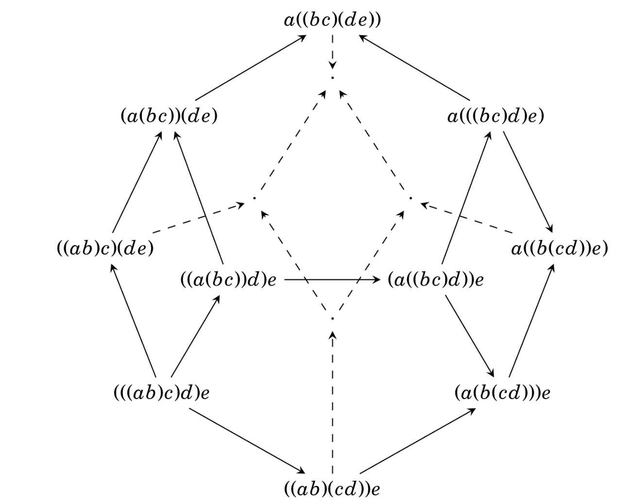
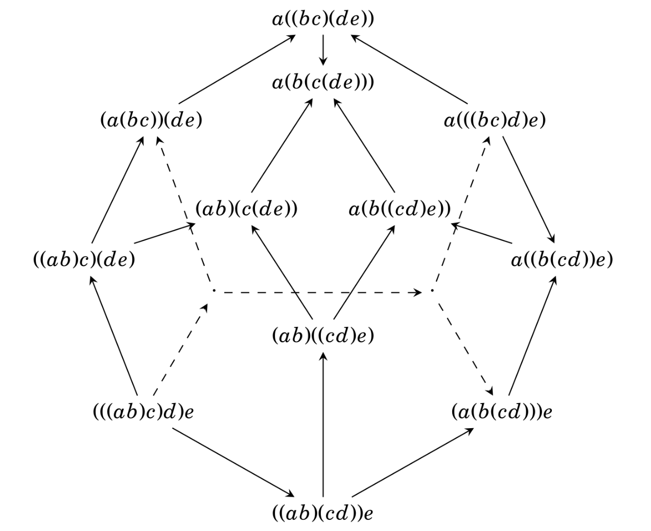
Figure 5. The Stasheff associahedron $K_{5}$, front and back view.

Boardman and Vogt [7] showed that the associahedron $K_{n}$ can be decomposed into $C_{n-1}$ cubes of dimension $n-2$, where $C_{n-1}$ is the Catalan number

$$C_{n-1}=\frac{1}{n}\binom{2n-2}{n-1}\,.$$

The decomposition of the associahedron $K_{4}$ is illustrated in Figure 6.

Each vertex of the associahedron can be identified with a planar binary rooted tree. A way to interpret the polytope points here is as metric structures on planar binary rooted trees that assign weights in ${\mathbb{R}}_{\geq}0$ to the internal edges of the tree, with degeneracies along the faces and vertices of the cubic decomposition, see Figure 6 for $K_{4}$. Each cube in the decomposition parameterizes the (normalized) choices of weights for the internal edges for the planar tree structure associated to that cube, and the faces are glued according to the transitions from one tree structure to an adjacent one, as dictated by the associahedron structure.

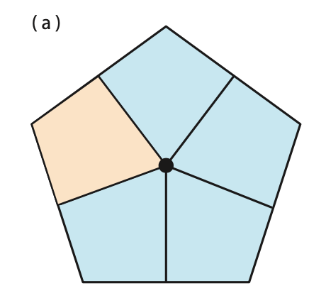
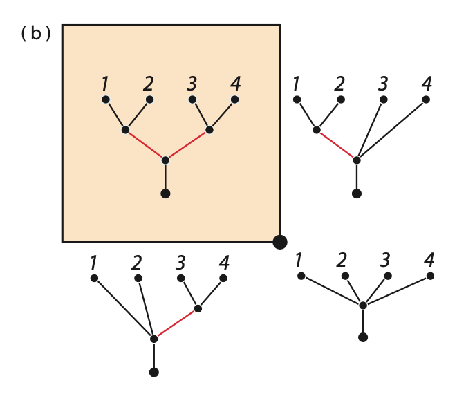
Figure 6. The Stasheff associahedron $K_{4}$ with its cubic decomposition (a), and parameterization of planar metric binary rooted trees (b), figures by Satyan Devadoss from [25].

It was further shown by Devadoss and Morava [25] that the parameterization of planar binary rooted trees with weights on the internal edges in terms of the (open cells of the) associahedron and its cubic decomposition can then be related to compactifications $\overline{M}_{0,n+1}({\mathbb{R}})$ of moduli spaces of real curves of genus zero with $(n+1)$-marked points. The key idea here is that the ordered leaves of a planar binary rooted trees can be embedded as an ordered set of points in the real line, where the coordinates of the points are obtained from the weights assigned at the internal edges of the tree as a function $e^{-W}$ of the sum $W$ of the weights along the path from the root to one of the leaves (see the example in Figure 7). Note that, while the open cells of the associahedron correspond to binary trees, the boundary strata of these cells contain trees with higher valences (corresponding to the limits of binary trees when one or more of the edge lengths go to zero). Since the trees coming from syntax are binary (see [61] for our discussion on why Merge operators with higher arity are excluded) the image from syntax will lie inside the open cells. The boundary structure is still important though, because boundaries of cells in the associahedron encode all the possible structural changes to the underlying hierarchical structures (syntactic objects).

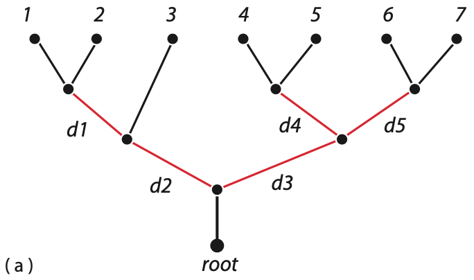
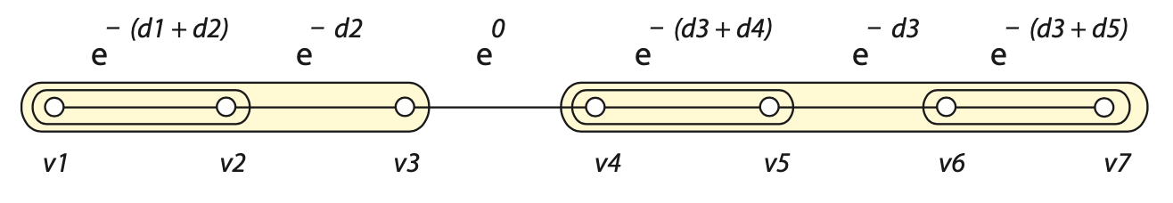
Figure 7. A planar binary rooted tree with weighted internal edges (a), and the associated ordered configuration of points on the real line, figures by Satyan Devadoss from [25].

As shown by Devadoss in [24], the orientation double cover $\overline{M}^{or}_{0,n+1}({\mathbb{R}})$ of $\overline{M}_{0,n+1}({\mathbb{R}})$ can be decomposed into a collection of $n!$ copies of the associahedron $K_{n}$, where the $n!/2$ associahedra of $\overline{M}_{0,n+1}({\mathbb{R}})$ correspond to the permutations of the $(n+1)$ points on the real line preserving the cyclic order of $\{0,1,\infty\}$, with gluings corresponding to certain twist operations on the triangulated $(n+1)$-gons (see Figure 10 for the example of $n=3$. Note that for $n\leq 3$, the moduli space $\overline{M}_{0,n+1}({\mathbb{R}})$ is orientable so one does not see the role of the orientation double cover; see [25] for a more detailed discussion of the more general case).

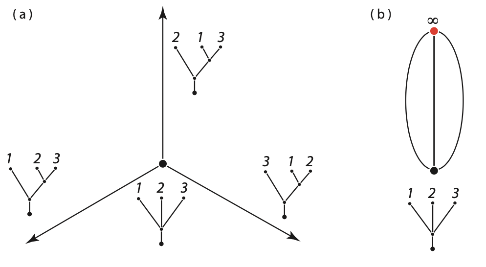
Figure 8. The moduli space ${\rm BHV}_{3}$ of abstract binary rooted trees and its one-point compactification ${\rm BHV}_{3}^{+}$, figure by Satyan Devadoss from [25].

One can also consider the moduli space ${\rm BHV}_{n}$ of abstract binary rooted trees with $n$ leaves (with no assigned planar structure) along with weighted internal edges, and their one-point compactification ${\rm BHV}^{+}$, constructed by Billera, Holmes, and Vogtmann, [5]. The moduli space ${\rm BHV}_{n}$ is obtained by considering all the $(2n-3)!!$ abstract binary rooted trees with $n$ labeled leaves. All these trees have $n-2$ internal edges. For each tree, one considers an orthant ${\mathbb{R}}_{\geq 0}^{n-2}$, which represents all the possible choices of a weight (length) for the internal edges. These orthants are glued along the common faces (which correspond to shrinking one of the internal edges) and this gives the space ${\rm BHV}_{n}$. The link ${\mathcal{L}}_{n}$ of the origin in ${\rm BHV}_{n}$ is an $(n-3)$-dimensional simplicial complex. In the case $n=3$ it consists of three points. For $n=4$ it is the Peterson graph of Figure 9. In general, there are $(2n-3)!!$ top $(n-3)$-dimensional simplexes of ${\mathcal{L}}_{n}$ (e.g. 15 edges in the case of ${\mathcal{L}}_{4}$) that correspond to the different trees, and two of them share a face when the corresponding trees give rise to the same quotient tree when contracting an internal edge.

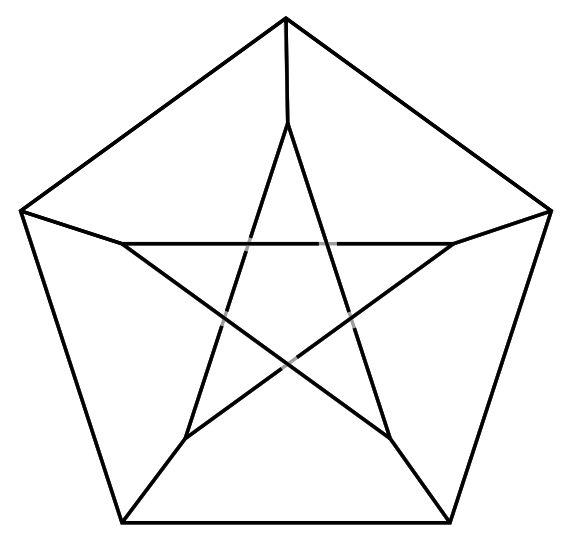
Figure 9. The Peterson graph is the link ${\mathcal{L}}_{4}$ of the origin in ${\rm BHV}_{4}$.

It is shown in [25] that there is a projection map between these moduli spaces,

(4.1) $$\Pi_{n}:\overline{M}^{or}_{0,n+1}({\mathbb{R}})\twoheadrightarrow{\rm BHV}_{n}^{+}\,,$$

with a finite projection that is generically $2^{n-1}$-to-$1$, obtained by an origami folding of the cubes of the cubical decomposition of the associahedra in $\overline{M}^{or}_{0,n+1}({\mathbb{R}})$, according to the formula

$$n!\cdot C_{n-1}=2^{n-1}\cdot(2n-3)!!\,,$$

where the left-hand-side lists the $C_{n-1}$ cubes of the $n!$ associahedra of $\overline{M}^{or}_{0,n+1}({\mathbb{R}})$, and the right-hand-side lists the $(2n-3)!!$ simplexes of dimension $(n-3)$ of ${\mathcal{L}}_{n}$, and $2^{n-1}$ is the multiplicity of the generic fibers of the projection map. Note that $2^{n-1}$ is the number of different planar structures for a given abstract binary rooted tree on $n$ leaves, since such a tree has $n-1$ non-leaf vertices and the total number of planar embeddings can be obtained by choosing one of two possible planar embeddings (left/right) for each pair of edges below a given non-leaf vertex. The origami folding quotient takes each $(n-2)$-dimensional cube and folds it in half in each direction, obtaining $2^{n-2}$ foldings, with $2$ copies of each cube in the orientation double cover, so that one obtains $2^{n-1}$ points in each general fiber. We will see this more explicitly in §4.3, applied to our setting.

4.3. Head functions, convex semantic spaces, and metric trees

With these facts in hand, now consider again the setting we discussed in our simple example of §2.2.3.

Consider the set of all $(2n-3)!!$ abstract binary rooted trees with $n$ labeled leaves. Suppose that the leaves are labeled by a given (multi)set $\{\lambda_{i}\}_{i=1}^{n}$ of lexical items and syntactic features in ${\mathcal{S}}{\mathcal{O}}_{0}$. If this is a multiset instead of a set, we still interpret the multiple copies of a given item in ${\mathcal{S}}{\mathcal{O}}_{0}$ as repetitions, not as copies, in the sense that they can play different roles in structure formation via applications of Merge–hence we will still regard them as distinct labels. Thus, we have the following geometric description of our data.

• For any choice of the lexical items associated to the leaves, we obtain a corresponding copy of the moduli space ${\rm BHV}_{n}$.

• The link of the origin ${\mathcal{L}}_{n}\subset{\rm BHV}_{n}$ can be seen as an assignment of weights to the internal edges that is normalized (for example by requiring that the total sum of weights is equal to $1$).

• We write ${\rm BHV}_{n}(\Lambda)$ for $\Lambda=\{\lambda_{i}\}_{i=1}^{n}$ for the copy of ${\rm BHV}_{n}$ that corresponds to the given choice $\Lambda$ of the lexical items assigned to the leaves.

• We similarly write ${\mathcal{L}}_{n}(\Lambda)$ for the associated copy of ${\mathcal{L}}_{n}$.

Proposition 4.1.

The choice of a head function $h$ determines simplicial subcomplexes ${\mathcal{L}}_{n}(\Lambda,h)\subset{\mathcal{L}}_{n}(\Lambda)$, ${\rm BHV}_{n}(\Lambda,h)\subset{\rm BHV}_{n}(\Lambda)$, $M_{n}(\Lambda,h)\subset\overline{M}^{or}_{0,n+1}({\mathbb{R}})$, compatible with the maps relating these moduli spaces, and a lift of ${\mathcal{L}}_{n}(\Lambda,h)$ and ${\rm BHV}_{n}(\Lambda,h)$ inside $M_{n}(\Lambda,h)$, determined by the planar structure $\pi_{h}$ associated to the head function.

Proof.

The choice of the head function $h$ selects, for each of these copies ${\mathcal{L}}_{n}(\Lambda)\subset{\rm BHV}_{n}(\Lambda)$, a simplicial subcomplex ${\mathcal{L}}_{n}(\Lambda,h)\subset{\mathcal{L}}_{n}(\Lambda)$ and the associated cone ${\rm BHV}_{n}(\Lambda,h)\subset{\rm BHV}_{n}(\Lambda)$, where the set of top $(n-3)$-dimensional simplexes of ${\mathcal{L}}_{n}(\Lambda,h)$ corresponds to the subset of the given $(2n-3)!!$ trees that belong to ${\rm Dom}(h)$.

Let $M_{n}(\Lambda,h)\subset\overline{M}^{or}_{0,n+1}({\mathbb{R}})$ denote the locus in $\overline{M}^{or}_{0,n+1}({\mathbb{R}})$ obtained as a pre-image under the projection map of the image ${\rm BHV}_{n}(\Lambda,h)^{+}$ of the cone ${\rm BHV}_{n}(\Lambda,h)$ in the one-point compactification ${\rm BHV}_{n}^{+}$,

(4.2) $$M_{n}(\Lambda,h):=\Pi_{n}^{-1}({\rm BHV}_{n}(\Lambda,h)^{+})\,.$$

A point in ${\rm BHV}_{n}(\Lambda,h)$ is a pair $(T,\underline{\ell})$ of an abstract binary rooted tree on $n$ leaves labeled by the points of $\Lambda$ together with a set $\underline{\ell}=(\ell_{k})_{k=1}^{n-2}$ of weights $\ell_{i}\in{\mathbb{R}}_{\geq 0}$ assigned to the internal edges of $T$. The $2^{n-1}$ points in the fiber $\Pi_{n}^{-1}(T,\underline{\ell})\subset M_{n}(\Lambda,h)$ are given by the points $(T^{\pi},\underline{\ell})$, where $T^{\pi}$ ranges over all the possible planarizations $\pi$ of $T$ and the lengths of the internal edges stay the same.

We have seen that the choice of a head function $h$ determines an associated planar structure $\pi_{h}$ for all trees $T\in{\rm Dom}(h)$. Thus, the choice of a head function determines a lift of the subcomplex ${\rm BHV}_{n}(\Lambda,h)$ (and in particular of ${\mathcal{L}}_{n}(\Lambda,h)\subset{\mathcal{L}}_{n}(\Lambda)$) to a subcomplex of $M_{n}(\Lambda,h)\subset\overline{M}^{or}_{0,n+1}({\mathbb{R}})$. ∎

Consider then, as in §2.2.3, a semantic space ${\mathcal{S}}$ that is a geodesically convex subspace of a Riemannian manifold, together with a map $s:{\mathcal{S}}{\mathcal{O}}_{0}\to{\mathcal{S}}$. Assume that, for points in ${\mathcal{S}}$, we can evaluate the frequency of semantic relatedness in a specified context in terms of a biconcave function ${\mathbb{P}}:{\rm Sym}^{2}({\mathcal{S}})\to[0,1]$.

Proposition 4.2.

Let $T\in{\rm Dom}(h)\subset{\mathfrak{T}}_{{\mathcal{S}}{\mathcal{O}}_{0}}$ be a tree with $n$ leaves. The data $(s:{\mathcal{S}}{\mathcal{O}}_{0}\to{\mathcal{S}},{\mathbb{P}})$ determine a set $\underline{\ell}=(\ell_{k})_{k=1}^{n-2}\in{\mathbb{R}}^{n-2}_{\geq 0}$ of weights assigned to the internal edges of $T$. Thus the data $(s:{\mathcal{S}}{\mathcal{O}}_{0}\to{\mathcal{S}},{\mathbb{P}})$ determine a point $(T,\underline{\ell}^{(h,s,{\mathbb{P}})})\in{\mathcal{L}}_{n}(\Lambda,h)$ and a point in the corresponding fiber of the projection from $M_{n}(\Lambda,h)$.

Proof.

To see this, we proceed as in §2.2.3. For each of the $n-2$ vertices $v$ of $T$ that are neither the root nor one of the leaves, consider the two subtrees $T_{v,1}$ and $T_{v_{2}}$ that have root vertices $v_{1},v_{2}$ immediately below $v$, and compute $p_{v}:={\mathbb{P}}(s(T_{v,1}),s(T_{v,2}))$, where $h(T_{v,i})$ is the head leaf of the subtree $T_{v,i}$. We label the $(n-2)$ internal edges by the target vertex $v$ (where the tree is oriented away from the root) and we take $\ell_{v}=p_{v}$.

Thus, we have that, for a tree $T\in{\rm Dom}(h)\subset{\mathfrak{T}}_{{\mathcal{S}}{\mathcal{O}}_{0}}$ on $n$ leaves labeled by $\Lambda$, the choice of a head function $h$, together with the choice of a map $s:{\mathcal{S}}{\mathcal{O}}_{0}\to{\mathcal{S}}$ and of the function ${\mathbb{P}}:{\rm Sym}^{2}({\mathcal{S}})\to[0,1]$ determines, after an overall normalization of the weights, a point $(T,\underline{\ell}^{(h,s,{\mathbb{P}})})\in{\mathcal{L}}_{n}(\Lambda,h)$, and a corresponding point $(T^{\pi_{h}},\underline{\ell}^{(h,s,{\mathbb{P}})})\in{\mathcal{L}}_{n}(\Lambda,h)$ in the fiber above $(T,\underline{\ell}^{(h,s,{\mathbb{P}})})$ in $M_{n}(\Lambda,h)\subset\overline{M}^{or}_{0,n+1}({\mathbb{R}})$. ∎

Remark 4.1.

Note that in §2.2.3 we used the same coordinates ${\mathbb{P}}(s(T_{v,1}),s(T_{v,2}))$ to assign points $s(T_{v})=p_{v}s(T_{v,1})+(1-p_{v})s(T_{v,2})$ or $s(T_{v})=p_{v}s(T_{v,2})+(1-p_{v})s(T_{v,1})$ (according to whether the head $h(T_{v})$ matches the head of either of the two subtrees). Thus, according to this construction, the weight of an internal edges of $T$ obtained as in Proposition 4.2 reflects the positions in the semantic space ${\mathcal{S}}$ of the accessible term below that edge.

As a result, we can view the construction of the character $\phi_{s,{\mathbb{P}},h}$ of §2.2.3 equivalently as the construction of a section.

Corollary 4.2.

The construction of the character $\phi_{s,{\mathbb{P}},h}$ of §2.2.3 is equivalent to the construction of a partially defined section

(4.3) $$\sigma_{s,{\mathbb{P}},h,n}:{\rm BHV}_{n}\to\overline{M}^{or}_{0,n+1}({\mathbb{R}})$$

which is defined over

$${\rm Dom}(\sigma_{s,{\mathbb{P}},h,n})={\rm BHV}_{n}(\Lambda,h)\,,$$

and a partially defined map

(4.4) $$s_{{\mathbb{P}},h}:{\mathfrak{T}}_{{\mathcal{S}}{\mathcal{O}}_{0}}\to\cup_{n}{\mathcal{L}}_{n}(\Lambda,h)$$

with ${\rm Dom}(s_{{\mathbb{P}},h})={\rm Dom}(h)$. The construction of the character $\phi_{s,{\mathbb{P}},h}$ of §2.2.3 is equivalent to the construction of the composite map $\sigma_{s,{\mathbb{P}},h}\circ s_{{\mathbb{P}},h}$.

For the case $n=3$, the projection maps are illustrated in Figure 10.

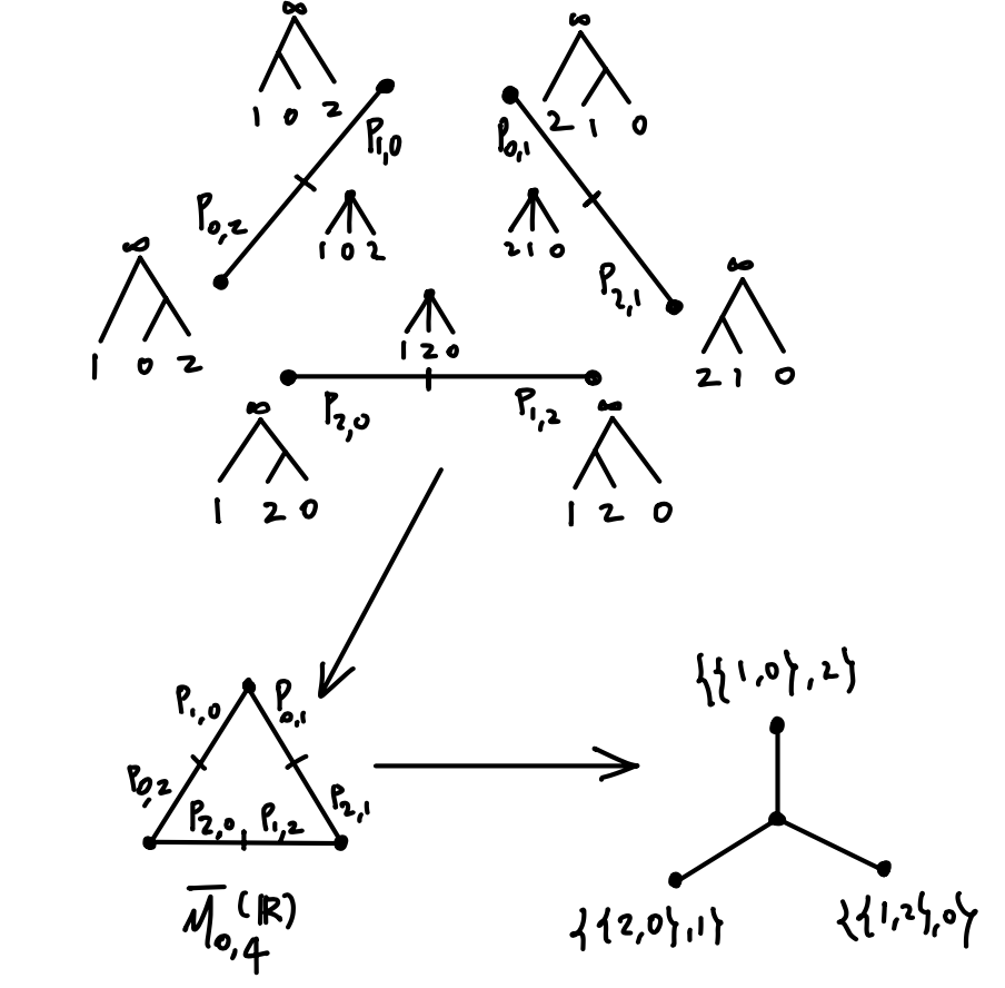
Figure 10. The projections from three associahedra $K_{3}$ to the moduli space $\overline{M}_{0,4}({\mathbb{R}})$ and to the ${\rm BHV}_{3}^{+}$ moduli space and the embedding map ${\mathcal{I}}$ of syntactic trees to semantic space ${\mathcal{S}}$ seen from the point of view of moduli spaces.

We have described the construction here in terms of the simple model of assignment of semantic values to syntactic objects described in §2.2.3. This can be adapted to other models, so that we can incorporate, as part of the modeling of the syntax-semantics interface, the construction of a partially defined section

(4.5) $$\sigma_{{\mathcal{S}},n}:{\rm Dom}(\sigma_{\mathcal{S}})\subset{\rm BHV}_{n}\to\overline{M}^{or}_{0,n+1}({\mathbb{R}})$$

which depends on the model of semantic space ${\mathcal{S}}$ used and on its properties. Similarly, the map (4.4) can be generalized as a map

(4.6) $$s_{{\mathcal{S}},h,n}:{\mathfrak{T}}_{{\mathcal{S}}{\mathcal{O}}_{0}}\to{\mathcal{L}}_{n}\cap{\rm Dom}(\sigma_{{\mathcal{S}},n})\,.$$

4.4. Origami folding and Externalization

In [61] we gave an account of Externalization as a section of the projection from planar to abstract binary rooted trees, where the section is language dependent and is chosen so that the resulting planar structure is compatible with certain syntactic parameters, through the effect these have on word order.

In terms of the geometry of moduli spaces described here, one can similarly view Externalization as the choice of a section (depending on a specified language $L$ through its syntactic parameters)

(4.7) $$\sigma_{L,n}:{\rm BHV}_{n}\to\overline{M}^{or}_{0,n+1}({\mathbb{R}})\,.$$

This section is defined at the level of the combinatorial trees, as a choice of a section $\sigma_{L,n}:{\mathfrak{T}}_{{\mathcal{S}}{\mathcal{O}}_{0},n}\to{\mathfrak{T}}_{{\mathcal{S}}{\mathcal{O}}_{0},n}^{pl}$ that assigns a planar structure, as discussed in [61], and extended to metric trees as the identity on the metric datum $\underline{\ell}$, since Externalization is decoupled from the metric structure, reflecting our initial assumption on independence of semantic values from Externalization. This independence assumption only affects this independence of $\sigma_{L,n}$ on the metric structure. It does not mean that there would be no interaction with the semantics channel. One way to model such interaction is by comparing the two sections $\sigma_{L,n}$ and $\sigma_{{\mathcal{S}},n}$ on the subdomain ${\rm Dom}(\sigma_{{\mathcal{S}},n})\subset{\rm BHV}_{n}$ where both are defined and in particular on the target of the map $s_{{\mathcal{S}},h,n}$ of (4.6).

4.5. An example

All the above discussion on the relation between Externalization and the syntax-semantics interface in terms of moduli spaces is quite abstract, so let us illustrate what is happening with a very simple example. Consider a sentence such as

$$\Tree[[yellowflowers][bloomearly]]=\Tree[[\alpha\beta][\gamma\delta]]=((\alpha\,\,\beta)\,(\gamma\,\,\delta))$$

In the form depicted, this is represented by a planar binary rooted tree on four leaves labeled by the lexical items in the set $\Lambda=\{\alpha,\beta,\gamma,\delta\}$. The tree does not contain exocentric constructions and has a well defined syntactic head. Thus, we have the associated data $(\Lambda,h)$ as above. The underlying syntactic object, as produced by a free symmetric Merge. is the non-planar abstract binary rooted tree

$$\Tree[[\alpha\beta][\gamma\delta]]=\Tree[[\beta\alpha][\gamma\delta]]=\Tree[[\alpha\beta][\delta\gamma]]=\Tree[[\gamma\delta][\alpha\beta]]=\{\{\alpha,\beta\},\{\gamma,\delta\}\}\,.$$

The planar tree $((\alpha\,\,\beta)\,(\gamma\,\,\delta))$ corresponds to a vertex of the associahedron $K_{4}$, as in Figure 11. The associahedron considered is one of the $4!=24$ associahedra that correspond to the $4!$ permutations of the leaves’ labels. This assignment of a vertex on one of the $24$ associahedra corresponds to left arrow (free symmetric Merge to Externalization) in the top part of Figure 4, for this example.

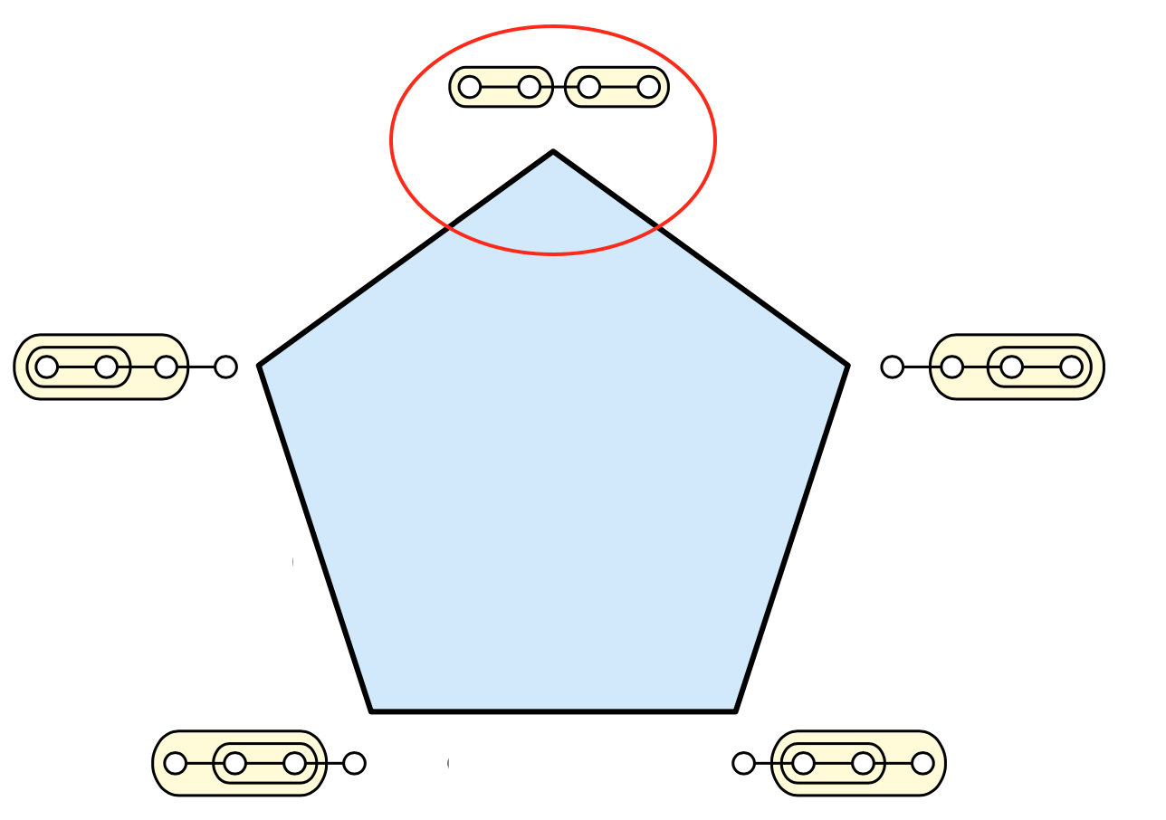
Figure 11. The selected vertex of the associahedron $K_{4}$ corresponding to the planar tree $((\alpha\,\,\beta)\,(\gamma\,\,\delta))$ (modified figure by Satyan Devadoss from [25]).

The abstract tree $\{\{\alpha,\beta\},\{\gamma,\delta\}\}$ produced by the free symmetric Merge, on the other hand, is one of the $15=(2n-3)!!$, for $n=4$, possible abstract binary rooted trees on four labeled leaves. These $15$ possible trees correspond to the $15$ edges of the link ${\mathcal{L}}_{4}$ of the origin in the moduli space $BHV_{4}$. Thus, the syntactic object $\{\{\alpha,\beta\},\{\gamma,\delta\}\}$ selects one of these edges, see Figure 12.

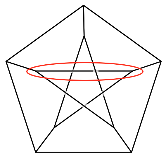
Figure 12. The selected edge in the link ${\mathcal{L}}_{4}$ of the origin in the moduli space BHV₄ corresponding to the abstract tree $\{\{\alpha,\beta\},\{\gamma,\delta\}\}$.

Now suppose we have chosen a semantic space ${\mathcal{S}}$ (for simplicity of discussion, consider using a vector space model, though it is not necessary for ${\mathcal{S}}$ to be of this kind). Each of the four lexical items has a representation $s(\alpha),s(\beta),s(\gamma),s(\delta)\in{\mathcal{S}}$. The two semantic relatedness measures $u_{1}={\mathbb{P}}(s(\alpha),s(\beta))$ (relating “yellow” and “flower”) and $u_{2}={\mathbb{P}}(s(\gamma),s(\delta))$ (relating “blooming” and “early”) in ${\mathcal{S}}$ provide two real coordinates associated with the accessible terms $\{\alpha,\beta\}$ and $\{\gamma,\delta\}$, respectively. These two coordinates fix a point $(u_{1},u_{2})\in[0,1]^{2}$ in a square (see Figure 13). The selected edge of Figure 12 corresponds to the diagonal of the square given by $u_{1}+u_{2}=1$. Thus, the mapping of the result of the free symmetric Merge to semantic space determines a point in the moduli space $BHV_{4}^{+}$. This completes the right arrow (free symmetric Merge to Semantic Spaces) in the top part of Figure 4, for the example of this simple sentence.

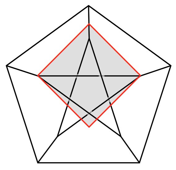
Figure 13. The square and the selected edge in the link ${\mathcal{L}}_{4}$ for corresponding to the abstract tree $T=\{\{\alpha,\beta\},\{\gamma,\delta\}\}$: the mapping of $T$ to semantic space selects a point in this square.

We next see in this example the bottom part of Figure 4, that describes the compatibility between Externalization and the syntax-semantics interface. First note that the associahedra $K_{4}$ are tiled with squares (quadrangles), as in Figure 14. The two vertices of the square adjacent to the marked vertex of the pentagon corresponds to degenerate trees where one or the other of the internal edges as shrunk to zero length, while the other has normalized length one. Thus, we see that we can map this square to the square of Figure 13 through the same coordinates $(u_{1},u_{2})$ describing the lengths of the two internal edges (compare with Figure 10 for the case $n=3$).

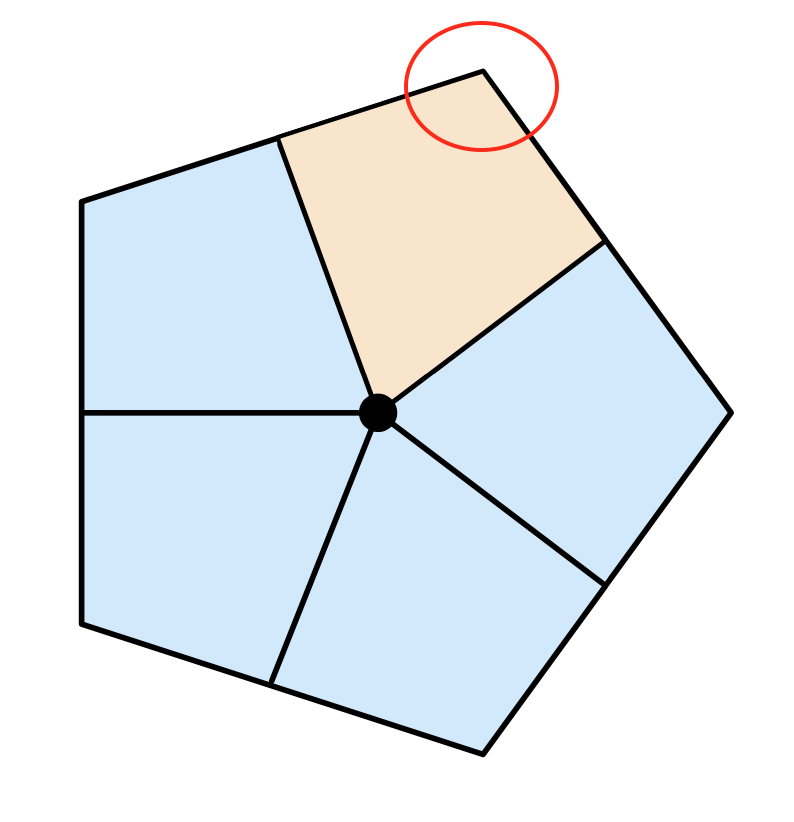
Figure 14. The associahedron $K_{4}$ tiled with squares (quadrangles), with the selected vertex associated to $((\alpha\,\,\beta)\,(\gamma\,\,\delta))$ (modified figure by Satyan Devadoss from [25]).

This lifting of the point associated to $T$ in the square of Figure 13 to a corresponding point in the square of Figure 13 is the effect of the section $\sigma_{L,4}$ described in (4.7). To see this, we need to take into consideration the fact that the $24$ associahedra combine together into a single geometric space, obtained by gluing them along their boundaries. This is done in two steps: first $12$ associahedra are glued along their boundaries as in the left-hand-side of Figure 15, forming the space $\bar{M}_{0,5}({\mathbb{R}})$. Then the orientation double cover is formed: in a self-intersecting $3$-dimensional visualization, this resulting space $\bar{M}^{or}_{0,5}({\mathbb{R}})$ can be identified with the great dodecahedron in the right-hand-side of Figure 15. It is not easy to see from its $3D$ representation as great dodecahedron, but the space $\bar{M}^{or}_{0,5}({\mathbb{R}})$ is a genus $4$ hyperbolic surface, and can be seen more directly from its description in terms of fundamental domain given in [1], as in Figure 16 below.

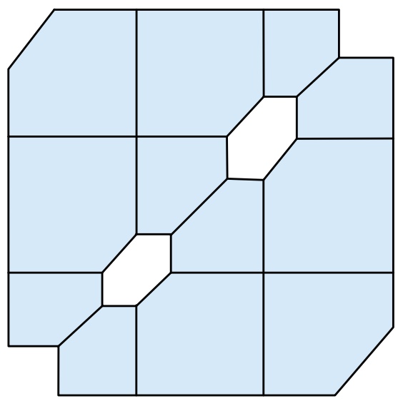
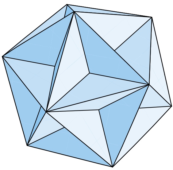
Figure 15. Twelve associahedra $K_{4}$ assemble into the space $\bar{M}_{0,5}({\mathbb{R}})$ and its orientation double cover gives $24$ associahedra assembled into the space $\bar{M}^{or}_{0,5}({\mathbb{R}})$ identified with the great dodecahedron (figure by Satyan Devadoss from [25]).

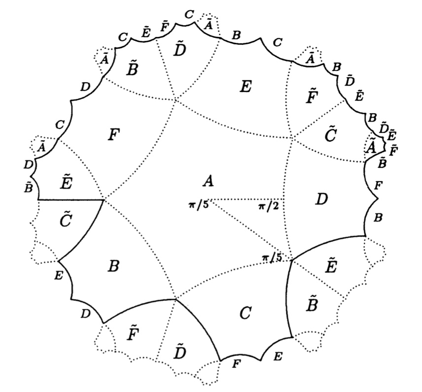
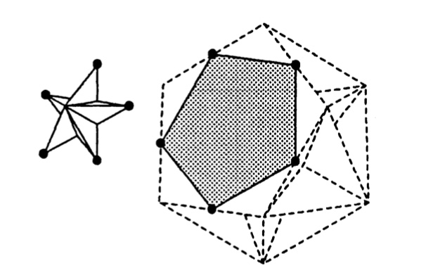
Figure 16. The great dodecahedron $\bar{M}^{or}_{0,5}({\mathbb{R}})$ as a hyperbolic genus $4$ surface, and the two different forms of the $24$ associahedron tiles (figure from [1]).

The projection map $\Pi_{4}:\overline{M}^{or}_{0,5}({\mathbb{R}})\twoheadrightarrow{\rm BHV}_{4}^{+}$ of (4.1) folds together and identifies $8$ squares in $\overline{M}^{or}_{0,5}({\mathbb{R}})$ to each square in ${\rm BHV}_{4}^{+}$. Thus, when we lift to $\overline{M}^{or}_{0,5}({\mathbb{R}})$ the point assigned to the tree $T$ in one of the squares of ${\rm BHV}_{4}^{+}$ by the mapping of $T$ to semantic space, the lifted point lies on one of the $8$ preimages of the given square of ${\rm BHV}_{4}^{+}$. This choice of one ut of the $8$ preimages is the choice of planar structure of the syntactic object determined by externalization and this gives indeed the section $\sigma_{L,4}$ described in (4.7), where here $L=\,$English.

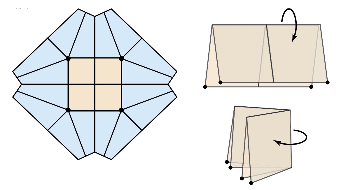
Figure 17. Four squares in adjacent associahedra $K_{4}$ are folded together (origami folding) in the projection to ${\rm BHV}_{4}^{+}$ so that $8$ squares in the double cover $\overline{M}^{or}_{0,5}({\mathbb{R}})$ are identified in the projection $\Pi_{4}:\overline{M}^{or}_{0,5}({\mathbb{R}})\twoheadrightarrow{\rm BHV}_{4}^{+}$ (figure by Satyan Devadoss from [25]).

One can then see in this same simple example, that if instead of taking the planarization $T^{\pi_{L}}=((\alpha\,\,\beta)\,(\gamma\,\,\delta))$ of the syntactic object $T=\{\{\alpha,\beta\},\,\{\gamma,\delta\}\}$, one would take the planarization $T^{\pi_{h}}$ determined by the head function, one would end up with the different planar tree

$$T^{\pi_{h}}=\Tree[[\gamma\delta][\beta\alpha]]=((\gamma\delta)(\beta\alpha))\,.$$

This means that one ends up on a different one of the $24$ associahedra and a square inside that associahedron, that is still one of the $8$ squares that project to the same (unchanged) square in ${\rm BHV}_{4}^{+}$. The same point in this square in ${\rm BHV}_{4}^{+}$ determined by mapping $T$ to semantic space is then lifted to a corresponding point in a different square inside $\overline{M}^{or}_{0,5}({\mathbb{R}})$. This means that we are considering a different section of the projection $\Pi_{4}$. This is the section $\sigma_{{\mathcal{S}},4}$ described in (4.5). The difference between these two sections is measured by a transformation $\gamma_{L,4}\circ\sigma_{L,4}=\sigma_{{\mathcal{S}},4}$, where applied to our syntactic object $T$ this gives the permutation $\gamma_{L,4}(T)=(3421)$. As in (4.8), this transformation $\gamma_{L,4}$ is Kayne’s LCA algorithm for this very simple example.

We have considered a very simple example with $n=4$ where the geometry is straightforward to visualize. The spaces $\overline{M}^{or}_{0,n+1}({\mathbb{R}})$ and ${\rm BHV}_{n}^{+}$ grow significantly in combinatorial complexity as $n$ becomes larger, but they are still very well understood and widely studied geometric spaces. Other more complicated geometries are likely to arise if the mapping of syntactic objects to semantic spaces is done in a more sophisticated and informative way than the very simple type of mappings we considered in this paper as illustrative examples.

4.6. Geometric view of some planarization questions

We conclude this section by briefly commenting on how certain frameworks where the question of planarization of syntactic objects arises can be also seen in terms of the geometry described above. We discuss briefly Kayne’s Linear Correspondence Axiom and Cinque’s Abstract Functional Lexicon, and we also outline how one can describe the role of syntactic parameters in this geometric setting.

4.6.1. Kayne’s LCA algorithm

When the planar structure assigned by the section $\sigma_{{\mathcal{S}},n}$ is the planar structure $\pi_{h}$ determined by a head function, as in the case of (4.3), this means comparing the planar structure $\pi_{h}$, for $h$ defined on ${\rm Dom}(h)\subset{\mathfrak{T}}_{{\mathcal{S}}{\mathcal{O}}_{0}}$, with the planar structure $\pi_{L}$ defined by the section $\sigma_{L,n}$ through the constraints imposed by the syntactic parameters of the language $L$. This comparison can be seen as a version of Richard Kayne’s LCA (Linear Correspondence Axiom), [48], [49]. As we observed in [62], Kayne’s LCA cannot be defined globally on ${\mathfrak{T}}_{{\mathcal{S}}{\mathcal{O}}_{0}}$, but is only partially defined on the domain ${\rm Dom}(h)$ of a head function (the syntactic head), hence it does not play the same role as Externalization, which is a choice of a globally defined (non-canonical) section $\sigma_{L,n}$. However, on the domain ${\rm Range}(s_{{\mathcal{S}},h,n})\subset{\mathcal{L}}_{n}\cap{\rm Dom}(h)$ where both $\sigma_{L,n}$ and $\sigma_{{\mathcal{S}},n}$ are defined there exists a covering transformation $\gamma_{L,n}$ of the projection map

$$\overline{M}^{or}_{0,n+1}({\mathbb{R}})\to{\rm BHV}_{n}^{+}$$

that satisfies

(4.8) $$\gamma_{L,n}\circ\sigma_{L,n}=\sigma_{{\mathcal{S}},n}$$

at all points in ${\rm Range}(s_{{\mathcal{S}},h,n})$. This covering transformation $\gamma_{L,n}$ plays the role of the (partially defined) LCA algorithm.

4.6.2. Cinque’s abstract functional lexicon

There are other constructions that one can fit into this geometric picture with the projection map $\overline{M}^{or}_{0,n+1}({\mathbb{R}})\to{\rm BHV}_{n}^{+}$–partially defined sections, and covering transformations permuting the $2^{n-1}$ points of the fibers of the projection map. For example, one can view this as the abstract functional lexicon described by Cinque [19].

In [19], Cinque considers the problem of comparing word order relations imposed on individual languages by particular syntactic parameters, with a certain base ordering relation of proximity to the verbal properties of different morphemes (in a structural sense, rather than in terms of linear ordering), such as mood, tense, modality aspect, and voice. In [19], a general hierarchy of functional morphemes and of adverbial classes is identified (see (6) and (7) of [19]). As observed in [19], with verbal morphemes as heads and corresponding classes of adverbs as phrases in so-called specifier position, this hierarchy determines a planar embedding (in the way that it appears in (6) and (7) of [19]). Syntactic parameters, on the other hand, also determine a planar embedding. While this could be a priori arbitrary, the variability across languages is far less than the space of combinatorial possibilities would allow. Also, different word order constraints appear not to be independent, but to exhibit a significant degree of relatedness. This can be seen both at the theoretical level (see [37]) and at the level of database analysis of syntactic parameters (see [70], [72], [75]).

In terms of the geometry of moduli spaces described above, one can describe the difference between the ordering (planar structure) described by Cinque in [19] and the deviation from it in the word order of specific languages in terms of covering tranformations $\gamma_{L,n}$ of the projection map $\overline{M}^{or}_{0,n+1}({\mathbb{R}})\to{\rm BHV}_{n}^{+}$ that act as permutations of the planar structures, and are language specific. The degree to which word order constraints deviate from the base structural hierarchy described in Cinque can then be measured in terms of how far the $\gamma_{L,n}$ are from the identity in the group of covering transformations of the projection map.

4.6.3. A geometric view of syntactic parameters

Syntactic parameters fix constraints on the planar structure of Externalization. For an extensive recent account of syntactic parameters see [77]. In [61] we interpreted the role of syntactic parameters as constraints on the choice of a language-dependent section $\sigma_{L,n}$ for the Externalization of free symmetric Merge.

The discussion above shows that in our setting we can also interpret the role of syntactic parameters in a geometric way, as the choice, for a given language $L$, of a collection $L\mapsto\{\gamma_{L,n}\}_{n}$ of covering transformations of the projections $\overline{M}^{or}_{0,n+1}({\mathbb{R}})\to{\rm BHV}_{n}^{+}$, as in (4.8). Comparison of syntactic parameters across languages can be formulated in various computational forms. This includes the difficult problem of understanding the relation among parameters, as well as the much lower dimensional space occupied by actual languages inside the high-dimensional space of possible values of the hundreds of parameters currently studied (see for example [41], [53], [59], [50], [75], [80]). In particular, one can focus on the effect of syntactic parameters on word order constraints. In this case, using the framework we consider here, one can view this comparison across languages as the comparison between sections $\sigma_{L,n}$ for different languages $L$, or equivalently as the properties of the collection of elements $\gamma_{L,n}\gamma_{L^{\prime},n}^{-1}$, for $L\neq L^{\prime}$ in the group of covering transformations of $\overline{M}^{or}_{0,n+1}({\mathbb{R}})\to{\rm BHV}_{n}^{+}$.

5. Birkhoff factorization and (semi)ring parsing

We now extend the setting introduced above to more refined descriptions of the characters and factorization, that incorporate more detailed properties of semantic parsing and compositionality. We first focus on semiring parsing, as in [36], while in §6 we analyze how our model relates to Pietroski’s theory of minimalist meaning, [73]. These two settings represent very different models, where semiring semantics incorporates the idea of truth-values and generalizes it to values in arbitrary (semi)rings, not necessarily Boolean, while Pietroski’s approach provides an alternative that bypasses the idea of truth-values entirely and is based on a compositional structure modeled on the Minimalism’s Merge operation.

In this section we analyze (semi)ring parsing, introducing a version that is adapted to Minimalism formulated in terms of free symmetric Merge.

Since this is the most mathematically-heavy section in this paper, we provide a preliminary outline of the content and a more heuristic explanation of what is covered in the various subsections, before starting to discuss the more precise details.

5.1. Preliminary discussion

The relation between grammars and semirings was first observed by Chomsky–Schützenberger in [17]. Semiring parsing (see for instance [36]), when formulated in the setting of context-free grammars, considers deduction rules of the form

$$\frac{A_{1}\ldots A_{k}}{B}C_{1}\ldots C_{\ell}\,,$$

where the terms $A_{i}$ (main conditions) are rules $R$ of the grammar or input nonterminals and the $C_{i}$ are (non-probabilistic) Boolean side conditions and the fraction notation means that if the numerator terms hold then the denominator term also does. To the main condition terms one assigns values in a semiring, combined with the semiring operations, to obtain a value for the deduced output. The target semiring varies according to the parsing algorithm considered. The main choices include the Boolean semiring, the tropical semiring, the probability semiring (that is, the familiar case of Viterbi parsing), as well as the non-commutative derivation forest semiring, that collects all the possible derivations, with concatenation as multiplication and union as semiring addition. Often, parsing with values in other semirings factor through the derivations semiring. This setting is specifically constructed in the formal language context, and specifically for context-free grammars, though some generalizations exist in mildly context-sensitive classes like those produced by tree-adjoining grammars (TAGs).

A natural question arises about what type of algebraic structure replaces this form of semiring parsing in the setting of Minimalism, and more specifically the form of Minimalism based on free symmetric Merge.

The main goal of this section is to provide an answer to this question, in a form that is again based on the Birkhoff factorization procedure, that we present throughout this paper as a natural formalism for different forms of assignments of semantic values in the context of a free symmetric Merge model of syntax.

Developing this form of “semiring parsing” (where semirings will in fact be replaced by more general algebraic objects) requires several steps, that we now briefly summarize.

In §5.2 we introduce a ring of Merge derivations, formed by considering chains of Merge operations, given by the action of Merge on workspaces. These are assembled into a ring structure, where the linear structure is obtained by taking the vector space spanned by the derivations (that is, including formal linear combinations) and the multiplication operation is the union of the workspaces with the corresponding Merge actions. These are the same operations on the algebra part of the Hopf algebra of workspaces that we introduced in [61] and used earlier in this paper. We only consider the product structure on this ring and not the coproduct, as we have on the Hopf algebra of workspaces. However, this does not lead to a loss of structure in this case, because the coproduct is built into the Merge operation on workspaces, so it it still encoded into the data of this ring of Merge derivations.

In order to illustrate more clearly the properties of this ring of Merge derivations, in §5.2 we return to discuss the notion of Minimal Search in the Merge model of syntax. In [61] we gave an account of how Minimal Search is implemented as extraction of leading order term in the action of Merge on workspaces. This leading order term contains Internal and External Merge, while it excludes other presumptively unwanted forms of Merge (Sideward and Countercyclic). The idea of extraction of the leading order term is closely related to Birkhoff factorization, as originally observed in the context of the renormalization in physics.

Here we show that in fact, after extending the ring of Merge derivations to a ring of Laurent series with coefficients in this ring, one can indeed show that Minimal Search is exactly a Birkhoff factorization in this ring–for a character from the Hopf algebra of workspaces that assigns to a workspace its Merge derivation and a power that counts the effect of that derivation on the size of the workspace. The Birkhoff factorization separates out, on one side, the unwanted forms of Merge, while retaining on the other side only fundamental ones, namely External and Internal Merge. This case of Birkhoff factorization happens to be the one that is closest to the original form used in physics.

This result on Minimal Search as Birkhoff factorization in §5.2 is not required for the following parts of this section, and is included to provide some more direct understanding of the ring of Merge derivations and to connect it to our original formulation in [61]. This section can be skipped (except for Definition 5.1) by the readers interested in directly accessing the discussion of how to extend the semiring parsing framework.

The main construction for the generalization of semiring parsing starts in §5.3. The main viewpoint here is that, in order to formulate semiring parsing for Merge derivations based on the action of Merge on workspaces, one needs to replace the setting of Hopf algebras and semirings, that we used in the previous sections of this paper to describe simple models of syntax-semantics interface, with a slightly more flexible form, where the algebraic structures of Hopf algebra and semiring are replaced by their “categorified” form, which we refer to, respectively, as Hopf algebroids and semiringoids. The reason for this extension is very simple. Merge derivations given by actions of Merge on workspaces only compose when the target workspace of one derivation agrees with the source workspace of the next. This differs from the situation we considered in the previous sections where we only considered the Hopf algebra of workspaces, where the product is the disjoint union (combination of workspaces) which is always defined without source/target matching conditions.

Thus, just as in passing from the multiplication in a group to the multiplication in a groupoid, that precisely accounts for the fact that arrows compose only when the target of the first is the source of the second, one can obtain similar generalizations of the structures of Hopf algebra and Rota–Baxter algebra (or semiring) that we used in the formulation of mapping from syntax to semantics as Birkhoff factorization in the previous sections.

An extension of the notion of Hopf algebra that accommodates for the need for source/target matching conditions in the product was developed in the context of algebraic topology with the notion of (commutative) Hopf algebroid and bialgebroid. We take that as the starting point in §5.3, by constructing a bialgebroid associated to the ring of Merge derivations introduced in §5.2. This bialgebroid replaces the Hopf algebra of workspaces on the syntax side, by encoding the Merge derivations in syntax.

In §5.4 we then consider the other side of the Birkhoff factorization, namely the semantics side, where we wish to replace the algebraic datum of a Rota-Baxter algebra or Rota-Baxter semiring with an analogous categorified version. We use a notion of algebroid that is compatible with the notion of Hopf algebroids and bialgebroids introduced in §5.3 and we show that the notion of algebroid we consider is dual to directed graphs, with the cases of bialgebroids being dual to directed graphs that are reflexive and transitive (small categories) and Hopf algebroids being dual to groupoids.

We also extend the generalization of algebras to algeboids to an analogous generalization of semirings to a similar categorified structure of semiringoid. (Note that other different notions of algebroids and semiringoids exist in the mathematical literature that should not be confused with the version adopted here.)

In §5.4.2 we describe how the notion of Rota–Baxter operator of weight $-1$ on an algebra can be generalized to the case of an algebroids and similarly in §5.4.3 we show the analogous generalization of Rota–Baxter semirings of weight $\pm 1$ to semiringoids.

With this, we have both sides of the mapping ready for the case of Merge derivations with their composition structure. We prove in §5.4.4 the existence of Birkhoff factorizations of characters from Hopf algebroids to Rota–Baxter algebroids and from bialgebroids to Rota–Baxter semiringoids. The characters and the factorization can here be described dually in terms of maps of directed graphs.

We conclude in §5.5 by showing that, with the algebraic setting constructed in the previous subsections, one obtains a form of semiring(oid) parsing that simultaneously generalizes the various semiring parsings of [36] and the Birkhoff factorizations that we described in §2.

5.2. Minimal Search as Birkhoff factorization

In [61] we presented a way to implement Minimal Search and eliminate unwanted forms of Merge (Sideward and Countercyclic Merge) and retain only the Internal and External forms of Merge. In the formulation we presented in [61], Minimal Search is implemented by extracting the leading order term with respect to a specific grading function imposed on the terms of the coproduct of the Hopf algebra. We show here that there is another natural way of thinking about Minimal Search, by formulating it as a Birkhoff factorization, very similar in form to the one used in quantum field theory, with respect to a character with values in a Laurent series.

5.2.1. Effect of Merge on workspaces

For consistency with [61], and since here it is not important to keep track of traces in the effect of Internal Merge, we consider the quotients $T/F_{\underline{v}}$ in the coproduct as in [61] rather than as in §1.2.1. As a result, we have the same counting of the effect of Merge on the various measures of workspace size (number of components, number of accessible terms, number of vertices, etc). as described in [61].

The different cases of Merge are given by External Merge (EM), Internal Merge (IM), Sideward Merge (SM), and Countercyclic Merge (CM):

• $F=T\sqcup T^{\prime}\sqcup\hat{F}\mapsto F^{\prime}={\mathfrak{M}}(T,T^{\prime})\sqcup\hat{F}$

• $F=T\sqcup\hat{F}\mapsto F^{\prime}={\mathfrak{M}}(T_{v},T/T_{v})\sqcup\hat{F}$

• $F=T\sqcup T^{\prime}\sqcup\hat{F}\mapsto F^{\prime}={\mathfrak{M}}(T_{v},T^{\prime}_{w})\sqcup T/T_{v}\sqcup T^{\prime}/T^{\prime}_{w}\sqcup\hat{F}$

• $F=T\sqcup T^{\prime}\sqcup\hat{F}\mapsto F^{\prime}={\mathfrak{M}}(T,T^{\prime}_{w})\sqcup T^{\prime}/T^{\prime}_{w}\sqcup\hat{F}$

• $F=T\sqcup\hat{F}\mapsto F^{\prime}={\mathfrak{M}}(T_{v},T_{w})\sqcup T/T_{v}\sqcup\hat{F}$

• $F=T\sqcup\hat{F}\mapsto F^{\prime}={\mathfrak{M}}(T_{v},T_{w})\sqcup T/T_{w}\sqcup\hat{F}$

• $F=T\sqcup\hat{F}\mapsto F^{\prime}={\mathfrak{M}}(T_{v},T_{w})\sqcup T/(T_{v}\sqcup T_{w})\sqcup\hat{F}$

where $\hat{F}$ denotes the part of the workspace that is not affected, and

$${\mathfrak{M}}(T,T^{\prime})=\Tree[TT^{\prime}]\,.$$

The effect of these Merge operations on size counting is summarized in the following table from [61], with $b_{0}(F)$ the number of connected components of a workspace $F\in{\mathfrak{F}}_{{\mathcal{S}}{\mathcal{O}}_{0}}$ (number of syntactic objects), $\alpha(F)$ the number of accessible terms in $F$ (the total number of non-root vertices), $\sigma(F)=b_{0}(F)+\alpha(F)=\#V(F)$ the total number of vertices, and $\hat{\sigma}(F)=b_{0}(F)+\sigma(F)$. We introduce here a combined variable

$$\delta=-\Delta(3b_{0}+\alpha)=-\Delta(2b_{0}+\#V)\,,$$

as this will be used in the construction of §5.2.2 below.

	$\Delta b_{0}$	$\Delta\alpha$	$\Delta\sigma$	$\Delta\hat{\sigma}$	$\delta$
EM	$-1$	$+2$	$+1$	$0$	$1$
IM	$0$	$0$	$0$	$0$	$0$
SM(i)	$+1$	$0$	$+1$	$+2$	$-3$
SM(ii)	$0$	$+1$	$+1$	$+1$	$-1$
CM(i)	$+1$	$\#Acc(T_{a,w_{a}})$	$\sigma(T_{a,w_{a}})$	$\sigma(T_{a,w_{a}})+1$	$\leq-2$
CM(ii)	$+1$	$\#Acc(T_{a,v_{a}})$	$\sigma(T_{a,v_{a}})$	$\sigma(T_{a,v_{a}})+1$	$\leq-2$
CM(iii)	$+1$	$-2$	$-1$	$0$	$\leq-1$

Note that values of $\delta\geq 0$ eliminate all the “undesirable” forms of Merge (Sideward and Countercyclic), leaving only Internal and External Merge. (We put aside here the question as to whether these excluded forms of Merge are indeed undesirable, and simply assume that this is so.)

We show here that the elimination of the forms of Merge, described in terms of Minimal Search, can also be formulated as a Birkhoff factorization where one eliminates divergences as in the physical setting.

5.2.2. Laurent series ring of Merge derivations

We introduce a ring that organizes derivations in the Minimalist generative grammar defined by free symmetric Merge, weighted by their effect on the workspace.

Definition 5.1.

The algebra of free Merge derivations ${\mathcal{D}}{\mathcal{M}}$ is the commutative associative ${\mathbb{Q}}$-algebra with the underlying ${\mathbb{Q}}$-vector space spanned by elements of the form $\varphi_{A}$ where $A\subset{\mathcal{S}}{\mathcal{O}}\times{\mathcal{S}}{\mathcal{O}}$ is a set of pairs $(S,S^{\prime})$ of syntactic objects, and

(5.1) $$\varphi_{A}=(F\stackrel{{\scriptstyle{\mathfrak{M}}_{A}}}{{\rightarrow}}F^{\prime})$$

consists of all possible chains of Merge operations

(5.2) $$F\stackrel{{\scriptstyle{\mathfrak{M}}_{S_{1},S_{1}^{\prime}}}}{{\rightarrow}}F_{1}\rightarrow\cdots F_{N-1}\stackrel{{\scriptstyle{\mathfrak{M}}_{S_{N},S_{N}^{\prime}}}}{{\rightarrow}}F^{\prime}$$

with $(S_{i},S_{i}^{\prime})\in A$. Since the source and target workspaces are assigned, there are finitely many such possible chains. The algebra multiplication is given by the operation

(5.3) $$\varphi_{A}\sqcup\varphi_{B}=(F\sqcup\tilde{F}\stackrel{{\scriptstyle{\mathfrak{M}}_{A\sqcup B}}}{{\rightarrow}}F^{\prime}\sqcup\tilde{F}^{\prime})\,,$$

for $\varphi_{A}=(F\stackrel{{\scriptstyle{\mathfrak{M}}_{A}}}{{\rightarrow}}F^{\prime})$ and $\varphi_{B}=(\tilde{F}\stackrel{{\scriptstyle{\mathfrak{M}}_{B}}}{{\rightarrow}}\tilde{F}^{\prime})$, with unit given by the empty forest mapped to itself. Let ${\mathcal{D}}{\mathcal{M}}[t^{-1}][[t]]$ denote the associative commutative ${\mathbb{Q}}$-algebra of Laurent power series with coefficients in ${\mathcal{D}}{\mathcal{M}}$.

The meaning of the product (5.3) is to perform in parallel different Merge operations that affect different parts of a workspace. Such operations, if conducted sequentially, would commute with each other hence would be independent of the order of execution (unlike operations that affect the same components of the workspace), so that composition can be regarded as simultaneous and parallel rather than sequential, and can be grouped together as a single operation.

The following fact is well known (see [20], [21], [26], [27]).

Proposition 5.1.

Given a commutative associative algebra ${\mathcal{A}}$ and the algebra of Laurent series ${\mathcal{A}}[t^{-1}][[t]]$, the linear operator $R:{\mathcal{A}}[t^{-1}][[t]]\to{\mathcal{A}}[t^{-1}][[t]]$ that projects onto the polar part,

(5.4) $$R(\sum_{i=-N}^{\infty}a_{i}t^{i})=\sum_{i=-N}^{-1}a_{i}t^{i}\,,$$

makes $({\mathcal{A}}[t^{-1}][[t]],R)$ a Rota–Baxter algebra of weight $-1$.

Proposition 5.2.

Consider the map $\phi:{\mathcal{H}}\to{\mathcal{D}}{\mathcal{M}}$,

(5.5) $$\phi(F)=(L(F)\stackrel{{\scriptstyle{\mathfrak{M}}_{A(L(F),F)}}}{{\longrightarrow}}F)\,,$$

that assigns to a forest $F$ the set $A(L(F),F)$ of all Merge derivations from the (multi)set of individual lexical items and syntactic features that form the set of leaves $L(F)$, to the forest $F$ (the generative process for $F$). This defines a character (a morphism of commutative algebras) from the Merge Hopf algebra ${\mathcal{H}}$ of non-planar binary rooted forests to the algebra of free Merge derivations ${\mathcal{D}}{\mathcal{M}}$. The assignment

(5.6) $$\phi_{t}(F)=(L(F)\stackrel{{\scriptstyle{\mathfrak{M}}_{A(L(F),F)}}}{{\longrightarrow}}F)\,\,t^{\delta({\mathfrak{M}}_{A(L(F),F)})}\,,$$

then defines a morphism of commutative algebras $\phi_{t}:{\mathcal{H}}\to{\mathcal{D}}{\mathcal{M}}[t^{-1}][[t]]$.

Proof.

It suffices to check that $\phi(F\sqcup F^{\prime})=\phi(F)\sqcup\phi(F^{\prime})$, namely that

$$(L(F)\sqcup L(F^{\prime})\stackrel{{\scriptstyle{\mathfrak{M}}_{A(L(F)\sqcup L(F^{\prime}),F\sqcup F^{\prime})}}}{{\longrightarrow}}F\sqcup F^{\prime})=(L(F)\sqcup L(F^{\prime})\stackrel{{\scriptstyle{\mathfrak{M}}_{A(L(F),F)\sqcup A(L(F^{\prime}),F^{\prime})}}}{{\longrightarrow}}F\sqcup F^{\prime})\,.$$

This is the case since, if the end result of a chain of Merge operations contains a disjoint union $F\sqcup F^{\prime}$ of two trees, then all the individual Merge operations ${\mathfrak{M}}_{T_{v},T_{w}}$ in the chain will use syntactic objects $T_{v}$ $T_{w}$ where both sets of leaves $L(T_{v})$ and $L(T_{w})$ are subsets of $L(F)$ or where both are subsets of $L(F^{\prime})$ as otherwise ${\mathfrak{M}}_{T_{v},T_{w}}$ would create a connected component $T$ with $L(T)\cap L(F)\neq\emptyset$ and $T\cap L(F^{\prime})\neq\emptyset$ so that the end result would not contain $F\sqcup F^{\prime}$. Moreover,

$$\delta(F\stackrel{{\scriptstyle{\mathfrak{M}}_{A}}}{{\longrightarrow}}F^{\prime})=(3b_{0}+\alpha)(F)-(3b_{0}+\alpha)(F^{\prime})$$

and $(3b_{0}+\alpha)(F\sqcup\tilde{F})=(3b_{0}+\alpha)(F)+(3b_{0}+\alpha)(\tilde{F})$ so that (5.6) is also an algebra homomorphism. ∎

As we will see in Lemma 5.3, the character $\phi_{t}:{\mathcal{H}}\to{\mathcal{D}}{\mathcal{M}}[t^{-1}][[t]]$ of Proposition 5.2 is not good enough to detect the difference between Internal/External Merge and Sideward/Countercyclic Merge. However, one can consider similar characters more suitable for this purpose. A simple modification of $\phi_{t}$ that works can be obtained in the following way, where the statement follows as in Proposition 5.2.

Corollary 5.2.

For $T\in{\mathfrak{T}}_{{\mathcal{S}}{\mathcal{O}}_{0}}$ let ${\mathcal{F}}_{T}\subset{\mathfrak{F}}_{{\mathcal{S}}{\mathcal{O}}_{0}}\times{\mathfrak{F}}_{{\mathcal{S}}{\mathcal{O}}_{0}}$ denote the set of pairs $(F,F^{\prime})$ of forests $F$ with $L(F)=L(F^{\prime})=L(T)$ that are intermediate derivations for $T$, namely such that there exists a chain of free symmetric Merge derivations

$$L(T)\stackrel{{\scriptstyle{\mathfrak{M}}_{S_{1},S_{1}^{\prime}}}}{{\longrightarrow}}\cdots\stackrel{{\scriptstyle{\mathfrak{M}}_{S_{i},S_{i}^{\prime}}}}{{\longrightarrow}}F\stackrel{{\scriptstyle{\mathfrak{M}}_{S_{i+1},S_{i+1}^{\prime}}}}{{\longrightarrow}}\cdots\stackrel{{\scriptstyle{\mathfrak{M}}_{S_{j},S_{j}^{\prime}}}}{{\longrightarrow}}F^{\prime}\stackrel{{\scriptstyle{\mathfrak{M}}_{S_{j+1},S_{j+1}^{\prime}}}}{{\longrightarrow}}\cdots\stackrel{{\scriptstyle{\mathfrak{M}}_{S_{m},S_{m}^{\prime}}}}{{\longrightarrow}}T\,,$$

for some $m\geq 1$, including the case with $F=L(T)$ and $F^{\prime}=T$. Consider the assignment

(5.7) $$\psi_{t}(T)=\sum_{(F,F^{\prime})\in{\mathcal{F}}_{T}}(F\stackrel{{\scriptstyle{\mathfrak{M}}_{A(F,F^{\prime})}}}{{\longrightarrow}}F^{\prime})\,\,t^{\delta({\mathfrak{M}}_{A(F,F^{\prime})})}\,,$$

where ${\mathfrak{M}}_{A(F,F^{\prime})}$ is the set of all possible Merge derivations from $F$ to $F^{\prime}$. This determines a morphism of commutative algebras $\psi_{t}:{\mathcal{H}}\to{\mathcal{D}}{\mathcal{M}}[t^{-1}][[t]]$.

The reason why the choice of the character $\psi_{t}$ of (5.7) is preferable to the choice of $\phi_{t}$ of (5.6) is explained by the following simple property.

Lemma 5.3.

The character $\phi_{t}:{\mathcal{H}}\to{\mathcal{D}}{\mathcal{M}}[t^{-1}][[t]]$ takes values in the subring

$${\mathcal{D}}{\mathcal{M}}[[t]]=(1-R)\,{\mathcal{D}}{\mathcal{M}}[t^{-1}][[t]]$$

of formal power series.

Proof.

Consider the case of a tree $T\in{\mathfrak{T}}_{{\mathcal{S}}{\mathcal{O}}_{0}}$. The value

$$\phi_{t}(T)=(L(T)\stackrel{{\scriptstyle{\mathfrak{M}}_{A(L(T),T)}}}{{\longrightarrow}}T)\,\,t^{\delta(T)}$$

represents the complete set of all possible chains of free symmetric Merge derivations that construct the syntactic object $T$ starting from a (multi)set $L=L(T)$ of lexical items and syntactic features. If $\#L=\ell$ then $\#V(T)=2\ell-1$ so we have $\delta(T)=(2b_{0}+\#V)(L)-(2b_{0}+\#V)(T)=3\ell-2-(2\ell-1)=\ell-1\geq 0$. Thus, notice that $\phi_{t}(T)$ is always in the non-polar part ${\mathcal{D}}{\mathcal{M}}[[t]]$ for any tree $T$, regardless of whether some Sideward or Countercyclic Merge operations have been used along the chain of derivations. This means that $(1-R)\phi_{t}(T)=\phi_{t}(T)$ for all $T$. The case of forests is then immediate since $\phi_{t}(F)=\prod_{a}\phi_{t}(T_{a})$, for $F=\sqcup_{a}T_{a}$ and $\delta(F)=\sum_{a}\delta(T_{a})\geq 0$ ∎

Thus, the character $\phi_{t}$ does not suffice to separate Internal/External Merge from Sideward and Countercyclic Merge operations on the basis of the counting given by $\delta$. On the other hand, the character $\psi_{t}$, that also considers all the intermediate derivations from $L(T)$ to $T$, each weighted according to the corresponding value of $\delta$ will have a non-trivial polar part, when Sideward/Countercyclic Merge operations are present somewhere in the chain of derivations.

However, even when using the character $\psi_{t}$ that detects the presence of the so-called undesirable forms of Merge in a derivation, simply applying the projection onto the regular part

$$\psi_{t}(F)\mapsto(1-R)\psi_{t}(F)$$

does not suffice to eliminate those Sideward/Countercyclic Merge operations and only retain Internal/External Merge. This is a consequence of the fact that the projection $R$ onto the polar part is not an algebra homomorphism but a Rota–Baxter operator. The failure of the Rota–Baxter operator $R$ of (5.4) to be an algebra homomorphism

$$R((\sum_{i=-N}^{\infty}a_{i}t^{i})(\sum_{j=-M}^{\infty}b_{j}t^{j}))=R(\sum_{n=-(N+M)}^{\infty}\sum_{i+j=n}a_{i}b_{j}\,\,t^{n})=\sum_{n=-(N+M)}^{-1}\sum_{i+j=n}a_{i}b_{j}\,\,t^{n}$$

$$\neq R(\sum_{i=-N}^{\infty}a_{i}t^{i})R(\sum_{j=-M}^{\infty}b_{j}t^{j})=\sum_{n=-(N+M)}^{-1}\sum_{i+j=n,i<0,j<0}a_{i}b_{j}\,\,t^{n}$$

reflects the fact that terms in a product of series can end up in the polar (respectively, non-polar) part of the product without being in the polar (respectively, non-polar) part of the individual factor, because of the sum $t^{i+j}$ of the exponents. This means that simply applying $(1-R)$ to $\phi(F)$ will not suffice to get rid of the free Merge derivations that contain Sideward and Countercyclic Merge. However, Birkhoff factorization achieves that result.

Theorem 5.4.

The inductively constructed Birkhoff factorization (1.9) of the character $\psi_{t}$ of (5.7) implements Minimal Search, in the sense that it inductively eliminates all Sideward and Countercyclic Merge forms from the derivations and only retains compositions of Internal and External Merge.

Proof.

This is a direct consequence of Proposition 1.1. Taking $\psi_{t,+}(T)=(1-R)\tilde{\psi}_{t}(T)$, with $\tilde{\psi}_{t}$ the Bogolyubov preparation of $\psi_{t}(T)$ gives an algebra homomorphism

$$\psi_{t,+}:{\mathcal{H}}\to{\mathcal{D}}{\mathcal{M}}[[t]]\,,$$

where in the inductive construction of

$$\tilde{\psi}_{t}(T)=\psi_{t}(T)+\sum\psi_{t,-}(F_{\underline{v}})\psi_{t}(T/F_{\underline{v}})$$

one analyzes in parallel the Merge derivations of accessible terms of $T$, ensuring that the so-called undesirable forms of Merge are progressively removed from all the accessible terms of $T$ and only derivations containing Internal and External Merge (that is, with $\delta\geq 0$) are retained at each step. More precisely, if there is a term in $\psi_{t}(T)$ of the form $(F\to F^{\prime})t^{\delta}$ where the derivation is a Sideward or Countercyclic Merge, the forest $F^{\prime}$ will occur as a collection of accessible terms $F^{\prime}=F_{\underline{v}}$ in $T$, hence in $\tilde{\psi}_{t}(T)$ the term $\psi_{t,-}(F_{\underline{v}})\psi_{t}(T/F_{\underline{v}})$ will contain a term $R(\psi_{t}(F^{\prime}))\psi_{t}(T/F_{\underline{v}})$ which will contain a summand equal to $-(F\to F^{\prime})t^{\delta}$ that has the effect of removing the unwanted derivation, while any term $(F\to F^{\prime})t^{\delta}$ in $\psi_{t}(T)$ that only contains derivations using Internal/External Merge is not cancelled by anything coming from the terms $\psi_{t,-}(F_{\underline{v}})\psi_{t}(T/F_{\underline{v}})$, because such terms are eliminated when applying $R$ in the inductive construction of $\psi_{t,-}(F_{\underline{v}})$. ∎

5.3. Birkhoff factorization in algebroids

The construction of the ring (algebra) ${\mathcal{D}}{\mathcal{M}}$ of Merge derivations in the previous sections can be seen as an adaptation to the case of the free symmetric Merge (in the form presented in [61]) of the idea of the derivation forest semirings of [36], where the original case treated in [36] is based on derivations in context-free grammars. We now show how to extend this notion from the setting of context-free semiring parsing to the Minimalist account. To see the analogy more directly, instead of the algebra we used in §5.2.2, one can construct a slightly different algebraic object encoding the same set of free symmetric Merge derivations. This will include the data of the Hopf algebra ${\mathcal{H}}$, while incorporating not just the workspaces but also the explicit Merge derivations acting on them.

We recall the notion of commutative bialgebroid and Hopf algebroid, originally introduced in the context to algebraic topology (see Appendix A1 of [76]). We will assume here that all algebras and vector spaces are over the field ${\mathbb{Q}}$ of rational numbers, unless otherwise stated.

Definition 5.5.

A commutative Hopf algebroid is a semigroupoid scheme, namely a pair of commutative algebras ${\mathcal{A}}^{(0)}$ and ${\mathcal{H}}^{(1)}$ with the property that, for any other commutative algebra ${\mathcal{R}}$, the sets ${\mathcal{G}}^{(0)}({\mathcal{R}})=\operatorname*{Hom}({\mathcal{A}}^{(0)},{\mathcal{R}})$ and ${\mathcal{G}}^{(1)}({\mathcal{R}})=\operatorname*{Hom}({\mathcal{H}}^{(1)},{\mathcal{R}})$ are the objects and morphisms of a groupoid ${\mathcal{G}}$. Equivalently, the pair of algebras $({\mathcal{A}}^{(0)},{\mathcal{H}}^{(1)})$ is endowed with homomorphisms $\eta_{s},\eta_{t}:{\mathcal{A}}^{(0)}\to{\mathcal{H}}^{(1)}$ that give ${\mathcal{H}}^{(1)}$ the structure of a ${\mathcal{A}}^{(0)}$-bimodule (dual to source and target maps of the groupoid), a coproduct (dual to composition of arrows in the groupoid) given by a morphism of ${\mathcal{A}}^{(0}$-bimodules

$$\Delta:{\mathcal{H}}^{(1)}\to{\mathcal{H}}^{(1)}\otimes_{{\mathcal{A}}^{(0)}}{\mathcal{H}}^{(1)}\,,$$

a counit $\epsilon:{\mathcal{H}}^{(1)}\to{\mathcal{A}}^{(0)}$, which is also a morphism of ${\mathcal{A}}^{(0}$-bimodules (dual to the inclusion of identity morphisms), and a conjugation $S:{\mathcal{H}}^{(1)}\to{\mathcal{H}}^{(1)}$ (dual to the inverse of morphisms in the groupoid). These maps satisfy $\epsilon\eta_{s}=\epsilon\eta_{t}=1$ (identity morphisms have same source and target), $(1\otimes\epsilon)\Delta=(\epsilon\otimes 1)\Delta=1$ (composition with the identity morphism), $(1\otimes\Delta)\Delta=(\Delta\otimes 1)\Delta$ (associativity of composition of morphisms), $S^{2}=1$ and $S\eta_{s}=\eta_{t}$ (inversion is an involution and exchanges source and target of morphisms), and the property that composition of a morphism with its inverse gives the identity morphism, namely that

$$\eta_{t}\epsilon=\mu(S\otimes 1)\Delta\ \ \ \text{ and }\ \ \ \eta_{s}\epsilon=\mu(1\otimes S)\Delta,$$

with $\mu:{\mathcal{H}}^{(1)}\otimes_{{\mathcal{A}}^{(0)}}{\mathcal{H}}^{(1)}\to{\mathcal{H}}^{(1)}$ extending the algebra multiplication $\mu:{\mathcal{H}}^{(1)}\otimes_{\mathbb{Q}}{\mathcal{H}}^{(1)}\to{\mathcal{H}}^{(1)}$. Also one has $\Delta\eta_{s}=1\otimes\eta_{s}$, $\Delta\eta_{t}=\eta_{t}\otimes 1$ (the source of the composition of arrows is the source of the first and the target of the composition is the target of the second). A morphism of Hopf algebroids

$$f:({\mathcal{A}}^{(0)}_{1},{\mathcal{H}}^{(1)}_{1})\to({\mathcal{A}}^{(0)}_{2},{\mathcal{H}}^{(1)}_{2})$$

is a pair of algebra homomorphisms $f^{(0)}:{\mathcal{A}}^{(0)}_{1}\to{\mathcal{A}}^{(0)}_{2}$ and $f^{(1)}:{\mathcal{H}}^{(1)}_{1}\to{\mathcal{H}}^{(1)}_{2}$ with $f^{(0)}\circ\epsilon_{1}=\epsilon_{2}\circ f^{(1)}$, $f^{(1)}\circ\eta_{s,1}=\eta_{s,2}\circ f^{(0)}$, $f^{(1)}\circ\eta_{t,1}=\eta_{t,2}\circ f^{(0)}$, $f^{(1)}\circ S_{1}=S_{2}\circ f^{(1)}$, $\Delta_{2}\circ f^{(1)}=(f^{(1)}\otimes f^{(1)})\circ\Delta_{1}$.

A commutative bialgebroid is a structure as above, where one does not assume invertibiliy of morphisms, namely where ${\mathcal{C}}^{(0)}({\mathcal{R}})=\operatorname*{Hom}({\mathcal{A}}^{(0)},{\mathcal{R}})$ and ${\mathcal{C}}^{(1)}({\mathcal{R}})=\operatorname*{Hom}({\mathcal{H}}^{(1)},{\mathcal{R}})$ are the objects and morphisms of a (small) category ${\mathcal{C}}$ (a semigroupoid) instead of a groupoid, so that one has the same structure above but without the conjugation map $S$.

Examples of Hopf algebroids arise, for instance, when the field of definition of a Hopf algebra ${\mathcal{H}}$ is replaced by the ring of functions ${\mathcal{A}}$ of some underlying space. In our setting, the natural modification of the Hopf algebra ${\mathcal{H}}$ of workspaces is a version where arrows corresponding to the action of Merge are also incorporated as part of the same algebraic structure. Since these will in general not necessarily be invertible arrows, the resulting structure will be a bialgebroid rather than a Hopf algebroid.

Remark 5.6.

We assign a grading to a bialgebroid $({\mathcal{A}}^{(0)},{\mathcal{H}}^{(1)})$ by defining, for an arrow $\gamma$ in the semigroupoid the degree as the maximal length of a factorization of $\gamma$, $\deg(\gamma)=\max\{n\geq 1\,|\,\exists\gamma=\gamma_{1}\circ\cdots\circ\gamma_{n}\}$. In the dual algebra we assign $\deg(\delta_{\gamma})=\deg(\gamma)$, with $\delta_{\gamma}$ the Kronecker delta, and $\deg(\prod_{i}\delta_{\gamma_{i}})=\sum_{i}\deg(\delta_{\gamma_{i}})$. The coproduct $\Delta(\delta_{\gamma})=\delta_{\gamma}\otimes 1+1\otimes\delta_{\gamma}+\sum_{\gamma=\gamma_{1}\circ\gamma_{2}}\delta_{\gamma_{1}}\otimes\delta_{\gamma_{2}}$ has the terms $\delta_{\gamma_{1}}$, $\delta_{\gamma_{2}}$ of lower degrees. So we set ${\mathcal{H}}^{(1)}=\oplus_{n\geq 0}{\mathcal{H}}^{(1)}_{n}$ with ${\mathcal{H}}^{(1)}_{0}={\mathbb{Q}}$ and ${\mathcal{H}}^{(1)}_{n}$ spanned by the elements of degree $n$, compatibly with product and coproduct operations.

Lemma 5.7.

The data ${\mathcal{A}}^{(0)}=({\mathcal{V}}({\mathfrak{F}}_{{\mathcal{S}}{\mathcal{O}}_{0}}),\sqcup)$ and ${\mathcal{H}}^{(1)}=({\mathcal{D}}{\mathcal{M}},\sqcup)$, define a bialgebroid.

Proof.

The algebra ${\mathcal{H}}^{(1)}=({\mathcal{D}}{\mathcal{M}},\sqcup)$ dual to the arrows ${\mathcal{C}}^{(1)}$ is the same algebra of Merge derivations introduced in Definition 5.1. We can identify elements $X=\sum_{i}a_{i}\varphi_{A_{i}}$ in ${\mathcal{D}}{\mathcal{M}}$ with finitely supported functions $X=\sum_{i}a_{i}\delta_{\varphi_{A_{i}}}$ on the set of derivations of the form (5.1), (5.2), with $\delta_{\varphi_{A_{i}}}$ the Kronecker delta. The left and right ${\mathcal{A}}^{(0)}$-module structures that correspond to the source and target maps are determined by

$$\eta_{s}(F)\varphi_{A}=\left\{\begin{array}[]{ll}\varphi_{A}&s(\varphi_{A})=F\\ 0&\text{otherwise}\end{array}\right.\ \ \ \ \ \eta_{t}(F)\varphi_{A}=\left\{\begin{array}[]{ll}\varphi_{A}&t(\varphi_{A})=F\\ 0&\text{otherwise}\end{array}\right.$$

The coproduct $\Delta:{\mathcal{H}}^{(1)}\to{\mathcal{H}}^{(1)}\otimes_{{\mathcal{A}}^{(0)}}{\mathcal{H}}^{(1)}$ is given by

$$\Delta(\delta_{\phi_{A}})=\delta_{\phi_{A}}\otimes 1+1\otimes\delta_{\phi_{A}}+\sum_{\phi_{A}=\phi_{A_{1}}\circ\phi_{A_{2}}}\delta_{\phi_{A_{1}}}\otimes\delta_{\phi_{A_{2}}}\,,$$

where for $\phi_{A_{2}}=(F\stackrel{{\scriptstyle{\mathfrak{M}}_{A_{2}}}}{{\to}}F^{\prime})$ and $\phi_{A_{1}}=(F^{\prime}\stackrel{{\scriptstyle{\mathfrak{M}}_{A_{1}}}}{{\to}}F^{\prime\prime})$ the composition is given by

$$\phi_{A_{1}}\circ\phi_{A_{2}}=(F\stackrel{{\scriptstyle{\mathfrak{M}}_{A_{1}\circ A_{2}}}}{{\to}}F^{\prime\prime})\,,$$

where ${\mathfrak{M}}_{A_{1}\circ A_{2}}={\mathfrak{M}}_{A_{1}}\circ{\mathfrak{M}}_{A_{2}}$ denotes the set of all compositions of a chain of Merge derivations in the set $A_{2}$ followed by one in $A_{1}$. ∎

Remark 5.8.

Note that the bialgebroid of Lemma 5.7 only uses the multiplication $({\mathcal{V}}({\mathfrak{F}}_{{\mathcal{S}}{\mathcal{O}}_{0}}),\sqcup)$ of the Hopf algebra ${\mathcal{H}}$ of workspaces, and the comultiplication of ${\mathcal{H}}$ does not appear in the expression for the coproduct on ${\mathcal{H}}^{(1)}$. The coproduct of ${\mathcal{H}}$, however, is also encoded in the bialgebroid, as it is built into the arrows of ${\mathcal{H}}^{(1)}$, since the Merge operations ${\mathfrak{M}}_{S,S^{\prime}}$ that occur in the arrows are of the form (1.3), so that terms of the coproduct of ${\mathcal{H}}$ will contribute to arrows.

5.4. Bialgeroids and Rota-Baxter algebroids

In order to simultaneously extend our setting with Rota–Baxter algebras (and semirings) and Birkhoff factorization of maps from Hopf algebras, and the setting of semiring parsing in semantics, we introduce a version of Birkhoff factorization for algebroids.

5.4.1. Algebroids and directed graph schemes

In our setting, we will take a different viewpoint on the notion of algebroid than what is more commonly used in mathematics. The common definition of an algebroid (over a field $K$) is just a $K$-linear category, where the operation of morphism composition is the multiplication part of the algebroid and the linear structure on the spaces of morphisms provides the addition part. However, in view of our use above of the notions of Hopf algebroid and bialgebroid, of Definition 5.5, it is natural to think of a commutative algebroid simply in the following way.

Definition 5.9.

An algebroid is a pair of commutative algebras $({\mathcal{A}},{\mathcal{E}})$ with two morphisms $\eta_{s},\eta_{t}:{\mathcal{A}}\to{\mathcal{E}}$ that give ${\mathcal{E}}$ the structure of bimodule over ${\mathcal{A}}$ and a morphism of ${\mathcal{A}}$-bimodules $\epsilon:{\mathcal{E}}\to{\mathcal{A}}$ with $\epsilon\eta_{s}=\epsilon\eta_{t}=1_{{\mathcal{A}}}$. A morphism $f:({\mathcal{A}}_{1},{\mathcal{E}}_{1})\to({\mathcal{A}}_{2},{\mathcal{E}}_{2})$ is a pair of morphisms of commutative algebras $f_{V}:{\mathcal{A}}_{1}\to{\mathcal{A}}_{2}$ and $f_{E}:{\mathcal{E}}_{1}\to{\mathcal{E}}_{2}$ with $\eta_{s,2}\circ f_{V}=f_{E}\circ\eta_{s,1}$, $\eta_{t,2}\circ f_{V}=f_{E}\circ\eta_{t,1}$ and $f_{V}\circ\epsilon_{1}=\epsilon_{2}\circ f_{E}$.

A way of thinking of this notion of algebroid is as the notion of a dual to directed graphs. In other words our algebroids are directed graph schemes, as can be seen immediately in the following way.

Lemma 5.10.

Let $({\mathcal{A}},{\mathcal{E}})$ be a commutative algebroid in the sense of Definition 5.9. Then for every other commutative algebra ${\mathcal{R}}$ the sets $V({\mathcal{R}})=\operatorname*{Hom}({\mathcal{A}},{\mathcal{R}})$ and $E({\mathcal{R}})=\operatorname*{Hom}({\mathcal{E}},{\mathcal{R}})$ are the sets of vertices and edges of a directed graph $G({\mathcal{R}})$ with source and target maps $s,t:E({\mathcal{R}})\to V({\mathcal{R}})$ determined by the morphisms $\eta_{s},\eta_{t}:{\mathcal{A}}\to{\mathcal{E}}$, and where each vertex $v\in V({\mathcal{R}})$ has a looping edge $e_{v}\in E({\mathcal{R}})$ with $s(e_{v})=t(e_{v})=v$. A morphism of algebroids induces a morphism of directed graphs.

Proof.

A directed graph $G$ is a functor from the category ${\bf 2}$ to Sets, with two objects $V,E$ and two non-identity morphisms $s,t:E\to V$. The assignment $G({\mathcal{R}}):V\mapsto\operatorname*{Hom}({\mathcal{A}},{\mathcal{R}})$ and $G({\mathcal{R}}):E\mapsto\operatorname*{Hom}({\mathcal{E}},{\mathcal{R}})$ and $G({\mathcal{R}}):s\mapsto\eta_{s}^{*}$ $G({\mathcal{R}}):t\mapsto\eta_{t}^{*}$, with $\eta_{i}^{*}(\phi)=\phi\circ\eta_{i}$, for $\phi\in\operatorname*{Hom}({\mathcal{E}},{\mathcal{R}})$, determine such a functor. The inclusion of the looping edges $e_{v}$ in $\operatorname*{Hom}({\mathcal{E}},{\mathcal{R}})$ is given by $e_{v}=v\circ\epsilon$, with $v\in\operatorname*{Hom}({\mathcal{A}},{\mathcal{R}})$. A morphism of directed graph $\alpha:G_{2}\to G_{1}$ is a natural transformation of the functors from ${\bf 2}$ to Sets, that is a pair of maps $\alpha_{V}:\operatorname*{Hom}({\mathcal{A}}_{2},{\mathcal{R}})\to\operatorname*{Hom}({\mathcal{A}}_{1},{\mathcal{R}})$ and $\alpha_{E}:\operatorname*{Hom}({\mathcal{E}}_{2},{\mathcal{R}})\to\operatorname*{Hom}({\mathcal{E}}_{1},{\mathcal{R}})$ such that $s\circ\alpha_{E}=\alpha_{V}\circ s$ and $t\circ\alpha_{E}=\alpha_{V}\circ t$. A morphism $f:({\mathcal{A}}_{1},{\mathcal{E}}_{1})\to({\mathcal{A}}_{2},{\mathcal{E}}_{2})$ of algebroids determines such a natural transformation with $\alpha_{V}=f_{V}^{*}$ and $\alpha_{E}=f_{E}^{*}$. The additional property $f_{V}\circ\epsilon_{1}=\epsilon_{2}\circ f_{E}$ ensures that a looping edge $e_{v}$ in $\operatorname*{Hom}({\mathcal{E}}_{2},{\mathcal{R}})$ is mapped to $\alpha_{E}(e_{v})=e_{\alpha_{V}(v)}$ in $\operatorname*{Hom}({\mathcal{E}}_{1},{\mathcal{R}})$. ∎

Corollary 5.11.

A bialgebroid $({\mathcal{A}},{\mathcal{E}})$ is a commutative algebroid with the property that the graphs $G({\mathcal{R}})$ are categories (that is, they are directed graphs satisfying reflexivity and transitivity).

Proof.

A directed graph $G$ is a category (with objects the vertices and morphisms the directed edges) if and only if it is the directed graph of a preorder, namely if it satisfies reflexivity and transitivity. In other word, a directed graph where every vertex has a looping edge attached to it, and if there is a pair of edges $e,e^{\prime}$ with $s(e)=v$, $t(e)=s(e^{\prime})$ and $t(e^{\prime})=v^{\prime}$ then there exists an edge $\tilde{e}$ with $s(\tilde{e})=v$ and $t(\tilde{e})=v^{\prime}$. The coproduct of the bialgebroid ensures that the graphs $G({\mathcal{R}})$ are transitive, while reflexivity is already a property of directed graphs determined by algebroids. ∎

5.4.2. Rota–Baxter algebroids

The notion generalizing the Rota–Baxter algebra structure in this setting is given by the following.

Definition 5.12.

A commutative Rota–Baxter algebroid of weight $-1$ is a commutative algebroid $({\mathcal{A}},{\mathcal{E}})$ as in Definition 5.9, together with a pair of maps $R=(R_{V},R_{E})$ with $R_{V}\in{\rm End}({\mathcal{A}})$ an algebra homomorphism and $R_{E}:{\mathcal{E}}\to{\mathcal{E}}$ a linear map that satisfies

(5.8) $$R_{E}(\eta_{s}(a)\cdot\xi)=\eta_{s}(R_{V}(a))\cdot R_{E}(\xi)\,\ \ \ \ R_{E}(\eta_{t}(a)\cdot\xi)=\eta_{t}(R_{V}(a))\cdot R_{E}(\xi)\,,$$

for all $a\in{\mathcal{A}}$ and $\xi\in{\mathcal{E}}$, with $\cdot$ the algebra product in ${\mathcal{E}}$, and $\epsilon\circ R_{E}=R_{E}\circ\epsilon$, and that satisfies the Rota–Baxter relation of weight $-1$,

(5.9) $$R_{E}(\xi)\cdot R_{E}(\zeta)=R_{E}(R_{E}(\xi)\cdot\zeta)+R_{E}(\xi\cdot R_{E}(\zeta))-R_{E}(\xi\cdot\zeta)\,.$$

We moreover require a normalization condition, that $R_{E}(1_{\mathcal{E}})=0$ or $R_{E}(1_{\mathcal{E}})=1_{\mathcal{E}}$, for $1_{\mathcal{E}}$ the unit of the algebra ${\mathcal{E}}$.

Lemma 5.13.

The Rota–Baxter structure of Definition 5.12 has the following properties.

1. The condition (5.8) replaces the conditions $\eta_{s}R_{V}=R_{E}\eta_{s}$ and $\eta_{t}R_{V}=R_{E}\eta_{t}$ and is implies by these conditions in the case where $R_{E}$ is an algebra homomorphism.

2. The normalization condition that $R_{E}(1)\in\{0,1\}$ together with the conditions (5.8) and (5.9) imply that $R_{E}$ also satisfies

   (5.10) $$R_{E}(R_{V}(\eta_{s}(a))\cdot\xi)=R_{V}(\eta_{s}(a))\cdot R_{E}(\xi)\,\ \ \ \ R_{E}(R_{V}(\eta_{t}(a))\cdot\xi)=R_{V}(\eta_{t}(a))\cdot R_{E}(\xi)\,,$$

   for all $a\in{\mathcal{A}}$ and $\xi\in{\mathcal{E}}$, that is, $R_{E}$ is a bimodule homomorphism when ${\mathcal{E}}$ is viewed as a bimodule over the subalgebra $R_{V}({\mathcal{A}})$.

3. If $R_{V}\in{\rm Aut}({\mathcal{A}})$ is an algebra automorphism, then (5.8) and (5.9) with $R_{E}(1_{\mathcal{E}})\in\{0,1\}$ imply that $R_{E}$ is a bimodule homomorphism of ${\mathcal{E}}$ as a ${\mathcal{A}}$-bimodule.

Proof.

(1) If $R_{E}$ is an algebra homomorphism then the conditions $\eta_{s}R_{V}=R_{E}\eta_{s}$ and $\eta_{t}R_{V}=R_{E}\eta_{t}$ imply that

$$R_{E}(\eta_{s}(a)\cdot\xi)=R_{E}(\eta_{s}(a))\cdot R_{E}(\xi)=\eta_{s}(R_{V}(a))\cdot R_{E}(\xi)$$

and similarly for $\eta_{t}$.

(2) If $R_{E}$ satisfies (5.9), then the subspaces $R_{E}({\mathcal{E}})$ and $(1-R_{E})({\mathcal{E}})$ of ${\mathcal{E}}$ are (possibly non-unital) subalgebras. If $R_{E}(1)\in\{0,1\}$ then either $R_{E}({\mathcal{E}})\subset{\mathcal{E}}$ is unital and $(1-R_{E})({\mathcal{E}})$ is not, or viceversa. If, moreover, $R_{E}$ also satisfies (5.8), then $({\mathcal{A}},R_{E}({\mathcal{E}}))$ and $({\mathcal{A}},(1-R_{E})({\mathcal{E}}))$ are subalgebroids of $({\mathcal{A}},{\mathcal{E}})$ with the induced maps $\eta_{s},\eta_{t},\epsilon$. Indeed, the Rota–Baxter identity (5.8) ensures that the product $R_{E}(\xi)\cdot R_{E}(\zeta)$ is in the range $R_{E}({\mathcal{E}})$ for all $\xi,\zeta\in{\mathcal{E}}$, hence $R_{E}({\mathcal{E}})\subset{\mathcal{E}}$ is a (possibly non-unital) subalgebra, and similarly for $(1-R_{E}){\mathcal{E}}$. If $R_{E}(1)=0$ then $(1-R_{E}){\mathcal{E}}$ is unital and $R_{E}({\mathcal{E}})$ is not and vice-versa if $R_{E}(1)=1$. Note then that conditions $R_{E}(1_{\mathcal{E}})\in\{0,1\}$ and (5.9) imply that the linear map $R_{E}$ is a projector, namely $R^{2}_{E}=R_{E}$. In fact by (5.9) we have

$$R_{E}(R_{E}(\xi))=R_{E}(R_{E}(\xi)\cdot 1))=R_{E}(\xi)\cdot R_{E}(1)+R_{E}(\xi\cdot 1)-R_{E}(\xi\cdot R_{E}(1))$$

$$=R_{E}(\xi)\cdot(1+R_{E}(1))-R_{E}(\xi\cdot R_{E}(1))\,,$$

where if $R_{E}(1)=0$ or $R_{E}(1)=1$ we get $R_{E}^{2}(\xi)=R_{E}(\xi)$. Applying condition (5.9) to a pair with $\xi=\eta_{s}(a)$ gives (using condition (5.8) )

$$R_{E}(\eta_{s}(a))\cdot R_{E}(\zeta)=R_{E}(R_{E}(\eta_{s}(a))\cdot\zeta)+R_{E}(\eta_{s}(a)\cdot R_{E}(\zeta))-R_{E}(\eta_{s}(a)\cdot\zeta)$$

which gives

$$\eta_{s}(R_{V}(a))\cdot R_{E}(\zeta)=R_{E}(\eta_{s}(R_{V}(a))\cdot\zeta)+\eta_{s}(R_{V}(a))R_{E}^{2}(\zeta)-\eta_{s}(R_{V}(a))R_{E}(\zeta)\,.$$

Since we are also assuming that $R_{E}(1_{\mathcal{E}})\in\{0,1\}$, we have $R_{E}^{2}(\zeta)=R_{E}(\zeta)$ so we obtain

$$\eta_{s}(R_{V}(a))\cdot R_{E}(\zeta)=R_{E}(\eta_{s}(R_{V}(a))\cdot\zeta)\,,$$

and similarly with $\eta_{t}$, so that (5.10) holds, for all $a\in{\mathcal{A}}$ and $\zeta\in{\mathcal{E}}$.

(4) If $R_{V}$ is an automorphism of ${\mathcal{A}}$ rather than just an endomorphism, then this also implies

(5.11) $$R_{E}(\eta_{s}(a)\cdot\xi)=\eta_{s}(a)\cdot R_{E}(\xi)\,\ \ \ \ R_{E}(\eta_{t}(a)\cdot\xi)=\eta_{t}(a)\cdot R_{E}(\xi)\,,$$

for all $a\in{\mathcal{A}}$ and $\zeta\in{\mathcal{E}}$. ∎

A simple source of examples of Rota–Baxter algebroids is obtained by considering functions on the edges of a directed graph, with values in a Rota–Baxter algebra. This means that, in these examples, the Rota–Baxter operator is acting only on the coefficients of functions. The following is a direct consequence of the definition of Rota–Baxter algebroids.

Lemma 5.14.

Let $G$ be a directed graph and let $({\mathcal{R}},R)$ be a Rota–Baxter algebra of weight $-1$. Consider pair of algebras $({\mathcal{A}},{\mathcal{E}})$ with ${\mathcal{A}}={\mathbb{Q}}[V_{G}]$ (finitely supported ${\mathbb{Q}}$-valued functions on the set $V_{G}$ of vertices of $G$) and ${\mathcal{E}}={\mathbb{Q}}[V_{G}]\otimes_{\mathbb{Q}}{\mathcal{R}}$, with morphisms $\eta_{s},\eta_{t}:{\mathcal{A}}\to{\mathcal{E}}$ given by precomposition with source and target maps $s,t:E_{G}\to V_{G}$. The maps $R_{V}={\rm id}$ on ${\mathcal{A}}$ and $R_{E}=1\otimes R$ give $({\mathcal{A}},{\mathcal{E}})$ the structure of a Rota–Baxter algebroid of weight $-1$.

5.4.3. Rota–Baxter semiringoids

There is a direct generalization of this notion of Rota–Baxter algebroids, and the class of examples of Lemma 5.14 to the case where algebras are replaced by semirings. We will refer to those as Rota–Baxter semiringoids. The definition and properties are analogous to the algebroid case, in the same way in which we generalized from Rota–Baxter algebras to Rota–Baxter semirings in §1.4. We will focus in particular on the analog of the examples of Lemma 5.14.

The category of commutative semirings, with initial object the semiring ${\mathbb{Z}}_{\geq 0}$ of non-negative integers, is dual to the category of semiring schemes, that is, affine schemes over ${\rm Spec}({\mathbb{Z}}_{\geq 0})$. The full subcategory of idempotent commutative semirings, with initial object ${\mathcal{B}}$, the Boolean semiring of (2.13), is dual to the category of affine schemes over ${\rm Spec}({\mathcal{B}})$.

Definition 5.15.

A semiringoid is the datum $({\mathcal{A}},{\mathcal{E}})$ of two commutative semirings with semiring homomorphisms $\eta_{s},\eta_{t}:{\mathcal{A}}\to{\mathcal{E}}$ that give ${\mathcal{E}}$ the structure of bi-semimodule over the semiring ${\mathcal{A}}$ and with a bi-semimodule homomorphism $\epsilon:{\mathcal{E}}\to{\mathcal{A}}$ with $\epsilon\eta_{s}=\epsilon\eta_{t}=1_{{\mathcal{A}}}$. A morphism $({\mathcal{A}}_{1},{\mathcal{E}}_{1})\to({\mathcal{A}}_{2},{\mathcal{E}}_{2})$ of semiringoids is a pair of semiring homomorphisms $f_{V}:{\mathcal{A}}_{1}\to{\mathcal{A}}_{2}$ and $f_{E}:{\mathcal{E}}_{1}\to{\mathcal{E}}_{2}$ with $\eta_{s,2}\circ f_{V}=f_{E}\circ\eta_{s,1}$, $\eta_{t,2}\circ f_{V}=f_{E}\circ\eta_{t,1}$ and $f_{V}\circ\epsilon_{1}=\epsilon_{2}\circ f_{E}$. A Rota–Baxter semiringoid of weight $+1$ is a semiringoid $({\mathcal{A}},{\mathcal{E}})$ endowed with a semiring endomorphism $R_{V}:{\mathcal{A}}\to{\mathcal{A}}$ and an $R_{E}:{\mathcal{E}}\to{\mathcal{E}}$ a ${\mathbb{Z}}_{\geq 0}$-linear map (morphism of ${\mathbb{Z}}_{\geq 0}$-semimodules) satisfying

(5.12) $$R_{E}(\eta_{s}(a)\odot\xi)=\eta_{s}(R_{V}(a))\odot R_{E}(\xi)\,\ \ \ \ R_{E}(\eta_{t}(a)\odot\xi)=\eta_{t}(R_{V}(a))\odot R_{E}(\xi)\,,$$

for all $a\in{\mathcal{A}}$ and $\xi\in{\mathcal{E}}$, with $\odot$ the semiring product in ${\mathcal{E}}$, and $\epsilon\circ R_{E}=R_{E}\circ\epsilon$, and that satisfies the Rota–Baxter relation of weight $+1$,

(5.13) $$R_{E}(\xi)\odot R_{E}(\zeta)=R_{E}(R_{E}(\xi)\odot\zeta)\boxdot R_{E}(\xi\odot R_{E}(\zeta))\boxdot R_{E}(\xi\odot\zeta)\,,$$

with $\boxdot$ and $\odot$ the semiring sum and product in ${\mathcal{E}}$. The case of a Rota–Baxter structure of weight $-1$ is similar, with (5.13) replaced by

(5.14) $$R_{E}(\xi)\odot R_{E}(\zeta)\boxdot R_{E}(\xi\odot\zeta)=R_{E}(R_{E}(\xi)\odot\zeta)\boxdot R_{E}(\xi\odot R_{E}(\zeta))\,.$$

We moreover require the normalization condition, that $R_{E}(1_{\mathcal{E}})=0_{\mathcal{E}}$ or $R_{E}(1_{\mathcal{E}})=1_{\mathcal{E}}$, for $1_{\mathcal{E}}$ the unit of the multiplicative monoid and $0_{\mathcal{E}}$ the unit of the additive monoid of ${\mathcal{E}}$.

When considering semiringoids with commutative idempotent semirings, one can drop the ${\mathbb{Z}}_{\geq 0}$-linearity requirement for $R_{E}$ and only require that $R_{E}$ is a morphism of ${\mathcal{B}}$-semimodules (Boolean semimodules).

Remark 5.16.

Note the the notion of semiringoid we use in Definition 5.15 differs from another commonly used notion, where a semiringoid is a small category ${\mathcal{C}}$ where all the Hom-sets $\operatorname*{Hom}_{\mathcal{C}}(X,Y)$, for $X,Y\in{\rm Obj}({\mathcal{C}})$, are commutative monoids with bilinear composition of morphisms, and all the End-sets ${\rm End}_{\mathcal{C}}(X)=\operatorname*{Hom}_{\mathcal{C}}(X,X)$ are semirings.

We have then an analog for semiringoids of the class of Rota–Baxter algebroids of Lemma 5.14. Again this follows directly from Definition 5.15.

Lemma 5.17.

Let $G$ be a directed graph and let $({\mathcal{R}},R)$ be a Rota–Baxter semiring of weight $+1$ (or $-1$). Consider the pair of semirings $({\mathcal{A}},{\mathcal{E}})$ with ${\mathcal{A}}={\mathbb{Z}}_{\geq 0}[V_{G}]$ (finitely supported ${\mathbb{Z}}_{\geq 0}$-valued functions on the set $V_{G}$ of vertices of $G$) and ${\mathcal{E}}={\mathbb{Z}}_{\geq 0}[V_{G}]\otimes_{{\mathbb{Z}}_{\geq 0}}{\mathcal{R}}$, with morphisms $\eta_{s},\eta_{t}:{\mathcal{A}}\to{\mathcal{E}}$ given by precomposition with source and target maps $s,t:E_{G}\to V_{G}$. The maps $R_{V}={\rm id}$ on ${\mathcal{A}}$ and $R_{E}=1\otimes R$ give $({\mathcal{A}},{\mathcal{E}})$ the structure of a Rota–Baxter semiringoid of weight $+1$ (or $-1$). In the case where ${\mathcal{R}}$ is a commutative idempotent semiring, we can replace this construction with ${\mathcal{A}}={\mathcal{B}}[V_{G}]$ (Boolean functions on $V_{G}$) and ${\mathcal{E}}={\mathcal{B}}[V_{G}]\otimes_{{\mathcal{B}}}{\mathcal{R}}$, to obtain a Boolean Rota–Baxter semiringoid (a semiringoid over commutative idempotent semirings).

5.4.4. Birkhoff factorization in algebroids and semiringoids

We then consider morphisms of algebroids $\Phi:({\mathcal{A}}^{(0)},{\mathcal{H}}^{(1)})\to({\mathcal{A}},{\mathcal{E}})$ from a Hopf algebroid to an an algebroid with a Rota–Baxter structure $(R_{V},R_{E})$ of weight $-1$. The target algebroid $({\mathcal{A}},{\mathcal{E}})$ does not have a compositional structure, in the sense that the directed graph (graph scheme) $G$ dual to the algebroid does not have, in general, the transitive property: given two directed edges where the target of the first is the source of the second it is not necessarily the case that there is also a edge from the source of the first to the target of the second. The source $({\mathcal{A}}^{(0)},{\mathcal{H}}^{(1)})$ has the compositional structure, which is encoded in the coproduct as bialgebroid, which is the convolution product of the groupoid algebra ${\mathcal{H}}^{(1)}$. As in the case of algebras, the convolution structure on ${\mathcal{H}}^{(1)}$ together with the Rota–Baxter structure on $({\mathcal{A}},{\mathcal{E}})$ will perform the factorization of $\Phi:({\mathcal{A}}^{(0)},{\mathcal{H}}^{(1)})\to({\mathcal{A}},{\mathcal{E}})$ which accounts for the induced compositional structure on the image.

Lemma 5.18.

Let $({\mathcal{A}}^{0)},{\mathcal{H}}^{(1)})$ be a Hopf algebroid and let $({\mathcal{A}},{\mathcal{E}})$ be an algebroid with a Rota–Baxter structure $(R_{V},R_{E})$ of weight $-1$. Given a morphism $\Phi:({\mathcal{A}}^{(0)},{\mathcal{H}}^{(1)})\to({\mathcal{A}},{\mathcal{E}})$ of algebroids, there is a pair $\Phi_{\pm}$ with $\Phi_{\pm,V}=\Phi_{V}$ and $\Phi_{+,E}(f)=(\Phi_{-,E}\star\Phi_{E})(f)=(\Phi_{-,E}\otimes\Phi_{E})(\Delta f)$ for all $f\in{\mathcal{H}}^{(1)}$, where we have

$$\Phi_{-,E}(f)=-R_{E}(\tilde{\Phi}_{E}(f))\ \ \ \text{ with }\ \ \tilde{\Phi}_{E}(f)=\Phi_{E}(f)+\sum\Phi_{-,E}(f^{\prime})\Phi_{E}(f^{\prime\prime})\,,$$

for $\Delta(f)=f\otimes 1+1\otimes f+\sum f^{\prime}\otimes f^{\prime\prime}$, and with $\Phi_{+,E}(f)=(1-R_{E})(\tilde{\Phi}_{E}(f))$.

Proof.

The argument for showing that the maps $\Phi_{\pm,E}:({\mathcal{A}}^{0)},{\mathcal{H}}^{(1)})\to({\mathcal{A}},{\mathcal{E}}_{\pm})$ with ${\mathcal{E}}_{+}=(1-R_{E})({\mathcal{E}})$ and ${\mathcal{E}}_{-}=R_{E}({\mathcal{E}})$ are algebroid homomorphisms follows closely the same argument for Rota–Baxter algebras of weight $-1$, as in Theorem 1.39 of [21]. The factorization identity $\Phi_{+,E}=\Phi_{-,E}\star\Phi_{E}$ follows from $\Phi_{+,E}=(1-R_{E})\tilde{\Phi}_{E}$ and $\Phi_{-,E}=-R_{E}\tilde{\Phi}_{E}$ and the expression for $\tilde{\Phi}_{E}$ in terms of the coproduct $\Delta$. ∎

We consider in particular the case where the Rota–Baxter algebroids are as in Lemma 5.14.

Lemma 5.19.

The Birkhoff factorization of an algebroid homorphism $\Phi:({\mathcal{A}}^{(0)},{\mathcal{H}}^{(1)})\to({\mathcal{A}},{\mathcal{E}})$, with $({\mathcal{A}},{\mathcal{E}})$ a Rota–Baxter algebroid as in Lemma 5.14 and $({\mathcal{A}}^{(0)},{\mathcal{H}}^{(1)})$ a bialgebroid, consists of a map of directed graphs (graph schemes) $\alpha:G\to{\mathcal{G}}$, with $G$ dual to $({\mathcal{A}},{\mathcal{E}})$ and ${\mathcal{G}}$ dual to $({\mathcal{A}}^{(0)},{\mathcal{H}}^{(1)})$, so that $\Phi_{E}(f)=f\circ\alpha$ for $f\in{\mathcal{H}}^{(1)}$, with the factorization $\Phi_{E,-}$ mapping $f=\delta_{\gamma}$ for $\gamma$ an arrow in ${\mathcal{G}}$ to the function $\Phi_{E,-}(\delta_{\gamma})$ that acts on a combination $\sum_{i}a_{i}e_{i}$ with $e_{i}\in E_{G}$ as

$$\Phi_{E,-}(\delta_{\gamma})(\sum_{i}a_{i}e_{i})=-(\sum_{\alpha(e)=\gamma}R_{E}(a_{e})+\sum_{\alpha(e_{1})\circ\alpha(e_{2})=\gamma}R_{E}(R_{E}(a_{e_{1}})a_{e_{2}})+\cdots$$

(5.15) $$+\sum_{\alpha(e_{1})\circ\cdots\circ\alpha(e_{n})=\gamma}R_{E}(\cdots(R_{E}(a_{e_{1}})\cdots)a_{e_{n}}))\,.$$

Proof.

The algebroid $({\mathcal{A}},{\mathcal{E}})$ is associated to a directed graph (graph scheme) $G$ and the bialgebroid $({\mathcal{A}}^{0)},{\mathcal{H}}^{(1)})$ is associated to a semigroupoid ${\mathcal{G}}$ (equivalently a graph that is reflexive, symmetric, and transitive). A morphism $\Phi:({\mathcal{A}}^{(0)},{\mathcal{H}}^{(1)})\to({\mathcal{A}},{\mathcal{E}})$ of algebroids is equivalent to the datum of a map of directed graphs $\alpha:G\to{\mathcal{G}}$. The map $\Phi_{E}:{\mathcal{H}}^{(1)}\to{\mathcal{E}}$ then is given by $\Phi_{E}(f)=f\circ\alpha$. It suffices to consider the case of $f=\delta_{\gamma}$ for some $\gamma\in{\mathcal{G}}^{(1)}$, as in general $f\in{\mathbb{Q}}[{\mathcal{G}}]$ will be a product of linear combinations of delta functions $\delta_{\gamma}$. In the case where the Rota Baxter operator of weight $-1$ is the identity, the Bogolyubov preparation is of the form

$$\tilde{\Phi}_{E}(\delta_{\gamma})=\delta_{\gamma}\circ\alpha+\sum_{\gamma=\gamma_{1}\circ\gamma_{2}}\delta_{\gamma_{1}}\circ\alpha\,\,\cdot\,\delta_{\gamma_{2}}\circ\alpha+\cdots+\sum_{\gamma=\gamma_{1}\circ\cdots\circ\gamma_{n}}\delta_{\gamma_{1}}\circ\alpha\cdots\delta_{\gamma_{n}}\circ\alpha\,,$$

with $n=\deg(\gamma)$, which is then equal to

(5.16) $$\tilde{\Phi}_{E}(\delta_{\gamma})=\sum_{e\in E_{G}\,:\,\alpha(e)=\gamma}\delta_{e}+\cdots+\sum_{e_{1},\ldots,e_{n}\in E_{G}\,:\,\gamma=\alpha(e_{1})\circ\cdots\circ\alpha(e_{n})}\delta_{e_{1}}\cdots\delta_{e_{n}}\,,$$

so that we have, for a collection of edges $e_{i}\in E_{G}$,

$$\tilde{\Phi}_{E}(\delta_{\gamma})(\sum_{i}a_{i}e_{i})=\sum_{\alpha(e)=\gamma}a_{e}+\sum_{\alpha(e_{1})\circ\alpha(e_{2})=\gamma}a_{e_{1}}a_{e_{2}}+\cdots+\sum_{\alpha(e_{1})\circ\cdots\circ\alpha(e_{n})=\gamma}a_{e_{1}}\cdots a_{e_{n}}\,.$$

In the case of a Rota Baxter operator $R_{E}$ of weight $-1$ that is not the identity, we similarly get (5.19). ∎

In the case of the bialgebroid $({\mathcal{A}}^{0)}={\mathcal{V}}({\mathfrak{F}}_{{\mathcal{S}}{\mathcal{O}}_{0}}),{\mathcal{H}}^{(1)}={\mathcal{D}}{\mathcal{M}})$ of Merge derivations as in Lemma 5.7, with ${\mathcal{G}}$ the associated semigroupoid, we can regard the choice of a map of directed graphs $\alpha:G\to{\mathcal{G}}$ from some graph $G$ as a chosen diagram of Merge derivations modeled on $G$. The algebroid homomorphism $\Phi_{E}(f)=f\circ\alpha$ describes all the ways of obtaining a certain Merge derivation $\gamma$ in ${\mathcal{D}}{\mathcal{M}}$ as an arrow in $G$, $\Phi_{E}(\delta_{\gamma})=\sum_{e\,:\,\alpha(e)=\gamma}\delta_{e}$. The Bogolyubov preparation with the identity Rota-Baxter operator lists all the possible ways of obtaining $\gamma$ as a composition of Merge derivations through arrows in $G$, as in (5.16). Consider an element $\sum_{i}\lambda_{i}e_{i}$ as a weighted combination of edges in the diagram $G$. For example, if the coefficients $\Lambda=(\lambda_{e})_{e\in E}$ are a probability distribution on the edges of $G$, the value (using the identity as Rota–Baxter operator)

$$\tilde{\Phi}_{E}(\delta_{\gamma})(\sum_{e}\lambda_{e}\,\,e)=\sum_{\alpha(e)=\gamma}\lambda_{e}+\cdots+\sum_{\alpha(e_{1})\circ\cdots\circ\alpha(e_{n})=\gamma}\lambda_{e_{1}}\cdots\lambda_{e_{n}}$$

is the total probability of realizing $\gamma$ through the diagram $E$, as a sum of the probabilities of all the possible ways of obtaining $\gamma$ as a composition of arrows in the image of edges of $E$ drawn the assigned probabilities $\lambda_{e}$.

The setting for algebroids generalizes to semiringoids as in the case of the generalization from Rota–Baxter algebras to Rota–Baxter semirings.

Corollary 5.20.

The Birkhoff factorization of Lemma 5.18 extends to the case of Rota–Baxter semiringoids of weight $+1$, with a morphism of semiringoids $\Phi:({\mathcal{A}}^{(0)},{\mathcal{H}}^{(1)})^{semi}\to({\mathcal{A}},{\mathcal{E}})$ from a subdomain of a bialgebroid $({\mathcal{A}}^{(0)},{\mathcal{H}}^{(1)})$ that has semiringoid structure and is closed under coproduct $\Delta$. The terms of the factorization are as in the case of semirings (Proposition 1.2) with $\Phi_{E,-}(f)=R(\tilde{\Phi}_{E}(f))=R(\Phi_{E}(f)\boxdot\phi_{-}(f^{\prime})\odot\phi(f^{\prime\prime}))$ with $\Delta(f)=f\otimes 1+1\otimes f+\sum f^{\prime}\otimes f^{\prime\prime}$.

5.5. Parsing semirings and Merge derivations

After this preparatory work, we can now formulate the analog of parsing semirings in the setting of Merge derivations, replacing the usual formulation for context-free grammars, as in [36].

Here we consider a map $\Phi:({\mathcal{A}}^{(0)},{\mathcal{H}}^{(1)})^{semi}\to({\mathcal{A}},{\mathcal{E}})$, where $({\mathcal{A}},{\mathcal{E}})$ is a Rota–Baxter semiringoid and $({\mathcal{A}}^{(0)},{\mathcal{H}}^{(1)})^{semi}$ is a subdomain of the bialgebroid $({\mathcal{A}}^{(0)}={\mathcal{V}}({\mathfrak{F}}_{{\mathcal{S}}{\mathcal{O}}_{0}}),{\mathcal{H}}^{(1)}={\mathcal{D}}{\mathcal{M}})$ of Merge derivations that has a semiringoid structure, so that $\Phi$ is a morphism of semiringoids. We assume that the target $({\mathcal{A}},{\mathcal{E}})$ is of the form as in Lemma 5.17, with $({\mathcal{R}},R)$ a Rota–Baxter semiring, such as the max-plus semiring $({\mathbb{R}}\cup\{-\infty\},\max,+)$ with $R$ given by the ReLU operator, or the semiring $([0,1],\max,\cdot)$ with the threshold Rota–Baxter operators $c_{\lambda}$ that we considered before. Then the map $\Phi$ may be viewed as assigning a diagram of Merge derivations, through a map $\alpha:G\to{\mathcal{G}}$ as above, and checking all the possible ways of realizing some chain of Merge derivations $\gamma$ through compositions coming from the chosen diagram, weighted by elements in the given semiring and filtered by the Rota–Baxter operator that acts as a threshold.

Thus, as above, we start with a chosen a diagram $\alpha:G\to{\mathcal{G}}$ of Merge derivations where we have assigned weights $\lambda_{e}\in{\mathcal{R}}$ with values in the parsing semiring ${\mathcal{R}}$, for each edge $e\in E_{G}$. For example, if ${\mathcal{R}}=([0,1],\max,\cdot)$, we can think of $\lambda_{e}$ as a probability (or frequency counting) of occurrence of $e$ in the diagram of derivations. If ${\mathcal{R}}=({\mathbb{R}}\cup\{-\infty\},\max,+)$ we can think of $\lambda_{e}$ as being real weights assigned to the edges $e$ of the diagram $G$. Then the resulting factorization

$$\Phi_{E,-}(\delta_{\gamma})(\sum_{e}\lambda_{e}\,e)=\sum_{\alpha(e)=\gamma}R_{E}(a_{e})+\sum_{\alpha(e_{1})\circ\alpha(e_{2})=\gamma}R_{E}(R_{E}(a_{e_{1}})a_{e_{2}})+\cdots$$

(5.17) $$+\sum_{\alpha(e_{1})\circ\cdots\circ\alpha(e_{n})=\gamma}R_{E}(\cdots(R_{E}(a_{e_{1}})\cdots)a_{e_{n}})$$

measures all the possible ways of obtaining the Merge derivation $\gamma$ via compositions in the chosen diagram with combined weights filtered by $R$.

• In the case of ${\mathcal{R}}=({\mathbb{R}}\cup\{-\infty\},\max,+)$ with $R=$ReLU, (5.5) lists all the possibilities with weights of the substructures involved that are above the ReLU threshold.

• In the case of ${\mathcal{R}}=([0,1],\max,\cdot)$ with the threshold $R=c_{\lambda}$, (5.5) lists all the possible realizations of the derivation $\gamma$ in the diagram that have probabilities above the threshold $\lambda$ in the substructures involved.

• In the case of the Boolean semiring ${\mathcal{B}}=(\{0,1\},\max,\cdot)$ with $R={\rm id}$, the factorization (5.5) evaluates the truth value (truth conditions) for the realization of a derivation $\gamma$ through the diagram $G$ given that the arrows of $G$ have assigned truth values (truth conditions), in such a way that the composition of arrows in the derivation corresponds to the AND operation on the respective truth values and the choices of different paths of derivations to obtain the same $\gamma$ correspond to the OR operation on the respective truth values.

With this we have shown that we can obtain in this way a form of semiring parsing for Merge derivations that simultaneously generalizes the semiring parsings of [36], for example with values in the Boolean or the Viterbi semiring, and also the Birkhoff factorizations of our initial toy models of syntax-semantics interface discussed in §2.

6. Pietroski’s compositional semantics

Among the different proposed models of semantics, Pietroski’s compositional model (see for instance [73], [74]) is closely linked to the structure of syntax as described by Merge. We discuss how this approach relates to our model of the syntax-semantics interface. Our main observation here is that, in our model, it is not necessary to assume an independent existence within semantics of what Pietroski refers to in [73] as the Combine binary operation that mimics the functioning of Merge in syntax. The type of compositional structure postulated by Pietroski in [73] for semantics follows in our case from Merge itself acting on the syntax side of the interface, along with the map $\phi:{\mathcal{H}}\to{\mathcal{R}}$ together with its Birkhoff factorization.

To see this, we recall briefly the setting of [73], focusing in particular on the discussion of the Combine operation, that is the aspect more directly connected to our setting. The general principles for the compositional structure of semantics articulated in [73] include the basic idea that “meanings are instructions to build concepts,” that can be articulated in the following way, adapting the arguments of [73] to the terminology we have been using in this paper. Lexical items are seen as “instructions to fetch concepts.” This corresponds to the assumption we made in various examples discussed in the previous sections, of the existence of a map $s:{\mathcal{S}}{\mathcal{O}}_{0}\to{\mathcal{S}}$ from lexical items to a semantic space ${\mathcal{S}}$. One then considers i-expressions, generated by I-language, as building instructions for the construction of i-concepts, with principles that govern the combination of i-expressions.

This fits nicely with our proposal of a syntax-driven syntax-semantics interface, where the i-expressions are provided, in our setting, by the syntactic objects $T\in{\rm Dom}(h)\subset{\mathfrak{T}}_{{\mathcal{S}}{\mathcal{O}}_{0}}$. The corresponding i-concepts are provided in our setting by and their images $s(T)\in{\mathcal{S}}$, under an extension of the map $s:{\mathcal{S}}{\mathcal{O}}_{0}\to{\mathcal{S}}$ from ${\mathcal{S}}{\mathcal{O}}_{0}$ to ${\rm Dom}(h)\subset{\mathcal{S}}{\mathcal{O}}$ as discussed in previous sections, together with the corresponding $\phi(T)\in{\mathcal{R}}$, where ${\mathcal{R}}$ is an algebraic structure of Rota-Baxter type associated to the (topological/metric) space ${\mathcal{S}}$.

On the side of syntax, the free commutative non-associative magma ${\mathcal{S}}{\mathcal{O}}={\rm Magma}_{nc,c}({\mathcal{S}}{\mathcal{O}}_{0},{\mathfrak{M}})$ of (1.1) is the main computational structure, with Merge ${\mathfrak{M}}$ as the main binary operation of structure formation. The resulting hierarchical structures are the syntactic objects $T\in{\mathcal{S}}{\mathcal{O}}={\mathfrak{T}}_{{\mathcal{S}}{\mathcal{O}}_{0}}$, identified with abstract (non-planar) binary rooted trees with leaves labeled by lexical items in ${\mathcal{S}}{\mathcal{O}}_{0}$. In Pietroski’s formulation of [73] one considers a parallel form of binary structure formation operation, acting on the side of semantics.

The compositional rules for the building of i-concepts via i-expressions are described in [73] in terms of one basic non-commutative binary operation, Combine. This in turn consists of the composition of two operations, Combine $=$ Label $\circ$ Concatenate, where, given two i-concepts $\alpha,\beta$ that can be combined in the I-language, one first forms a concatenation

$$\text{{\em Concatenate}}(\alpha,\beta)=\{\alpha,\beta\}=\Tree[\alpha\beta]$$

of the two and then labels the resulting expression by one of the constituents $\alpha$ or $\beta$ that plays the role of the head $h(\alpha,\beta)$ of the combined expression

(6.1) $$\text{{\em Combine}}(\alpha,\beta)=\text{{\em Label}}\circ\text{{\em Concatenate}}(\alpha,\beta)=\text{{\em Label}}(\Tree[\alpha\beta])=$$

$$\Tree[.h(\alpha,\beta)\alpha\beta]$$

The binary operation Combine is not symmetric because of the head label. Note that this operation is closely modeled on the Merge operation where, given two syntactic objects $T_{1}$ and $T_{2}$, with the property that

$$T={\mathfrak{M}}(T_{1},T_{2})=\Tree[T_{1}T_{2}]\in{\rm Dom}(h)\subset{\mathcal{S}}{\mathcal{O}}={\mathfrak{T}}_{{\mathcal{S}}{\mathcal{O}}_{0}}\,,$$

where ${\mathfrak{M}}$ is the free symmetric Merge and $h$ is a head function, one can assign to the abstract tree $T$ a planar structure $T^{\pi_{h}}$ determined by the head function, resulting in a planar tree

$$T^{\pi_{h}}={\mathfrak{M}}^{nc}(T_{h(T)},T^{\prime})\in{\mathfrak{T}}^{{\rm planar}}_{{\mathcal{S}}{\mathcal{O}}_{0}}\,,$$

where $T^{\prime}\in\{T_{1},T_{2}\}$ is the one that does not contain $h(T)$.

In [73], the operation (6.1) is presented, in principle, as a compositional operation that takes place in the semantic space ${\mathcal{S}}$, hence requiring this space to be endowed with its own computational system (at least partially defined), analogous to the Merge operation in syntax. As a result, we would have two systems that each have a “Merge” type operation, one for syntax and one for semantics. Besides an issue here with parsimony (we can get by, given the model presented here, with just one), this would be different from the case of other types of conceptual spaces, such as the perceptual manifolds associated to vision (see for instance [18]).

The most widely studied conceptual spaces and perceptual manifolds are in the context of vision. It should be noted that there have been significant attempts by mathematicians at formulating a compositional computational model for vision: among these in particular Pattern Theory, as developed by Grenander, Mumford, et al. (see for instance [38], [39], [69]), that has found various applications, especially in computer vision. The original approach to Pattern Theory was based on importing ideas from the theory of formal languages, especially from the case of probabilistic context-free grammars. This was further articulated in a proposed “mathematical theory of semantics” in [40]. We will not be discussing this viewpoint in the present paper, but it is important to stress here that it is still topological and geometric properties of the relevant “semantic spaces” that play a fundamental role in that setting and that there are serious limitation to the extent to which a generative model can be adapted to vision in comparison to language.

6.1. The Combine operation in Pietroski’s semantics

In terms of the syntax-semantics interface, using the terminology in this paper, a setting such as that proposed by Pietroski in [73] would seem to correspond to $\phi:{\mathcal{H}}^{nc}\to{\mathcal{H}}_{\mathcal{S}}$, that maps a non-commutative version of the Hopf algebra structure of ${\mathcal{H}}$ (responsible for the action of Merge on syntax) to a (possibly partially defined) non-commutative Hopf algebra structure ${\mathcal{H}}_{\mathcal{S}}$ on the side of the semantic space ${\mathcal{S}}$, at least if one desires a Combine operation that fully mimics the Merge operation, including the Internal Merge action. This would be a much stronger requirement than what is needed for the desired type of compositionality of i-concepts to take place.

Indeed, one can view the construction of i-concepts postulated by [73] not as the result of a compositional structure on the semantic space ${\mathcal{S}}$ itself, but simply as the extension of the map $s:{\mathcal{S}}{\mathcal{O}}_{0}\to{\mathcal{S}}$ to a map $s:{\rm Dom}(h)\to{\mathcal{S}}$, built along the lines of what we discussed in Lemma 2.12. In other words, in this formulation, the i-concept $\text{{\em Concatenate}}(\alpha,\beta)$ where $\alpha=s(T_{1})$ and $\beta=s(T_{2})$ is well defined if $T={\mathfrak{M}}(T_{1},T_{2})\in{\rm Dom}(h)$ and in that case is simply the image

(6.2) $$\text{{\em Combine}}(\alpha,\beta):=s({\mathfrak{M}}(T_{1},T_{2}))\in{\mathcal{S}}\,,$$

where the construction of the point $s(T)$ depends on $s(T_{1}),s(T_{2})$, and on whether the head function satisfies $h(T)=h(T_{1})$ or $h(T)=h(T_{2})$. In other words, it depends on ${\mathcal{S}}$ only through the existence of a geodesically convex Riemannian structure and a semantic proximity function ${\mathbb{P}}$, without having to require any Merge-like computational mechanism on ${\mathcal{S}}$ itself. It suffices that syntax has such an operation and that ${\mathcal{S}}$ has a topological proximity relation (expressed in the case of the construction we presented in Lemma 2.12 in terms of a more specific metric property of convexity).

6.1.1. The role of idempotents

One may worry here that the Combine operation of Pietroski appears to behave differently from Merge itself. A simple way in which this difference manifests itself is in the possible presence of idempotent structures. For example, one expects that $\text{{\em Combine}}(\alpha,\alpha)=\alpha$, while at the level of Merge

$${\mathfrak{M}}(T,T)=\Tree[TT]\neq T\,.$$

This in itself may not constitute an example because we also need a head function and a structure of the form ${\mathfrak{M}}(T,T)$ might not admit a head function. However, by the same principle, one expects cases where $\text{{\em Combine}}(\alpha,\beta)=\alpha$ (or $\beta$), where the head function is not an issue, and again this seems to be at odds with the fact that at the level of Merge this never happens since ${\mathcal{S}}{\mathcal{O}}$ is a free magma, so that for all $T,T^{\prime}$ one has ${\mathfrak{M}}(T,T^{\prime})\neq T$ and ${\mathfrak{M}}(T,T^{\prime})\neq T^{\prime}$. This, however, does not constitute a problem, as it is taken care of in (6.2) by the structure of the map $s:{\rm Dom}(h)\to{\mathcal{S}}$ from $s:{\mathcal{S}}{\mathcal{O}}_{0}\to{\mathcal{S}}$, other than the one described in Lemma 2.12.

In the construction of Lemma 2.12 we have assumed that the semantic space we work with has the structure of a geodesically convex Riemannian manifold and that, for a syntactic object ${\mathfrak{M}}(T,T^{\prime})$ the image $s({\mathfrak{M}}(T,T^{\prime}))$ is obtained as a form of convex interpolation between the images $s(T)$ and $s(T^{\prime})$. In this setting, the location of the point $s({\mathfrak{M}}(T,T^{\prime}))$ on the geodesic arc between $s(T)$ and $s(T^{\prime})$ depends on a function ${\mathbb{P}}(s(T),s(T^{\prime}))$ measuring syntactic relatedness. Depending on the nature of this function ${\mathbb{P}}$, one expects that there will be points $s,s^{\prime}\in{\mathcal{S}}$ for which ${\mathbb{P}}(s,s^{\prime})=0$ or ${\mathbb{P}}(s,s^{\prime})=1$, so that the point $s({\mathfrak{M}}(T,T^{\prime}))$ coincides with one of the endpoints $s(T)$ and $s(T^{\prime})$. This gives rise precisely to the type of situation where one obtains

$$\text{{\em Combine}}(\alpha,\beta)=\alpha\ \ \ \text{ or }\ \ \ \text{{\em Combine}}(\alpha,\beta)=\beta\,,$$

even though ${\mathfrak{M}}(T,T^{\prime})\neq T$ and ${\mathfrak{M}}(T,T^{\prime})\neq T^{\prime}$. Note that the function ${\mathbb{P}}$, that is responsible for this difference in behavior between Merge and Combine, does not implement any computational process itself, but is only an evaluator of topological proximity in semantics. The only computational process is implemented by syntactic Merge.

This case illustrates the situation where, contrary to the case described in §3 (or the possible situation discussed in §7 below), the image of syntax inside semantics is not an embedding. This non-embedding situation is generally expected when one maps to a semantic model that has a discrete topology (a Boolean assignment for example). In the case we describe here, where the function $s:{\rm Dom}(h)\to{\mathcal{S}}$ is based on geodesic convexity, one could in principle entirely avoid idempotent cases and assume as in in §3 that the semantic relatedness ${\mathbb{P}}(s(T),s(T^{\prime}))$ may be very close to either $0$ or $1$ but not exactly equal to either (see the discussion in §3).

6.1.2. An example

Pietroski’s Combine operation is designed to rule out improper inferences. We consider here an example to show how it fits with the formulation we give above.

Given the sentences “John ate a sandwich in the basement” and “John ate a sandwich at noon”, these two sentences clearly do not imply that “John ate a sandwich in the basement at noon”.

In our setting, consider a sentence with a series of adjuncts to a verb, such as “John ate a sandwich in the basement with a spoon at noon.” We have a Merge-based inductive construction of the map $s:{\rm Dom}(h)\to{\mathcal{S}}$ from $s:{\mathcal{S}}{\mathcal{O}}_{0}\to{\mathcal{S}}$, of the type discussed in §3. This means that, if $\tilde{T}$ is the syntactic object associated to the full sentence, we can view it as a structure of the form

$$\Tree[T^{\prime}[T\quad T_{1,\ldots,k}]]$$

where a VP $T$ is modified by a series of adjuncts $T_{1,\ldots,k}=\{T_{1},\ldots,T_{k}\}$ (for simplicity, we do not draw the full tree structure).

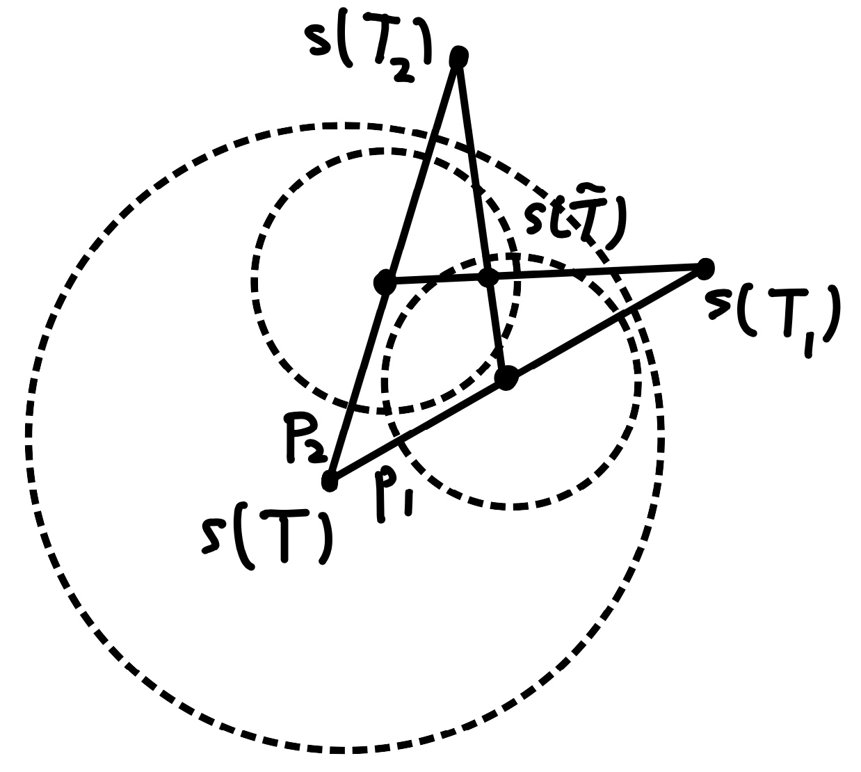
Figure 18. Example: adjuncts to verbs and semantic points.

With the construction of §2.2 and §3 of the extension $s:{\rm Dom}(h)\to{\mathcal{S}}$ of the map $s:{\mathcal{S}}{\mathcal{O}}_{0}\to{\mathcal{S}}$ we obtain points $s(T)\in{\mathcal{S}}$ and $s(T_{i})\in{\mathcal{S}}$ for each $i=1,\ldots,k$. When we consider each individual adjunct, the corresponding point

$$s_{i}:=s(\Tree[TT_{i}])$$

lies on the geodesic arc in ${\mathcal{S}}$ between $s(T)$ and $s(T_{i})$, at a distance $p_{i}={\mathbb{P}}_{\sigma}(s(T),s(T_{i}))$ from $s(T)$, where $\sigma$ is the adjunct syntactic relation. In particular, there is a convex geodesic neighborhood of the point $s(T)$ in ${\mathcal{S}}$ that contains all the points $s_{i}$. When we consider the combinations $T_{i_{1},\ldots,i_{r}}$ of the adjuncts $T_{i}$, this further determines points

$$s_{i_{1}\ldots i_{r}}=s(\Tree[T\quad T_{i_{1}\ldots i_{r}}])\,.$$

These points are contained in the same neighborhood of $s(T)$ and they are also contained in the intersection of neighborhoods around the points $s_{i}$ with $i\in\{i_{1},\ldots,i_{k}\}$. A sketch of this relation is illustrated in Figure 18, with

$$\tilde{T}:=\Tree[TT_{12}]\,.$$

Dropping the more refined metric/convexity structure, and the fact that the more precise location of this point depends on syntactic heads and evaluation of semantic proximity of the lexical items involved, if we only retain the Boolean relations of these neighborhoods and their intersections, we obtain a map to the Boolean semiring that checks the fact that “John ate a sandwich in the basement at noon” implies that “John ate a sandwich in the basement” and that “John ate a sandwich at noon”, while the opposite implications do not hold, as desired.

Here we can see, however, that the construction of the map $s:{\rm Dom}(h)\to{\mathcal{S}}$ that we used in §2.2 and §3 is only an oversimplified model, and that it should be refined by directly including coverings by neighborhoods related by intersections; see the discussion in §2.2.5.

6.2. Predicate saturation in Pietroski’s semantics and operadic structure

Other important parts of Pietroski’s semantics, in addition to the Combine operation discussed above, consists of predicate saturation and existential closure, see [73]. We propose here a way to fit these aspects in our model, compatibly with the form of the Combine operation that we just described, using the formulation of the magma ${\mathcal{S}}{\mathcal{O}}$ of syntactic objects in terms of operads (which we mentioned briefly in §1.2.2).

We recall briefly the mathematical notion of an operad, introduced in [68], and we describe how to view syntactic objects as an algebra over an operad.

6.2.1. Syntactic objects and operads

An operad (in Sets) is a collection ${\mathcal{O}}=\{{\mathcal{O}}(n)\}_{n\geq 1}$ of sets of $n$-ary operations (with $n$ inputs and one output), with composition laws

(6.3) $$\gamma:{\mathcal{O}}(n)\times{\mathcal{O}}(k_{1})\times\cdots\times{\mathcal{O}}(k_{n})\to{\mathcal{O}}(k_{1}+\cdots+k_{n})$$

that plug the output of an operation in ${\mathcal{O}}(k_{i})$ into the $i$-th input of an operation in ${\mathcal{O}}(n)$. The composition of these operations $\gamma$ is subjects to requirements of associativity and unitarity, which we do not write out explicitly here. An algebra ${\mathcal{A}}$ over an operad ${\mathcal{O}}$ (in Sets) is a set ${\mathcal{A}}$ on which the operations of ${\mathcal{O}}$ act, namely there are maps

(6.4) $$\gamma_{\mathcal{A}}:{\mathcal{O}}(n)\times{\mathcal{A}}^{n}\to{\mathcal{A}}$$

that satisfy compatibility with the operad composition,

(6.5) $$\begin{array}[]{c}\gamma_{\mathcal{A}}(\gamma_{\mathcal{O}}(T,T_{1},\ldots,T_{m}),a_{1,1},\ldots,a_{1,n_{1}},\ldots,a_{m,1},\ldots,a_{m,n_{m}})=\\[8.53581pt] \gamma_{\mathcal{A}}(T,\gamma_{\mathcal{A}}(T_{1},a_{1,1},\ldots,a_{1,n_{1}}),\ldots,\gamma_{\mathcal{A}}(T_{m},a_{m,1},\ldots,a_{m,n_{m}}))\,.\end{array}$$

for $T\in{\mathcal{O}}(m)$, $T_{i}\in{\mathcal{O}}(n_{i})$ and $\{a_{i,j}\}_{j=1}^{n_{i}}\subset{\mathcal{A}}$, and with $\gamma_{\mathcal{O}}$ the composition in the operad and $\gamma_{\mathcal{A}}$ the operad action. This notion means that elements of the set ${\mathcal{A}}$ can be used as inputs for the operations in ${\mathcal{O}}$, resulting in an output that is again an element in ${\mathcal{A}}$. The category of Sets can be replaced by more general symmetric monoidal categories. In particular we can consider cases where ${\mathcal{A}}$ is a topological space, or a vector space, which are suitable for the setting of semantic spaces. The description of the operadic composition laws that we mentioned in §1.2.2, in terms of the compositions $\circ_{i}:{\mathcal{O}}(n)\times{\mathcal{O}}(m)\to{\mathcal{O}}(n+m-1)$ is equivalent, for unitary operads, to the description in terms of the compositions (6.3).

In particular, we are interested here in the operad ${\mathcal{M}}$ freely generated by a single commutative binary operation ${\mathfrak{M}}$, where we have ${\mathcal{M}}(1)=\{{\rm id}\}$, ${\mathcal{M}}(2)=\{{\mathfrak{M}}\}$, ${\mathcal{M}}(3)=\{{\mathfrak{M}}\circ({\rm id}\times{\mathfrak{M}}),{\mathfrak{M}}\circ({\mathfrak{M}}\times{\rm id})\}$, etc. Consider again the set of syntactic objects ${\mathcal{S}}{\mathcal{O}}$. The magma structure of (1.1) can be reformulated as the structure of algebra over this operad.

Lemma 6.1.

The set ${\mathcal{S}}{\mathcal{O}}$ of syntactic objects is an algebra over the operad ${\mathcal{M}}$ freely generated by the single commutative binary operation ${\mathfrak{M}}$.

Proof.

We can identify the elements in ${\mathcal{M}}(n)$ with the abstract binary rooted trees with $n$ leaves (with no labels on the leaves), where each internal (non-leaf) vertex is labelled by an ${\mathfrak{M}}$ operation. The maps (6.8) are simply given by taking $\gamma(T,T_{1},\ldots,T_{n})$ with $T\in{\mathcal{M}}(n)$ and $T_{i}\in{\mathcal{S}}{\mathcal{O}}$ for $i=1,\ldots,n$ to be the abstract binary rooted tree in ${\mathfrak{T}}_{{\mathcal{S}}{\mathcal{O}}_{0}}={\mathcal{S}}{\mathcal{O}}$ obtained by grafting the root of the syntactic object $T_{i}$ to the $i$-th leaf of $T\in{\mathcal{M}}(n)$. If the syntactic objects $T_{i}$ have $n_{i}$ leaves, then the syntactic object $\gamma(T,T_{1},\ldots,T_{n})$ obtained in this way has $n_{1}+\cdots+n_{k}$ leaves. Note that this operad action is just a repeated application of the product operation ${\mathfrak{M}}$ in the magma ${\mathcal{S}}{\mathcal{O}}$, hence the description as algebra over ${\mathfrak{M}}$ and as magma as in (1.1) are equivalent. ∎

6.2.2. Semantic spaces and operads

The additional structure that we want to consider here, on the side of semantic spaces, is that of a partial algebra over the operad ${\mathcal{M}}$.

Definition 6.2.

Let ${\mathcal{M}}$ be the operad freely generated by a single commutative binary operation ${\mathfrak{M}}$. A semantic space ${\mathcal{S}}$ is a compositional semantic space if it has the following properties:

1. There is a map $s:{\rm Dom}(h)\to{\mathcal{S}}$ extending $s:{\mathcal{S}}{\mathcal{O}}_{0}\to{\mathcal{S}}$.

2. There is an action of the operad ${\mathcal{M}}$ on ${\mathcal{S}}$

   (6.6) $$\gamma_{\mathcal{S}}:{\mathcal{M}}(n)\times{\mathcal{S}}^{n}\to{\mathcal{S}}\,.$$

3. For $T\in{\mathcal{M}}(n)$ and for $T_{1},\ldots,T_{n}\in{\rm Dom}(h)\subset{\mathcal{S}}{\mathcal{O}}$ such that

   $$\gamma_{{\mathcal{S}}{\mathcal{O}}}(T,T_{1},\ldots,T_{n})\in{\rm Dom}(h)$$

   we have

   (6.7) $$\gamma_{\mathcal{S}}(T,s(T_{1}),\ldots,s(T_{n}))=s(\gamma_{{\mathcal{S}}{\mathcal{O}}}(T,T_{1},\ldots,T_{n}))\,.$$

The last condition ensures that the structure of ${\mathcal{S}}{\mathcal{O}}$ as an algebra over the operad ${\mathcal{M}}$ and the structure of ${\mathcal{S}}$ as a partial algebra over the same operad ${\mathcal{M}}$ are compatible through the map $s:{\rm Dom}(h)\to{\mathcal{S}}$ from syntax to semantics.

One can more generally consider partial actions of an operad and a corresponding notion of partial algebra over an operad (introduced in [52]), where the operad action (6.8) is defined on a subdomain ${\mathcal{A}}_{0}\subset{\mathcal{A}}$,

(6.8) $$\gamma_{\mathcal{A}}:{\mathcal{O}}(n)\times{\mathcal{A}}_{0}^{n}\to{\mathcal{A}}\,.$$

For a compositional semantic space as in Definition 6.2 the predicate saturation operation of Pietroski’s semantics, in a form compatible with syntactic Merge, can be can be interpreted as the operad action (6.6) that saturates the arguments of an $n$-ary operation by inputs in ${\mathcal{S}}_{0}$ (a concept of adicity $n$ combined with $n$ semantic arguments). The partial compositions $\circ_{i}$ correspondingly give the combinations of a concept of adicity $n$ with one semantic argument that give a concept of adicity $n-1$. Note, however, that there is an important difference here. In this model the operations of adicity $n$ in ${\mathcal{M}}(n)$ are part of the syntax core computational mechanism. They are not on the semantic side, so they cannot directly be identified with the “concept of adicity $n$” described in [73]. It is only through the relation (6.7) that they acquire that role.

6.2.3. Syntax-driven compositional semantics

The notion of compositional semantic space that we described in Definition 6.2 is based on two operad actions, one (that we called $\gamma_{\mathcal{S}}{\mathcal{O}}$) on the side of syntax and one (that we called $\gamma_{\mathcal{S}}$) on the side of semantics, with the compatibility (6.7). This is similar to the formulation of Pietroski’s semantics in [73]. However, we show now that in fact the operad action $\gamma_{{\mathcal{S}}{\mathcal{O}}}$ on syntax suffices to completely determine its counterpart $\gamma_{\mathcal{S}}$.

Proposition 6.1.

Let ${\mathcal{S}}^{+}={\mathcal{S}}\cup\{s_{\infty}\}$ be the Alexandrov one-point compactification of ${\mathcal{S}}$, where we denote the added point with the symbol $s_{\infty}$. The action of the operad ${\mathcal{M}}$ on syntactic objects, described in Lemma 6.1, together with a function $s:{\rm Dom}(h)\to{\mathcal{S}}$ uniquely determine an action of the operad ${\mathcal{M}}$ on ${\mathcal{S}}$ by setting

(6.9) $$\gamma_{\mathcal{S}}(T,s_{1},\ldots,s_{n}):=\left\{\begin{array}[]{ll}s(\gamma_{{\mathcal{S}}{\mathcal{O}}}(T,T_{1},\ldots,T_{n}))&\text{if }\,s_{i}=s(T_{i})\text{ and }\gamma_{{\mathcal{S}}{\mathcal{O}}}(T,T_{1},\ldots,T_{n})\in{\rm Dom}(h)\\[8.53581pt] s_{\infty}&\text{otherwise.}\end{array}\right.$$

for $T\in{\mathcal{M}}(n)$ and $s_{1},\ldots,s_{m}\in{\mathcal{S}}^{+}$.

Proof.

We construct $\gamma_{\mathcal{S}}$ using $\gamma_{{\mathcal{S}}{\mathcal{O}}}$ and the compatibility relation (6.7) using (6.9), In order to show that (6.9) does indeed define an operad action on ${\mathcal{S}}$, we need to check the compatibility of $\gamma_{\mathcal{S}}$ with the operad composition $\gamma$ in ${\mathcal{M}}$, given by the condition (6.5). The left-hand-side of (6.5) gives

(6.10) $$\gamma_{\mathcal{S}}(\gamma_{{\mathcal{M}}}(T,T_{1},\ldots,T_{m}),s_{1,1},\ldots,s_{1,n_{1}},\ldots,s_{m,1},\ldots,s_{m,n_{m}})\,.$$

This is equal to $s_{\infty}$ unless both of the two conditions

• all the $s_{i,j}=s(T_{i,j})$ for some $T_{i,j}$ in ${\rm Dom}(h)\subset{\mathcal{S}}{\mathcal{O}}$;

• the syntactic object

  (6.11) $$\gamma_{{\mathcal{S}}{\mathcal{O}}}(\gamma_{{\mathcal{M}}}(T,T_{1},\ldots,T_{m}),T_{1,1},\ldots,T_{1,n_{1}},\ldots,T_{m,1},\ldots,T_{m,n_{m}})$$

  is in ${\rm Dom}(h)$

are satisfied, in which case (6.10) is equal to

(6.12) $$s(\gamma_{{\mathcal{S}}{\mathcal{O}}}(\gamma_{{\mathcal{M}}}(T,T_{1},\ldots,T_{m}),T_{1,1},\ldots,T_{1,n_{1}},\ldots,T_{m,1},\ldots,T_{m,n_{m}}))\,.$$

The compatibility of the action $\gamma_{{\mathcal{S}}{\mathcal{O}}}$ with the operad composition implies that (6.11) is equal to

(6.13) $$\gamma_{{\mathcal{S}}{\mathcal{O}}}(T,\gamma_{{\mathcal{S}}{\mathcal{O}}}(T_{1},T_{1,1},\ldots,T_{1,n_{1}}),\ldots,\gamma_{{\mathcal{S}}{\mathcal{O}}}(T_{m},T_{m,1},\ldots,T_{m,n_{m}}))\,.$$

Note that if the full composition in (6.11) is in ${\rm Dom}(h)$ by the properties of abstract head functions all the substructures $\gamma_{{\mathcal{M}}}(T_{i},T_{i,1},\ldots,T_{i,n_{i}})$, $i=1,\ldots,m$, are also in ${\rm Dom}(h)$. Thus, the point (6.12) in ${\mathcal{S}}$ is the same as the point

$$s(\gamma_{{\mathcal{S}}{\mathcal{O}}}(T,\gamma_{{\mathcal{S}}{\mathcal{O}}}(T_{1},T_{1,1},\ldots,T_{1,n_{1}}),\ldots,\gamma_{{\mathcal{S}}{\mathcal{O}}}(T_{m},T_{m,1},\ldots,T_{m,n_{m}})))=$$

$$\gamma_{\mathcal{S}}(T,s(\gamma_{{\mathcal{S}}{\mathcal{O}}}(T_{1},T_{1,1},\ldots,T_{1,n_{1}})),\ldots,s(\gamma_{{\mathcal{S}}{\mathcal{O}}}(T_{m},T_{m,1},\ldots,T_{m,n_{m}})))=$$

$$\gamma_{\mathcal{S}}(T,\gamma_{\mathcal{S}}(T_{1},s_{1,1},\ldots,s_{1,n_{1}}),\ldots,\gamma_{\mathcal{S}}(T_{m},s_{m,1},\ldots,s_{m,n_{m}}))\,,$$

which gives the right-hand-side of (6.5). ∎

The structure of algebra over the operad ${\mathcal{M}}$ on ${\mathcal{S}}^{+}$ makes ${\mathcal{S}}$ a partial algebra over ${\mathcal{M}}$.

Note that we are everywhere somewhat simplifying the picture, as we do not include the possibility that different syntactic objects in ${\rm Dom}(h)\subset{\mathcal{S}}{\mathcal{O}}$ may sometime map to the same value in ${\mathcal{S}}$ under $s:{\rm Dom}(h)\to{\mathcal{S}}$ and also the possibilities of ambiguities of semantic assignment where $s:{\rm Dom}(h)\to{\mathcal{S}}$ may sometimes be multivalued. These possibilities would affect the construction (6.9) of $\gamma_{\mathcal{S}}$ and would require a modified argument.

6.3. Adjunction, embedded constructions, and the Pair-Merge problem

Our model of the map $s:{\rm Dom}(h)\to{\mathcal{S}}$, that extends the assignment $s:{\mathcal{S}}{\mathcal{O}}_{0}\to{\mathcal{S}}$ of semantic values defined on lexical items, is a very simple model built using only the head function and proximity relations (and geodesic distance) in semantic space ${\mathcal{S}}$. In particular, since we start with the syntactic objects produced by the free symmetric Merge, the only factor that introduces asymmetry in this construction is coming from the head function.

We discuss here briefly how one can try, within the limits of such an oversimplified model, to address the question of misalignments between hierarchical syntax and compositional semantics that occur as a consequence of the particular behavior of adjunction, and in particular what is sometimes referred to as the invisibility of adjuncts to syntax. This question was posed to us by Riny Huijbregts.

A proposal for handling this type of problem is to postulate the existence of an asymmetrical Pair-Merge operation accounting for argument-adjunct asymmetry (see [10]), in addition to the free symmetric Merge. This proposal has undesirable features, as it requires the introduction of an additional form of asymmetric Merge dealing with the peculiar behavior of adjunction, while one expects that the computational mechanism of syntax should just rely entirely on the free symmetric Merge. An alternative proposal (see for instance [71]) involves the use of “two-peaked” structures (see Figure 19) with $\{XP,YP\}$ an adjunction. This proposal has the drawback that, if one considers such “two-peaked” structures as part of syntax, then one needs to justify them in terms of the free Merge generative process, and this is problematic because the elements of the magma ${\mathcal{S}}{\mathcal{O}}={\mathfrak{T}}_{{\mathcal{S}}{\mathcal{O}}_{0}}$ do not contain such structures, nor does the action of Merge on workspaces (as can be also seen in the formalization given in our paper [61]). The proposal of “two-peaked” structures in [71] is based on [29], but is not formulable within the generative process of a free symmetric Merge. We are going to discuss briefly what this means in terms of our model.

The reason why adjunction appears problematic in our setting is that adjunction can be seen as an instance of syntactic objects $\{XP,YP\}$ which do not have a well defined head function in the sense we have been using above, $\{XP,YP\}\notin{\rm Dom}(h)$. This creates a problem with our simple model of mapping to semantics, which is defined only on ${\rm Dom}(h)$. We want to argue here that this problem can be to some extent bypassed without the need to significantly alter the construction of the mapping $s:{\rm Dom}(h)\to{\mathcal{S}}$, although, of course we expect that the naive model for this map based on the datum of the head function may be replaced by some more elaborate versions.

Suppose given a syntactic object of the form $\{XP,YP\}\notin{\rm Dom}(h)$, where both $XP$ and $YP$ are in ${\rm Dom}(h)$. In terms of our construction, the fact that the head function is not well defined on the object $\{XP,YP\}$ implies that we do not have a choice of orientation on the geodesic arc between $s(XP)$ and $s(YP)$ in ${\mathcal{S}}$ and a corresponding point along this arc at a distance ${\mathbb{P}}(s(XP),s(YP))$ from the image of the head. We do still have the geodesic arc, though, and the measurement ${\mathbb{P}}(s(XP),s(YP))$ of syntactic relatedness between its endpoints. So in terms of this construction, all that a hypothetical asymmetric Pair-Merge would provide is a choice of orientation on the geodesic arc. Such a datum is a geometric datum in ${\mathcal{S}}$ and does not necessarily require the existence of Pair-Merge as an additional part of the computational structure of syntax. One can extend $s:{\rm Dom}(h)\to{\mathcal{S}}$ to a slightly larger domain that includes adjunctions just by the requirements that geodesic arcs in ${\mathcal{S}}$ whose endpoints are the two terms of an adjunction come with a preferred choice of orientation. This choice has the same effect of a Pair-Merge $\langle XP,YP\rangle$ signifying that the first element should be taken to be the “head” while the second element is to be seen as an “adjunct”. Such choice of orientation then ensures that we can extend the same construction of $s:{\rm Dom}(h)\to{\mathcal{S}}$ also to adjunctions $\{XP,YP\}\notin{\rm Dom}(h)$. In general one does not expect that this orientation requirement should be extendable to other types of syntactic objects $\{XP,YP\}\notin{\rm Dom}(h)$ that are not adjunctions. The fact that this mechanism does not require any modification of the syntactic generative process and only involves a metric property in ${\mathcal{S}}$ is consistent with the idea that adjuncts are on a “separate plane” (see [10]).

While this approach can be accommodated within our setting, it leaves open the question of assigning general criteria for orientations of geodesic arcs in ${\mathcal{S}}$ that generalize the choice resulting from a had function, incorporating the case of adjunctions, but not the case of arbitrary $\{XP,YP\}$ objects.

Thinking in terms of “two-peaked” structures, on the other hand, presents another possibility for treating this problem of adjunctions in our geometric setting. Given a syntactic object of the form $\{XP,YP\}\notin{\rm Dom}(h)$, where both $XP$ and $YP$ are in ${\rm Dom}(h)$, consider in ${\mathcal{S}}$ the points $s(XP)$ and $s(YP)$ and the geodesic arc between them (now without any preferred assignment of orientation). Suppose given also a syntactic object $T=\{Z,XP\}\in{\rm Dom}(h)$. Since this is in the domain of the head function, it defines a point $s(T)$ on the geodesic arc between $s(Z)$ and $s(XP)$, where the geodesic arc is oriented from the end that corresponds to the head to the other. Thus, we do indeed obtain a “two-peaked” structure, as in Figure 19. Note that, while the geodesic arc between $s(XP)$ and $s(YP)$ does not have an a priori choice of orientation, the orientation induced by the head on the geodesic arc between $s(Z)$ and $s(XP)$ induces a unique consistent orientation on the arc between $s(XP)$ and $s(YP)$.

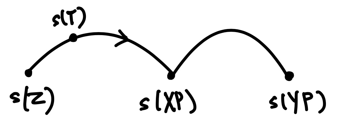
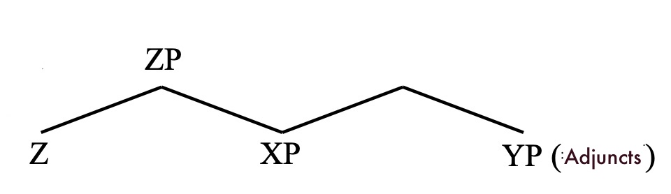
Figure 19. “Two-peaked” structures inside ${\mathcal{S}}$.

It is important to stress here the difference between the type of “two-peaked” structures we are describing and the proposed “two-peaked” structures in the syntactic setting, as in [71]. Here this structure does not exist in the magma ${\mathcal{S}}{\mathcal{O}}$, it only exists in the image of syntax under the map to semantic space ${\mathcal{S}}$. In other word, these “two-peaked” structures are not part of the computational process of syntax and do not need to be justified by any additional form of Merge. They exist because the images of syntactic objects inside ${\mathcal{S}}$ can intersect, even though the resulting configuration (like the one in Figure 19) is not itself the image of a syntactic object.

7. No, they don’t: transformers as characters

Recently, it has become fashionable to claim that the so-called transformer architectures underlying the functioning of many current large language models (LLMs) somehow “disprove” or undermine the theory of generative linguistics. They don’t. Such claims are vacuous: not only on account that they lack any accurate description of what is allegedly being disproved, but also more specifically because one can show, as we will discuss in this section, that the functioning of the attention modules of transformer architectures fits remarkably well within the same general formalism we have been illustrating in the previous sections, and is consequently fully compatible with a generative model of syntax based on Merge and Minimalism. While this can be discussed more at length elsewhere, we will show here briefly that the weights of attention modules in transformer architectures can be regarded as another (distinct from human) way of embedding an image of syntax inside semantics, with formal properties similar to other examples we talked about earlier in this paper.

This does not mean, of course, that LLMs based on such architectures necessarily mimic the interaction between syntax and semantics as it occurs in human brains. In fact, most certainly that is not the case in anything close to their present form, given well known considerations regarding the “poverty of the stimulus,” in human language acquisition (see [4]), compared to what one may call the “overwhelming richness of the stimulus” in the training of LLMs. Some have attempted to deal with this issue by limiting the amount of training data to something argued to align more with the data available to children (e.g., as in [83] and [47], among others, including an upcoming 2023CoNLL/CMCL “Baby LMChallenge” [2]). However, at least so far there are still problems with such approaches with regard to both performance on certain test-bed datasets, and accurately mirroring the developmental trajectory of human language acquisition, with respect to training data sample sizes. This matter is discussed in more detail in [85].

This is not the main point of the discussion here, however, since several examples we analyzed in the previous sections are also not meant to model how syntax and semantics realistically interact in the human brain, but are presented simply as illustrations of the general formal algebraic properties of the mathematical model. The point we intend to make here is that attention modules of transformer architectures can function as another choice of a Hopf algebra character that fits within the same very general algebraic formalism we illustrated in the previous sections of this paper. Therefore, transformer architectures have no intrinsic incompatibility, at this fundamental algebraic level, with generative syntax. Note also that we are not going to include here any discussion with regard to the efficiency of computational algorithms, as we are interested only in analyzing their algebraic structure. We will only make some general comments at the end of this section, in relation to the “inverse problem” of reconstructing syntax from its image inside semantics, that we already discussed in §3.

For our purposes, it suffices to consider the basic fundamental functioning of attention modules in transformers, that we recall schematically as follows.

We assume, as in our previous setting in §2, a given function $s:{\mathcal{S}}{\mathcal{O}}_{0}\to{\mathcal{S}}$ from lexical items and syntactic features to a semantic space ${\mathcal{S}}$ that is here assumed to be a vector space model. Thus, we can view elements $\ell\in{\mathcal{S}}{\mathcal{O}}_{0}$ as vectors $s(\ell)\in{\mathcal{S}}$. In attention modules, in the case of so-called self-attention that we focus on here, one considers three linear transformations: $Q$ (queries), $K$ (keys), and $V$ (values), $Q,K\in\operatorname*{Hom}({\mathcal{S}},{\mathcal{S}}^{\prime})$ and $V\in\operatorname*{Hom}({\mathcal{S}},{\mathcal{S}}^{\prime\prime})$, where ${\mathcal{S}}^{\prime}$ and ${\mathcal{S}}^{\prime\prime}$ are themselves vector spaces of semantic vectors (in general of dimensions not necessarily equal to that of ${\mathcal{S}}$).

One usually assumes given identifications ${\mathcal{S}}\simeq{\mathbb{R}}^{n}$, ${\mathcal{S}}^{\prime}\simeq{\mathbb{R}}^{m}$, ${\mathcal{S}}^{\prime\prime}\simeq{\mathbb{R}}^{d}$ with Euclidean vector spaces, with assigned bases, and one works with the corresponding matrix representations of $Q,K\in\operatorname*{Hom}({\mathbb{R}}^{n},{\mathbb{R}}^{m})$ and $V\in\operatorname*{Hom}({\mathbb{R}}^{n},{\mathbb{R}}^{d})$. The target Euclidean space ${\mathcal{S}}^{\prime}$ is endowed with an inner product $\langle\cdot,\cdot\rangle$, that can be used to estimate semantic similarity.

The query vector $Q(s(\ell))$, for $\ell\in{\mathcal{S}}{\mathcal{O}}_{0}$, can be thought of performing a role analogous to the semantic probes discussed in our toy models of §2. As in that case, we think of queries (or probes in our previous terminology) as elements $q\in{\mathcal{S}}^{\vee}$ where ${\mathcal{S}}^{\vee}$ is the dual vector space ${\mathcal{S}}^{\vee}=\operatorname*{Hom}({\mathcal{S}},{\mathbb{R}})$, so that a query matrix can be identified with an element in ${\mathcal{S}}^{\vee}\otimes{\mathbb{R}}^{m}\simeq{\mathcal{S}}^{\vee}\otimes{\mathcal{S}}^{\prime}=\operatorname*{Hom}({\mathcal{S}},{\mathcal{S}}^{\prime})$, that we can regard as an $m$-fold probe $Q$ evaluated on the given semantic vector $s(\ell)$.

In a similar way, we can think of the key vector $K(s(\ell))$, for $\ell\in{\mathcal{S}}{\mathcal{O}}_{0}$, also as an element $K\in\operatorname*{Hom}({\mathcal{S}},{\mathcal{S}}^{\prime})$, that we interpret in this case as a way of creating an $m$-fold probe out of the given vector $s(\ell)$. Thus, the space ${\mathcal{S}}^{\prime}$ of ($m$-fold) probes plays a dual role here, as given probes to be evaluated on an input semantic vector $s(\ell)$, and as new probes generated by the semantic vector $s(\ell)$. This dual interpretation explains the use of the terminology “query” and “key” for the two given linear transformations. The values vector $V(s(\ell))$ can be viewed as a representation of the semantic vectors $s(\ell)$ inside ${\mathcal{S}}^{\prime\prime}$, such as, for example, an embedding of the set $s(L)$, for a given subset $L\subset{\mathcal{S}}{\mathcal{O}}_{0}$, into a vector space ${\mathcal{S}}^{\prime\prime}$, of dimension lower than ${\mathcal{S}}$. One refers to $d=\dim{\mathcal{S}}^{\prime\prime}$ as the embedding dimension.

Next, one considers a set $L\subset{\mathcal{S}}{\mathcal{O}}_{0}$. Usually, this is regarded as an ordered set, a list (also called a string), that would correspond to an input sentence. However, in our setting, it is more convenient to consider $L$ as an unordered set. In terms of transformer models, one then focuses on bi-directional architectures like BERT. To an element $\ell\in L$ one assigns an attention operator $A_{\ell}:L\subset{\mathcal{S}}\to{\mathcal{S}}^{\prime}$, given by

$$A_{\ell}(s(\ell^{\prime}))=\sigma(\langle Q(s(\ell)),K(s(\ell^{\prime}))\rangle)\,,$$

where $\sigma$ is the softmax function $\sigma(x)_{i}=\exp(x_{i})/\sum_{j}\exp(x_{j})$, for $x=(x_{i})$.

Note that for simplicity of notation, we are ignoring here the usual rescaling factor that divides by the square root of the embedding dimension, since that has no influence on the algebraic structure of the model, even through it has computational significance. We write $A_{\ell,\ell^{\prime}}:=A_{\ell}(s(\ell^{\prime}))$ and refer to it as the attention matrix. The matrix entries $A_{\ell,\ell^{\prime}}$ are regarded as a probability measure of how the attention from position $\ell$ is distributed towards the other positions $\ell^{\prime}$ in the set $L$. One then assigns an output (in ${\mathcal{S}}^{\prime\prime}$) to the input $s(L)\subset{\mathcal{S}}$, as the vectors $y_{\ell}=\sum_{\ell^{\prime}}A_{\ell,\ell^{\prime}}V(s(\ell^{\prime}))$, where for each $\ell\in L$, we have $y_{\ell}=(y_{\ell})_{i=1}^{d}\in{\mathcal{S}}^{\prime\prime}\simeq{\mathbb{R}}^{d}$.

Observe that in writing $A$ as a matrix one uses a choice of ordering of the set $L$, but the linear operator $A_{\ell}$ itself is defined independently of such an ordering. Compatibly with the fact that we want to use free symmetric Merge as generator of syntactic objects, we indeed focus here on the case of bidirectional, non-causal attention, where the non-trivial entries of the attention matrix are not limited to items occurring in a specified linear order (i.e. the matrix is not necessarily lower or upper diagonal in a chosen basis/ordering). The resulting $y_{\ell}$ is symmetric in the ordering of $L$, so linear ordering also does not play a role in the output.

7.0.1. Heads and heads

In transformer architectures, one usually has several such attention modules running in parallel, and one refers to this setting as multi-head attention. In this case, the vectors $Q(s(\ell))=\oplus_{i}Q(s(\ell))_{i}$, $K(s(\ell))=\oplus_{i}K(s(\ell))_{i}$, and $V(s(\ell))=\oplus_{j}V(s(\ell))_{j}$ are split into blocks, that correspond to a decomposition ${\mathcal{S}}^{\prime}=\oplus_{i=1}^{N}{\mathcal{S}}^{\prime}_{i}$, and similarly for ${\mathcal{S}}^{\prime\prime}$, with the inner product of ${\mathcal{S}}^{\prime}$ compatible with the direct sum decomposition, inducing inner products $\langle\cdot,\cdot\rangle_{{\mathcal{S}}^{\prime}_{i}}$. One can then compute attention matrices, for $i=1,\ldots,N$,

$$A^{(i)}_{\ell,\ell^{\prime}}=\sigma(\langle Q(s(\ell))_{i},K(s(\ell))_{i}\rangle_{{\mathcal{S}}^{\prime}_{i}})$$

that one refers to as attention distribution with attention head $i$.

It is important to keep in mind that there is an unfortunate clash of notation here, between this meaning of “head” as “attention head” versus the usual syntactic meaning of “syntactic head”, represented in the present paper by the notion of “head function” in Definition 1.1.

For simplicity, and to avoid confusing notation, we will not consider here multiple attention heads, and work only with a single attention matrix, that suffices for our illustrative purposes, while we will be referring to the term head only in its syntactic meaning as a head function.

7.1. Maximizing attention

Since for fixed $\ell\in L$ the values $A_{\ell,\ell^{\prime}}$ give a probability measure on $L$, we can consider characters with values in the semiring ${\mathcal{R}}=([0,1],\max,\cdot)$. For example, it is natural to look for where the attention from position $\ell$ is maximized. Thus, we can define a character on a subdomain

$$\phi_{A}:{\mathcal{H}}^{semi}\to{\mathcal{R}}$$

by setting

$$\phi_{A}(T)=\max_{\ell\in L(T)}A_{h(T),\ell}\,,$$

if $T\in{\rm Dom}(h)$ and zero otherwise.

Remark 7.1.

Note that, in order to make $\phi$ well defined for all $T\in{\mathfrak{T}}_{{\mathcal{S}}{\mathcal{O}}_{0}}$, we need a uniform choice of the operator $A_{\ell}$ for an $\ell\in L(T)$, that is to say, we need a consistent way of extracting the choice of a leaf from each tree. This corresponds to the choice of a head function $h$ in the sense of Definition 1.1.

Once a head function $h$ is chosen, the attention matrix determines an associated attention vector $A_{h(T),\ell}$ for $\ell\in L(T)$. In particular, we can choose the head function to be the same as the syntactic head, although this is not necessary and any choice of a head function will work for this purpose. Note that head functions are not everywhere defined on ${\mathfrak{T}}_{{\mathcal{S}}{\mathcal{O}}_{0}}$. This implies that the choice of attention vector cannot be made compatibly with substructures simultaneously across all trees $T\in{\mathfrak{T}}_{{\mathcal{S}}{\mathcal{O}}_{0}}$. There is some maximal domain ${\rm Dom}(h)\subset{\mathfrak{T}}_{{\mathcal{S}}{\mathcal{O}}_{0}}$ over which such a consistent choice can be made. This issue does not arise in the construction of attention matrices from text, as sentences in text will always have a syntactic head, but it can be relevant when sentences are stochastically generated from a template (such as those used in tests of linguistic capacities of LLMs, as in [83], [47]).

7.2. Attention-detectable syntactic relations

Recent investigation of attention modules and syntactic relations (like c-command, see [58]) indicate that syntactic trees and examples of specific syntactic relations such as syntactic head, prepositional object, possessive noun, and the like, are embedded and detectable from the attention matrix data. We show that this result is to be expected, given our model.

We consider the problem of detection of syntactic relations in the following form.

Definition 7.2.

Suppose given a syntactic relation $\rho$, which we write as a collection $\rho=\rho_{T}$ of relations $\rho_{T}\subset L(T)\times L(T)$, with $\rho_{T}(\ell,\ell^{\prime})=1$ is $\ell,\ell^{\prime}\in L(T)$ are in the chosen relation and $\rho_{T}(\ell,\ell^{\prime})=0$ otherwise. We say that $\rho$ is exactly attention-detectable if there exist query/key linear maps $Q_{\rho},K_{\rho}\in\operatorname*{Hom}({\mathcal{S}},{\mathcal{S}}^{\prime})$ and there exists a head function $h_{\rho}$ as in Definition 1.1 such that

$$\rho_{T}(h_{\rho}(T),\ell_{\max,h_{\rho}})=1$$

for all $T\in{\rm Dom}(h_{\rho})$, where

$$\ell_{\max,h_{\rho}}={\rm argmax}_{\ell\in L(T)}A_{h_{\rho}(T),\ell}\,,$$

with $A$ the attention matrix built from $Q_{\rho},K_{\rho}$.

The relation $\rho$ is approximately attention-detectable if there exist query/key linear maps $Q_{\rho},K_{\rho}\in\operatorname*{Hom}({\mathcal{S}},{\mathcal{S}}^{\prime})$ and there exists a head function $h_{\rho}$ as in Definition 1.1 such that

$$\frac{1}{\#{\mathcal{D}}}\sum_{T\in{\mathcal{D}}}\rho(h_{\rho}(T),\ell_{\max,h_{\rho}})\sim 1$$

for some sufficiently large set ${\mathcal{D}}\subset{\rm Dom}(h_{\rho})$ of trees.

Here the existence of query/key linear maps $Q_{\rho},K_{\rho}$ as above is relative to a specified context, such as a corpus, a dataset.

In the case of approximately attention-detectable syntactic relations, we think of the subset ${\mathcal{D}}$ as being, for instance, a sufficiently large syntactic treebank corpus, or a corpus of annotated syntactic dependencies (for size estimates see [58]). Cases where the existence of query/key linear maps $Q_{\rho},K_{\rho}$ and a head function $h_{\rho}$ with the properties required above can be ensured can be extracted from the experiments in [58].

7.3. Threshold Rota-Baxter structures and attention

Using a threshold Rota-Baxter operator $c_{\lambda}$ of weight $+1$, we obtain

$$\phi_{A,-}(T)=c_{\lambda}(\max\{\phi_{A}(T),c_{\lambda}(\phi_{A}(F_{\underline{v}}))\cdot\phi_{A}(T/F_{\underline{v}}),\ldots,c_{\lambda}(\phi_{A}(F_{\underline{v_{N}}}))\cdot\phi_{A}(F_{\underline{v}_{N-1}}/F_{\underline{v_{N}}})\cdots\phi_{A}(T/F_{\underline{v}_{1}})\})\,.$$

As above, for simplicity we focus on the case of chains of subtrees $T_{v_{N}}\subset T_{v_{N-1}}\subset\cdots\subset T_{v_{1}}\subset T$ rather than more general subforests. Note that $h(T/T_{v})=h(T)$ for the quotient given by contraction of the subtree, hence

$$\max_{\ell\in L(T/T_{v})}A_{h(T),\ell}\leq\max_{\ell\in L(T)}A_{h(T),\ell}\,.$$

The value $\phi_{-}(T)$ corresponds then to the chains of nested accessible terms of the syntactic object $T$ for which all the values

$$\phi_{A}(T_{v_{i}})=\max_{\ell\in L(T_{v_{i}})}A_{h(T_{v_{i}}),\ell}$$

are above the chosen threshold $\lambda$ and all the complementary quotients $T_{v_{i-1}}/T_{v_{i}}$ have

$$\phi_{A}(T_{v_{i-1}}/T_{v_{i}})=\max_{\ell\in L(T_{v_{i-1}}/T_{v_{i}})}A_{h(T_{v_{i-1}),\ell}}=\max_{\ell\in L(T_{v_{i-1}})}A_{h(T_{v_{i-1}}),\ell}=\phi_{A}(T_{v_{i-1}})\,.$$

The first condition implies that one is selecting only chains of accessible terms inside the syntactic object $T$ where the maximal attention from the head of each subtree in the chain is sufficiently large, while the second condition means that, among these chains one is selecting only those for which the recipient of maximal attention from the head of the given subtree is located outside of the next subtree. This second condition guarantees that when considering the next nested subtree and trying to maximize for its attention value, one does not spoil the optimizations achieved at the previous steps for the larger subtrees.

A similar procedure can be obtained by additionally introducing direct implementation of some syntactic constraints. We can see this in the following way.

A syntactic relation $\rho$ determines a character $\phi_{\rho}$ on trees $T\in{\rm Dom}(h)\subset{\mathfrak{T}}_{{\mathcal{S}}{\mathcal{O}}_{0}}$ with values in the Boolean ring ${\mathcal{B}}=(\{0,1\},\max,\cdot)$ where

$$\phi_{\rho}(T)=\max_{\ell\in L(T)}\rho(h(T),\ell)\,.$$

This Boolean character detects whether the syntactic relation $\rho$ is realized in the tree $T$ or not.

Using a character

$$\phi_{A,\rho}(T)=\max_{\ell\in L(T)}\rho(h(T),\ell)\cdot A_{h(T),\ell}\,,$$

with values in ${\mathcal{P}}=([0,1],\max,\cdot)$, one maximizes the attention from the tree head over the set of $\ell\in L(T)$ that already satisfy the chosen syntactic relation with respect to the head of the tree. The corresponding Birkhoff factorization with threshold Rota-Baxter operators again identifies chains of subtrees that maximize the attention (above a fixed threshold), in a way that is recursively compatible with the larger trees as before, but where now maximization is done only on the set where the relation is implemented. Subtrees with $\phi_{\rho}(T_{v})=0$ do not contribute even if their value of $\max_{\ell}A_{h(T),\ell}$ is sufficiently large.

Thus, comparison between the case with character $\phi_{A}$ and with character $\phi_{A,\rho}$ identify attention-detectability of the syntactic property considered and, if detectability fails, at which level in the tree (in terms of chains of nested subtrees) the attention matrix maximum happens outside of where the syntactic relation holds.

As shown in [85], the current performance on syntactic capacities of LLMs trained on small scale data modeling falls significantly short of the human performance, when tested on LI-Adger datasets that include sufficiently diverse syntactic phenomena. This suggests a good testing ground for syntactic recoverability as outlined above and a possible experimental testing for aspects of the inverse problem of the syntax-semantics interface.

7.3.1. Syntax as an inverse problem: physics as metaphor

The question of reconstructing the computational process of syntax, in LLMs based on transformer architectures, can be seen in the same light as the situation we illustrated in a simpler example in §3, where one views the image of syntax embedded inside a semantic space, and considers the inverse problem of extracting syntax as a computational process working from these images, which live in a semantic space that is not itself endowed with the same type of computational structure. Here, the image of syntax is encoded in the key/query vectors that live in vector spaces that organize semantic proximity data, and in the resulting attention matrices. Inverse problems of this kind are usually expected to be computationally hard. This does not mean that the computational mechanism of syntax cannot be reconstructible, but that a significant cost in complexity, growing rapidly with the depth of the trees, may be involved.

Early results showed that RNN language models performed poorly on tests of grammaticality aimed at capturing syntactic structures, on a testbed dataset of pairs of sentences that differ only in their grammaticality, [67], while [42] showed that language models based on RNNs can perform well on predicting long-distance number agreement even in the absence of semantic clues (that is, when tested on nonsensical but grammatical sentences). Results like this appear to indicate that syntax can, in principle, be extracted and disentangled from its image inside semantics. It was shown in [79] that Syntactic Ordered Memory (SOM) syntax-aware language models outperform the Chat-GPT2 LLM in syntactic generalization tests. However, this entire area remains a matter of contention, dependent in part on the testbed dataset used, as described more fully in [84] and [85].

A more systematic comparison of different language model architectures and their performance on syntactic tests in [46] revealed substantial differences in syntactic generalization performance by model architecture, more than by size of the dataset. One can suggest that the indicators of poor performance on syntactic tests, along with any other difficulties, might also reflect the computational difficulty involved in extracting syntax as an inverse problem from its image through the semantic interface, stored across values of the weights of attention matrices, rather than in a direct syntax-first mapping.

In this paper we have used physics as a guideline for identifying mathematical structures that can be useful in modelling the relation between syntax and semantics. We conclude here by using physics again, this time only as a metaphor, for describing the relation of syntax as a generative process and the functioning of LLMs.

The generative structure underlying particle physics is given by the Feynman diagrams of quantum field theory. Disregarding epistemological issues surrounding the interpretation of such diagrams as events of particle creation and decay, we can roughly say that, in a particle physics experiment, what one detects is an image of such objects embedded into the set of data collected by detectors. Detecting a particle, say the Higgs boson (the most famous recent particle physics discovery), means solving an inverse problem that identifies inside this enormous set of data the traces of the correct diagrams/processes involving the creation of a Higgs particle from an interaction of other particles (such as gluon fusion or vector-boson fusion) and its subsequent decay into other particles (such as vector-boson pairs or photons). The enormous computational difficulty implicit in this task arises from the need to solve this type of inverse problem, involving the identification of events structure (for example a Higgs decay into photons involving top quark loop diagrams) from the measurable data, and a search for the desired structure in a background involving a huge number of other simultaneous events. The direct map from quantum field theory consists of the Higgs boson production cross sections, which are calculated from perturbative expansions in the Feynman diagrams of quantum chromodynamics and quantum electrodynamics, involving significant higher-order quantum corrections. Such perturbative QFT computations are where the algebraic formalism recalled at the beginning of this paper plays a role. The inverse problem, instead, consists of measuring, for various possible decay channels, mass and kinematic information like decay angles of detectable particles of the expected type, produced either by the expected decay event or by the background of productions of the same particle types due to other events, and searching for an actual signal in this background.

We can use this story as a metaphor, and imagine the generative process of syntax embedded inside LLMs in a conceptually similar way, its image scattered across a probabilistic smear over a large number of weights and vectors, trained over large data sets. This view of LLMs as the technological “particle accelerators” of linguistics, where signals of linguistic structures are detectable against a background of probabilistic noise, suggests that such models do not invalidate generative syntax any more than particle detectors would “invalidate” quantum field theory; quite the contrary in fact.

While LLMs do not constitute a model of language in the human brain, they can still, in the sense described here, provide an apparatus for the experimental study of inverse problems in the syntax-semantic interface. Here however it is essential to recall again the physics metaphor. Data and technology without theory do not constitute science, understood as a model of the fundamental laws of nature that has both strong predictive capacity and a high level of concise conceptual clarity in its explanatory power. The relation between the computational process of syntax and the topological relational nature of semantics is a problem of a conceptual nature. In this sense, the large language models may contribute a technological experimental laboratory for the analysis of some aspects of this problem, rather than a replacement for the necessary theoretical understanding of fundamental laws in the structure of language.

Acknowledgments

The first author acknowledges support from NSF grant DMS-2104330 and FQXi grants FQXi-RFP-1 804 and FQXi-RFP-CPW-2014, SVCF grant 2020-224047, and support from the Center for Evolutionary Science at Caltech. We thank Riny Huijbregts, Jack Morava, Norbert Hornstein, and Barry Schein for helpful discussions and suggestions.

References

- [1] F. Apéry, M. Yoshida, Pentagonal structure of the configuration space of five points in the real projective line, Kyushu J. Math. 52 (1998) N. 1, 1–14.
- [2] https://babylm.github.io/, Association for Computational Linguistics, 2023.
- [3] R.C. Berwick, A.D. Friederici, N. Chomsky, J.J. Bolhuis, Evolution, brain, and the nature of language, Trends Cogn. Sci. (2013) 17(2) 89–98.
- [4] R.C. Berwick, P. Pietroski, B. Yankama, N. Chomsky, Poverty of the Stimulus Revisited, Cognitive Science, Vol. 35 (2011) N. 7, 1207–1242.
- [5] L. Billera, S. Holmes, K. Vogtmann, Geometry of the space of phylogenetic trees, Advances in Applied Mathematics 27 (2001) 733–767.
- [6] N.N. Bogoliubov, D.V. Shirkov, The Theory of Quantized Fields, Intersci. Monogr. Phys. Astron., 1959.
- [7] J. Boardman, R. Vogt. Homotopy invariant algebraic structures on topological spaces, Lecture Notes in Mathematics 347, 1973.
- [8] N. Chomsky, Bare phrase structure, in H. Campos, P. Kempchinsky (eds.) “Evolution and Revolution in Linguistic Theory”, Georgetown University Press, 1995.
- [9] N. Chomsky, The Minimalist Program, MIT Press, 1995.
- [10] N. Chomsky, Noam. 2004. Beyond Explanatory Adequacy. In “Structures and Beyond: The Cartography of Syntactic Structures, Volume 3”, (ed. Adriana Bellett)i, pp. 104–131. Oxford University Press, 2004.
- [11] N. Chomsky, Problems of projection, Lingua, Vol.130 (2013) 33-49.
- [12] N. Chomsky, Some Puzzling Foundational Issues: The Reading Program, Catalan Journal of Linguistics Special Issue (2019) 263–285.
- [13] N. Chomsky, The UCLA lectures, 2019. https://ling.auf.net/lingbuzz/005485
- [14] N. Chomsky, Simplicity and the form of grammars, Journal of Language Modelling, Vol.9 (2021) N.1, 5–15.
-
[15]
N. Chomsky, Working toward the Strong Interpretation of SMT, 2023 Theoretical
Linguistics at Keio-EMU Linguistics as Scientific Inquiry Lecture Series,
https://www.youtube.com/playlist?list=PLWXQYx-RCmeP7B2UtIA8OJsvAF-xvjDuZ - [16] N. Chomsky, T.D. Seely, R.C. Berwick, S. Fong, M.A.C. Huybregts, H. Kitahara, A. McInnerney, Y. Sugimoto, Merge and the Strong Minimalist Thesis, Cambridge Essentials, Cambridge University Press, 2023.
- [17] N. Chomsky, M.P. Schützenberger, The algebraic theory of context-free languages, in (P. Braffort and D. Hirschberg, Eds.) “Computer Programming and Formal Systems”. North-Holland, 1963, pp. 118–161.
- [18] S.Y. Chung, D.D. Lee, H. Sompolinsky, Classification and geometry of general perceptual manifolds, Phys. Rev. X 8 (2008), 031003.
- [19] G. Cinque, Cognition, universal grammar, and typological generalizations, Lingua, Vol. 130 (2013), 50–65.
- [20] A. Connes, D. Kreimer, Hopf algebras, Renormalization and Noncommutative geometry, Comm. Math. Phys 199 (1998) 203–242
- [21] A. Connes, M. Marcolli, Noncommutative Geometry, Quantum Fields, and Motives, Colloquium Publications, Vol.55, American Mathematical Society, 2008.
- [22] C. Curto, V. Itskov, Cell groups reveal structure of stimulus space, PLoS Comput. Biol. (2008) 4(10), e1000205 [13 pages].
- [23] C. Delaney, M. Marcolli, Dyson-Schwinger equations in the theory of computation, in “Feynman amplitudes, periods and motives”, pp. 79–107, Contemp. Math. 648, Amer. Math. Soc., 2015.
- [24] S.L. Devadoss, Tessellations of moduli spaces and the mosaic operad, in Homotopy Invariant Algebraic Structures, Contemporary Mathematics 239 (1999) 91–114.
- [25] S.L. Devadoss, J. Morava, Navigation in tree spaces, Adv. in Appl. Math. 67 (2015), 75–95.
- [26] K. Ebrahimi-Fard, D. Kreimer, The Hopf algebra approach to Feynman diagram calculations, J. Phys. A 38 (2005), no. 50, R385–R407.
- [27] K. Ebrahimi-Fard, D. Manchon, The combinatorics of Bogoliubov’s recursion in renormalization, in “Renormalization and Galois theories”, pp. 179–207, IRMA Lect. Math. Theor. Phys., 15, Eur. Math. Soc., Zürich, 2009.
- [28] H. Edelsbrunner, J. Harer, Computational Topology: An Introduction, American Mathematical Society, 2010.
- [29] S.D. Epstein, H. Kitahara, D. Seely, Structure building that can’t be, in “Ways of Structure Building” (M. Uribe-Etxebarria, V. Valmala, eds.), pp. 253–270, Oxford University Press, 2012.
- [30] M.B.H. Everaert, M.A.C. Huybregts, N. Chomsky, R.C. Berwick, J.J. Bolhuis, Structures, Not Strings: Linguistics as Part of the Cognitive Sciences, Trends in Cognitive Sciences, Vol.19 (2015) N.12, 729–743.
- [31] E. Fedorenko, P.J. Hsieh, A. Nieto-Castañón, S. Whitfield-Gabrieli, N. Kanwisher, New Method for fMRI Investigations of Language: Defining ROIs Functionally in Individual Subjects, J Neurophysiol. Vol. 104 (2010) N.2, 1177–1194.
- [32] A.D. Friederici, Language in Our Brain: The Origins of a Uniquely Human Capacity, The MIT Press, 2017.
- [33] A.D. Friederici, N. Chomsky, R.C. Berwick, A. Moro, J.J. Bolhuis, Language, mind and brain, Nat. Hum. Behav. (2017) 1(10) 713–722.
- [34] P. Gärdefors, Conceptual spaces: the geometry of thought, The MIT Press, 2000.
- [35] P. Gärdefors, The geometry of meaning: semantics based on conceptual spaces, The MIT Press, 2014.
- [36] J. Goodman, Semiring parsing, Computational Linguistics, Vol.25 (1999) N.4, 573–605.
- [37] J. Greenberg, Some universals of grammar with particular reference to the order of meaningful elements, in Greenberg, J. (Ed.), “Universals of Language”, MIT Press, 1963, pp. 73–113.
- [38] U. Grenander, Elements of Pattern Theory, Johns Hopkins University Press, 1996.
- [39] U. Grenander, M.I. Miller, Pattern Theory: From Representation to Inference, Oxford University Press, 2007.
- [40] U. Grenander, Patterns in Mathematical Semantics, Chapter 9 in “Regular Structures: Lectures in Pattern Theory, Vol.III”, Springer, 1981, 451–538.
- [41] C. Guardiano, G. Longobardi, Parameter theory and parametric comparison, in I.G. Roberts (Ed.) “Oxford Handbook of Universal Grammar”, Oxford University Press, 2017, pp. 377–398.
- [42] K. Gulordava, P. Bojanowski, E. Grave, T. Linzen, M. Baroni, Colorless green recurrent networks dream hierarchically, in Proceedings of NAACL-HLT, 2018, 1195–1205.
- [43] R. Holtkamp, A pseudo-analyzer approach to formal group laws not of operad type, J. Algebra, Vol. 237 (2001) 382–405.
- [44] R. Holtkamp, Comparison of Hopf algebras on trees, Arch. Math. (Basel) 80 (4) (2003) 368–383.
- [45] R. Holtkamp, Rooted trees appearing in products and co-products, in “Combinatorics and physics”, 153–169, Contemp. Math., 539, Amer. Math. Soc., 2011.
- [46] J. Hu, J. Gauthier, P. Qian, E. Wilcox, R.P. Levy, A systematic assessment of syntactic generalization in neural language models, Proceedings of the 58th Annual Meeting of the Association for Computational Linguistics, 1725–1744.
- [47] P. Huebner, E. Sulem, F. Cynthia, D. Roth. BabyBERTa: Learning more grammar with small-scale child-directed language, Proceedings of the 25th Conference on Computational Natural Language Learning, (2021), 624-–646, Online. Association for Computational Linguistics.
- [48] R.S. Kayne, The Asymmetry of Syntax, MIT Press, 1994.
- [49] R.S. Kayne, Temporal/Linear order, antisymmetry and externalization, Research in Generative Grammar 45 (2023) N.2. 1–22.
- [50] K.Kohl, An analysis of finite parameter learning in linguistic spaces, S.M. thesis, Cambridge, MA, Massachusetts Institute of Technology, 1999.
- [51] J. Kock, Combinatorial Dyson-Schwinger equations and inductive data types, arXiv:1512.07884.
- [52] I. Križ, J.P. May, Operads, Algebras, Modules and Motives, Astérisque No. 233, 1995.
- [53] G. Longobardi, A. Treves, Grammatical Parameters from a gene-like code to self-organizing attractors: a research program, preprint, 2023.
- [54] Yu.I. Manin, Renormalization and computation I: motivation and background, in “OPERADS 2009”, 181–222, Sémin. Congr., 26, Soc. Math. France, Paris, 2013.
- [55] Yu.I. Manin, Renormalisation and computation II: time cut-off and the Halting problem, Math. Structures Comput. Sci. 22 (2012), no. 5, 729–751.
- [56] Yu.I. Manin, Neural codes and homotopy types: mathematical models of place field recognition, Mosc. Math. J. 15 (2015), no. 4, 741–748.
- [57] Yu.I. Manin, M. Marcolli, Semantic Spaces, Math. Comput. Sci. 10 (2016), no. 4, 459–477.
- [58] C.D. Manning, K. Clark, J. Hewitt, U. Khandelwal, O. Levy, Energent linguistic structure in artificial neural networks trained by self-supervision, PNAS, Vol. 117 (2020) N. 48, 30046–30054.
- [59] M. Marcolli, Information algebras and their applications, in “Geometric Science of Information”, pp. 271–276, Lecture Notes in Comput. Sci., 9389, Springer, 2015.
- [60] M. Marcolli, Syntactic parameters and a coding theory perspective on entropy and complexity of language families, Entropy 18 (2016), no. 4, Paper No. 110, 17 pp.
- [61] M. Marcolli, N. Chomsky, R.C. Berwick, Mathematical structure of syntactic Merge, preprint 2023, arXiv:2305.18278.
- [62] M. Marcolli, R.C. Berwick, N. Chomsky, Old and New Minimalism: a Hopf algebra comparison, preprint 2023, arXiv:2306.10270.
- [63] M. Marcolli, A. Port, Graph grammars, insertion Lie algebras, and quantum field theory, Math. Comput. Sci. 9 (2015), no. 4, 391–408.
- [64] M. Marcolli, N. Tedeschi, Entropy algebras and Birkhoff factorization. J. Geom. Phys. 97 (2015), 243–265.
- [65] M. Marcolli, R. Thorngren, Thermodynamic semirings, J. Noncommut. Geom. 8 (2014), no. 2, 337–392.
- [66] A.E. Martin, L.A.A. Doumas, Tensors and compositionality in neural systems, Phil. Trans. R. Soc. B 375 (2019) 20190306 [7 pages].
- [67] R. Marvin, T. Linzen, Targeted Syntactic Evaluation of Language Models, Proceedings of the 2018 Conference on Empirical Methods in Natural Language Processing, 1192–1202.
- [68] J.P. May, The Geometry of Iterated Loop Spaces, Lecture Notes in Mathematics. Vol. 271, Springer 1972.
- [69] D. Mumford, A. Desolneux, Pattern Theory: The Stochastic Analysis of Real-World Signals, CRC Press, 2010.
- [70] A. Ortegaray, R.C. Berwick, M. Marcolli, Heat kernel analysis of syntactic structures, Math. Comput. Sci. 15 (2021), no. 4, 643–660.
- [71] Y. Oseki, Eliminating Pair-Merge, Proceedings of the 32nd West Coast Conference on Formal Linguistics, (ed. Ulrike Steindl et al.), pp. 303–312. Cascadilla Proceedings Project.
- [72] J.J. Park, R. Boettcher, A. Zhao, A. Mun, K. Yuh, V. Kumar, M. Marcolli, Prevalence and recoverability of syntactic parameters in sparse distributed memories, in “GSI 2017: Geometric Science of Information”, Lecture Notes in Computer Science, Vol 10589, Springer 2017, 265–272.
- [73] P.M. Pietroski, Minimalist meaning: internalist interpretation, Biolinguistics, 2 (2008) 4, 317–341.
- [74] P.M. Pietroski, Conjoining Meanings. Semantics Without Truth Values, Oxford University Press, 2018.
- [75] A. Port, T. Karidi, M. Marcolli, Topological analysis of syntactic structures, Math. Comput. Sci. 16 (2022), no. 1, Paper No. 2, 68 pp.
- [76] D. Ravenel, Complex Cobordism and Stable Homotopy Groups of Spheres, Pure and Applied Mathematics, 121. Academic Press, Inc., Orlando, FL, 1986. xx+413 pp.
- [77] I.G. Roberts, Parameter Hierarchies and Universal Grammar, Oxford University Press, 2019.
- [78] K. Scharp, Replacing Truth, Oxford University Press, 2013.
- [79] Y. Shen, S. Tan, A. Sordoni, S. Reddy, A. Courville, Explicitly modeling syntax in language models with incremental parsing and a dynamic oracle, Proceedings of the 2021 Conference of the North American Chapter of the Association for Computational Linguistics: Human Language Technologies, 1660–1672.
- [80] K. Shu, M. Marcolli, Syntactic structures and code parameters, Math. Comput. Sci. 11 (2017), no. 1, 79–90.
- [81] P. Smolensky, Tensor product variable binding and the representation of symbolic structures in connectionist systems, Artificial Intelligence, Vol. 46 (1990), N. 1–2, 159–216.
- [82] N. Tennant, A new unified account of truth and paradox, Mind, Vol. 124 (2015) N. 494, 571–605.
- [83] A. Warstadt, S. Bowman. What artificial neural networks can tell us about human language acquisition, Algebraic Structures in Natural Language (2022) 17–-60. CRC Press.
- [84] H. Vazquez. The acceptability delta criterion: Testing knowledge of language using the gradience of sentence acceptability, Proceedings of the Fourth BlackboxNLP Workshop on Analyzing and Interpreting Neural Networks for NLP, 479-–495, Punta Cana, Dominican Republic (2021), Association for Computational Linguistics.
- [85] H. Vazquez, A. Heuser, C. Yang, J. Kodner. Evaluating neural language models as cognitive models of language acquisition, GenBench23 (2023).
- [86] E. Zardini, Truth without contra(di)ction, Review of Symbolic Logic, Vol. 4 (2011) N. 4, 498–535.