Cluster expansion by transfer learning from empirical potentials

Abstract

Cluster expansions provide effective representations of the potential energy landscape of multicomponent crystalline solids. Notwithstanding major advances in cluster expansion implementations, it remains computationally demanding to construct these expansions for systems of low dimension or with a large number of components, such as clusters, interfaces, and multimetallic alloys. We address these challenges by employing transfer learning to accelerate the computationally demanding step of generating configurational data from first principles. The proposed approach exploits Bayesian inference to incorporate prior knowledge from physics-based or machine-learning empirical potentials, enabling one to identify the most informative configurations within a dataset. The efficacy of the method is tested on face-centered cubic Pt:Ni binaries, yielding a two- to three-fold reduction in the number of first-principles calculations, while ensuring robust convergence of the energies with low statistical fluctuations.

1 Introduction

Cluster expansion is a powerful method to approximate the energy of a lattice by summing energy contributions from finite-size clusters across lattice sites [1, 2]. It enables one to study crystalline order and phase stability at reduced computational cost relative to first-principles calculations [3, 4, 5, 6, 7], and is a useful tool for modeling materials by providing a systematic method to predict free energies [8, 3, 4, 5], magnetic states [9], phase transitions  [1, 8, 10], and defect stability [11].

The central complication in constructing cluster expansions is to generate a representative dataset of configurations and energies, which is typically done using density-functional theory (DFT) simulations. This constraint is especially problematic for low-dimension systems, as the absence of full three-dimensional translational symmetry implies that a large number of configurations are needed to capture the interatomic interactions along the nonperiodic direction(s) [12, 2]. Considerable effort has been dedicated to generating cluster expansions that minimize prediction errors for a given training set size. Various machine-learning techniques, including active learning [13, 14, 15], cross-validation [13], regularization [16, 17], and feature selection [16, 17, 18, 19], are commonly employed to circumvent this bottleneck.

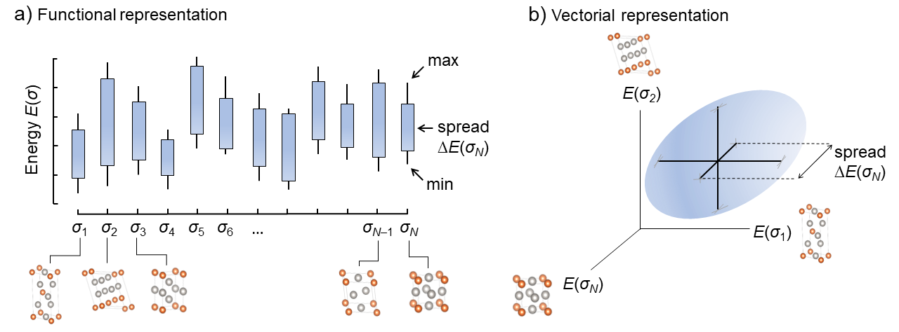
Figure 1: Functional and vectorial representations of the statistical distribution of the energies of the $N$ configurations. (a) By calculating the average and spread of the energy of each cluster across selected empirical potentials, one obtains a statistical energy distribution. (b) This distribution can be represented as a Gaussian probability in $N$-dimensional vector space.

Parameterizing cluster expansions poses two critical challenges: (i) selecting suitable crystal structures for training and (ii) controlling errors associated to the truncation of the expansion [2]. Much literature has focused on developing optimal truncation of the infinite cluster basis, as selecting the optimal training structures heavily relies on the chosen truncation approach [2, 1]. Recent advances include the integration of Bayesian methods [17, 20, 2], which enable the inclusion of physics-informed priors. These priors can significantly decrease data requirements in training cluster expansions [17]. As an example, Mueller et al. [20] extended the Bayesian approach to incorporate nonlocal, composition-dependent effects for Au–Pd nanoparticles, leading to a significant increase in efficiency compared to conventional cluster selection methods. Despite these developments, it may still be demanding to apply the cluster expansion approach to nanostructures, interfaces, and complex multicomponent mixtures due to the large dataset that must be generated from first principles [21].

Here, we develop and validate an efficient and versatile algorithm to tackle these challenges by using transfer learning to reduce the number of computationally costly calculations needed in a large configurational space. This approach exploits Bayesian inference to leverage prior knowledge from classical empirical reactive potentials, enabling the identification of the most informative configurations within the training set [22, 23, 17, 24]. We highlight the effectiveness of this approach by studying the thermodynamic stability of Pt:Ni intermetallics.

2 Methodology

2.1 Cluster expansion

Within the cluster expansion approach, the total energy $E$ of a configuration ${\boldsymbol{\sigma}}$ of a system is expressed as the sum of energies associated with symmetrically inequivalent clusters that make up that configuration [7, 25]:

$$E({\boldsymbol{\sigma}})=\sum_{\alpha}{m_{\alpha}J_{\alpha}\pi_{\alpha}({\boldsymbol{\sigma}})},$$ (1)

where $\pi_{\alpha}({\boldsymbol{\sigma}})=\left\langle\prod_{i}\varphi_{\alpha,i}(\sigma_{i})\right\rangle_{\alpha}$ represents a cluster product averaged over a collection of symmetrically inequivalent clusters labeled by the index $\alpha$ with $i$ being the site index and $(\varphi_{\alpha,i})_{\alpha}$ being a basis of orthogonal functions of the site-dependent occupation $\sigma_{i}$. Multiplicity factors ($m_{\alpha}$) quantify how many times a symmetrically equivalent cluster appears throughout the lattice and $J_{\alpha}$ is the effective cluster interaction (ECI) corresponding to the energy contribution of a cluster to the total energy.

To derive a cluster expansion, it is necessary to determine the ECIs. This process involves acquiring reference data, typically in the form of a set of configurations, along with an associated vector of target data, which is usually obtained from first-principles calculations. Equation (1) can be expressed in a simplified form as [26]

$${\boldsymbol{E}}={\boldsymbol{\Pi}}{\boldsymbol{J}},$$ (2)

where $E$ denotes the target property (typically, the energy), ${\boldsymbol{J}}$ represents the ECIs and ${\boldsymbol{\Pi}}$ is the matrix of cluster products. The ECIs can be estimated as

$${\boldsymbol{J}}={\boldsymbol{\Pi}}^{+}{\boldsymbol{E}}.$$ (3)

where ${\boldsymbol{\Pi}}^{+}\equiv({\boldsymbol{\Pi}}^{\top}{\boldsymbol{\Pi}})^{-1}{\boldsymbol{\Pi}}^{\top}$ denotes the pseudoinverse of ${\boldsymbol{\Pi}}$.

2.2 Bayesian sampling

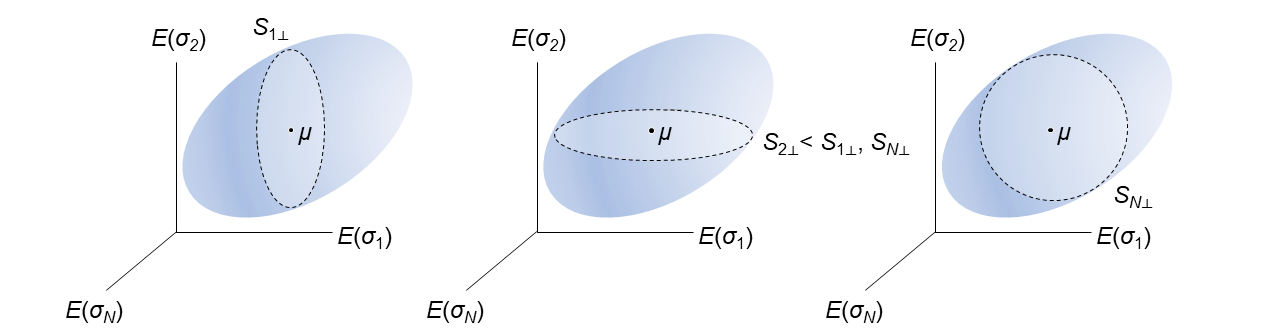
Figure 2: Evaluation of the posterior uncertainty by examining cross sections (representing the marginal probability distributions) of the prior Gaussian distribution. The uncertainty of posterior obtained by sampling configuration $\boldsymbol{\sigma}_{n}$ equals the area $S_{n\perp}$ of the associated cross section going through the mean $\boldsymbol{\mu}$ of the Gaussian distribution. The configuration to be sampled is the one minimizing the cross-sectional area (the marginal uncertainty); here, the configuration $\boldsymbol{\sigma}_{2}$.

Bayesian analysis proceeds by first specifying a prior distribution over hypotheses or parameters, representing initial beliefs. Using Bayes’ theorem, as new data becomes available, the prior is combined with the likelihood to compute the posterior distribution, which quantifies the updated beliefs. In simple terms, Bayes’ theorem can be expressed as [27]

$$\big{(}{\sf Posterior}\big{)}=\frac{{\sf\big{(}Likelihood\big{)}}\times{\sf\big{(}Prior\big{)}}}{{\sf\big{(}Marginal\;likelihood\big{)}}}.$$ (4)

This approach enables for not only parameter estimation but also offers the ability to account for uncertainty and incorporate domain knowledge effectively using Gaussian statistical distributions $\mathcal{G}$ [28]. An example of energy distribution for a collection of $N$ configurations is shown in Fig. 1. The conventional functional representation of the distribution is illustrated in Fig. 1(a). An equivalent $N$-dimensional vectorial description of the same energy distribution is shown in Fig. 1(b).

The goal of Bayesian sampling is to minimize the number of first-principles calculations by identifying a subset of configurations from a larger pool of configurations that effectively replicates the energy values. To attain this objective, the initial step involves calculating the energy of each structure using empirical potentials like COMB3 (third-generation charge optimized many-body potentials) [29], ReaxFF (reactive force fields) [30], MEAM (modified embedded-atom model) [31], EAM (embedded atom model) [32], to name a few. Reliable parameterizations exist in these potentials for the system under consideration. This process allows one to generate the Gaussian prior

$$\mathcal{G}(\boldsymbol{E})=\left|2\pi\boldsymbol{A}^{-1}\right|^{-\frac{1}{2}}\exp\left(-\frac{1}{2}(\boldsymbol{E}-\boldsymbol{\mu})^{\top}\boldsymbol{A}(\boldsymbol{E}-\boldsymbol{\mu})\right),$$ (5)

where $\boldsymbol{E}$ is a $N$-dimensional vector representing the energies of the $N$ configurations, $\boldsymbol{\mu}=\operatorname{\mathbb{E}}[\boldsymbol{E}]$ is the expectation value of $\boldsymbol{E}$, $\boldsymbol{A}=\boldsymbol{K}^{-1}$ is the inverse of the covariance matrix $\boldsymbol{K}$ , which describes the correlations between the energies ($\boldsymbol{K}=\operatorname{\mathbb{E}}[(\boldsymbol{E}-\boldsymbol{\mu})^{\top}(\boldsymbol{E}-\boldsymbol{\mu})]$), and $|\cdot|$ denotes the determinant.

To describe the sampling method, we express $\mathcal{G}(\boldsymbol{E})$ as

$$\mathcal{G}({\boldsymbol{E}})={\left|2\pi\boldsymbol{A}^{-1}\right|^{-\frac{1}{2}}}\\ \times\,{\exp{\left[-\displaystyle\frac{1}{2}\begin{pmatrix}{\boldsymbol{E}}_{\perp}-{\boldsymbol{\mu}}_{\perp}\\ {\boldsymbol{E}}_{\parallel}-{\boldsymbol{\mu}}_{\parallel}\end{pmatrix}^{\top}\begin{pmatrix}\boldsymbol{A}_{\perp\perp}&\boldsymbol{A}_{\perp\parallel}\\ \boldsymbol{A}_{\parallel\perp}&\boldsymbol{A}_{\parallel\parallel}\end{pmatrix}\begin{pmatrix}{\boldsymbol{E}}_{\perp}-{\boldsymbol{\mu}}_{\perp}\\ {\boldsymbol{E}}_{\parallel}-{\boldsymbol{\mu}}_{\parallel}\end{pmatrix}\right]}},$$ (6)

where $\parallel$ indicates the projection on the subspace of the sampled configuration and $\perp$ indicates the projection out of this subspace. The prior can then be refined via Bayesian inference using the configurations that have been sampled at the previous iterations. Using this information, Eq. (4) can be rewritten as

$$\mathcal{G}({\boldsymbol{E}}_{\perp}|{\boldsymbol{E}}_{\parallel}={\boldsymbol{E}}_{0})=\frac{\mathcal{G}({\boldsymbol{E}}_{\perp},{\boldsymbol{E}}_{0})}{\int_{\perp}{\mathcal{G}({\boldsymbol{E}}_{\perp},{\boldsymbol{E}}_{0})d{\boldsymbol{E}}_{\perp}}},$$ (7)

where $\mathcal{G}({\boldsymbol{E}}_{\perp}|{\boldsymbol{E}}_{\parallel}={\boldsymbol{E}}_{0})$ denotes the posterior distribution obtained by replacing ${\boldsymbol{E}}_{\parallel}$ with ${\boldsymbol{E}}_{0}$, which represents the energies of the already sampled configurations, $\int_{\perp}{\mathcal{G}({\boldsymbol{E}}_{\perp},{\boldsymbol{E}}_{0})d{\boldsymbol{E}}_{\perp}}$ is the marginal likelihood and $\mathcal{G}({\boldsymbol{E}}_{\perp},{\boldsymbol{E}}_{0})$ stands for the likelihood-weighted prior. Equation (7) yields

$$\mathcal{G}({\boldsymbol{E}}_{\perp}|{\boldsymbol{E}}_{\parallel}={\boldsymbol{E}}_{0})=\left|2\pi\boldsymbol{A}_{\perp\perp}^{-1}\right|^{-\frac{1}{2}}\\ \times\exp\bigg{(}-\frac{1}{2}\big{[}{\boldsymbol{E}}_{\perp}-{\boldsymbol{\mu}}_{\perp}-\boldsymbol{A}_{\perp\perp}^{-1}\boldsymbol{A}_{\perp\parallel}({\boldsymbol{E}}_{0}-{\boldsymbol{\mu}}_{\parallel})\big{]}^{\top}\\ \cdot\boldsymbol{A}_{\perp\perp}\big{[}{\boldsymbol{E}}_{\perp}-{\boldsymbol{\mu}}_{\perp}-\boldsymbol{A}_{\perp\perp}^{-1}\boldsymbol{A}_{\perp\parallel}({\boldsymbol{E}}_{0}-{\boldsymbol{\mu}}_{\parallel})\big{]}\bigg{)},$$ (8)

which can be further simplified into

$$\mathcal{G}({\boldsymbol{E}}_{\perp}|{\boldsymbol{E}}_{\parallel}={\boldsymbol{E}}_{0})=\left|2\pi{\boldsymbol{K}}_{\perp\perp}^{\prime}\right|^{-\frac{1}{2}}\\ \times\exp\left(-\frac{1}{2}({\boldsymbol{E}}_{\perp}-{\boldsymbol{\mu}}_{\perp}^{\prime})^{\top}({\boldsymbol{K}}_{\perp\perp}^{\prime})^{-1}({\boldsymbol{E}}_{\perp}-{\boldsymbol{\mu}}_{\perp}^{\prime})\right),$$ (9)

where ${\boldsymbol{\mu}}_{\perp}^{\prime}$ and ${\boldsymbol{K}}_{\perp\perp}^{\prime}$ denote the mean and the covariance of the posterior, respectively. Thus, by comparing Eqs. (8) and (9), the mean and the covariance of the posterior can be determined iteratively as

$${\boldsymbol{K}}_{n+1}=\left[({\boldsymbol{K}}_{n}^{-1})_{\perp\perp}\right]^{-1}$$ (10)

$${\boldsymbol{\mu}}_{n+1}=({\boldsymbol{\mu}}_{n})_{\perp}-{\boldsymbol{K}}_{n+1}({\boldsymbol{K}}_{n}^{-1})_{\perp\parallel}(E_{\parallel}{\boldsymbol{\sigma}}_{\parallel}-({\boldsymbol{\mu}}_{n})_{\parallel}),$$ (11)

where ${\boldsymbol{K}}_{n}$ and ${\boldsymbol{\mu}}_{n}$ are the covariance matrix and mean vector of the prior after $n$ iterations, $E_{\parallel}$ is the energy of the configuration ${\boldsymbol{\sigma}}_{\parallel}$ that has been newly sampled at the current ($n^{\rm th}$) iteration.

In Eqs. (10) and (11), the configuration ${\boldsymbol{\sigma}}_{\parallel}$ that is sampled (i.e. the configuration whose energy will be calculated at the DFT level at the next step of the iterative process) is the one that results in the largest reduction in the uncertainty of the posterior, which is represented as the area $S_{n\perp}$ of the $\boldsymbol{\mu}$-centered projection of the prior along the direction of the configuration ${\boldsymbol{\sigma}}_{n}$, as illustrated in Fig. 2. In this example, because $S_{2\perp}$ is the lowest cross-section area, the configuration ${\boldsymbol{\sigma}}_{\parallel}={\boldsymbol{\sigma}}_{2}$ will be selected, as this choice will result in maximal reduction of the posterior uncertainty. Analytically, $S_{n\perp}$ is calculated as the determinant of the covariance matrix ${\boldsymbol{K}}_{\perp\perp}={\boldsymbol{A}}^{-1}_{\perp\perp}$ after removing the row and column corresponding to that configuration from the inverse covariance matrix ${\boldsymbol{A}}$.

One of the benefits of the Bayesian approach is the ability to quantify uncertainties $\Delta E({\boldsymbol{\sigma}})$ and $\Delta J({\boldsymbol{\alpha}})$ associated to both energy predictions

$$\Delta E({\boldsymbol{\sigma}})=2\left({\boldsymbol{\sigma}}^{\top}\boldsymbol{K}_{n+1}{\boldsymbol{\sigma}}\right)^{\frac{1}{2}}$$ (12)

and cluster-expansion parameters:

$$\Delta J({\boldsymbol{\alpha}})=2\left({\boldsymbol{\alpha}}^{\top}\boldsymbol{K}_{n+1}{\boldsymbol{\alpha}}\right)^{\frac{1}{2}},$$ (13)

where $\boldsymbol{\alpha}=(\pi_{\alpha}({\boldsymbol{\sigma}}_{n}))_{n}$ is the vector representing cluster $\alpha$ across the configurational space. The step-by-step implementation of the Bayesian sampling approach is described in the supplementary information (SI). The next section presents its application and validation in predicting the stability of Pt:Ni binaries.

2.3 Simulation parameters

The Quantum-ESPRESSO suite for plane-wave materials simulations was used to perform the DFT calculations [33, 34]. Projector-augmented-wave pseudopotentials from the PseudoDojo library were selected to represent the ionic cores [35] and Perdew–Burke–Ernzerhof (PBE) [36] exchange-correlation functional was used to calculate the energies. The kinetic energy cutoffs for the plane waves expansion of wavefunctions and electronic charge density were set to 80 Ry and 320 Ry, respectively. To sample the Brillouin zone across the cells, the ${\boldsymbol{k}}$-spacing value was set to 0.025 Å^-1. Electronic occupations were smoothened using Marzari–Vanderbilt cold smearing [37], with a smearing width of 0.01 Ry. The kinetic energy cutoffs, ${\boldsymbol{k}}$-points and smearing were found to be sufficient to converge the total energies within 1 meV per atom and the forces within 1 meV/Å. Classical simulations were performed in the Large-Scale Atomic/Molecular Massively Parallel Simulator (LAMMPS) software program [38]. The interatomic potentials follow the parameterization described in Refs. [32, 31, 30, 39]. The 413 configurations were expanded to $7\times 7\times 7$ bulk supercells and then transformed to LAMMPS data files using the Atomsk software package [40].

3 Results and discussion

To illustrate the Bayesian structure selection, we considered the face-centered cubic Pt:Ni binary alloy. A database of 413 symmetrically unique configurations of Pt:Ni mixtures was produced, corresponding to all distinct supercells with up to 8 atoms using ICET software package [26, 41]. As previously stated, our objective is to decrease the number of first-principles calculations required within an extensive training set. This approach utilizes Bayesian analysis to obtain an empirical prior from interatomic potentials, facilitating the recognition of the most relevant configurations within the training set. In specific terms, we employed a total of six interatomic potentials to compute the energy of all structures in our dataset and calculate priors within the Bayesian framework. These encompassed two empirical potentials (EAM [32] and MEAM [31]), two reactive many-body potentials (COMB3 [29] and ReaxFF [30]) potentials, and two machine learning-based potentials, namely, the Crystal Hamiltonian Graph Neural Network (CHGNet) [42] and the Materials Graph Neural Network with Three-Body Interactions (M3GNet) [43]. The formation energies for the 413 structures were calculated by energy minimization in the microcanonical ensemble using the following equation:

$$\Delta E_{\rm f}=E_{{\rm Pt}_{x}{\rm Ni}_{1-x}}-xE_{\rm Pt}-(1-x)E_{\rm Ni}$$ (14)

Our approach is based on the premise that the prior is sufficiently large to include the DFT data. We systematically tested this hypothesis by comparing formation energies calculated from DFT and those computed with the interatomic potentials mentioned in the preceding paragraph. The comparison is presented using parity plots in Figure 3. As shown in Fig. 3(a), there exist significant discrepancies between the DFT and COMB3 energies. However, these discrepancies do not imply that COMB3 does carry exploitable information about the DFT energies. In fact, upon renormalizing, e.g., the COMB3 energies by the scaling factor

$$\alpha^{\rm COMB3}=\left({(\boldsymbol{E}^{\rm COMB3})^{\top}\boldsymbol{E}^{\rm COMB3}}\right)^{-1}{(\boldsymbol{E}^{\rm COMB3})^{\top}\boldsymbol{E}^{\rm DFT}}$$ (15)

(where $\boldsymbol{E}^{\rm DFT}$ represents the DFT energies and $\boldsymbol{E}^{\rm COMB3}$ is the energy calculated using COMB3 potential), a close correspondence is found between the DFT and COMB3 trends, suggesting that the ordering of the calculated COMB3 energies is qualitatively consistent with its DFT counterpart [Fig. 3(b)]. In practice, the calculation of the rescaling factor is repeated for all the interatomic potentials in each iteration, allowing for the gradual improvement of the empirical trends with the progressive incorporation of newly available DFT energies. Thus, the interatomic potentials closely capture correlations between DFT energies, as systematically demonstrated in Figs. S1 and S2 (SI).

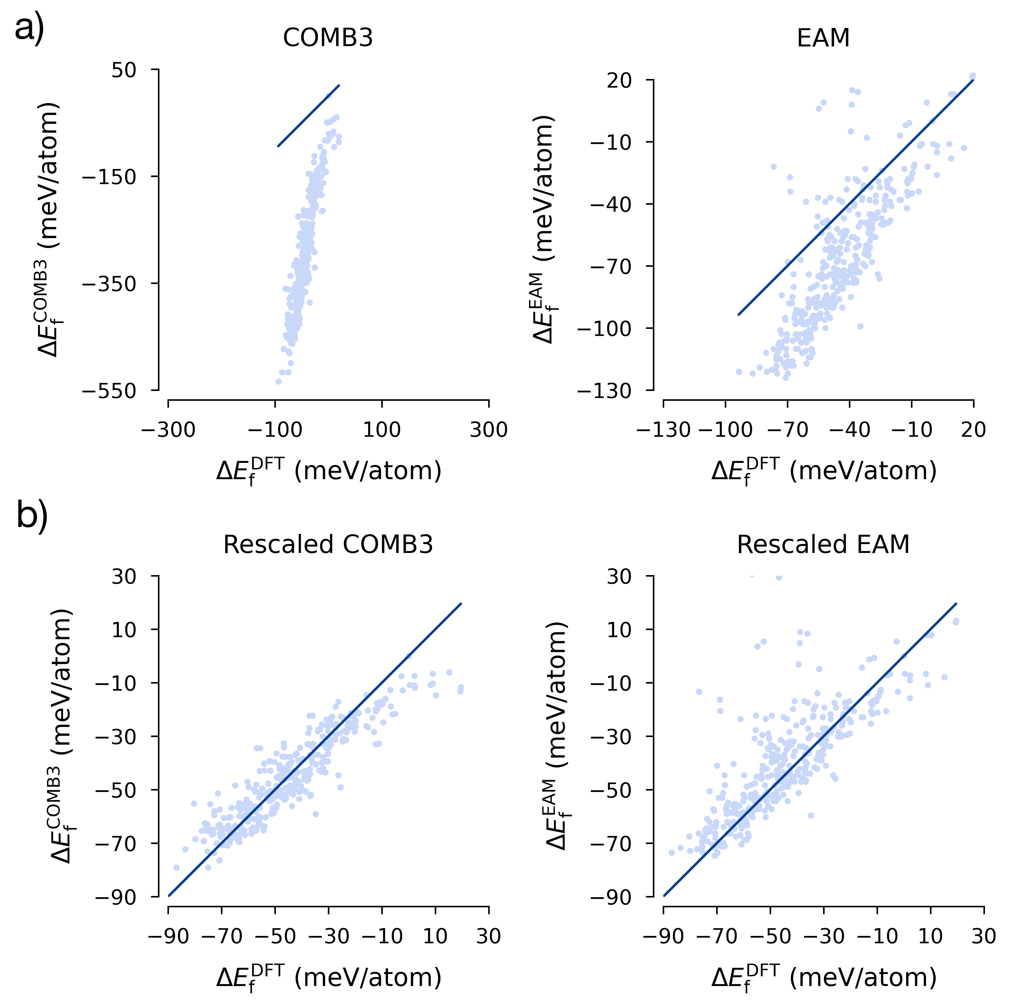
Figure 3: Parity plots between DFT energies, COMB3, and EAM (a) before scaling and (b) after scaling.

Next, a cluster expansion was parameterized, encompassing clusters up to the fourth order, with cutoff distances of 10 Å for pairs, 7.5 Å for triplets, and 5 Å for quadruplets. This cluster space was composed of a total of 130 parameters, distributed as follows: 1 zerolet, 1 singlet, 17 pairs, 76 triplets, and 35 quadruplets. To analyze how the performance of the approach is affected by increasing the number of DFT calculations in each iteration, we generated a learning curve by assessing the root mean squared error (RMSE) against a cluster expansion derived solely from DFT calculations. It should be mentioned that 370 out of the initial 413 structures were successfully converged during the DFT calculations. Structures that did not converge were excluded from our interatomic potentials database.

We derived the prior distribution by utilizing six different interatomic potentials, and this prior was employed in the iterative process of minimizing uncertainty to select the optimal configurations. The performance of the resulting Bayesian sampling method is compared to randomly sampling (uniform sampling) structures, as depicted in Fig. 4(a), which illustrates the root mean squared error of the Bayesian and random cluster expansion models with respect to a cluster expansion model solely derived from DFT calculations. A notable difference in the convergence of the RMSE is observed, especially at the initial stages of iterations where Bayesian sampling leads to an immediate decrease of the RMSE. After the 60th iteration, uniform sampling seems to outperform Bayesian sampling. However, as shown in Fig. 5(a), the convex hull generated using uniform sampling at iteration 60 noticeably differs from the convex hull created using all available training structures, while the Bayesian convex hull is already very close to its target.

To further assess the convergence of the convex hull, we introduce an alternative metric, the areal convex hull error (ACHE), obtained by calculating the area between the convex hull curves, as depicted graphically in Fig. 5(a). Changes in ACHE during the iterative cycle are reported in Fig. 4(b). A noteworthy observation is the close alignment between the Bayesian and DFT curves after 20-40 iterations, while uniform sampling requires 150-170 iterations to reach an ACHE accuracy of 3 meV. Additionally, with Bayesian sampling, the correct prediction of the convex hull is achieved after 100 iterations [Fig. 5(b)], whereas uniform sampling provides consistent predictions only after 250 iterations, Fig. 5(c). These observations demonstrate that Bayesian sampling significantly reduces the number of DFT calculations needed to build accurate cluster expansions.

It is worth emphasizing that further computational acceleration would be achieved by opting for a batch selection strategy at each iteration (as opposed to processing individual structures) and by conducting parallel DFT calculations for the selected batch. To assess the effectiveness of this approach, we conducted a test by calculating the DFT energy for 5 or 10 structures in each iteration. The results demonstrated a marginal increase in the number of DFT calculations required. With a batch of 5, the model achieved convergence after 105 DFT calculations, while for a batch of 10, convergence was attained after 110 DFT calculations [Fig. 5(d)]. In contrast, the single-structure selection approach reached convergence after 100 DFT calculations. Therefore, it is advisable to employ batch selection to maximize time savings in generating cluster expansions.

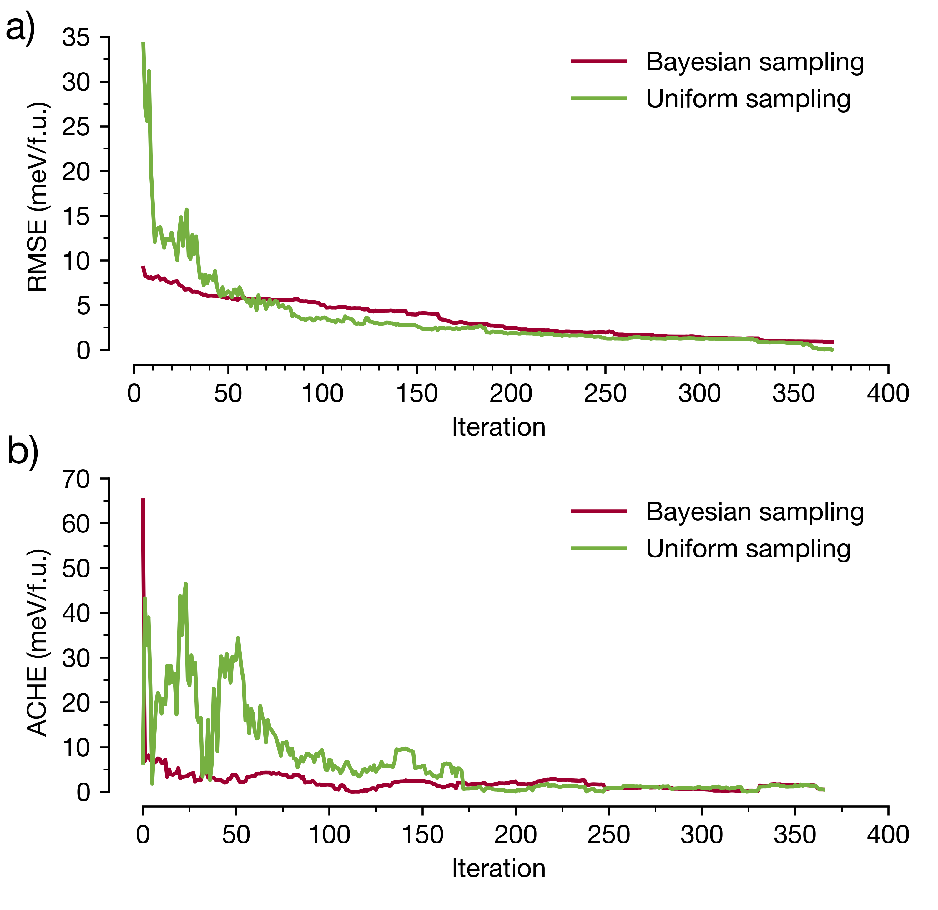
Figure 4: Construction of a cluster expansion using Bayesian and uniform sampling. (a) RMSE for each iteration is obtained against a cluster expansion derived from 370 DFT calculations. (b) Areal convex hull error (ACHE) between the Bayesian sampling and DFT, and uniform sampling and DFT as function of the number of iterations.

Figure 5: Cluster expansion performance at different iterations. The concentrations corresponding to cluster expansion energies obtained from uniform (Bayesian) sampling are slightly shifted to the right (left) of the actual concentrations, to evidence their deviations from the DFT energies. Convex hull diagrams after (a) 60 iterations, (b) 100 iterations, and (c) 250 iterations. (d) Convex hull plots after 11 iterations of batch sampling, whereby 10 DFT calculations are performed in parallel at each iteration. The areal convex hull errors (ACHEs) are shown as the colored (red and green) transparent regions in panel (a) (for Bayesian and uniform sampling, respectvely).

4 Conclusion

We introduced a Bayesian selection algorithm to efficiently construct cluster expansions from minimal DFT inputs. This algorithm optimizes the selection of DFT-computed structures for the cluster expansion and can be seamlessly integrated with any cluster expansion method to maximize model accuracy while minimizing computational cost.

We demonstrated the practical applicability of this method using empirical potentials to generate a Gaussian prior. This prior enables one to identify the most informative structures within a training set for model construction. The energies of these selected structures are then calculated at the DFT level. Subsequently, the prior is updated by incorporating the DFT energies, and new structures are chosen for the next iteration. This iterative process continues until a cluster expansion model with sufficient RMSE (root mean squared error) and ACHE (areal convex hull error) accuracy is achieved.

Applying this approach to a prototypical Pt:Ni alloy yields a reduction in computational cost by a factor of $\sim$2.5 compared with uniform sampling. Importantly, this reduction did not compromise the robust convergence of cluster expansions; to the contrary, much lower statistical fluctuations were observed when applying Bayesian sampling. Further computational acceleration is attained by selecting a batch of structures at each iteration rather than performing DFT calculations for single structures. This algorithm provides a promising approach for future studies of electrochemical interfaces under applied voltage and multicomponent materials at finite temperature.

5 Acknowledgments

This work was primarily supported by the U.S. Department of Energy, Office of Science, Basic Energy Sciences, CPIMS (Condensed Phase and Interfacial Molecular Science) Program, under Award No. DE-SC0018646. S.G. acknowledges support from the Center for Nanoscale Science under Grant No. DMR-2011839 (code implementation, code validation, and development of accuracy metrics). I.D. and A.D. are thankful to Paul E. Lammert for fruitful discussions on the analytical foundations of the cluster expansion method.

References

- [1] Sara Kadkhodaei and Jorge A Muñoz. Cluster expansion of alloy theory: a review of historical development and modern innovations. JOM, 73(11):3326–3346, 2021.
- [2] Nelson, Lance J and Ozoliņš, Vidvuds and Reese, C Shane and Zhou, Fei and Hart, Gus LW. Cluster expansion made easy with Bayesian compressive sensing. Physical Review B, 88(15):155105, 2013.
- [3] C Wolverton and Alex Zunger. Prediction of Li Intercalation and Battery Voltages in Layered vs. Cubic LixCoO2. Journal of The Electrochemical Society, 145(7):2424, 1998.
- [4] Atsuto Seko, Koretaka Yuge, Fumiyasu Oba, Akihide Kuwabara, and Isao Tanaka. Prediction of ground-state structures and order-disorder phase transitions in II-III spinel oxides: A combined cluster-expansion method and first-principles study. Physical Review B, 73(18):184117, 2006.
- [5] Brian Kolb and Gus LW Hart. Nonmetal ordering in TiC1-xNx: Ground-state structure and the effects of finite temperature. Physical Review B, 72(22):224207, 2005.
- [6] Adam Carlsson, Johanna Rosen, and Martin Dahlqvist. Finding stable multi-component materials by combining cluster expansion and crystal structure predictions. npj Computational Materials, 9(1):21, 2023.
- [7] Qu Wu, Bing He, Tao Song, Jian Gao, and Siqi Shi. Cluster expansion method and its application in computational materials science. Computational Materials Science, 125:243–254, 2016.
- [8] V Ozoliņš, C Wolverton, and Alex Zunger. Cu-Au, Ag-Au, Cu-Ag, and Ni-Au intermetallics: First-principles study of temperature-composition phase diagrams and structures. Physical Review B, 57(11):6427, 1998.
- [9] JM Sanchez, JL Moran-Lopez, C Leroux, and MC Cadeville. Magnetic properties and chemical ordering in Co-Pt. Journal of Physics: Condensed Matter, 1(2):491, 1989.
- [10] Mark Asta, Ryan McCormack, and Didier de Fontaine. Theoretical study of alloy phase stability in the Cd-Mg system. Physical Review B, 48(2):748, 1993.
- [11] A Van der Ven and G Ceder. Vacancies in ordered and disordered binary alloys treated with the cluster expansion. Physical Review B, 71(5):054102, 2005.
- [12] Liang Cao, Chenyang Li, and Tim Mueller. The use of cluster expansions to predict the structures and properties of surfaces and nanostructured materials. Journal of chemical information and modeling, 58(12):2401–2413, 2018.
- [13] Axel van de Walle and Gerbrand Ceder. Automating first-principles phase diagram calculations. Journal of Phase Equilibria, 23(4):348, 2002.
- [14] Atsuto Seko, Yukinori Koyama, and Isao Tanaka. Cluster expansion method for multicomponent systems based on optimal selection of structures for density-functional theory calculations. Physical Review B, 80(16):165122, 2009.
- [15] Tim Mueller and Gerbrand Ceder. Exact expressions for structure selection in cluster expansions. Physical Review B, 82(18):184107, 2010.
- [16] Eric Cockayne and Axel van de Walle. Building effective models from sparse but precise data: Application to an alloy cluster expansion model. Physical Review B, 81(1):012104, 2010.
- [17] Tim Mueller and Gerbrand Ceder. Bayesian approach to cluster expansions. Physical Review B, 80(2):024103, 2009.
- [18] Lance J Nelson, Gus LW Hart, Fei Zhou, Vidvuds Ozoliņš, et al. Compressive sensing as a paradigm for building physics models. Physical Review B, 87(3):035125, 2013.
- [19] Robert Tibshirani. Regression shrinkage and selection via the lasso. Journal of the Royal Statistical Society Series B: Statistical Methodology, 58(1):267–288, 1996.
- [20] Tim Mueller. Ab initio determination of structure-property relationships in alloy nanoparticles. Physical Review B, 86(14):144201, 2012.
- [21] Tatiana Kostiuchenko, Fritz Körmann, Jörg Neugebauer, and Alexander Shapeev. Impact of lattice relaxations on phase transitions in a high-entropy alloy studied by machine-learning potentials. npj Computational Materials, 5(1):55, 2019.
- [22] Carl Edward Rasmussen. Gaussian processes in machine learning. In Summer school on machine learning, pages 63–71. Springer, 2003.
- [23] Daniel Packwood et al. Bayesian optimization for materials science. Springer, 2017.
- [24] Milica Todorović, Michael U Gutmann, Jukka Corander, and Patrick Rinke. Bayesian inference of atomistic structure in functional materials. Npj computational materials, 5(1):35, 2019.
- [25] JM Sanchez and T Mohri. Approximate solutions to the cluster variation free energies by the variable basis cluster expansion. Computational Materials Science, 122:301–306, 2016.
- [26] Mattias Ångqvist, William A Muñoz, J Magnus Rahm, Erik Fransson, Céline Durniak, Piotr Rozyczko, Thomas H Rod, and Paul Erhart. ICET–a Python library for constructing and sampling alloy cluster expansions. Advanced Theory and Simulations, 2(7):1900015, 2019.
- [27] Carl Edward Rasmussen, Christopher KI Williams, et al. Gaussian processes for machine learning, volume 1. Springer, 2006.
- [28] Andrew Gelman, John B Carlin, Hal S Stern, and Donald B Rubin. Bayesian data analysis. Chapman and Hall/CRC, 1995.
- [29] Tao Liang, Tzu Ray Shan, Yu Ting Cheng, Bryce D. Devine, Mark Noordhoek, Yangzhong Li, Zhize Lu, Simon R. Phillpot, and Susan B. Sinnott. Classical atomistic simulations of surfaces and heterogeneous interfaces with the charge-optimized many body (COMB) potentials, 2013.
- [30] Yun Kyung Shin, Lili Gai, Sumathy Raman, and Adri C.T. Van Duin. Development of a ReaxFF Reactive Force Field for the Pt-Ni Alloy Catalyst. Journal of Physical Chemistry A, 120(41):8044–8055, 10 2016.
- [31] Jin-Soo Kim, Donghyuk Seol, Joonho Ji, Hyo-Sun Jang, Yongmin Kim, and Byeong-Joo Lee. Second nearest-neighbor modified embedded-atom method interatomic potentials for the Pt-M (M = Al, Co, Cu, Mo, Ni, Ti, V) binary systems. Calphad, 59:131–141, 12 2017.
- [32] S M Foiles, M I Baskes, and M S Daw. Embedded-atom-method functions for the fcc metals Cu, Ag, Au, Ni, Pd, Pt, and their alloys. Physical Review B, 33(12):7983–7991, 6 1986.
- [33] Paolo Giannozzi, Stefano Baroni, Nicola Bonini, Matteo Calandra, Roberto Car, Carlo Cavazzoni, Davide Ceresoli, Guido L Chiarotti, Matteo Cococcioni, Ismaila Dabo, et al. QUANTUM ESPRESSO: a modular and open-source software project for quantum simulations of materials. Journal of physics: Condensed matter, 21(39):395502, 2009.
- [34] Paolo Giannozzi, Oliviero Andreussi, Thomas Brumme, Oana Bunau, M Buongiorno Nardelli, Matteo Calandra, Roberto Car, Carlo Cavazzoni, Davide Ceresoli, Matteo Cococcioni, et al. Advanced capabilities for materials modelling with Quantum ESPRESSO. Journal of physics: Condensed matter, 29(46):465901, 2017.
- [35] François Jollet, Marc Torrent, and Natalie Holzwarth. Generation of Projector Augmented-Wave atomic data: A 71 element validated table in the XML format. Computer Physics Communications, 185(4):1246–1254, 2014.
- [36] John P Perdew, Kieron Burke, and Matthias Ernzerhof. Generalized gradient approximation made simple. Physical review letters, 77(18):3865, 1996.
- [37] Nicola Marzari, David Vanderbilt, Alessandro De Vita, and MC Payne. Thermal contraction and disordering of the Al (110) surface. Physical review letters, 82(16):3296, 1999.
- [38] Steve Plimpton. Fast Parallel Algorithms for Short-Range Molecular Dynamics. Journal of Computational Physics, 117(1):1–19, 3 1995.
- [39] Jackelyn A. Martinez, Aleksandr Chernatynskiy, Dundar E. Yilmaz, Tao Liang, Susan B. Sinnott, and Simon R. Phillpot. Potential Optimization Software for Materials (POSMat). Computer Physics Communications, 203:201–211, 6 2016.
- [40] Pierre Hirel. Atomsk: A tool for manipulating and converting atomic data files. Computer Physics Communications, 197:212–219, 12 2015.
- [41] Gus LW Hart and Rodney W Forcade. Algorithm for generating derivative structures. Physical Review B, 77(22):224115, 2008.
- [42] Bowen Deng, Peichen Zhong, KyuJung Jun, Janosh Riebesell, Kevin Han, Christopher J. Bartel, and Gerbrand Ceder. CHGNet: Pretrained universal neural network potential for charge-informed atomistic modeling. 2 2023.
- [43] Chi Chen and Shyue Ping Ong. A Universal Graph Deep Learning Interatomic Potential for the Periodic Table. 2 2022.