Interpretable Graph Anomaly Detection using Gradient Attention Maps

Abstract

Detecting unusual patterns in graph data is a crucial task in data mining. However, existing methods often face challenges in consistently achieving satisfactory performance and lack interpretability, which hinders our understanding of anomaly detection decisions. In this paper, we propose a novel approach to graph anomaly detection that leverages the power of interpretability to enhance performance. Specifically, our method extracts an attention map derived from gradients of graph neural networks, which serves as a basis for scoring anomalies. In addition, we conduct theoretical analysis using synthetic data to validate our method and gain insights into its decision-making process. To demonstrate the effectiveness of our method, we extensively evaluate our approach against state-of-the-art graph anomaly detection techniques. The results consistently demonstrate the superior performance of our method compared to the baselines.

1 Introduction

Anomaly detection tasks typically focus on identifying outlier data points within a feature space, which can sometimes neglect the crucial relational information inherent in real-world data. Conversely, graphs are frequently used to capture and represent structural and relational information, introducing the concept of graph anomaly detection (GAD) [1]. GAD extends the anomaly detection paradigm to the realm of graphs, aiming to pinpoint abnormal elements within a graph, such as nodes, edges, and subgraphs, or even to identify anomalous entire graphs within a dataset or database [2]. This transition from traditional anomaly detection to GAD is illustrated in Fig. 1.

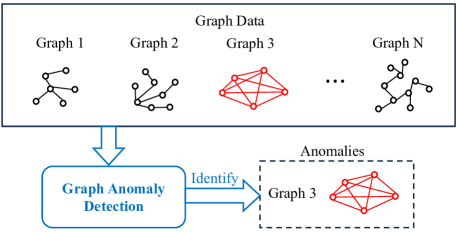
Figure 1: Illustration of graph anomaly detection (GAD) tasks.

Recent deep-learning based approaches [3, 4, 5, 6, 7, 8, 9, 10] face challenges in effectively addressing the GAD problem because of the complex relational dependencies and irregular structures associated with graph data. Nevertheless, the recent advent of geometric deep learning and graph neural networks (GNNs) has generated significant interest in utilizing these advanced methods for GAD [11] because GNNs can effectively capture comprehensive information from graph structures and node attributes. GNN-based approaches to GAD typically involve learning representations for normal graph data or normal graph elements, followed by subsequent processing for anomaly detection. One common approach in learning representations for GAD is through the use of autoencoders. For instance, GCNAE [12], DOMINANT [13], and CONAD [14] utilize GNNs to construct autoencoders and use reconstruction errors to calculate anomaly scores for nodes. Another approach is to directly output representations using neural networks. For instance, OC-GNN [15] embeds graph data into a vector space and forms a hyperplane using normal data.

However, these GAD methods are based on neural networks and are often regarded as black-box models. This lack of interpretability may hinder end users, who rely on these results to make informed decisions. In addition, the effectiveness of GNN-based GAD methods may vary across different datasets, especially because of the complex relations and heterogeneity in graph data. To address these limitations, we propose a novel approach to GAD based on GNN interpretation in this work. Our method derives anomaly scores from gradient attention maps of GNNs, and we name it accordingly as “GRAM” (an abbreviation of “GRadient Attention Map”). Our method is designed for the unsupervised GAD task where the underlying GNNs are trained solely on normal graph data. In this case, the trained GNNs only capture characteristics of normal graphs. Therefore, anomalous graph elements will exhibit distinctive highlighted regions when we examine the gradient maps of the entire graph representation with respect to node feature embeddings. Our GRAM model is based on gradient attention maps similar to a graph Grad-CAM, but the way it computes and utilizes gradients is different from [16, 17]. Furthermore, GRAM is proposed for the specific task of GAD, distinguishing it from the aforementioned works which focus on explaining the behavior of GNNs.

2 Proposed Method

For a graph ${\mathcal{G}}$ with $N$ nodes, suppose that its adjacency matrix is given by ${\mathbf{A}}\in\mathbb{R}^{N\times N}$ and its node feature matrix is given by ${\mathbf{X}}\in\mathbb{R}^{N\times M}$ where each row of ${\mathbf{X}}$ represents a $M$-dimensional node feature. Suppose that a GNN model takes ${\mathbf{X}}$ as input and produces $J$-dimensional output features as

$$\mathbf{H}=\text{GNN}\left(\mathbf{X},\mathbf{A}\right).$$ (1)

The output ${\mathbf{H}}\in\mathbb{R}^{N\times J}$ is then post-processed to produce an $I$-dimensional vector ${\mathbf{z}}\in\mathbb{R}^{I}$. For instance, in our applications, ${\mathbf{z}}$ can be computed from the latent distribution of a variational autoencoder. Our GRAM method leverages the gradients of ${\mathbf{z}}$ with respect to ${\mathbf{H}}$. Specifically, we define the gradient attention coefficients as follows:

$$\bm{\alpha}_{i}:=\frac{1}{N}\sum_{n=1}^{N}\frac{\partial z_{i}}{\partial{\mathbf{h}}_{n}}\in\mathbb{R}^{J},~{}i=1,\cdots,I,$$ (2)

where $z_{i}\in\mathbb{R}$ represents the $i$-th element of $\mathbf{z}$ and ${\mathbf{h}}_{n}\in\mathbb{R}^{J}$ represents (the transpose of) the $n$-th row of ${\mathbf{H}}$, corresponding to the $n$-th node. Next, we calculate the node-level anomaly scores for individual nodes as follows:

$$\mathbf{s}\equiv[s_{n}]_{n=1}^{N}:=\left[\sum_{i=1}^{I}\phi(\bm{\alpha}_{i}^{\textup{T}}{\mathbf{h}}_{n})\right]_{n=1}^{N},$$ (3)

where $\phi$ refers to the nonlinear activation function used for producing ${\mathbf{z}}$. The graph-level anomaly score is then given by

$$\operatorname{score}:=\operatorname{GlobalAddPooling}({\mathbf{s}})\equiv\sum_{n=1}^{N}s_{n}.$$ (4)

These anomaly scores are then thresholded to determine whether individual nodes or the entire graph are classified as anomalous. The rationale behind thresholding the anomaly scores is as follows: the underlying GNN model for producing ${\mathbf{z}}$ is trained on normal graph data, which means that it is easier for normal nodes or graphs to explain ${\mathbf{z}}$ than anomalous nodes or graphs. Consequently, when examining the attention maps, anomalies are expected to exhibit significantly different scores. This will be further validated in Section 3.

In our setting, the dataset comprises a category of normal graphs and a category of anomalous graphs. Our goal is to accurately distinguish between normal and anomalous graphs. To address this graph-level task, we employ a variational graph autoencoder (VGAE) model similar to [12], but with a different architecture, to extract graph-level features and utilize the GRAM method for anomaly detection.

In the training phase, the VGAE is trained to minimize the unsupervised graph reconstruction error and the KL-loss. The encoder consists of a GNN and two multilayer perceptron (MLP) networks. The GNN is used to extract features from the input graph data consisting of the pair $\left(\mathbf{X},\mathbf{A}\right)$ and generate the embedding $\mathbf{H}$. Then, the MLP networks generate the mean ${\mathbf{M}}$ and logarithmic standard deviation $\log\bm{\Sigma}$ for the latent variable $\mathbf{Z}$. Subsequently, the decoder consists of two MLPs and two GNNs, which decode and reconstruct the node features $\mathbf{X}$ and the adjacency matrix $\mathbf{A}$, respectively, resulting in $\tilde{\mathbf{X}}$ and $\tilde{\mathbf{A}}$. The reconstruction error is calculated by comparing the reconstructed $\tilde{\mathbf{X}}$ and $\tilde{\mathbf{A}}$ with the original input $\mathbf{X}$ and $\mathbf{A}$. The total loss for the VGAE is thus

$$\beta\left\|\mathbf{X}-\tilde{\mathbf{X}}\right\|_{\rm F}^{2}+\left(1-\beta\right)\left\|\mathbf{A}-\tilde{\mathbf{A}}\right\|_{\rm F}^{2}+\text{KL-loss},$$ (5)

where $\beta$ is a hyperparameter, $\left\|\cdot\right\|_{\rm F}$ is the Frobenius norm, and the KL-loss is computed by

KL-loss $$=-\frac{1}{2N}(\mathbf{1}_{N})^{\textup{T}}\Big{[}(\mathbf{1}_{N})(\mathbf{1}_{M})^{\textup{T}}+2\log\bm{\Sigma}$$ (6)

$$\qquad-{\mathbf{M}}\odot{\mathbf{M}}-\exp({2\log\bm{\Sigma}})\Big{]}(\mathbf{1}_{M}).$$

Here, $\mathbf{1}_{N}$ and $\mathbf{1}_{M}$ represent column vectors of all ones, with dimensions $N$ and $M$ respectively. Moreover, $\odot$ represents pointwise multiplication.

In the testing phase, the trained encoder is utilized to produce the vector ${\mathbf{z}}$ for each test graph, which is derived by applying global add pooling to $\mathbf{Z}$. Then, the latent vector $\mathbf{z}$ is used to calculate the anomaly score according to (2)–(4).

3 Analysis on a Simple Scenario

To gain insights into the regime and validate the effectiveness of GRAM, we conduct the following theoretical analysis. We consider a synthetic graph dataset which consists of two distinct types of graphs: tree-structured graphs and double ring-structured graphs, where each graph has $N$ nodes. In Fig. 2, we show two examples of graph data that fall in the above two categories. The left is a binary tree graph, and the right is a double ring graph. Both graphs consist of $7$ nodes but are of clearly different structures.

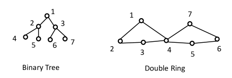
Figure 2: Examples of a binary tree graph and a double ring graph.

According to our proposed method described in Section 2, we use GRAM based on the VGAE model to address this task. For simplicity, throughout this paper, we employ the graph convolutional network (GCN) [18] as the underlying architecture for our GNN, which enables efficient feature propagation along graph edges. Specifically, we consider a GCN with $L=4$ layers, where the message passing operation in the $l$-th layer of GCN is represented as

$$\mathbf{H}^{(l+1)}=\mathbf{\hat{D}}^{-\frac{1}{2}}\mathbf{\hat{A}}\mathbf{\hat{D}}^{-\frac{1}{2}}\mathbf{H}^{(l)}\mathbf{W}^{(l)},~{}l=0,1,2,3.$$ (7)

Here, $\mathbf{\hat{A}}=\mathbf{A}+\mathbf{I}$ denotes the adjacency matrix with inserted self-loops, $\mathbf{\hat{D}}$ refers to its corresponding diagonal degree matrix, and $\mathbf{W}^{(l)}$ represents the learnable parameters of the $l$-th layer. In addition, $\mathbf{H}^{(0)}=\mathbf{X}$ is the input feature and the output feature $\mathbf{H}=\mathbf{H}^{(L)}$. To facilitate theoretical analysis, we assume very simple neural network structures with no nonlinear activations between GCN layers. Nevertheless, we employ the rectified linear unit (ReLU), which has been shown to facilitate effective learning in various graph deep learning tasks, as the nonlinear activation function for the subsequent MLPs. Specifically, let the MLP networks consist of two linear layers with a ReLU activation in the middle. It generates the mean ${\mathbf{M}}$ and logarithmic standard deviation $\log\bm{\Sigma}$ as follows:

$${\mathbf{M}} =\text{MLP}_{1}(\mathbf{H})=\text{Linear}(\text{ReLU}(\text{Linear}(\mathbf{H}))),$$ (8)

$$\log\bm{\Sigma} =\text{MLP}_{2}(\mathbf{H})=\text{Linear}(\text{ReLU}(\text{Linear}(\mathbf{H}))).$$ (9)

We denote $\mathbf{W}_{\mu 1}$ and $\mathbf{W}_{\mu 2}$ as the weight matrices in the Linear layers in (8), and $\mathbf{b}_{\mu 1}$ and $\mathbf{b}_{\mu 2}$ the bias terms. Similarly, we denote $\mathbf{W}_{\sigma 1}$ and $\mathbf{W}_{\sigma 2}$ as the weight matrices of the Linear layers in (9), and $\mathbf{b}_{\sigma 1}$ and $\mathbf{b}_{\sigma 2}$ the bias terms. With the mean and logarithmic standard deviation, the latent code is then sampled according to

$$\mathbf{Z}={\mathbf{M}}+{\mathbf{E}}\odot\exp(\log\bm{\Sigma}),$$ (10)

where ${\mathbf{E}}$ is a white noise whose entries follow the standard normal distribution independently. The latent vector $\mathbf{z}$ is obtained from ${\mathbf{Z}}$ by performing global add pooling. Therefore, the gradient of $\mathbf{z}$ with respect to $\mathbf{H}$ is

$$\frac{\partial z_{i}}{\partial\mathbf{H}} =\frac{\partial z_{i}}{\partial\mathbf{Z}}\frac{\partial\mathbf{Z}}{\partial{\mathbf{M}}}\frac{\partial{\mathbf{M}}}{\partial\mathbf{H}}+\frac{\partial z_{i}}{\partial\mathbf{Z}}\frac{\partial\mathbf{Z}}{\partial\log\bm{\Sigma}}\frac{\partial\log\bm{\Sigma}}{\partial\mathbf{H}}+\frac{\partial z_{i}}{\partial\mathbf{Z}}\frac{\partial\mathbf{Z}}{\partial{\mathbf{E}}}\frac{\partial{\mathbf{E}}}{\partial\mathbf{H}}$$ (11)

$$=\frac{\partial z_{i}}{\partial\mathbf{Z}}\frac{\partial{\mathbf{M}}}{\partial\mathbf{H}}+\frac{\partial z_{i}}{\partial\mathbf{Z}}({\mathbf{E}}\odot\exp\{\log\bm{\Sigma}\})\frac{\partial\log\bm{\Sigma}}{\partial\mathbf{H}}$$

$$=(\mathbf{1}_{N})(\mathbf{e}_{i})^{\textup{T}}\Big{[}\mathbf{W}_{\mu 2}^{\textup{T}}\text{ReLU}^{\prime}(\mathbf{H}\mathbf{W}_{\mu 1}\oplus\mathbf{b}_{\mu 1})\mathbf{W}_{\mu 1}^{\textup{T}}+({\mathbf{E}}$$

$$\quad\odot\exp\{\log\bm{\Sigma}\})\mathbf{W}_{\sigma 2}^{\textup{T}}\text{ReLU}^{\prime}(\mathbf{H}\mathbf{W}_{\sigma 1}\oplus\mathbf{b}_{\sigma 1})\mathbf{W}_{\sigma 1}^{\textup{T}}\Big{]},$$

where, to simplify the representation, we abuse the notation and use ${\mathbf{H}}$, ${\mathbf{Z}}$, ${\mathbf{M}}$, $\bm{\Sigma}$, ${\mathbf{E}}$ to represent their vectorized versions.

To facilitate our analysis, we assume that in both the GCN layers and the MLP layers, the weight matrices are set as the identity matrix and the bias terms are set as zero vectors. In this case, the arguments of ReLU in (11) are nonnegative. In addition, for the synthetic graph data we consider, we use the adjacency matrix of each graph as its node feature matrix. According to our assumptions,

$${\mathbf{H}}^{(l)}=(\mathbf{\hat{D}}^{-\frac{1}{2}}\mathbf{\hat{A}}\mathbf{\hat{D}}^{-\frac{1}{2}})^{l}\mathbf{A},~{}l=1,\dots,4.$$ (12)

The $(n,j)$-th element of $\mathbf{H}={\mathbf{H}}^{(4)}\in\mathbb{R}^{N\times N}$ ($N=I=J$ following our assumption) is thus calculated as follows:

$$h_{nj} =\sum\limits_{k_{1}=1}^{N}\sum\limits_{k_{2}=1}^{N}\sum\limits_{k_{3}=1}^{N}\sum\limits_{k_{4}=1}^{N}\frac{\hat{a}_{nk_{1}}\hat{a}_{k_{1}k_{2}}\hat{a}_{k_{2}k_{3}}\hat{a}_{k_{3}k_{4}}a_{k_{4}j}}{\sqrt{\hat{d}_{n}}\hat{d}_{k_{1}}\hat{d}_{k_{2}}\hat{d}_{k_{3}}\sqrt{\hat{d}_{k_{4}}}},$$ (13)

where $\hat{a}$, $a$, and $\hat{d}$ are the elements of $\mathbf{\hat{A}}$, $\mathbf{A}$, and $\mathbf{\hat{D}}$, respectively. Moreover, (2) simplifies as follows:

$$\bm{\alpha}_{i}^{\textup{T}} =\frac{1}{N}\mathbf{1}_{N}^{\textup{T}}\Big{[}\mathbf{1}_{N}\mathbf{e}_{i}^{\textup{T}}+\mathbf{1}_{N}\mathbf{e}_{i}^{\textup{T}}{\mathbf{E}}\odot\exp\{\log\bm{\Sigma}\}\Big{]},$$ (14)

where, ${\mathbf{E}}$ follows the centered Gaussian distribution ${\mathcal{N}}(0,\epsilon{\mathbf{I}})$ and therefore $\bm{\alpha}_{i}$ is also random with

$$\bm{\alpha}_{i}=\begin{bmatrix}{\mathcal{N}}\left(0,\epsilon e^{h_{i1}}\right)\cdots{\mathcal{N}}\left(1,\epsilon e^{h_{ii}}\right)\cdots{\mathcal{N}}\left(0,\epsilon e^{h_{iN}}\right)\end{bmatrix},$$ (15)

where for simplicity we replace the random variables directly with the respective Gaussian distributions. Set $\bm{\alpha}=\sum\limits_{i=1}^{I}\bm{\alpha}_{i}$. Combining (15), (3) and (4) yields

$$\operatorname{score} =\sum_{n=1}^{N}s_{n}=\mathbf{1}_{N}^{\textup{T}}\mathbf{H}\bm{\alpha}$$ (16)

$$={\mathcal{N}}\Bigg{(}\sum_{i=1}^{N}\sum_{j=1}^{N}h_{ij},\epsilon\sqrt{\sum_{i=1}^{N}\left(\sum_{j=1}^{N}h_{ij}\right)^{2}\sum_{n=1}^{N}e^{2h_{ni}}}\Bigg{)}.$$

To apply the above analysis to our synthetic data, we calculate the node-level and graph-level scores for the two graphs in Fig. 2, showing the results corresponding to $\epsilon=0.1$ in Table 1.

Table 1: Node-level and graph-level scores obtained from the GRAM method for the two graphs in Fig. 2

	Binary tree	Double ring
Node 1	${\mathcal{N}}(1.94,0.30)$	${\mathcal{N}}(2.23,0.36)$
Node 2	${\mathcal{N}}(2.23,0.37)$	${\mathcal{N}}(2.24,0.36)$
Node 3	${\mathcal{N}}(2.23,0.37)$	${\mathcal{N}}(2.23,0.36)$
Node 4	${\mathcal{N}}(1.56,0.28)$	${\mathcal{N}}(2.91,0.45)$
Node 5	${\mathcal{N}}(1.56,0.28)$	${\mathcal{N}}(2.23,0.36)$
Node 6	${\mathcal{N}}(1.56,0.28)$	${\mathcal{N}}(2.24,0.36)$
Node 7	${\mathcal{N}}(1.56,0.28)$	${\mathcal{N}}(2.23,0.36)$
score	${\mathcal{N}}(12.65,1.74)$	${\mathcal{N}}(16.32,2.34)$

Table 2: AUC results for graph-level anomaly detection (numbers in percentage)

	MUTAG	NCI1	PROTEINS	PTC	IMDB-B	RDT-B	IMDB-M	RDT-M5K	Synthetic data
GCNAE	$79.97_{\pm 0.8}$	$62.27_{\pm 0.2}$	$72.30_{\pm 0.0}$	$\bf{{\color[rgb]{0,1,0}66.67_{\pm 0.0}}}$	$56.99_{\pm 8.8}$	$91.28_{\pm 0.1}$	$\bf{{\color[rgb]{0,1,0}59.35_{\pm 0.0}}}$	$\bf{{\color[rgb]{0,0,1}95.06_{\pm 0.1}}}$	$91.85_{\pm 5.1}$
DOMINANT	$85.61_{\pm 1.2}$	$65.36_{\pm 0.1}$	$\bf{{\color[rgb]{0,1,0}75.01_{\pm 0.1}}}$	$62.22_{\pm 0.0}$	$67.40_{\pm 2.7}$	$94.72_{\pm 0.2}$	$51.71_{\pm 2.0}$	$89.96_{\pm 0.1}$	$\bf{{\color[rgb]{0,1,0}97.72_{\pm 0.3}}}$
CONAD	$85.61_{\pm 1.2}$	$\bf{{\color[rgb]{0,1,0}65.43_{\pm 0.1}}}$	$74.96_{\pm 0.0}$	$62.22_{\pm 0.0}$	$\bf{{\color[rgb]{0,1,0}68.36_{\pm 0.9}}}$	$94.30_{\pm 0.2}$	$55.34_{\pm 0.0}$	$90.20_{\pm 0.4}$	$\bf{{\color[rgb]{0,1,0}97.72_{\pm 0.3}}}$
GAAN	$84.45_{\pm 1.6}$	$64.46_{\pm 0.0}$	$72.41_{\pm 0.0}$	$60.89_{\pm 0.0}$	$63.91_{\pm 1.1}$	$\bf{{\color[rgb]{0,0,1}97.12_{\pm 0.0}}}$	$54.12_{\pm 0.0}$	$88.26_{\pm 0.0}$	$93.27_{\pm 0.3}$
OC-GNN	$\bf{{\color[rgb]{0,0,1}88.59_{\pm 0.3}}}$	$59.30_{\pm 6.6}$	$74.54_{\pm 1.1}$	$58.22_{\pm 0.5}$	$61.97_{\pm 7.2}$	$94.16_{\pm 1.0}$	$54.71_{\pm 6.2}$	$73.73_{\pm 16.0}$	$95.06_{\pm 1.9}$
GRAM	$\bf{{\color[rgb]{0,1,0}86.99_{\pm 1.7}}}$	$\bf{{\color[rgb]{0,0,1}68.31_{\pm 0.3}}}$	$\bf{{\color[rgb]{0,0,1}76.66_{\pm 0.1}}}$	$\bf{{\color[rgb]{0,0,1}76.15_{\pm 2.9}}}$	$\bf{{\color[rgb]{0,0,1}70.76_{\pm 1.4}}}$	$\bf{{\color[rgb]{0,1,0}94.95_{\pm 0.8}}}$	$\bf{{\color[rgb]{0,0,1}61.76_{\pm 1.0}}}$	$\bf{{\color[rgb]{0,1,0}94.26_{\pm 2.1}}}$	$\bf{{\color[rgb]{0,0,1}99.49_{\pm 0.2}}}$

Table 3: AP results for graph-level anomaly detection (numbers in percentage)

	MUTAG	NCI1	PROTEINS	PTC	IMDB-B	RDT-B	IMDB-M	RDT-M5K	Synthetic data
GCNAE	$78.47_{\pm 1.9}$	$68.13_{\pm 0.0}$	$73.93_{\pm 0.0}$	$58.99_{\pm 0.0}$	$61.02_{\pm 9.8}$	$93.20_{\pm 0.1}$	$55.62_{\pm 0.0}$	$\bf{{\color[rgb]{0,1,0}90.46_{\pm 0.1}}}$	$90.30_{\pm 4.9}$
DOMINANT	$86.26_{\pm 0.8}$	$69.24_{\pm 0.0}$	$\bf{{\color[rgb]{0,1,0}76.10_{\pm 0.1}}}$	$55.49_{\pm 0.0}$	$65.65_{\pm 3.9}$	$96.01_{\pm 0.1}$	$51.52_{\pm 1.4}$	$88.64_{\pm 0.1}$	$\bf{{\color[rgb]{0,1,0}97.96_{\pm 0.2}}}$
CONAD	$86.26_{\pm 0.8}$	$\bf{{\color[rgb]{0,1,0}69.29_{\pm 0.0}}}$	$76.05_{\pm 0.0}$	$55.46_{\pm 0.0}$	$\bf{{\color[rgb]{0,1,0}66.42_{\pm 3.1}}}$	$95.75_{\pm 0.1}$	$55.27_{\pm 3.0}$	$88.75_{\pm 0.4}$	$\bf{{\color[rgb]{0,1,0}97.96_{\pm 0.2}}}$
GAAN	$84.09_{\pm 0.8}$	$66.93_{\pm 0.0}$	$73.18_{\pm 0.0}$	$53.87_{\pm 0.0}$	$63.37_{\pm 0.8}$	$\bf{{\color[rgb]{0,0,1}97.44_{\pm 0.0}}}$	$53.22_{\pm 4.5}$	$87.09_{\pm 0.0}$	$92.12_{\pm 0.4}$
OC-GNN	$\bf{{\color[rgb]{0,0,1}89.28_{\pm 0.1}}}$	$58.20_{\pm 3.6}$	$73.24_{\pm 1.2}$	$\bf{{\color[rgb]{0,1,0}67.24_{\pm 0.5}}}$	$63.04_{\pm 8.4}$	$90.05_{\pm 0.3}$	$\bf{{\color[rgb]{0,1,0}56.29_{\pm 7.5}}}$	$75.74_{\pm 18.1}$	$91.83_{\pm 4.1}$
GRAM	$\bf{{\color[rgb]{0,1,0}87.22_{\pm 2.4}}}$	$\bf{{\color[rgb]{0,0,1}70.25_{\pm 0.1}}}$	$\bf{{\color[rgb]{0,0,1}76.96_{\pm 0.1}}}$	$\bf{{\color[rgb]{0,0,1}70.67_{\pm 5.6}}}$	$\bf{{\color[rgb]{0,0,1}69.57_{\pm 1.7}}}$	$\bf{{\color[rgb]{0,1,0}96.10_{\pm 0.5}}}$	$\bf{{\color[rgb]{0,0,1}59.68_{\pm 3.3}}}$	$\bf{{\color[rgb]{0,0,1}95.81_{\pm 0.7}}}$	$\bf{{\color[rgb]{0,0,1}99.26_{\pm 0.7}}}$

First, we observe a clear separation between the graph-level scores of the two graphs, indicating that GRAM successfully captures the global differences between the graphs, which aligns with our underlying rationale. Additionally, in the case of the double ring graph, Node $4$ exhibits a higher score compared to the other nodes. This observation is significant because Node $4$ serves as the intersection point between the two rings in the graph, making it a crucial component that explains the structural dissimilarity. Consequently, the graph-level scores effectively differentiate between the two graphs, while the node-level scores provide insights into the specific nodes contributing to the dissimilarity.

4 Experiments

4.1 Datasets

In our experiment, we use GRAM with an underlying VGAE model for the graph-level GAD problem. We evaluate the performance of GRAM on eight real-world graph datasets, as well as the synthetic dataset constructed according to Section 3. The real-world datasets consist of graphs belonging to multiple classes. In our experimental setup, we designate one class as normal samples, while the remaining classes are considered as abnormal samples. Only the normal examples are available for training. The test set is constructed by sampling an equal number of normal samples and anomalous samples. The real-world datasets we consider are chemical networks including MUTAG [19], NCI1 [20], PROTEINS [21], PTC [22]; and social networks including IMDB-B [23], RDT-B [23], IMDB-M [23] and RDT-M5K [23]. Furthermore, we include our synthetic data in Section 3.

4.2 Experimental settings

In the encoder of the VGAE, we cascade $4$ GCN layers as our GNN. Between the GCN layers, we use the Gaussian Error Linear Unit (GELU) [24] as the nonlinear activation function. We also apply the Dropout operation. The subsequent two MLP layers are both linear layers with the GELU activation function. In the decoder, the same architectures of the MLPs and the GNNs are employed. We use the Adam optimizer for training. The number of neurons, dropout rates, and learning rates are determined via cross-validation.

We compare the GRAM method with the following baseline methods: GCNAE [12], DOMINANT [13], CONAD [14], GAAN [25], OC-GNN [15]. For the baseline methods, we use the public code available at https://github.com/pygod-team/pygod/ but keep the GNN structures to be the same as the GNNs used in our VGAE.

4.3 Results

We obtain a graph-level anomaly score from each method and evaluate it using both the AUC (Area under the Receiver Operating Characteristic Curve) score and the AP (Average Precision) score. Each result is an average from three random initializations of the neural networks, reported together with the standard deviation. We present the results of AUC and AP scores in Tables 2 and 3, respectively. In both tables, we use blue and green bold fonts to highlight the best and second best performing method for each dataset, respectively.

From Table 2, it is evident that GRAM consistently achieves excellent AUC performance on all nine datasets. It outperforms other methods on a majority of the datasets, ranking first on six datasets and ranking second on the remaining three datasets. Similarly, Table 3 shows that GRAM achieves the best AP performance on seven datasets and it achieves the second highest AP scores on the remaining two datasets. We also observe that for all the baseline methods, there are cases where the performance is significantly worse than our GRAM method, indicating their inconsistency. These results indicate that GRAM consistently demonstrates competitive performance in addressing the graph-level GAD problem.

5 Conclusion

In this work, we proposed GRAM as an interpretable approach for unsupervised GAD. Specifically, we train a VGAE model only using normal graphs and then use its encoder to extract graph-level features for computing the anomaly scores. Our analysis on synthetic data and our experiments on real data both show effectiveness of GRAM.

There are some limitations to the current work. First, GRAM relies on the assumption that the training data consists of normal graphs to ensure the interpretation remains reliable and thus may be vulnerable to noisy training data. Second, GRAM is designed for training on multiple graphs and not applicable to anomalies present within a single graph. We plan to address these limitations in future research.

References

- [1] L. Akoglu, H. Tong, and D. Koutra, “Graph based anomaly detection and description: a survey,” Data Min. Knowl. Discovery., vol. 29, pp. 626–688, 2015.
- [2] F. Jie, C. Wang, F. Chen, L. Li, and X. Wu, “Block-structured optimization for anomalous pattern detection in interdependent networks,” in Proc. IEEE Int. Conf. Data Mining. IEEE, 2019, pp. 1138–1143.
- [3] S. Zhai, Y. Cheng, W. Lu, and Z. Zhang, “Deep structured energy based models for anomaly detection,” in Proc. 33rd Int. Conf. Mach. Learn., vol. 48. PMLR, 2016, pp. 1100–1109.
- [4] B. Zong, Q. Song, M. R. Min, W. Cheng, C. Lumezanu, D. Cho, and H. Chen, “Deep autoencoding gaussian mixture model for unsupervised anomaly detection,” in Proc. Int. Conf. Learn. Represent., 2018.
- [5] P. Perera, R. Nallapati, and B. Xiang, “OCGAN: One-class novelty detection using gans with constrained latent representations,” in Proc. IEEE Conf. Comput. Vis. Pattern Recognit., 2019, pp. 2898–2906.
- [6] Y. Hou, Z. Chen, M. Wu, C.-S. Foo, X. Li, and R. M. Shubair, “Mahalanobis distance based adversarial network for anomaly detection,” in ICASSP 2020, 2020, pp. 3192–3196.
- [7] D. Lappas, V. Argyriou, and D. Makris, “Fourier transformation autoencoders for anomaly detection,” in ICASSP 2021, 2021, pp. 1475–1479.
- [8] O. K. Oyedotun and D. Aouada, “A closer look at autoencoders for unsupervised anomaly detection,” in ICASSP 2022, 2022, pp. 3793–3797.
- [9] C.-H. Lai, D. Zou, and G. Lerman, “Robust variational autoencoding with wasserstein penalty for novelty detection,” in Proc. Int. Conf. Artif. Intell. Statist. PMLR, 2023, pp. 3538–3567.
- [10] X. Mou, R. Wang, T. Wang, J. Sun, B. Li, T. Wo, and X. Liu, “Deep autoencoding one-class time series anomaly detection,” in ICASSP 2023, 2023, pp. 1–5.
- [11] X. Ma, J. Wu, S. Xue, J. Yang, C. Zhou, Q. Z. Sheng, H. Xiong, and L. Akoglu, “A comprehensive survey on graph anomaly detection with deep learning,” IEEE Trans. Knowl. Data Eng., 2021.
- [12] T. N. Kipf and M. Welling, “Variational graph auto-encoders,” NIPS Workshop on Bayesian Deep Learning, 2016.
- [13] K. Ding, J. Li, R. Bhanushali, and H. Liu, “Deep anomaly detection on attributed networks,” in Proc. SIAM Int. Conf. Data Mining. SIAM, 2019, pp. 594–602.
- [14] Z. Xu, X. Huang, Y. Zhao, Y. Dong, and J. Li, “Contrastive attributed network anomaly detection with data augmentation,” in Proc. 26th Pacific-Asia Conf. Knowledge Discovery and Data Mining (PAKDD). Springer, 2022, pp. 444–457.
- [15] X. Wang, B. Jin, Y. Du, P. Cui, Y. Tan, and Y. Yang, “One-class graph neural networks for anomaly detection in attributed networks,” Neural Comput. Appl., vol. 33, pp. 12 073–12 085, 2021.
- [16] P. E. Pope, S. Kolouri, M. Rostami, C. E. Martin, and H. Hoffmann, “Explainability methods for graph convolutional neural networks,” in Proc. IEEE Conf. Comput. Vis. Pattern Recognit., 2019, pp. 10 772–10 781.
- [17] T. Kasanishi, X. Wang, and T. Yamasaki, “Edge-level explanations for graph neural networks by extending explainability methods for convolutional neural networks,” in Proc. IEEE Int. Symp. Multimedia. IEEE, 2021, pp. 249–252.
- [18] T. N. Kipf and M. Welling, “Semi-supervised classification with graph convolutional networks,” in Int. Conf. Learn. Represent., 2017.
- [19] A. K. Debnath, R. L. Lopez de Compadre, G. Debnath, A. J. Shusterman, and C. Hansch, “Structure-activity relationship of mutagenic aromatic and heteroaromatic nitro compounds. correlation with molecular orbital energies and hydrophobicity,” J. Medicinal Chem., vol. 34, no. 2, pp. 786–797, 1991.
- [20] N. Wale, I. A. Watson, and G. Karypis, “Comparison of descriptor spaces for chemical compound retrieval and classification,” Knowl. Inf. Syst., vol. 14, pp. 347–375, 2008.
- [21] K. M. Borgwardt, C. S. Ong, S. Schönauer, S. Vishwanathan, A. J. Smola, and H.-P. Kriegel, “Protein function prediction via graph kernels,” Bioinformatics, vol. 21, no. suppl_1, pp. i47–i56, 2005.
- [22] C. Helma, R. D. King, S. Kramer, and A. Srinivasan, “The predictive toxicology challenge 2000–2001,” Bioinformatics, vol. 17, no. 1, pp. 107–108, 2001.
- [23] P. Yanardag and S. Vishwanathan, “Deep graph kernels,” in Proc. 21th ACM SIGKDD Int. Conf. Knowl. Discov. Data Mining, 2015, pp. 1365–1374.
- [24] D. Hendrycks and K. Gimpel, “Gaussian error linear units (GELUs),” arXiv:1606.08415, 2016.
- [25] Z. Chen, B. Liu, M. Wang, P. Dai, J. Lv, and L. Bo, “Generative adversarial attributed network anomaly detection,” in Proc. 29th ACM Int. Conf. Inf. Knowl. Manage., 2020, pp. 1989–1992.