Multi-Agent Reinforcement Learning for
the Low-Level Control of a Quadrotor UAV

Abstract

This paper presents multi-agent reinforcement learning frameworks for the low-level control of a quadrotor UAV. While single-agent reinforcement learning has been successfully applied to quadrotors, training a single monolithic network is often data-intensive and time-consuming. To address this, we decompose the quadrotor dynamics into the translational dynamics and the yawing dynamics, and assign a reinforcement learning agent to each part for efficient training and performance improvements. The proposed multi-agent framework for quadrotor low-level control that leverages the underlying structures of the quadrotor dynamics is a unique contribution. Further, we introduce regularization terms to mitigate steady-state errors and to avoid aggressive control inputs. Through benchmark studies with sim-to-sim transfer, it is illustrated that the proposed multi-agent reinforcement learning substantially improves the convergence rate of the training and the stability of the controlled dynamics.

I Introduction

Deep reinforcement learning has emerged as a powerful approach to address quadrotor low-level control, mapping high-dimensional sensory observations directly to control signals. This has opened up new possibilities for quadrotor controls in a variety of applications, including position tracking [1], drone racing [2], and payload transportation [3]. Most of the achievements in this field have been centered on single-agent reinforcement learning (SARL) due to its conceptual simplicity and familiarity.

However, when dealing with complex control tasks, training a single monolithic network may become time-consuming and data-intensive. This is because a single agent is supposed to achieve multiple control objectives with diverse characteristics simultaneously. The reward is often chosen as a linear combination of multiple objective functions, and this requires fine-tuning of hyperparameters to achieve a satisfactory performance while balancing the conflicts between distinct objectives. This often requires large amounts of training data and time.

Specifically in the quadrotor dynamics, the three-dimensional attitude does not have to be controlled completely for position tracking, as the yawing that corresponds to the rotation around the thrust vector is irrelevant to the translational dynamics. Thus, the position tracking task is supplemented with the control of the yawing direction to determine the complete desired attitude [4]. As such, excessive yaw maneuvers may have detrimental effects on the performance of position stabilization and control. Consequently, many prior studies in the reinforcement learning of quadrotors have often omitted the heading control in the yawing dynamics due to its complexities, despite its importance in certain applications such as video imaging.

In contrast to SARL, multi-agent reinforcement learning (MARL) approaches have the potential to address complex problems more efficiently by exploiting the diversity of agents. Also, MARL enables agents to learn quickly and to achieve better performance through information sharing or experience exchange. Furthermore, it enhances robustness, as it can withstand individual agent failures.

In this work, we propose MARL frameworks for the low-level control of a quadrotor by decomposing its dynamics into the translational part and the yawing part according to the decoupled-way control proposed in [5]. We utilize two agents dedicated to each part of the decomposed dynamics for efficient learning and robust execution. The primary contributions of this paper are fourfold: (i) Our framework significantly reduces the overall training time. Each agent specializes in its designated task, converging faster with less training data compared to a single complex agent. (ii) The proposed framework enhances the overall robustness and stability of the system by decoupling yaw control from position control, especially for large yaw angle flights. (iii) Further, two regularization terms are introduced to mitigate steady-state errors in position tracking and to prevent excessive control inputs. (iv) The proposed framework remains flexible and can be combined with any MARL algorithm.

The proposed MARL is implemented with Multi-Agent TD3 (MATD3) [6], and it is benchmarked against the single-agent counterpart, Twin Delayed Deep Deterministic Policy Gradient (TD3) [7] to illustrate the substantial advantages in the training efficiency and the control performance.

Figure 1: MARL structure for quadrotor low-level control. The roles of Agent 1 and Agent 2 are pos/roll/pitch and yaw control, respectively. Each agent receives individual observations $(o_{1},o_{2})$ and rewards $(r_{1},r_{2})$. They select the optimal joint action $(a^{*}_{1},a^{*}_{2})$ according to their trained policy network, which is then converted into motor thrust $T_{1:4}$ by the mixer in Eq. (11).

II Related work

SARL for Quadrotor Control. Prior works have mainly focused on developing quadrotor control strategies for stabilization and trajectory tracking tasks. In [1], a deep reinforcement learning algorithm for quadrotor low-level control was first presented. Expanding the scope, a Proximal Policy Optimization (PPO) based algorithm has been applied to quadrotors for position tracking control in [8], which has been generalized for multi-rotor aerial vehicles in [9]. Next, the study in [10] explored sim-to-(multi)-real transfer of low-level robust control policies to close the reality gap. They successfully trained and transferred a robust single control policy from simulation to multiple real quadrotors. Recently, a data-efficient learning strategy has been proposed in [11] in the context of equivariant reinforcement learning that utilizes the symmetry of the dynamics.

MARL for Quadrotor Control. While multi-agent RL has received significant attention in quadrotor applications, it has primarily focused on higher-level decisions of multiple quadrotors, such as cooperative trajectory planning. These include formation control where an artificial potential field is combined with multi-agent policy gradients [12], pursuit-evasion games [13], and bio-inspired flockings [14].

Notably, a cascade MARL quadrotor low-level control framework has been proposed in [15] by decomposing quadrotor dynamics into six one-dimensional subsystems. However, their approach aims to train multiple single agents independently using traditional SARL algorithms, implying that each subsystem is controlled by a separate agent, rather than in a cooperative manner. Further, the dynamics is decomposed under the assumption of small-angle maneuvers, and as such, there is a restriction in applying this approach for complex maneuvers.

Quadrotor Decoupled Yaw Control. A geometric control system with decoupled yaw was proposed in [5], where the quadrotor attitude dynamics is decomposed into two distinct components: the roll/pitch part controlling thrust direction and the yaw part. This was extended by incorporating adaptive control terms to address uncertainties and disturbances in [16]. Through numerical simulations and experimental validation, the advantages of decoupled yaw dynamics over conventional quadrotor control methods based on complete attitude dynamics were demonstrated, especially in flight maneuvers involving large yawing motions. Relying on the Lyapunov stability, this work should be distinguished from data-driven reinforcement learning.

The proposed approach utilizes MARL for the low-level control of a quadrotor, where the control task is decomposed into the position command tracking and the yawing control with potentially conflicting objectives. This improves the data efficiency and the stability of training against SARL, as well as the control performance, as two agents are specialized in their own tasks specifically. Moreover, compared with the prior works in MARL devoted to the coordination of multiple quadrotors, we present the unique perspective of utilizing MARL for a single quadrotor by decomposing the dynamics.

III Backgrounds

III-A Single‑Agent Reinforcement Learning

Reinforcement learning is a subset of machine learning in which the decision-maker, called an agent, learns to make optimal decisions (or actions) through a process of trial and error. This learning process involves the agent interacting with an environment and occasionally receiving feedback in the form of rewards. The Markov Decision Process (MDP) offers a formal framework for modeling decision-making problems, which is formalized by a tuple $\mathcal{M}=(\mathcal{S},\mathcal{A},\mathcal{R},\mathcal{T},\gamma)$, where $\mathcal{S}$ and $\mathcal{A}$ are the state space and action space, respectively. $\mathcal{R}:\mathcal{S}\times\mathcal{A}\rightarrow\mathbb{R}$ signifies the reward function, and $\mathcal{T:\mathcal{S}\times\mathcal{A}\rightarrow\mathcal{P}(\mathcal{S})}$ denotes the state transition dynamic specified by ${s}_{t+1}\sim P({s}_{t+1}|{s}_{t},{a}_{t})$ in a discrete-time setting.

The behavior of an agent is determined by its policy. At each time step $t$, the agent selects an action ${a}_{t}$ according to a policy $\pi({a}_{t}|{s}_{t})$, which is the probability distribution of the action conditioned on the state $s_{t}$. The common objective is to maximize the expected return,

$$J(\pi)=\mathbb{E}_{{\tau}\sim\pi}[\sum_{t=0}^{T-1}\gamma^{t}r({s}_{t},{a}_{t})],$$ (1)

where $\gamma\in[0,1]$ is a discount factor, and a trajectory ${\tau}=(s_{0},a_{0},\cdots,s_{T},a_{T})$ is sequence of state-action pairs. Thus, the optimal policy $\pi^{*}$ can be expressed by

$${\pi}^{*}=\underset{{\pi}}{\arg\max}~{}J(\pi).$$ (2)

Alternatively, the optimality is often formulated through the state-value function $V^{\pi}:\mathcal{S}\rightarrow\mathbb{R}$, according to policy $\pi$,

$$V^{\pi}(s)=\mathbb{E}_{{\tau}\sim\pi}[\sum_{t=0}^{T-1}\gamma^{t}r({s}_{t},{a}_{t})|s_{0}=s],$$ (3)

Instead, it is often useful to introduce an action-value function, also called a Q-value, $Q^{\pi}:\mathcal{S}\times\mathcal{A}\rightarrow\mathbb{R}$, which corresponds to the value conditioned not only on the current state but also on the chosen action, i.e.,

$$Q^{\pi}(s,a)=\mathbb{E}_{{\tau}\sim\pi}[\sum_{t=0}^{T-1}\gamma^{t}r({s}_{t},{a}_{t})|s_{0}=s,a_{0}=a].$$ (4)

In general, $V^{\pi}(s)$ and $Q^{\pi}(s,a)$ are constructed and updated by the Bellman equation in a recursive way.

III-B Multi‑Agent Reinforcement Learning

In multi-agent decision-making problems, the partially observable Markov games (POMG), also known as the partially observable stochastic game (POSG), are commonly used as a framework for modeling the interactions between diverse agents within a shared environment. There are multiple decision-makers who select and execute their own actions simultaneously, and each agent’s reward and the state of the system are determined by the joint action of all agents. Specifically, the POMG is defined by the tuple $(\mathcal{N},\mathcal{S},\{\mathcal{A}_{i}\},\{\mathcal{O}_{i}\},\{\mathcal{R}_{i}\},\{b^{0}\},\mathcal{T},\gamma)$ for $i\in\mathcal{N}$, where $\mathcal{N}=(1,\cdots,N)$ is the set of agents, and $\mathcal{S}$ is the set of states. $\mathcal{A}_{i}$ is the action space for agent $i$, and $\mathcal{A}=\mathcal{A}_{1}\times\cdots\times\mathcal{A}_{N}$ is the joint action space. Next, $\mathcal{O}_{i}$ is a set of observations of agent $i$ and $\mathcal{O}=\mathcal{O}_{1}\times\cdots\times\mathcal{O}_{N}$ is the joint observation space. $\mathcal{R}_{i}:\mathcal{S}\times\mathcal{A}\rightarrow\mathbb{R}$ is a reward function of agent $i$, and $b^{0}$ denotes the initial state distribution. Here, each agent $i$ chooses action $a_{i}$ depending on its individual policy $\pi_{i}:\mathcal{O}_{i}\rightarrow\mathcal{P}(\mathcal{A}_{i})$, which yields the next state according to the state transition function $\mathcal{T}(s^{\prime},o|s,a)$, where $o_{i}:\mathcal{S}\rightarrow\mathcal{O}_{i}$ is a local observation correlated with the state.

A common way to solve the POMG is Multi-Agent Actor Critic, proposed in [17], which adopts the framework of Centralized Training with Decentralized Execution (CTDE). Consider $N$ agents, whose policies $\pi=(\pi_{1},\cdots,\pi_{N})$ are parameterized by ${\theta}=(\theta_{1},...,\theta_{N})$. Here, the joint state corresponds to the observations of all agents, and the action of all agents forms the joint action, i.e., $s=(o_{1},...,o_{N})$, and $a=(a_{1},...,a_{N})$. In this approach, each agent has its own actor network that takes the local observation $o_{i}$ to determine a deterministic action $a_{i}$. Meanwhile, a centralized critic network utilizes the joint state-action pairs $(s,a)$ to estimate the joint Q-values $Q^{\pi}_{i}(s,a)$, providing appropriate Q-value approximations to decentralized actors. To train agents, this method employs an experience replay buffer $\mathcal{D}$ to store the tuples $\tau=(s,s^{\prime},a,r_{1},...,r_{N})$, which record transitions for all agents. Then, a batch of these transitions is randomly sampled from the buffer to train agents. Next, a one-step lookahead TD error is computed to update the agent’s centralized critic network as

$$\mathcal{L}(\theta_{i})=\mathbb{E}_{\tau\sim\mathcal{D}}\bigr{[}(Q_{i}^{\pi}(s,a)-y)^{2}\bigr{]},$$ (5)

where $y=r_{i}+\gamma Q_{i}^{\pi^{\prime}}(s^{\prime},a^{\prime})\rvert_{a^{\prime}_{j}={\pi^{\prime}_{j}}(o_{j})}$ for the set of target policies $\pi^{\prime}$. Lastly, the deterministic policy gradient is calculated to update each of the agent’s actor parameters as

$$\nabla_{\theta_{i}}J(\pi_{i})=\mathbb{E}_{\tau\sim\mathcal{D}}\bigr{[}\nabla_{\theta_{i}}\pi_{i}(a_{i}|o_{i})\nabla_{a_{i}}Q^{\pi}_{i}(s,a)\rvert_{a_{i}={\pi_{i}}(o_{i})}\bigr{]}.$$ (6)

Importantly, if the actions taken by all agents are known, the environment remains stationary even as policies change because $P(s^{\prime}|s,a,\pi_{1},...,\pi_{N})=P(s^{\prime}|s,a)=P(s^{\prime}|s,a,\pi^{\prime}_{1},...,\pi^{\prime}_{N})$ for any $\pi_{i}\neq\pi^{\prime}_{i}$. This approach mitigates the effects of non-stationarity while keeping policy learning with a lower-dimensional state space.

III-C Quadrotor Dynamics

Consider a quadrotor UAV, illustrated at Figure 1, where $\{e_{1},e_{2},e_{3}\}$ corresponds the inertial frame, and $\{b_{1},b_{2},b_{3}\}$ denotes the body-fixed frame located at the mass center of the quadrotor. The position, velocity, and angular velocity of the quadrotor are represented by $x\in\mathbb{R}^{3}$, $v\in\mathbb{R}^{3}$ and $\Omega=[\Omega_{1},\Omega_{2},\Omega_{3}]^{T}\in\mathbb{R}^{3}$, respectively, where $x$ and $v$ are resolved in the inertial frame, and $\Omega$ is in the body-fixed frame. The attitude is defined by the rotation matrix $R=[b_{1},b_{2},b_{3}]\in\mathsf{SO(3)}=\{R\in\mathbb{R}^{3\times 3}\,|\,R^{T}R=I_{3\times 3},\;\mathrm{det}[R]=1\}$.

From [4], the equations of motion are given by

$$\dot{x}=v,$$ (7)

$$m\dot{v}=mge_{3}-fRe_{3},$$ (8)

$$\dot{R}=R\hat{\Omega},$$ (9)

$$J\dot{\Omega}+\Omega\times J\Omega=M,$$ (10)

where the hat map $\hat{\cdot}:\mathbb{R}^{3}\rightarrow\mathfrak{so}(3)=\{S\in\mathbb{R}^{3\times 3}\,|\,S^{T}=-S\}$ is defined by the condition that $\hat{x}y=x\times y$, and $\hat{x}$ is skew-symmetric for any $x,y\in\mathbb{R}^{3}$. The inverse of the hat map is denoted by the vee map $\vee:\mathfrak{so}(3)\rightarrow\mathbb{R}^{3}$. Next, $m\in\mathbb{R}$ and $J\in\mathbb{R}^{3\times 3}$ are the mass and the inertia matrix of the quadrotor with respect to the body-fixed frame, respectively, and $g\in\mathbb{R}$ is the gravitational acceleration. From the total thrust $f=\sum_{i=1}^{4}T_{i}\in\mathbb{R}$ and the moment $M=[M_{1},M_{2},M_{3}]^{T}\in\mathbb{R}^{3}$ resolved in the body-fixed frame, the thrust of each motor can be computed by

$$\begin{bmatrix}T_{1}\\ T_{2}\\ T_{3}\\ T_{4}\end{bmatrix}=\frac{1}{4}\begin{bmatrix}1&0&2/d&-1/c_{\tau f}\\ 1&-2/d&0&1/c_{\tau f}\\ 1&0&-2/d&-1/c_{\tau f}\\ 1&2/d&0&1/c_{\tau f}\end{bmatrix}\begin{bmatrix}f\\ M_{1}\\ M_{2}\\ M_{3}\end{bmatrix}.$$ (11)

where $d\in\mathbb{R}$ is the distance between the center of the rotor and the third body-fixed axis, and $c_{\tau f}\in\mathbb{R}$ is a coefficient relating the thrust and the reactive torque.

III-D Decoupled Yaw Control System

In (7) and (8), the translational dynamics are coupled with the attitude dynamics only through $Re_{3}=b_{3}$. In other words, the direction of $b_{1}$ and $b_{2}$ does not affect the translational dynamics. This is not surprising as the direction of the thrust is fixed to $b_{3}$ always, and any rotation about $b_{3}$ does not change the resultant thrust. In fact, the dynamics of $b_{3}$ can be separated from the full attitude dynamics (9) and (10), by assuming that the quadrotor is inertially symmetric about its third body-fixed axis, i.e., $J_{1}=J_{2}$. This yields the following translational dynamics decoupled from the yaw,

$$\dot{x}=v,$$ (12)

$$m\dot{v}=mge_{3}-fb_{3},$$ (13)

$$\dot{b}_{3}=\omega_{12}\times b_{3},$$ (14)

$$J_{1}\dot{\omega}_{12}=\tau,$$ (15)

where $\omega_{12}\in\mathbb{R}^{3}$ is the angular velocity of $b_{3}$ resolved in the inertial frame, i.e., $\omega_{12}=\Omega_{1}b_{1}+\Omega_{2}b_{2}$, satisfying $\omega_{12}\cdot b_{3}=\dot{\omega}_{12}\cdot b_{3}=0$ [5, 16].

In (15), the fictitious control moment is defined by $\tau=\tau_{1}b_{1}+\tau_{2}b_{2}\in\mathbb{R}^{3}$, which is related to the first two components of the actual moment $(M_{1},M_{2})$ according to

$$\tau_{1} =M_{1}-J_{3}\Omega_{2}\Omega_{3},$$

$$\tau_{2} =M_{2}+J_{3}\Omega_{3}\Omega_{1}.$$

While there are three elements in $\tau$, it has two degrees of freedom as $\tau\cdot b_{3}=0$ always.

Next, the remaining one-dimensional yaw dynamics can be written as

$$\dot{b}_{1} =\omega_{23}\times b_{1}=-\Omega_{2}b_{3}+\Omega_{3}b_{2},$$ (16)

$$J_{3}\dot{\Omega}_{3} =M_{3},$$ (17)

where $\omega_{23}=\Omega_{2}b_{2}+\Omega_{3}b_{3}$. This can be further reduced into a double-integrator by formulating a yaw angle. Let a reference direction of the first body-fixed axis be a smooth function $b_{1_{d}}(t)\in\mathsf{S}^{2}$. It is projected into the plane normal to $b_{3}$ to obtain $b_{1_{c}}=(I_{3\times 3}-b_{3}b_{3}^{T})b_{1_{d}}$. Let the yaw angle $e_{b_{1}}\in[0,\pi)$ be the angle between $b_{1}$ and $b_{1_{c}}$. Also, let $\omega_{c}\in\mathbb{R}^{3}$ be the angular velocity of $b_{1_{c}}$ when resolved in the inertial frame, i.e., $\dot{b}_{1_{c}}=\omega_{c}\times b_{1_{c}}$. Then yawing dynamics can be represented by

$$J_{3}\ddot{e}_{b_{1}} =M_{3}-J_{3}\dot{\omega}_{c_{3}}.$$ (18)

In short, the quadrotor dynamics is decomposed into the translational dynamics (12)–(15) controlled by three-dimensional control inputs $(f,\tau_{1},\tau_{2})$, and the yaw dynamics controlled by the third moment $M_{3}$.

IV Multi-Agent RL for Quadrotor

Given a desired position $x_{d}\in\mathbb{R}^{3}$ and a desired direction of the first body-fixed axis $b_{1_{d}}\in\mathsf{S}^{2}$, we wish to design a control system that stabilizes the desired configuration. To address this, we present multi-agent reinforcement learning frameworks for the low-level control of a quadrotor. In this section, a conventional single-agent RL is first presented, and two cases of MARL are proposed.

Figure 2: Three different training schemes in single and multi-agent settings for quadrotor control tasks. (left) Single-Agent Reinforcement Learning (SARL) holds a large end-to-end policy that directly outputs motor thrust. (middle) In Decentralized Training with Decentralized Execution (DTDE) setting, each agent updates its own individual policy without explicit information exchange with each other. (right) Centralized Training with Decentralized Execution (CTDE) allows agents to share experience during training, but each action is executed decentrally based on their local observations and policies.

IV-A Single-Agent RL Framework (SARL)

The goal state $g$ consists of the desired position $x_{d}\in\mathbb{R}^{3}$, desired velocity $v_{d}\in\mathbb{R}^{3}$, desired heading angle $b_{1d}\in\mathbb{R}^{3}$, and desired angular velocity $\Omega_{d}\in\mathbb{R}^{3}$. As the desired position and the heading angle are assumed to be fixed, we have $v_{d}=\Omega_{d}=0$. A single reinforcement learning agent directly maps states, $s=(e_{x},e_{I_{x}},e_{v},R,e_{\Omega})\in\mathbb{R}^{12}\times\mathsf{SO(3)}$, to actions, $a=(T_{1},T_{2},T_{3},T_{4})\in\mathbb{R}^{4}$. Here, $e_{x}$, $e_{v}$, and $e_{\Omega}$ represent the tracking errors in the position, velocity, and angular velocity, respectively, and $e_{I_{x}}$ is the integral error of the position that will be introduced later in (24).

The reward function is defined as

$$r =-k_{x}\|e_{x}\|^{2}-k_{b_{1}}\|e_{b_{1}}\|-k_{I_{x}}\|e_{I_{x}}\|^{2}-k_{I_{b_{1}}}\|e{I_{b_{1}}}\|$$

$$\quad-k_{v}\|e_{v}\|^{2}-k_{\Omega}\|e_{\Omega}\|^{2},$$ (19)

where $k$ are positive weighting constants. The first four terms are to minimize the position and heading error, and the next two terms are to mitigate aggressive motions. The resulting SARL framework is presented at the left column of Figure 2.

IV-B Multi-Agent RL Framework

As presented in Section III, the quadrotor dynamics can be decomposed into the translational part and the yawing part. They exhibit distinct dynamic characteristics. In the control of the translational dynamics, the objective is to adjust the resultant thrust by changing the thrust magnitude $f$, while rotating the third body-fixed axis $b_{3}$ to control the direction of the thrust. This is actuated by the difference in the thrusts between the rotors on the opposite side. On the other hand, the yawing control is to adjust the heading direction that is irrelevant to the translational dynamics, and it is actuated by the small reactive torque of each rotor. The yawing direction should be carefully adjusted as any aggressive yawing maneuver may amplify the undesired effects caused by large modeling errors in the reactive torque model, potentially jeopardizing the translational dynamics. As such, the control of the translational dynamics that is critical for the overall performance and safety should be prioritized over the yawing control, as presented for the conventional nonlinear controls presented in [5, 16].

In the SARL framework, it is challenging to take account of these considerations in the training and execution, as it is supposed to complete both tasks with distinct characteristics simultaneously. To address this, we propose assigning a dedicated agent to each mode as shown in Figure 1. More specifically, the first agent, based on equations (12)–(15), is responsible for controlling the translational motion of the quadrotor, with the primary objective of minimizing position errors. The second agent, based on equations (16)–(17), controls the yawing motion by minimizing heading errors.

Each agent receives local observations $(o_{1},o_{2})$ as well as individual rewards $(r_{1},r_{2})$ based on the control performance of the quadrotor. The agents then select their actions $(a_{1},a_{2})$ independently, according to their policy networks. The resulting joint action $(f,\tau,M_{3})\in\mathbb{R}^{5}$ is converted to the total force and moments, $(f,M_{1},M_{2},M_{3})\in\mathbb{R}^{4}$, according to $M_{1}=b_{1}^{T}\tau+J_{3}W_{2}W_{3}$ and $M_{2}=b_{2}^{T}\tau-J_{3}W_{3}W_{1}$. Lastly, the actual motor thrust commands $(T_{1},T_{2},T_{3},T_{4})\in\mathbb{R}^{4}$ are computed by (11).

Depending on the degree of information sharing between these two agents, we present two multi-agent frameworks.

Decentralized Training with Decentralized Execution (DTDE) Structure. The first scheme is decentralized learning, in which each agent learns its own policy without any communication with the other agent. Each agent perceives its own observations $o_{1}=(e_{x},e_{I_{x}},e_{v},b_{3},\omega_{12})\in\mathbb{R}^{15}$ and $o_{2}=(b_{1},e_{\Omega_{3}})\in\mathbb{R}^{6}$, respectively, and chooses its own action $a_{1}=(f,\tau)\in\mathbb{R}^{4}$ and $a_{2}=M_{3}\in\mathbb{R}$ independently, to maximize the individual reward defined by

$$r_{1} =-k_{x}\|e_{x}\|^{2}-k_{I_{x}}\|e_{I_{x}}\|^{2}-k_{v}\|e_{v}\|^{2}$$

$$\quad-k_{b_{3}}\|e_{b_{3}}\|-k_{\omega_{12}}\|e_{\omega_{12}}\|^{2},$$

$$r_{2} =-k_{b_{1}}\|e_{b_{1}}\|-k_{I_{b_{1}}}\|eI_{b_{1}}\|-k_{\Omega_{3}}\|e_{\Omega_{3}}\|^{2}.$$

Centralized Training with Decentralized Execution (CTDE) Structure. The second scheme is centralized training with decentralized execution, in which agents share information during training but act independently during execution. In CTDE, the two agents learn to cooperate with each other to achieve the desired quadrotor motion by jointly optimizing their actions through a centralized critic network. The centralized critic network takes the observations and actions of both agents as input, i.e., $(o_{1},a_{1},o_{2},a_{2})$, and outputs an action-value function that represents the expected return of the two agents. Each agent then updates its individual policy using the action-value function and then makes its own decisions about how to control the quadrotor based on its own goals. Here, CTDE shares the same structure of observations, $(o_{1},o_{2})$, actions, $(a_{1},a_{2})$, reward functions, $(r_{1},r_{2})$, and network architectures as DTDE above.

IV-C Policy Regularization

Despite the recent success of RL in quadrotor control, successfully trained agents often generate control signals with high-frequency oscillations and discontinuities that are impossible to implement in hardware experiments. This may lead to poor control performance and even hardware failure. A common way to address this issue is reward engineering to mitigate undesirable behavior by tuning the parameters of the reward function. However, this process is often non-intuitive and does not provide any guarantee that the policy will be trained in the desired way, as the agent learns through indirect information from the reward function.

Recently, two additional loss terms have been introduced to address this issue directly in the training [18]. First, the following temporal smoothness regularization term is included to penalize the policy when subsequent actions differ from previous actions in order to preserve control smoothness over time $t$,

$$L_{T}=D\bigl{(}\pi(s_{t}),\pi(s_{t+1})\bigl{)},$$ (20)

where $D$ is a Euclidean distance measure, i.e., $D(a_{1},a_{2})=||a_{1}-a_{2}||_{2}$. Next, the following spatial smoothness term encourages that the selected action does not change drastically when the state is perturbed,

$$L_{S}=D\bigl{(}\pi(s_{t}),\pi(\bar{s}_{t})\bigl{)},$$ (21)

where $\bar{s}_{t}$ is sampled from a distribution centered at $s_{t}$, such as the normal distribution $\mathcal{N}(s_{t},\sigma)$ for $\sigma>0$.

However, we observed that the agents trained with these regularization terms occasionally generate excessive motor thrust in their attempts to rapidly minimize position and yawing errors. This is because $L_{T}$ and $L_{S}$ do not take into account the magnitude of control signals. Thus, we propose a magnitude regulation term to avoid aggressive controls,

$$L_{M}=D\bigl{(}\pi(s_{t}),\bar{\pi}(s_{t})\bigl{)},$$ (22)

where $\bar{\pi}(s_{t})$ is a nominal action. For example, the nominal action of SARL is selected as $\bar{T}=0.25mg$, the thrust of each rotor required for hovering. In contrast, for DTDE and CTDE, the torques are set to zero, i.e., $\bar{\tau}=\bar{M}_{3}=0$ with $\bar{f}=mg$. This not only reduces power consumption but also avoids rapid heading control. In addition, by constraining $\pi(s_{t})$ around $\bar{\pi}(s_{t})$, the exploration space of possible actions is restricted to a smaller range. This leads to faster learning, as the action policy can focus on a smaller set of possibilities.

In short, the expected return in (1) is augmented with these regularization terms into

$$\hat{J}(\pi_{\theta})=J(\pi_{\theta})-\lambda_{T}L_{T}-\lambda_{S}L_{S}-\lambda_{M}L_{M}.$$ (23)

where $\lambda_{T},\lambda_{S},\lambda_{M}>0\in\mathbb{R}$ are regularization weights.

IV-D Integral Terms for Steady-State Error

RL-based quadrotor low-level control often suffers from steady-state errors [19]. To address this and also to improve robustness, an integral term is formulated as

$$\dot{e}_{I_{x}}=-\alpha e_{I_{x}}+e_{x}.$$ (24)

with $\alpha>0$ that is chosen to mitigate the integral windup. The state of the quadrotor is augmented by the integral term during the training and execution.

V Numerical Experiments

This section provides the detailed implementation of the simulation environment, training process, and experimental results. We train three different types of frameworks and examine their learning curve. We then evaluate the flight performance of each framework under a scenario involving a large yawing maneuver and perform sim-to-sim verification.

V-A Implementation

We developed a custom training environment based on the equations of motion (7)–(10) using OpenAI Gym library to train policies, as shown in Figure 3, where the equations of motion are numerically integrated. The selected parameters for the quadrotor are presented in Table I.

TABLE I: Quadrotor nominal parameters.

Parameter	Nominal Value
Mass, $m$	1.994 $kg$
Arm length, $d$	0.23 $m$
Moment of inertia, $J$	(0.022, 0.022, 0.035) $kg~{}m^{2}$
Torque-to-thrust coefficient, $c_{\tau f}$	0.0135
Thrust-to-weight coefficients, $c_{tw}$	2.2

The trained agents are tested in a physics engine, PyBullet for sim-to-sim verification. This process allows us to validate our policies trained in our own simplified environment in a more realistic setting. The code of our experiments can be accessed at https://github.com/fdcl-gwu/marl-quad-control.

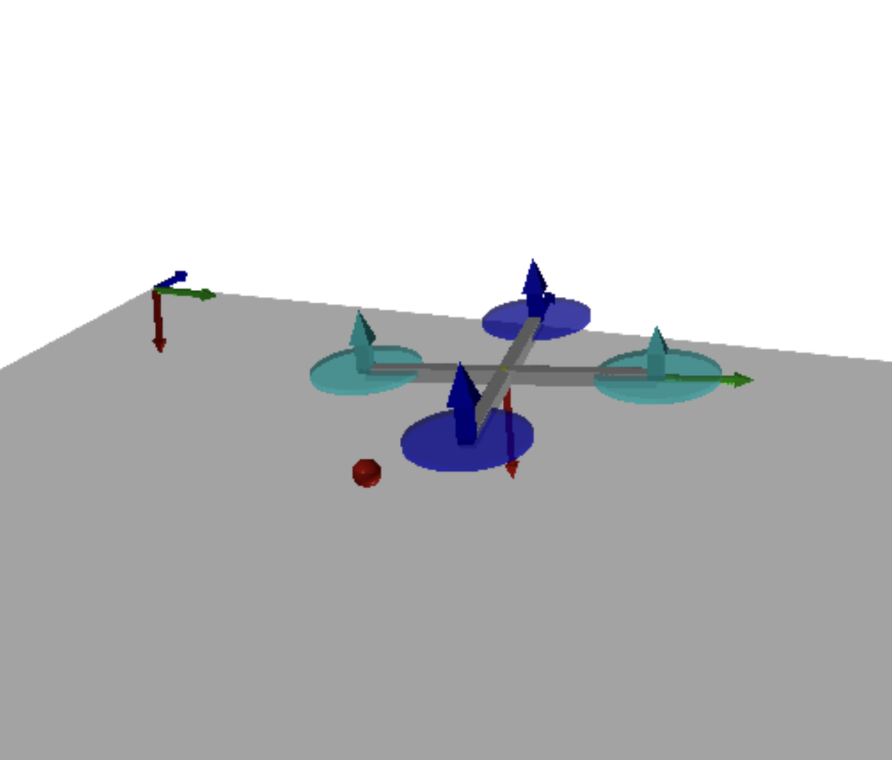
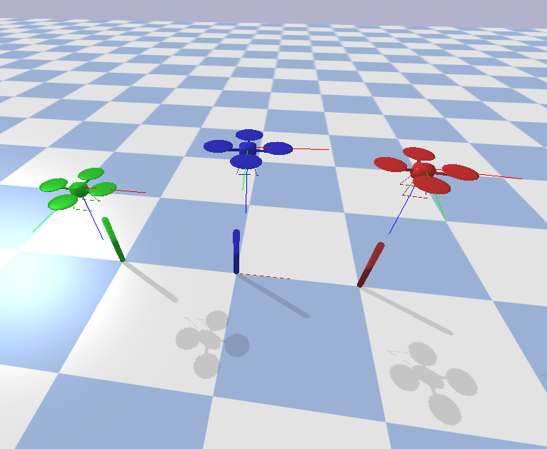
Figure 3: Simulation environments: (left) simplified custom environment for training. (right) real-time physics environment, gym-pybullet-drones [20], for sim-to-sim verification for each scheme of SARL (green), DTDE (blue), and CTDE (red).

Our proposed frameworks can be trained with any MARL algorithm, and in this study, we selected TD3 and MATD3 which are model-free, off-policy, actor-critic algorithms.

Network Structures. In our experiment, the actor networks are multilayer perceptron (MLP) networks with two hidden layers of 16 nodes each, using the rectified linear unit (ReLU) activation function. The actor networks map the states $s_{t}$ or observations $o_{t}$ to actions $a_{t}$ at time $t$. The hyperbolic tangent (tanh) activation function is used in the output layer of the actor network to ensure a proper range of control signals between $[-1,1]$. The critic networks take both states and actions as inputs and estimate the action-value function $Q^{\pi}(s_{t},a_{t})$ as outputs. The critic networks are also designed as MLP networks with two hidden layers of 512 nodes each, using the ReLU activation function.

Hyperparameters. The reward coefficients $k_{x}$ and $k_{b_{1}}$ in Section IV are set to 7.0 and 2.0, respectively, to minimize tracking errors in position and heading. To eliminate steady-state error, $k_{I_{x}}$ and $k_{I_{b_{1}}}$ are chosen as 0.04 and 0.06, with $\alpha=0.01$ in (24). Also, the penalizing terms are set to $k_{v}=k_{\Omega}=k_{\omega_{12}}=0.25$, $k_{b_{3}}=3.5$, and $k_{\Omega_{3}}=0.2$ to achieve smooth and stable control. We found that excessively large penalties can prevent the quadrotor from moving toward its target by causing it to focus too much on stabilization. The selected hyperparameters are summarized in Table II.

TABLE II: Hyperparameters.

Parameter	Value
Optimizer	AdamW
Learning rate	$1\times 10^{-4}\rightarrow 1\times 10^{-6}$
Discount factor, $\gamma$	0.99
Replay buffer size	$10^{6}$
Batch size	256
Maximum global norm	100
Exploration noise	0.3 $\rightarrow$ 0.05
Target policy noise	0.2
Policy noise clip	0.5
Target update interval	3
Target smoothing coefficient	0.005

Training Method. We trained our models for 3.5 million timesteps on a GPU workstation powered by NVIDIA A100-PCIE-40GB. The learning rate is scheduled with SGDR [21] to avoid over-fitting, and the exploration noise is decayed. To encourage exploration, we randomly select all states of each episode from predefined distributions, e.g., randomly placing the quadrotor in $3\mathrm{m}\times 3\mathrm{m}\times 3\mathrm{m}$ space. During training and evaluation, both state and action are normalized to $[-1,1]$ to speed up the training process while improving stability. Similarly, we normalized each step’s reward to $[0,1]$ to ensure convergence. Note that agents in this study were trained without pre-training or any auxiliary aid techniques such as PID controllers.

Domain Randomization. RL agents trained in simulators often suffer from performance degradation when deployed to another simulation environment or the real world. This is due to the discrepancy between the training environment and the testing environment caused by parametric uncertainties or unmodeled dynamics. Domain randomization is one of the promising methods to bridge the resulting sim-to-sim gap or sim-to-real gap, where the properties of the training environment are randomized to allow the agents to adapt and generalize under varying conditions [10]. In this paper, at the start of each training episode, the physical parameters of the simulator are sampled uniformly from the $\pm 5\%$ range around the nominal values listed in Table I.

V-B Benchmark Results

To benchmark the performance of each framework, we evaluated our trained policies at every 10,000 steps without exploration noise. The resulting learning curves showing the average return over 5 random seeds are presented in Figure 4. These are smoothed by the exponential moving average with a smoothing weight of 0.8, where the solid line and the shaded area represent the average and its 2$\sigma$ bounds over random seeds, respectively.

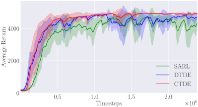
Figure 4: Learning curves for each framework over timesteps. The solid lines and shaded areas represent the average and standard deviation of performance, respectively.

First, the proposed MARL frameworks, namely DTDE and CTDE, exhibit faster and more robust convergence compared with the traditional single-agent framework, SARL. It illustrates that the proposed MARL framework with the decoupled dynamics improves the efficiency in learning by specializing each agent to its own task.

Next, we compare the performance of DTDE and CTDE. The learning curves show that CTDE is more stable over training than DTDE. In the first part of the training, both agents perform similarly, achieving a higher reward relatively faster than SARL. However, agents trained with CTDE exhibit more consistent training afterward, and the advantage of CTDE becomes more apparent as the number of time steps increases. We also found that in DTDE settings, the second agent for yawing control tends to generate an aggressive torque $M_{3}$, being too focused on its own goal.

We hypothesize that the primary cause of failure is non-stationarity. In single-agent settings, the agent’s decisions exclusively affect the environment, and state transitions can be clearly attributed to the agent, while external factors are considered part of the system dynamics. However, in multi-agent scenarios, agents update their policies simultaneously during learning, leading to non-stationarity and the violation of the Markov property [22]. This presents a challenge known as the moving target problem in MARL, where agents face a dynamically changing environment. In DTDE, two agents do not share information, which can make it difficult for them to coordinate their actions and achieve higher rewards. In CTDE, on the other hand, two agents share information about their states and actions through the centralized critic networks, which allows them to better coordinate their decisions.

V-C Flight Trajectory with Large Yaw Angle

Next, we present the flight trajectories controlled by each framework. Figure 5 shows the flight performance of trained agents with an initial yaw error of 140 degrees. The position errors $e_{x}$ and attitude errors $e_{R}$ of the proposed method, DTDE and CTDE, are respectively denoted by blue and red lines. For comparison, the results of the single-agent method, SARL, are represented by green lines. While the agent trained with SARL failed to stabilize at the goal position and exhibited large overshoots and oscillations, the DTDE and CTDE agents achieved smaller errors by separating yaw control from roll and pitch control, However, DTDE showed significantly larger oscillations in $e_{x}$ and $e_{R}$ compared to CTDE. Therefore, our results demonstrate that centralized training is superior to decentralized training in terms of both flight performance as well as training stability.

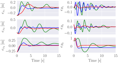
Figure 5: Flight performance of SARL (green), DTDE (blue), and CTDE (red) in the training environment. ($1^{\mathrm{st}}$ column) position error, $e_{x}=x-x_{d}\in\mathbb{R}^{3}$, ($2^{\mathrm{nd}}$ column) attitude error, $e_{R}=\frac{1}{2}(R_{d}^{T}R-R^{T}R_{d})^{\vee}\in\mathbb{R}^{3}$.

V-D Sim-to-Sim Transfer

To perform sim-to-sim transfer and validation, we export the trained agents into a more realistic physical environment developed by gym-pybullet-drones [20]. We evaluated our models under the same initial conditions as in Figure 5 for comparison, and the flight results are shown in Figure 6. Table III summarizes the average errors $e_{\mathrm{avg}}$ and steady-state errors $e_{\mathrm{ss}}$ in position and attitude for each framework in both training and evaluation environments.

Notably, the quadrotor trained with SARL crashed in the transferred environment, and DTDE exhibits oscillation similar to the above. In comparison, CTDE maintained a stable flight and achieved satisfactory flight performance in a realistic setting without additional training in the target domain, suggesting that it is generalizable to new environments.

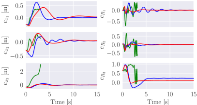
Figure 6: Sim-to-sim verification of SARL (green), DTDE (blue), and CTDE (red) in the physics environment. ($1^{\mathrm{st}}$ column) position error, $e_{x}=x-x_{d}\in\mathbb{R}^{3}$, ($2^{\mathrm{nd}}$ column) attitude error, $e_{R}=\frac{1}{2}(R_{d}^{T}R-R^{T}R_{d})^{\vee}\in\mathbb{R}^{3}$.

TABLE III: Position and attitude errors of each framework in training and evaluation environments. Average and steady-state error of position, $e_{x_{\mathrm{avg}}}$ and $e_{x_{\mathrm{ss}}}$, are in centimeters.

Fig. 5	SARL	DTDE	CTDE
$e_{x_{\mathrm{avg}}}$	(7.47, 15.2, 12.8)	(4.35, 3.50, 3.89)	(6.17, 7.13, 1.78)
$e_{x_{\mathrm{ss}}}$	(0.90, -13.7, 7.6)	(-2.57, 0.22, 1.44)	(0.59, -4.01, 0.15)
$e_{R_{\mathrm{avg}}}$	(0.03, 0.02, 0.29)	(0.03, 0.01, 0.23)	(0.01, 0.0, 0.14)
$e_{R_{\mathrm{ss}}}$	(0.01, 0.0, -0.03)	(0.0, 0.0, -0.19)	(0.0, 0.0, 0.11)
Fig. 6	SARL	DTDE	CTDE
$e_{x_{\mathrm{avg}}}$		(9.81, 10.1, 8.11)	(12.4, 8.88, 5.91)
$e_{x_{\mathrm{ss}}}$	Crashed	(-0.68, 3.64, -0.08)	(1.88, 4.30, -1.08)
$e_{R_{\mathrm{avg}}}$		(0.05, 0.03, 0.26)	(0.02, 0.02, 0.15)
$e_{R_{\mathrm{ss}}}$		(0.0, 0.0, 0.23)	(0.0, 0.0, 0.11)

VI Conclusion

In this paper, we present a multi-agent reinforcement learning framework for quadrotor low-level control, by decomposing the quadrotor dynamics into the translational part and the yawing part with distinct characteristics. Moreover, we introduce regularization terms to mitigate steady-state errors and prevent aggressive control inputs, promoting efficient control. We demonstrate that our MARL frameworks outperform traditional single-agent counterparts through numerical simulations and sim-to-sim verification, significantly reducing training time while maintaining reasonable control performance.

While simulations provide a valuable proving ground, we plan to validate our framework through actual flight experiments, known as sim-to-real transfer, along with the exploration of domain randomization or adaptation techniques to close the reality gap in multi-agent settings. This framework holds great promise for enhancing the training efficiency of RL-based quadrotor controllers.

References

- [1] J. Hwangbo, I. Sa, R. Siegwart, and M. Hutter, “Control of a quadrotor with reinforcement learning,” IEEE Robotics and Automation Letters, vol. 2, no. 4, pp. 2096–2103, 2017.
- [2] Y. Song, M. Steinweg, E. Kaufmann, and D. Scaramuzza, “Autonomous drone racing with deep reinforcement learning,” in International Conference on Intelligent Robots and Systems, 2021, pp. 1205–1212.
- [3] S. Belkhale, R. Li, G. Kahn, R. McAllister, R. Calandra, and S. Levine, “Model-based meta-reinforcement learning for flight with suspended payloads,” IEEE Robotics and Automation Letters, vol. 6, no. 2, pp. 1471–1478, 2021.
- [4] T. Lee, M. Leok, and N. H. McClamroch, “Geometric tracking control of a quadrotor UAV on SE(3),” in IEEE conference on decision and control, 2010, pp. 5420–5425.
- [5] K. Gamagedara, M. Bisheban, E. Kaufman, and T. Lee, “Geometric controls of a quadrotor UAV with decoupled yaw control,” in 2019 American Control Conference (ACC). IEEE, 2019, pp. 3285–3290.
- [6] J. Ackermann, V. Gabler, T. Osa, and M. Sugiyama, “Reducing overestimation bias in multi-agent domains using double centralized critics,” arXiv preprint arXiv:1910.01465, 2019.
- [7] S. Fujimoto, H. Hoof, and D. Meger, “Addressing function approximation error in actor-critic methods,” in International conference on machine learning. PMLR, 2018, pp. 1587–1596.
- [8] C.-H. Pi, K.-C. Hu, S. Cheng, and I.-C. Wu, “Low-level autonomous control and tracking of quadrotor using reinforcement learning,” Control Engineering Practice, vol. 95, p. 104222, 2020.
- [9] C.-H. Pi, Y.-W. Dai, K.-C. Hu, and S. Cheng, “General purpose low-level reinforcement learning control for multi-axis rotor aerial vehicles,” Sensors, vol. 21, no. 13, p. 4560, 2021.
- [10] A. Molchanov, T. Chen, W. Hönig, J. A. Preiss, N. Ayanian, and G. S. Sukhatme, “Sim-to-(multi)-real: Transfer of low-level robust control policies to multiple quadrotors,” in International Conference on Intelligent Robots and Systems, 2019, pp. 59–66.
- [11] B. Yu and T. Lee, “Equivariant reinforcement learning for quadrotor UAV,” in 2023 American Control Conference (ACC). IEEE, 2023, pp. 2842–2847.
- [12] B. Li, S. Li, C. Wang, R. Fan, J. Shao, and G. Xie, “Distributed circle formation control for quadrotors based on multi-agent deep reinforcement learning,” in 2021 China Automation Congress (CAC). IEEE, 2021, pp. 4750–4755.
- [13] R. Zhang, Q. Zong, X. Zhang, L. Dou, and B. Tian, “Game of drones: Multi-UAV pursuit-evasion game with online motion planning by deep reinforcement learning,” IEEE Transactions on Neural Networks and Learning Systems, 2022.
- [14] R. Ourari, K. Cui, A. Elshamanhory, and H. Koeppl, “Nearest-neighbor-based collision avoidance for quadrotors via reinforcement learning,” in 2022 International Conference on Robotics and Automation (ICRA). IEEE, 2022, pp. 293–300.
- [15] H. Han, J. Cheng, Z. Xi, and B. Yao, “Cascade flight control of quadrotors based on deep reinforcement learning,” IEEE Robotics and Automation Letters, vol. 7, no. 4, pp. 11 134–11 141, 2022.
- [16] K. Gamagedara and T. Lee, “Geometric adaptive controls of a quadrotor unmanned aerial vehicle with decoupled attitude dynamics,” Journal of Dynamic Systems, Measurement, and Control, vol. 144, no. 3, p. 031002, 2022.
- [17] R. Lowe, Y. I. Wu, A. Tamar, J. Harb, O. Pieter Abbeel, and I. Mordatch, “Multi-agent actor-critic for mixed cooperative-competitive environments,” Advances in neural information processing systems, vol. 30, 2017.
- [18] S. Mysore, B. Mabsout, R. Mancuso, and K. Saenko, “Regularizing action policies for smooth control with reinforcement learning,” in 2021 IEEE International Conference on Robotics and Automation (ICRA). IEEE, 2021, pp. 1810–1816.
- [19] G. C. Lopes, M. Ferreira, A. da Silva Simoes, and E. L. Colombini, “Intelligent control of a quadrotor with proximal policy optimization reinforcement learning,” in 2018 Latin American Robotic Symposium, 2018 Brazilian Symposium on Robotics (SBR) and 2018 Workshop on Robotics in Education (WRE), 2018, pp. 503–508.
- [20] J. Panerati, H. Zheng, S. Zhou, J. Xu, A. Prorok, and A. P. Schoellig, “Learning to fly—a Gym environment with PyBullet physics for reinforcement learning of multi-agent quadcopter control,” in 2021 IEEE/RSJ International Conference on Intelligent Robots and Systems (IROS). IEEE, 2021, pp. 7512–7519.
- [21] I. Loshchilov and F. Hutter, “SGDR: Stochastic gradient descent with warm restarts,” arXiv preprint arXiv:1608.03983, 2016.
- [22] L. Busoniu, R. Babuska, and B. De Schutter, “A comprehensive survey of multiagent reinforcement learning,” IEEE Transactions on Systems, Man, and Cybernetics, Part C (Applications and Reviews), vol. 38, no. 2, pp. 156–172, 2008.