A Compiler from Array Programs to Vectorized Homomorphic Encryption

Abstract.

Homomorphic encryption (HE) is a practical approach to secure computation over encrypted data. However, writing programs with efficient HE implementations remains the purview of experts. A difficult barrier for programmability is that efficiency requires operations to be vectorized in inobvious ways, forcing efficient HE programs to manipulate ciphertexts with complex data layouts and to interleave computations with data movement primitives.

We present Viaduct-HE, a compiler generates efficient vectorized HE programs. Viaduct-HE can generate both the operations and complex data layouts required for efficient HE programs. The source language of Viaduct-HE is array-oriented, enabling the compiler to have a simple representation of possible vectorization schedules. With such a representation, the compiler searches the space of possible vectorization schedules and finds those with efficient data layouts. After finding a vectorization schedule, Viaduct-HE further optimizes HE programs through term rewriting. The compiler has extension points to customize the exploration of vectorization schedules, to customize the cost model for HE programs, and to add back ends for new HE libraries.

Our evaluation of the prototype Viaduct-HE compiler shows that it produces efficient vectorized HE programs with sophisticated data layouts and optimizations comparable to those designed by experts.

1. Introduction

Homomorphic encryption (HE), which allows computations to be performed on encrypted data, has recently emerged as a viable way for securely offload computation. Efficient libraries (Chen et al., 2017) and hardware acceleration (Reagen et al., 2021; Riazi et al., 2020) have improved performance to be acceptable for practical use in a diverse range of applications such as the Password Monitor in the Microsoft Edge web browser (Lauter et al., 2021), privacy-preserving machine learning (Gilad-Bachrach et al., 2016), privacy-preserving genomics (Kim et al., 2021), and private information retrieval (Menon and Wu, 2022).

Writing programs to be executed under HE, however, remains a forbidding challenge (Viand et al., 2021). In particular, modern HE schemes support data encodings that allow for single-instruction, multiple data (SIMD) computation with very long vector widths but limited data movement capability. SIMD parallelism allows developers to recoup the performance loss of executing programs in HE, but taking advantage of this capability requires significant expertise: efficient vectorized HE programs requires carefully laying out data in ciphertexts and interleaving data movement operations with computations. There is a large literature on efficient, expert-written vectorized HE implementations (Juvekar et al., 2018; Gilad-Bachrach et al., 2016; Brutzkus et al., 2019; Aharoni et al., 2023; Kim et al., 2023).

Prior work has developed compilers to ease the programmability burden of HE, but most work has targeted specific applications (Dathathri et al., 2019; van Elsloo et al., 2019; Boemer et al., 2019b, a; Aharoni et al., 2023; Malik et al., 2021), or focuses on challenges other than vectorization (Dathathri et al., 2020; Lee et al., 2022; Crockett et al., 2018; Archer et al., 2019). Some HE compilers do attempt to generate vectorized implementations for arbitrary programs, but either fix simple data layouts for all programs (Viand et al., 2022) or require users to provide at least some information about complex data layouts (Cowan et al., 2021; Malik et al., 2023).

We make the important observation that the complex, expert-written data layouts targeting specific applications in prior work are made possible by array-level reasoning. That is, given an array as input to an HE program, searching for an efficient layout amounts to asking such questions as “should this dimension of the array be vectorized in a single ciphertext, or be exploded along multiple ciphertexts?” This kind of reasoning is not reflected in the prior work on HE compilers, but as we show, it enables vectorized HE implementations with expert-level efficiency.

With this in mind, we reframe the problem of compiling efficient vectorized HE programs as two separate problems. First, a program must be “tensorized” and expressed as an array program. In many cases, this step is actually unnecessary, since the program can already be naturally expressed as operations over arrays. This is true for many HE applications, such as secure neural network inference. Once expressed as a computation over arrays, the space of possible vectorization schedules for the program can be given a simple, well-defined representation. This makes the “last-mile” vectorization of array programs much more tractable than the vectorization of arbitrary imperative programs.

This “tensorize-then-vectorize” approach is arguably already present in the literature. For example, Malik et al. (2021) developed an efficient vectorized HE implementation for evaluating decision forests by expressing the evaluation algorithm as a sequence of element-wise array operations and matrix–vector multiplication, and then using an existing kernel (Halevi and Shoup, 2014) to implement matrix–vector multiplication efficiently.

In this paper, we aim to tackle the challenge of generating vectorized HE implementations for array programs. To this end, we propose Viaduct-HE, a vectorizing HE compiler for an array-oriented source language. Viaduct-HE simultaneously generates the complex data layouts and operations required for efficient HE implementations. Unlike in prior work (Cowan et al., 2021; Malik et al., 2023), this process is completely automatic: the compiler needs no user hints to generate complex layouts. The compiler leverages the high-level array structure of source programs to give a simple representation for possible vectorization schedules, allowing it to efficiently explore the space of schedules and find efficient data layouts. Once a schedule has been found, the compiler can further optimize the program by translating it to an intermediate representation amenable to term rewriting.

Viaduct-HE is designed to be extensible: after optimization, the compiler translates circuits into a loop nest representation designed for easy translation into operations exposed by HE libraries, allowing for the straightforward development of back ends that target new HE implementations. The compiler also has well-defined extension points for customizing the exploration of vectorization schedules and for estimating the cost of HE programs.

We make the following contributions:

• A high-level array-oriented source language that can express a wide variety of programs that target vectorized homomorphic encryption.

• New abstractions to represent vectorization schedules and to control the exploration of the schedule search space for array-oriented HE programs, facilitating automated search for efficient data layouts.

• Intermediate representations that enable optimization through term rewriting and easy development of back ends for new HE libraries.

• A prototype implementation of the Viaduct-HE compiler and an evaluation that shows that the prototype automatically generates efficient vectorized HE programs with sophisticated layouts comparable to those developed by experts.

2. Background on Homomorphic Encryption

Homomorphic encryption schemes allow for operations on ciphertexts, enabling computations to be securely offloaded to third parties without leaking information about the encrypted data. Such schemes are homomorphic in that ciphertext operations correspond to plaintext operations: given encryption and decryption functions Enc and Dec, for a function $f$ there exists a function $f^{\prime}$ such that $f(x)=\textbf{Dec}(f^{\prime}(\textbf{Enc}(x)))$.

In a typical setting involving homomorphic encryption, a client encrypts their data with a private key and sends the ciphertext to a third-party server. The server performs operations over the ciphertext, and then sends the resulting ciphertext back to the client. The client can then decrypt the ciphertext to get the actual result of the computation.

We target modern lattice-based homomorphic encryption schemes such as BFV (Fan and Vercauteren, 2012), BGV (Brakerski et al., 2014), and CKKS (Cheon et al., 2017). In these schemes, ciphertexts can encode many data elements at once. Thus we can treat ciphertexts as vectors of data elements. Homomorphic computations are expressed as addition and multiplication operations over ciphertexts. Addition and multiplication execute element-wise over encrypted data elements, allowing for SIMD processing: given ciphertexts $x=\textbf{Enc}([x_{1},x_{2},\ldots,x_{n}])$ and $y=\textbf{Enc}([y_{1},y_{2},\ldots,y_{n}])$, homomorphic addition $\oplus$ and multiplication $\otimes$ operate such that

$$\textbf{Dec}(x\oplus y)=[x_{1}+y_{1},x_{2}+y_{2},\ldots,x_{n}+y_{n}]\;\;\;\;\;\;\;\;\textbf{Dec}(x\otimes y)=[x_{1}\times y_{1},x_{2}\times y_{2},\ldots,x_{n}\times y_{n}].$$

There are analogous addition and multiplication operations between ciphertexts and plaintexts, which also have a vector structure. This allows computation over ciphertexts using data known to the server. For example, it is common to multiply a ciphertext with a plaintext mask consisting of 1s and 0s to zero out certain slots of the ciphertext.

Along with addition and multiplication, rotation facilitates data movement, cyclically shifting the slots of data elements by a specified amount. For example,

$$\textbf{Dec}(\textup{rot}(-1,x))=[x_{2},x_{3},\ldots,x_{n},x_{1}]\;\;\;\;\;\;\;\;\textbf{Dec}(\textup{rot}(2,x))=[x_{n-1},x_{n},x_{1},\ldots,x_{n-2}].$$

2.1. Programmability Challenges

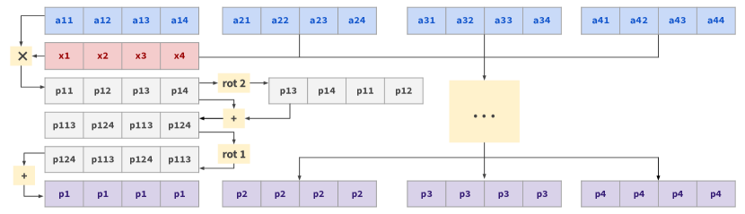
(a) Row-wise layout.

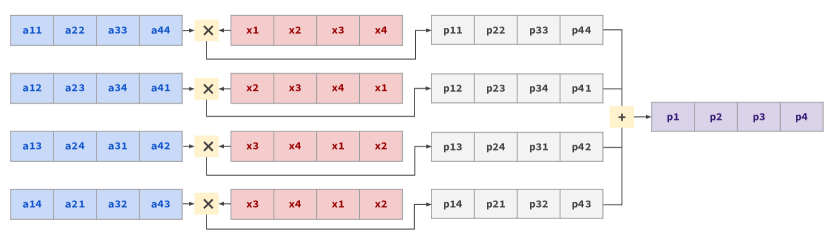
(b) Diagonal layout.

Figure 1. Different layouts for matrix–vector multiplication. Vectors from matrix a are in blue; vectors from vector v are in red; the output vectors are in violet.

While vectorized homomorphic encryption presents a viable approach to secure computation, there are many challenges to developing programs that use it. Such challenges include the lack of support for data-dependent control flow that forces programs to be written in “circuit” form; the selection of cryptographic parameters that are highly sensitive to the computations being executed; the management of ciphertext noise; and the interleaving of low-level “ciphertext maintenance” operations with computations (Viand et al., 2021).

Here we focus on the challenge of writing vectorized programs that use the SIMD capability of HE schemes. Efficiently vectorized HE programs are very different from programs in other regimes supporting SIMD. We now highlight some of the novelties of vectorizing in the HE regime.

Very long vector widths

Vector widths in HE ciphertexts are large powers of two—on the order of thousands when the scheme’s parameters are set to appropriate security levels (Albrecht et al., 2018). To take advantage of such a large number of slots, often times HE programs are structured in counterintuitive ways. For example, the convolution kernel in Gazelle (Juvekar et al., 2018) applies a filter to all output pixels simultaneously. COPSE (Malik et al., 2021) evaluates decision forests by evaluating all branches at once and then applies masking to determine the right classification label for an input.

Limited data movement

Although ciphertexts can be treated as vectors, they have a very limited interface. In particular, one cannot index into a ciphertext to retrieve individual data elements. All operations are SIMD and compute on entire ciphertexts at once. Thus expressing computation that operates on individual data elements as ciphertext operations can be challenging. One might consider naive approaches to avoid such difficulties; for example, ciphertexts can be treated as single data elements by only using their first slot. Failure to restructure programs to take advantage of the SIMD capability of HE, however, exacts a steep performance hit: in many cases, orders of magnitude in slowdown (Viand et al., 2022).

So in practice, data elements must be packed in ciphertexts to write efficient HE programs. However, packing creates new problems: if an operation requires data on different slots, ciphertexts must be rotated to align the operands. One is thus forced to interleave data movement and computation, but determining how to schedule these together efficiently can be difficult.

Because rotation operations provide limited data movement, the initial data layout in ciphertexts has a great impact on the efficiency of HE programs. One layout might aggressively pack data to minimize the number of ciphertexts the client needs to send and also minimize the computations the server needs to perform, but might require too many rotations; another layout might not aggressively pack data into ciphertexts to avoid the necessity of data movement operations, but might force greater client communication and the server to perform more computations.

Example: Matrix–vector multiplication

To illustrate the challenges of developing vectorized HE programs, consider the two implementations of matrix–vector multiplication shown in Figure 1. Here a matrix a is multiplied with a vector x; the vectors containing data elements from a are in blue, while the vectors containing data elements from x are in red; the output vectors of the multiplication are in purple.

Figure 1(a) shows a row-wise layout for the program, where the each of the blue vectors represents a row from a. A single red vector contains the vector x. The figure shows the computation of a dot product for one row of a and x; First, the vectors are multiplied, and then the product vector is rotated and added with itself multiple times to compute the sum. This pattern, which we call rotate-and-reduce, is common in the literature (Cowan et al., 2021; Viand et al., 2022; Kim et al., 2023) and it exploits it allows for computing reductions in a logarithmic number of operations relative to the number of elements. Here 4 elements can be summed with 2 rotations and 2 additions. The row-wise layout results in the dot product outputs to be spread out in 4 ciphertexts, which can preclude further computation (they cannot be used as a packed vector in another matrix–vector multiplication, say) and induce a lot of communication if the server sends these outputs to the client.

Figure 1(b) shows the “generalized diagonal” layout from Halevi and Shoup (2014). Here the vectors contain diagonals from array a: the first vector contains the main diagonal; the second vector contains a diagonal shifted to the right and wrapped around; and so on. These vectors are then multiplied with the vector containing x, but rotated an appropriate number of slots. The layout of the product vectors allow the sum to be computed simply by adding the vectors together, as the product elements for different rows are packed in the same vector but elements for the same row are “exploded” along multiple vectors.

In total, the diagonal layout requires only 3 rotations and 3 additions, compared to the 8 additions and 8 rotations required by the row-wise layout. Additionally, the outputs are packed in a single vector, which can be convenient for further computations (it can be used as input to another matrix–vector multiplication) or for returning results to the client with minimal communication.

3. Compiler Overview

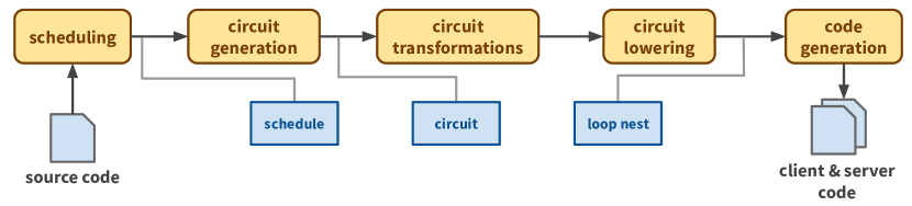
Figure 2. Viaduct-HE compiler architecture.

⬇

input a: [4, 4] from server

input x: [4] from client

for j: 4 {

sum(for i: 4 {

(a[j][i] - x[i]) *

(a[j][i] - x[i])

})

}

(a) Source code.

⬇

let out =

sum_vec(i: 4,

(at - rot(i, xt)) *

(at - rot(i, xt)))

(b) Circuit representation.

⬇

at = PlaintextArray([4])

tmp0 = Vec(a,Roll(1,0),[0,0],

[(2,0,0,{(0,1)}])

at[0] = encode(tmp0)

...

xt = CiphertextArray([4])

xt[0] = Vec(x,Id,[0],[(4,0,0,{(0,1)})])

...

out = CiphertextArray([])

for i in range(4) {

inst1 = rot(C,i,xt[i])

inst2 = sub(CP,inst1,at[i])

inst3 = mul(C,inst2,inst2)

out = add(C,out,inst3)

}

(c) Loop-nest representation.

Figure 4. Compilation of the distance program.

Figure 2 shows the architecture of the Viaduct-HE compiler. It takes as input an array program and generates both code run by the client, which sends inputs and receives program results, and by the server, which performs the computations that implement the source program. The compiler has well-defined extension points to control different aspects of the compilation process. To describe this process in detail, we consider the compilation of a program that computes the distance of a client-provided point (x) against a list of test points known to the server (a).

3.1. Source Language

Figure 4(a) shows the source code for the distance program. It specifies that a is a 2D array provided as input by the server, with an extent of 4 on both dimensions; similarly, x is a 1D array provided as input by the client, with an extent of 4. Thus a is assumed to be known to the server and thus is in plaintext, while x is in ciphertext since it comes from the client. The two for nodes each introduce a new dimension to the output array; they also introduce the index variables i and j, which are used to index into the input arrays a and x. The dimension introduced by the inner for node is reduced with the sum operator, so the output array has one dimension. Conceptually, the program computes the distance of x from the rows of a, each of which represents a point. An equivalent implementation in a traditional imperative language would look like the following program on the left.

⬇

a = Array[4][4];

x = Array[4];

out = Array[4]

for (j = 0; j < 4; j++) {

acc = 0;

for (i = 0 ; i < 4; i++) {

acc += (a[j][i] - x[i]) *

(a[j][i] - x[i]);

}

out[j] = acc;

}

Figure 5 defines the abstract syntax for the source language. Programs consist of a sequence of inputs and let-bound expressions followed by an output expression whose result the server sends to the client. Expressions uniformly denote arrays; scalars are considered zero-dimensional arrays. The expression input $a:sh$ from $pt$ in $e$ denotes an array with shape $sh$ received as input from $pt$, which is either the client or the server. Input arrays from the client are treated as ciphertexts, while input arrays from the server are treated as plaintexts. Operation expression $e_{1}\odot e_{2}$ denotes an element-wise operation over equal-dimension arrays denoted by $e_{1}$ and $e_{2}$, while reduction expression $\textbf{reduce}_{\odot,n}(e)$ reduces the $n$-th dimension of the array denoted by $e$ using $\odot$.

The expression for $i:n$ $\{e\}$ adds a new outermost dimension with extent $n$ to the array denoted by $e$, while $e[in]$—also referred throughout as an indexing site—indexes the outermost dimension of an array. Only array variables, introduced by inputs or let-bindings, can be indexed. The compiler also imposes some restrictions on indexing expressions. Particularly, index variables cannot be multiplied together (e.g. a[i*j]), as compiler analyses assume that the dimensions of indexed arrays are traversed with constant stride.

$$\begin{array}[]{llcl}\lx@intercol\textrm{Integer }z\in\mathbb{Z}\hfill\textrm{Natural }n\in\mathbb{N}\hfill\textrm{Index variable }i,j,k\hfill\textrm{Array variable }a,b,c\hfil\lx@intercol\\[4.30554pt] \textrm{Shape}&sh&::=&[n_{1},\ldots,n_{d}]\\ \textrm{Party}&pt&::=&\textbf{client}\,\mid\,\textbf{server}\\ \textrm{Operator}&\odot&::=&+\,\mid\,-\,\mid\,\times\\ \textrm{Index}&in&::=&i\,\mid\,z\,\mid\,in\odot in\\ \textrm{Expression}&e&::=&z\,\mid\,ie\,\mid\,e\odot e\,\mid\,\textbf{reduce}_{\odot,n}(e)\,\mid\,\textbf{for $i:n$ $\{e\}$}\\ \textrm{Index Expression}&ie&::=&a\,\mid\,ie[in]\\ \textrm{Statement}&s&::=&\textbf{let $a=e$ in $s$}\,\mid\,\textbf{input $a:sh$ from $pt$ in $s$}\,\mid\,e\end{array}$$

Figure 5. Abstract syntax for the source language.

3.2. Scheduling

The source program is an abstract representation of computation over arrays; it represents the algorithm—the what—of an HE program. The vectorization schedule—how data will be represented by ciphertext and plaintext and how computations will be performed by HE operations—is left unspecified by the source program. Because its source language is array-oriented, the vectorization schedules for Viaduct-HE programs have a simple representation, allowing the compiler to manipulate such schedules and search for efficient ones during its scheduling stage. The compiler provides extension points to control both how the search space of schedules is explored and how the cost of schedules are assessed.

Like matrix multiplication, the distance program can be given a row-wise layout and a diagonal layout. The diagonal layout similarly requires less rotation and addition operations. The scheduling stage of the compiler can search for these schedules and assess their costs.

3.3. Circuit Representation

Once an efficient schedule has been found, the circuit generation stage of the compiler uses it to translate the source program into a circuit representation. The circuit representation represents information about the ciphertexts and plaintexts required in an HE program, as well as operations to be performed over these, at a very abstract level. The compiler has circuit transformation stages that leverage the algeraic properties of circuits to rewrite them into more efficient forms. Circuits are designed to facilitate optimization: a single circuit expression can represent many computations, so circuit rewrites can optimize many computations simultaneously.

Figure 4(b) shows the circuit representation for the distance program with the diagonal layout. The sum_vec operation represents a summation of 4 different vectors together into one vector. The 4 vectors each represent a the result of a squared difference computation between vector containing a generalized diagonal of array a (represented by the variable at) and a rotated vector containing array v (represented by the variable xt).

3.4. Loop-nest Representation

Circuits represent HE computations at a very high level. This makes the circuit representation amenable to optimization, but makes generation of target code difficult. After circuit programs have been optimized, the circuit lowering stage of the compiler translates circuit programs into a “loop-nest” representation. Loop-nest programs are imperative programs that are much closer in structure to target code. Once in the loop-nest representation, the code generation stage of the compiler generates target code using a back end for a specific HE library. The compiler can generate code for a different HE library just by swapping out the back end it uses. Back ends only need to translate loop-nest programs to target code, so adding support for new back ends is straightforward.

Figure 4(c) shows the loop-nest representation for the distance program. It contains code to explicitly fill in the variables at and xt with the vectors that will be used in computations. The summation is now represented as an explicit for loop that accumulates squared distance computations in an out variable.

4. Scheduling

The scheduling stage begins by first translating source programs into an intermediate representation that eliminates explicit indexing constructs. From there, the compiler generates an initial schedule and explores the search space of vectorization schedules.

4.1. Index-free Representation

The index-free representation is similar to the source language, except that for nodes are eliminated and indexing sites are replaced with pair $(is,at)$ of a unique identifier ($is$) and an array traversal ($at$) that summarizes the contents of the array denoted by the indexing site. Array traversals are arrays generated from indexing another array. The figure on the left shows the array traversals in the distance program. The traversal in red is from indexing array a; the traversal in blue is from indexing array x. Note that the dimension 0 is introduced by the for j node in the source program, while dimension 1 is introduced by the for i node. The traversal of array x repeats along dimension 0 because it is not indexed by j and thus does not change along that dimension.

Formally, array traversals have three components: the name of the indexed array; the integer offsets at which the traversal begins, defined by a list of integers with a length equal to the number of dimensions of the indexed array; and a list of traversal dimensions ($td$). We write $\textup{a}(z_{1},\ldots,z_{m})[td_{1},\ldots,td_{n}]$ to denote a $n$-dimensional traversal of an $m$-dimensional array. Array traversals can define positions that are out-of-bounds; for example, offsets can be negative even though all index positions in an array start at 0.

Each traversal dimension has an extent specifying its size and a set of content dimensions that specify how the dimensions traverses the indexed array. Content dimensions have a dimension index and a stride. For example, a traversal dimension $(4,\{0::2\})$ defines a traversal of an array along its zeroth dimension that spans 4 elements, where only every other element is traversed (i.e. the stride is 2). Traversal dimensions can have empty content dimension sets, which means that the array traversal does not vary along the dimension. We call these traversal dimensions empty.

For example, the index-free representation for the distance program is

⬇

sum(1, ((at1,at) - (xt1,xt)) * (((at2,at) - (xt2,xt))).

Variables at1 and at2 represent indexing sites with traversal at that indexes array a; variables xt1 and xt2 represent indexing sites with traversal xt that indexes array x. The array traversals denoted by these indexing sites is as follows:

$${{\leavevmode\lstinline{{\lst@@@set@language\lst@@@set@numbers\lst@@@set@frame\lst@@@set@rulecolor\small\tt{\@listingGroup{ltx_lst_identifier}{at}}}}}=\textup{a}(0,0)[(4,\{0::1\}),(4,\{1::1\})]\;\;\;\;\;\;\;\;\leavevmode\lstinline{{\lst@@@set@language\lst@@@set@numbers\lst@@@set@frame\lst@@@set@rulecolor\small\tt{\@listingGroup{ltx_lst_identifier}{xt}}}}}=\textup{x}(0)[(4,\{\}),(4,\{0::1\})].$$

The traversal at defines a 4x4 array where dimension 0 traverses dimension 0 of input array a with stride 1, and dimension 1 traverses dimension 1 of array a with stride 1. Meanwhile, the traversal xt also defines a 4x4 array, but its dimension 0 is empty and its dimension 1 traverses the only dimension of input array x with stride 1.

4.2. Representing Schedules

Schedules define a layout for the array traversals denoted by each indexing site in the index-free representation. The layout determines how an array traversal is represented as a set of vectors. One can think of layouts as a kind of traversal of array traversals themselves. Because of this, layouts are defined similarly to array traversals, except they do not specify offsets, as layouts always have offset 0 along every traversal dimension.

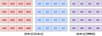
(a) Row-wise layout. Induces 5 input vectors, 4 output vectors, 8 additions, 8 rotations (2 adds and rotates per vector with rotate-and-reduce).

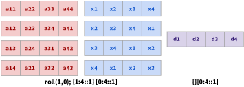
(b) “Diagonal” layout. Induces 5 input vectors, 1 output vector, 3 additions, 3 rotations.

Figure 6. Different schedules for the distance program.

Layouts are built from schedule dimensions which denote some part of an array traversal. We write the syntax $i:n::s$ for a schedule dimension with dimension index $i$, extent $n$, and stride $s$. For example, a schedule dimension $0:4::2$ defines a 4-element section of an array traversal along its zeroth dimension that contains only every other element (i.e. the stride is 2).

Concretely, layouts consist of the following: (1) a set of exploded dimensions; (2) a list of vectorized dimensions; and (3) a preprocessing operation. Exploded dimensions define parts of the array traversal that will be laid out in different vectors, while vectorized dimensions define parts that will be laid out in every vector. The ordering of vectorized dimensions defines their ordering on a vector: the beginning of the list defines the outermost vectorized dimensions, while the end defines the innermost vectorized dimensions. Preprocessing operations change the contents of the array traversal before being laid out into vectors, which allow for the representation of complex layouts. We write $p\{ed_{1},\ldots,ed_{m}\}[vd_{1},\ldots,vd_{n}]$ to denote a schedule with preprocessing $p$, $m$ exploded dimensions ($ed$) and $n$ vectorized dimensions ($vd$). When $p$ is the identity preprocessing operation, it is often omitted from the schedule.

Figure 6 shows two different schedules for the distance program. The vectors of at1 and at2 are in red, while the vectors of xt1 and xt2 are in blue. Their respective layouts are given below the vectors. Finally, the vectors of the distance program’s output is in purple, and the output layout is given below. Note that array traversals for at and xt must have the same layout since their arrays are multiplied together, and operands of element-wise operations must have the same layout.

Figure 6(a) represents a row-wise layout, where the entirety of dimension 1 of at and xt are vectorized while the entirety dimension 0 is exploded into multiple vectors. Thus traversal at is represented by 4 vectors, one for each of its rows; since traversal xt has 4 equal rows, it is represented by a single vector. Meanwhile, Figure 6(b) represents a “diagonal” layout; it is similar to a column-wise layout where each vector contains a column, but the roll preprocessing operation rotates the rows along the columns, where the rotation amount progressively increases. As discussed in Section 2, a similar diagonal layout was originally specified in Halevi and Shoup (2014) as an efficient implementation of matrix–vector multiplication, but here we see that the schedule abstraction can capture its essence, allowing the compiler to generalize and use it for other programs.

Note that exploded dimensions have a name associated with them; in the above syntax, the name for exploded dim $i$ is $d_{i}$. These names are used to uniquely identify vectors induced by the layout. During circuit generation, the names of exploded schedule dimensions will be used as variables that parameterize circuit expressions.

Preprocessing

A preprocessing operation in a layout transforms an array traversal before laying it out into vectors. Formally, a preprocessing operation is a permutation over elements of the array traversal. Thus we can think of preprocessing operations as functions from element positions to element positions. Given an $n$-dimensional array traversal $at$, applying preprocessing operation $p$ over $at$ defines a new traversal such that the element at position $x_{1},\ldots,x_{n}$ is the element at position $p(x_{1},\ldots,x_{n})$ of $at$. For example, the identity preprocessing operation is the trivial permutation that maps element positions to themselves: $\textup{id}=\lambda(x_{1},\ldots,x_{n}).(x_{1},\ldots,x_{n})$. Given that both dimensions $i$ and $j$ of an array traversal both have extent $n$, we can define the roll preprocessing operation as follows:

$$\textup{roll}(a,b)=\lambda(x_{1},\ldots,x_{a},\ldots,x_{b},\ldots,x_{n}).(x_{1},\ldots,x_{a}+x_{b}\;\%\;n,\ldots,x_{b},\ldots x_{n}).$$

Applying layouts

When applied to an array traversal, a layout generates a set of vectors that contain parts of the array indexed by the traversal. Formally, a vector contains four components: the name of the indexed array; a preprocessing operation; a list of integer offsets; and a list of traversal dimensions. As with preprocessing in a layout, a preprocessing operation in a vector transforms an array before its contents are laid out in the vector. We write $a.p(z_{1},\ldots,z_{m})[vtd_{1},\ldots,vtd_{n}]$ to denote a vector indexing an $m$-dimensional array $a$ with preprocessing $p$ and $n$ traversal dimensions ($vtd_{i}$). Again $p$ is usually elided when it is the identity preprocessing operation. Vector traversal dimensions are similar to array traversal dimensions, except they also track elements that are out-of-bounds. A vector can have out-of-bounds values either because its dimensions extend beyond the extents of the indexed array or the extents of the array traversal from which it is generated. We write $(n,obl,obr,\{cd_{1},\ldots,cd_{m}\})$ to denote a vector traversal dimension with extent $n$, $m$ content dimensions, a left out-of-bounds extent $obl$, and a right out-of-bounds extent $obr$. The left out-of-bounds and right out-of-bounds extents count the number of positions in a dimension that are out-of-bounds to the left and right of the in-bounds positions respectively. The compiler enforces the semantics that out-of-bounds values have value 0.

Given a layout with $n$ exploded dimensions each with extent $n_{i}$, applying the layout to an array traversal generates $\prod n_{i}$ vectors, one for each distinct combination of positions that can be defined along exploded dimensions. We call each such combination a coordinate. For example, when applied to array traversal at, the diagonal layout for the distance program generates 4 vectors, one for each distinct positions that the exploded dimension named $i$ can take:

$$\{i\mapsto 0\}\mapsto\textup{a}.\textup{roll}(1,0)(0,0)[(4,0,0,\{0::1\})] \{i\mapsto 1\}\mapsto\textup{a}.\textup{roll}(1,0)(0,1)[(4,0,0,\{0::1\})]$$

$$\{i\mapsto 2\}\mapsto\textup{a}.\textup{roll}(1,0)(0,2)[(4,0,0,\{0::1\})] \{i\mapsto 3\}\mapsto\textup{a}.\textup{roll}(1,0)(0,3)[(4,0,0,\{0::1\})].$$

This represents the same vectors for traversal at visually represented in Figure 6(b).

4.3. Searching for Schedules

To search for an efficient schedule for the program, the scheduling stage begins with an initial schedule where the layouts for all indexing sites contain only exploded dimensions. Thus in this schedule elements of arrays are placed in individual vectors. While very inefficient, the initial schedule can be defined for any program. To explore the search space of schedules, the scheduling stage uses a set of schedule transformers that take a schedule as input and returns a set of “nearby” schedules. To assess both the validity of a schedule visited during search, the compiler attempts to generate a circuit from the schedule. If a circuit is successfully generated, it is applied to a cost estimator function to determine the cost of the schedule.

The schedule transformers in the prototype implementation of the compiler include the following.

Vectorize dimension transformer

This transformer takes an exploded dimension from a layout and vectorizes it:

$$p\{\ldots,(d_{a})\;i_{a}:n_{a}::s_{a},\ldots\}[\ldots]\leadsto p\{\ldots\}[\ldots,i_{a}:n_{a}::s_{a}].$$

Importantly, this transformer only generates vectorized dimensions with extents that are powers of two; if the exploded dimension is not a power of two, the transformer will round up the vectorized dimension’s extent to the nearest one. The transformer imposes this limit on vectorized dimensions to simplify reasoning about correctness: vectors only wrap around correctly when their size divides the slot counts of ciphertexts and plaintexts without remainder, and these slot counts are always powers of two. This limitation also allows the circuit generation stage to uniformly use the rotate-and-reduce pattern.

Tiling transformer

This transformer takes an exploded dimension and tiles it into an outer dimension and an inner dimension. That is, given that extent $n_{a}$ can be split into $n$ tiles each of size $t$ (i.e., $e_{a}=tn$), it performs the following transformation:

$$p\{\ldots,(d_{a})\;i_{a}:n_{a}::s_{a},\ldots\}[\ldots]\leadsto p\{\ldots,(d_{a}^{\prime})\;i_{a}:t::s_{a},(d_{a}^{\prime\prime})\;i_{a}:n::s_{a}t,\ldots\}[\ldots]$$

where $d_{i}^{\prime}$ and $d_{i}^{\prime\prime}$ are fresh exploded dimension names.

Roll transformer

This transformer applies a roll preprocessing operation to a layout:

$$\textup{id}\{\ldots,(d_{a})\;i_{a}:n::s_{a},\ldots\}[i_{b}:n::s_{b},\ldots]\leadsto\textup{roll}(a,b)\{\ldots,(d_{a})\;i_{a}:n::s_{a},\ldots\}[i_{b}:n::s_{b},\ldots].$$

The transformer only applies when dimension $a$ is exploded, dimension $b$ is the outermost vectorized dimension and their extents match. Other conditions must hold to use a layout with roll preprocessing; we defer to the supplementary materials for more details.

Epochs

The search space for vectorization schedules is large. To control the amount of time that scheduling takes, the search is staggered into epochs. During an epoch, the configuration of schedule transformers is fixed such that only a subset of the search space is explored. When no more schedules can be visited, the epoch ends; a new epoch then begins with the schedule transformers updated to allow exploration of a bigger subset of the search space. The compiler runs a set number of epochs, after which it uses the most efficient schedule found to proceed to later stages of compilation.

The prototype implementation of the Viaduct-HE compiler uses epochs to control how schedule dimensions are split by the tiling transformer, which is the main cause of search space explosion. The tiling transformer gradually increases the number of schedule dimensions it splits as the number of scheduling epochs increase.

5. Circuit Generation

$$\begin{array}[]{llcl}\lx@intercol\textrm{Dimension variable }d\in\mathcal{D}\;\;\;\;\;\;\textrm{Array name }a\;\;\;\;\;\;\textrm{Vector }v\hfil\lx@intercol\\ \lx@intercol\textrm{Plaintext var }\varphi_{p}\;\;\;\;\;\;\textrm{Ciphertext var }\varphi_{c}\;\;\;\;\;\;\textrm{Offset var }\varphi_{o}\hfil\lx@intercol\textrm{Circuit value map }cm_{\tau}\in(\mathcal{D}\times\cdots\times\mathcal{D}\rightharpoonup\mathbb{N}\times\cdots\times\mathbb{N})\rightharpoonup\tau\end{array}$$

$$\begin{array}[]{llcl}\textrm{Offset}&oe&::=&d\,\mid\,z\,\mid\,oe\odot oe\,\mid\,\varphi_{o}\\ \textrm{Expression}&ce&::=&\varphi_{p}\,\mid\,\varphi_{c}\,\mid\,z\,\mid\,ce\odot ce\,\mid\,\textbf{rot}(oe,ce)\,\mid\,\textbf{reduce-vec}_{\odot}(d:n,ce)\\ \textrm{Statement}&cs&::=&\textbf{let $a:[d_{1}:n_{1},\ldots,d_{n}:n_{n}]=ce$ in $cs$}\,\mid\,\textbf{skip}\\ \textrm{Object}&co\in\mathcal{O}&::=&\textup{Const}(z)\,\mid\,\textup{Mask}(\overline{(n,n,n)})\,\mid\,\textup{Vec}(v)\\ \textrm{Registry}&cr&::=&\varphi_{o}\mapsto cm_{\mathbb{Z}},cr\,\mid\,\varphi_{p}\mapsto cm_{\mathcal{O}},cr\,\mid\,\varphi_{c}\mapsto cm_{\mathcal{O}},cr\,\mid\,\cdot\end{array}$$

Figure 7. Abstract syntax for circuit programs.

$$\begin{array}[]{llcl}\lx@intercol\textrm{Array Materializer }A\;\;\;\;\textrm{Layout }\ell\;\;\;\;\textrm{Index-free expression }fe\;\;\;\;\textrm{Index-free statement }fs\hfil\lx@intercol\\ \lx@intercol\textrm{Schedule dimension }sd\;\;\;\;\textrm{Exploded dimension }ed\hfil\lx@intercol\textrm{Output Vectorized Dimension }ovd::=i:n::s\,\mid\,\textup{R}(n)\,\mid\,\textup{RR}(n)\textrm{Output Layouts }o\ell::=\ast\,\mid\,p\{ed_{1},\ldots,ed_{m}\}[ovd_{1},\ldots,ovd_{n}]\textrm{Schedule }\Sigma::=\Sigma,is:\ell\,\mid\,\cdot\textrm{Input Context }\Gamma::=\Gamma,a:sh\,\mid\,\cdot\textrm{Expression Context }\Delta::=\Delta,a:(sh,o\ell)\,\mid\,\cdot\end{array}$$

$$\framebox{$A;\Sigma;\Gamma;\Delta\vdash fe\leadsto ce:(sh,o\ell)$}\penalty 50\hskip 20.00003pt plus 0.5fil minus 5.0pt\framebox{$A;\Sigma;\Gamma;\Delta\vdash fs\leadsto cs$}\penalty-10000\hskip 20.00003pt plus 0.5fil minus 5.0pt\raise 0.0pt\hbox{${\hbox{$\displaystyle\vbox{\hbox{\hskip 15.50229pt\vbox{\vbox{}\hbox{\hskip-15.50227pt\hbox{\hbox{$\displaystyle\displaystyle\ast<:sh$}}}}}}$}}\hbox{}$ }\penalty 50\hskip 20.00003pt plus 0.5fil minus 5.0pt\raise 0.0pt\hbox{${\hbox{$\displaystyle\vbox{\hbox{\hskip 14.7847pt\vbox{\vbox{}\hbox{\hskip-14.7847pt\hbox{\hbox{$\displaystyle\displaystyle\ast<:o\ell$}}}}}}$}}\hbox{}$ }\penalty 50\hskip 20.00003pt plus 0.5fil minus 5.0pt\raise 0.0pt\hbox{${\hbox{$\displaystyle\vbox{\hbox{\hskip 104.01547pt\vbox{\vbox{}\hbox{\hskip-104.01547pt\hbox{\hbox{$\displaystyle\displaystyle p\{\ldots\}[\textup{RR}(n),ovd_{2},\ldots,ovd_{n}]<:p\{\ldots\}[ovd_{2},\ldots,ovd_{n}]$}}}}}}$}}\hbox{}$ }\penalty-10000\hskip 20.00003pt plus 0.5fil minus 5.0pt\raise 0.0pt\hbox{${\vbox{\hbox{\hbox{\small\small{CGen-Literal}}}\hbox{$\displaystyle\displaystyle{\hbox{\hskip 1.38885pt\vbox{\hbox{\hskip-1.38885pt\hbox{\hbox{$\displaystyle\displaystyle\;$}}}\vbox{}}}\over\hbox{\hskip 50.43741pt\vbox{\vbox{}\hbox{\hskip-50.43741pt\hbox{\hbox{$\displaystyle\displaystyle A;\Sigma;\Gamma;\Delta\vdash z\leadsto z:(\ast,\ast)$}}}}}}$}}}\hbox{}$ }\penalty 50\hskip 20.00003pt plus 0.5fil minus 5.0pt\raise 0.0pt\hbox{${\vbox{\hbox{\hbox{\small\small{CGen-Op}}}\hbox{$\displaystyle\displaystyle{\hbox{\hskip 102.49944pt\vbox{\hbox{\hskip-102.49942pt\hbox{\hbox{$\displaystyle\displaystyle A;\Sigma;\Gamma;\Delta\vdash fe_{1}\leadsto ce_{1}:(sh,o\ell)$}\hskip 20.00003pt\hbox{\hskip-60.74037pt\hbox{\hbox{$\displaystyle\displaystyle A;\Sigma;\Gamma;\Delta\vdash fe_{2}\leadsto ce_{2}:(sh,o\ell)$}}}}}\vbox{\hbox{\hskip-60.74037pt\hbox{\hbox{$\displaystyle\displaystyle A;\Sigma;\Gamma;\Delta\vdash fe_{2}\leadsto ce_{2}:(sh,o\ell)$}}}\vbox{}}}}\over\hbox{\hskip 84.73538pt\vbox{\vbox{}\hbox{\hskip-84.73537pt\hbox{\hbox{$\displaystyle\displaystyle A;\Sigma;\Gamma;\Delta\vdash fe_{1}\odot fe_{2}\leadsto ce_{1}\odot ce_{2}:(sh,o\ell)$}}}}}}$}}}\hbox{}$ }\penalty 50\hskip 20.00003pt plus 0.5fil minus 5.0pt\raise 0.0pt\hbox{${\vbox{\hbox{\hbox{\small\small{CGen-Input-Index}}}\hbox{$\displaystyle\displaystyle{\hbox{\hskip 126.62056pt\vbox{\hbox{\hskip-126.62056pt\hbox{\hbox{$\displaystyle\displaystyle\Sigma(is)=\ell$}\hskip 20.00003pt\hbox{\hbox{$\displaystyle\displaystyle\Gamma(a)=sh_{a}$}\hskip 20.00003pt\hbox{\hskip-126.55237pt\hbox{\hbox{$\displaystyle\displaystyle a=\textsc{tr-array}(at)$}\hskip 20.00003pt\hbox{\hbox{$\displaystyle\displaystyle sh=\textsc{tr-shape}(at)$}\hskip 20.00003pt\hbox{\hskip-73.02007pt\hbox{\hbox{$\displaystyle\displaystyle\textsc{materialize-input}(A,sh_{a},at,\ell)\leadsto ce$}}}}}}}}}\vbox{\hbox{\hskip-126.55237pt\hbox{\hbox{$\displaystyle\displaystyle a=\textsc{tr-array}(at)$}\hskip 20.00003pt\hbox{\hbox{$\displaystyle\displaystyle sh=\textsc{tr-shape}(at)$}\hskip 20.00003pt\hbox{\hskip-73.02007pt\hbox{\hbox{$\displaystyle\displaystyle\textsc{materialize-input}(A,sh_{a},at,\ell)\leadsto ce$}}}}}}\vbox{\hbox{\hskip-73.02007pt\hbox{\hbox{$\displaystyle\displaystyle\textsc{materialize-input}(A,sh_{a},at,\ell)\leadsto ce$}}}\vbox{}}}}}\over\hbox{\hskip 67.60612pt\vbox{\vbox{}\hbox{\hskip-67.60612pt\hbox{\hbox{$\displaystyle\displaystyle A;\Sigma;\Gamma;\Delta\vdash(is,at)\leadsto ce:(sh,\ell)$}}}}}}$}}}\hbox{}$ }\penalty 50\hskip 20.00003pt plus 0.5fil minus 5.0pt\raise 0.0pt\hbox{${\vbox{\hbox{\hbox{\small\small{CGen-Expr-Index}}}\hbox{$\displaystyle\displaystyle{\hbox{\hskip 141.29529pt\vbox{\hbox{\hskip-141.29527pt\hbox{\hbox{$\displaystyle\displaystyle\Sigma(is)=\ell$}\hskip 20.00003pt\hbox{\hbox{$\displaystyle\displaystyle\Delta(a)=(sh_{a},o\ell_{a})$}\hskip 20.00003pt\hbox{\hskip-129.62225pt\hbox{\hbox{$\displaystyle\displaystyle a=\textsc{tr-array}(at)$}\hskip 20.00003pt\hbox{\hbox{$\displaystyle\displaystyle sh=\textsc{tr-shape}(at)$}\hskip 20.00003pt\hbox{\hskip-79.15982pt\hbox{\hbox{$\displaystyle\displaystyle\textsc{materialize-expr}(A,sh_{a},o\ell_{a},at,\ell)\leadsto ce$}}}}}}}}}\vbox{\hbox{\hskip-129.62225pt\hbox{\hbox{$\displaystyle\displaystyle a=\textsc{tr-array}(at)$}\hskip 20.00003pt\hbox{\hbox{$\displaystyle\displaystyle sh=\textsc{tr-shape}(at)$}\hskip 20.00003pt\hbox{\hskip-79.15982pt\hbox{\hbox{$\displaystyle\displaystyle\textsc{materialize-expr}(A,sh_{a},o\ell_{a},at,\ell)\leadsto ce$}}}}}}\vbox{\hbox{\hskip-79.15982pt\hbox{\hbox{$\displaystyle\displaystyle\textsc{materialize-expr}(A,sh_{a},o\ell_{a},at,\ell)\leadsto ce$}}}\vbox{}}}}}\over\hbox{\hskip 67.60612pt\vbox{\vbox{}\hbox{\hskip-67.60612pt\hbox{\hbox{$\displaystyle\displaystyle A;\Sigma;\Gamma;\Delta\vdash(is,at)\leadsto ce:(sh,\ell)$}}}}}}$}}}\hbox{}$ }\penalty 50\hskip 20.00003pt plus 0.5fil minus 5.0pt\raise 0.0pt\hbox{${\vbox{\hbox{\hbox{\small\small{CGen-Reduce}}}\hbox{$\displaystyle\displaystyle{\hbox{\hskip 211.99751pt\vbox{\hbox{\hskip-211.99751pt\hbox{\hbox{$\displaystyle\displaystyle sh_{1}=[n_{0},\ldots,n_{n-1},n_{n},n_{n+1},\ldots,n_{d-1}]$}\hskip 20.00003pt\hbox{\hbox{$\displaystyle\displaystyle sh_{2}=[n_{0},\ldots,n_{n-1},n_{n+1},\ldots,n_{d-1}]$}\hskip 20.00003pt\hbox{\hskip-137.81761pt\hbox{\hbox{$\displaystyle\displaystyle A;\Sigma;\Gamma;\Delta\vdash fe\leadsto ce:(sh_{1},o\ell_{1})$}\hskip 20.00003pt\hbox{\hbox{$\displaystyle\displaystyle\textsc{reduce-layout}(n,o\ell_{1})\leadsto(o\ell_{2},dl)$}}}}}}}\vbox{\hbox{\hskip-137.81761pt\hbox{\hbox{$\displaystyle\displaystyle A;\Sigma;\Gamma;\Delta\vdash fe\leadsto ce:(sh_{1},o\ell_{1})$}\hskip 20.00003pt\hbox{\hbox{$\displaystyle\displaystyle\textsc{reduce-layout}(n,o\ell_{1})\leadsto(o\ell_{2},dl)$}}}}\vbox{}}}}\over\hbox{\hskip 120.66377pt\vbox{\vbox{}\hbox{\hskip-120.66377pt\hbox{\hbox{$\displaystyle\displaystyle A;\Sigma;\Gamma;\Delta\vdash\textbf{reduce}_{\odot,n}(fe)\leadsto\textsc{gen-reduce}_{\odot}(ce,dl):(sh_{2},o\ell_{2})$}}}}}}$}}}\hbox{}$ }\penalty 50\hskip 20.00003pt plus 0.5fil minus 5.0pt\raise 0.0pt\hbox{${\vbox{\hbox{\hbox{\small\small{CGen-Input}}}\hbox{$\displaystyle\displaystyle{\hbox{\hskip 54.44084pt\vbox{\hbox{\hskip-54.44084pt\hbox{\hbox{$\displaystyle\displaystyle A;\Sigma;\Gamma,a:sh;\Delta\vdash fs\leadsto cs$}}}\vbox{}}}\over\hbox{\hskip 90.01042pt\vbox{\vbox{}\hbox{\hskip-90.0104pt\hbox{\hbox{$\displaystyle\displaystyle A;\Sigma;\Gamma;\Delta\vdash\textbf{input $\displaystyle a:sh$ from $\displaystyle pt$ in $\displaystyle fe$}\leadsto cs$}}}}}}$}}}\hbox{}$ }\penalty 50\hskip 20.00003pt plus 0.5fil minus 5.0pt\raise 0.0pt\hbox{${\vbox{\hbox{\hbox{\small\small{CGen-Let}}}\hbox{$\displaystyle\displaystyle{\hbox{\hskip 136.33257pt\vbox{\hbox{\hskip-88.68486pt\hbox{\hbox{$\displaystyle\displaystyle o\ell=p\{(d_{1})\;i_{1}:n_{1}::s_{1},\ldots,(d_{n})\;i_{n}:n_{n}::s_{n}\}[\ldots]$}}}\vbox{\hbox{\hskip-136.33255pt\hbox{\hbox{$\displaystyle\displaystyle A;\Sigma;\Gamma;\Delta\vdash fe\leadsto ce:(sh,o\ell)$}\hskip 20.00003pt\hbox{\hbox{$\displaystyle\displaystyle A;\Sigma;\Gamma;\Delta,a:(sh,o\ell)\vdash fs\leadsto cs$}}}}\vbox{}}}}\over\hbox{\hskip 133.06168pt\vbox{\vbox{}\hbox{\hskip-133.06166pt\hbox{\hbox{$\displaystyle\displaystyle A;\Sigma;\Gamma;\Delta\vdash\textbf{let $\displaystyle a=fe$ in $\displaystyle fs$}\leadsto\textbf{let $\displaystyle a:[d_{1}:n_{1},\ldots,d_{n}:n_{n}]=ce$ in $\displaystyle cs$}$}}}}}}$}}}\hbox{}$ }$$

Figure 8. Rules for circuit generation.

The circuit generation stage takes a schedule and index-free program as input and attempts to generate a circuit program. The design of the circuit representation reflects the fact that many computations in HE programs are structurally similar. Thus a circuit expression denotes not just a single HE computations, but rather a family of HE computations. Expressions are parameterized by dimension variables, and an expression represents a different computation for each combination of values (coordinates) these variables take.

Figure 7 shows the abstract syntax for circuit programs. A circuit program consists of a sequence of let statements that bind the results of expressions to array names; the last of these statements defines a distingished output array (out) whose results will be sent to the client. A statement let $a:[d_{1}:n_{1},\ldots,d_{n}:n_{n}]=ce$ declares an array $a$ whose contents is computed by expression $ce$. Note that $ce$ is parameterized by dimension variables $d_{i}$ each with extent $n_{i}$, which means that $ce$ represents $\prod n_{i}$ different computations, one for each distinct combination of values that the variables can take. Because expressions can vary depending on the coordinates their dimension variables take, circuit programs are accompanied by a circuit registry data structure that records information about the exact values expressions take at a particular coordinate.

Circuit expressions include literals ($z$) and operations ($ce_{1}\odot ce_{2}$) as in source programs. Expression $\textbf{rot}(oe,ce)$ rotates the vector denoted by $ce$ by an offset $oe$. Offsets can include literals, operations, index variables, and offset variables ($\varphi_{o}$); the latter two allows rotation amounts to vary depending on the values of in-scope dimension variables. The value of an offset variable at a particular coordinate is defined by a map that is stored in the registry that comes with the circuit program. Ciphertext ($\varphi_{c}$) and plaintext ($\varphi_{p}$) variables define a family of ciphertext and plaintext vectors respectively. Like offset variables, the exact vector these variables represent at a particular coordinates is defined by a map in the registry. These vectors can contain parts of input arrays and result arrays of prior expressions; additionally, plaintext variables can also represent constant vectors, which contain the same value in all of its slots, and mask vectors, which can be multiplied to another vector to zero out some of its slots. Masks are defined by a list of dimensions $[(n_{1},lo_{1},hi_{1}),\ldots,(n_{n},lo_{n},hi_{n})]$, where $n_{i}$ is the extent of the dimension $i$ and $[lo_{i},hi_{i}]$ is the defined interval for dimension $i$. The mask has value 1 in slots within defined intervals and 0 in slots outside of defined intervals.

Finally, the expression $\textbf{reduce-vec}_{\odot}(d:n,ce)$ defines a computation where multiple vectors are reduced to a single vector with operation $\odot$. If the reduction expression is parameterized by dimension variables $d_{1},\ldots,d_{n}$ with extents $n_{1},\ldots,n_{n}$, then the expression represents $\prod n_{i}$ different vectors, each of which were computed by reducing $d$ vectors together. Thus the expression $ce$ is parameterized by variables $d_{1},\ldots,d_{n},d$.

5.1. Translation Rules for Circuit Generation

The translation into the circuit representation is mostly standard across programs, with the exception of the translation of indexing sites. The compiler uses a set of array materializers that lower the array traversals denoted by indexing sites into vectors and circuit operations according to a specific layout. We discuss them in detail in Section 5.2.

Figure 8 shows the rules for generating a circuit program from the index-free representation. The judgment defines both the translation to a circuit as well as the conditions that must hold for the translation to be successful. The expression translation judgment has form $A;\Sigma;\Gamma;\Delta\vdash fe\leadsto ce:(sh,\ell)$, which means that given an array materializer configuration $A$, schedule $\Sigma$, input context $\Gamma$, and expression context $\Delta$, the index-free expression $fe$ can be translated to circuit expression $ce$, where the computation defined by $ce$ has shape $sh$ and output layout $\ell$. The output layout defines how the results are laid out in vectors. The input context defines the shapes of input arrays in scope, while the expression context defines the shape and output layout of let-bound arrays in scope. The statement translation judgment $A;\Sigma;\Gamma;\Delta\vdash fs\leadsto cs$ has a similar form to expression translations. Additionally, judgment $sh_{1}<:sh_{2}$ means that shape $sh_{1}$ can be coerced to shape $sh_{2}$, and similarly $o\ell_{1}<:o\ell_{2}$ means that output layout $o\ell_{1}$ can be coerced to $o\ell_{2}$.

Output layouts

Note that output layouts are more general than the layouts defined by schedules. First, they can be the “wildcard” layout ($\ast$), which can be coerced into any layout. Second, vectorized dimensions can take other forms. A reduced dimension ($\textup{R}(n)$) represents a dimension in a vector with extent $n$, but since it is reduced only the first position of the dimension has an array element; the rest of the dimension contain invalid values. A vectorized dimension becomes a reduced dimension when its contents are rotated-and-reduced. The figure on the left shows the output layout for vector with a starting layout of $[0:2::1,1:2::1]$ after its inner dimension has been reduced.

When the outermost vectorized dimension is rotated-and-reduced, however, the elements of the dimension wrap around such that the result of the reduction repeats along the extent of the dimension. This can be seen in the row-wise layouts for matrix–vector multiplication (Figure 1(a)) and the distance program (Figure 6(a)). In that case, a vectorized dimension with extent $n$ becomes a reduced repeated dimension ($\textup{RR}(n)$). Output layouts with reduced repeated dimensions can be coerced into layouts that drop such dimensions.

Translations

The translations of literals (CGen-Literal) and operations (CGen-Op) are straightforward; CGen-Op additionally ensures that the operands have the same shape and output layout. The translations for indexing sites (CGen-Input-Index and CGen-Expr-Index) use the compiler’s array materializer configuration $A$ to lower an array traversal into a layout specified by the schedule. The functions tr-array and tr-shape return the indexed array and shape of an array traversal respectively; the functions materialize-input and materialize-expr are part of the interface of array materializers and, if successful, return a circuit expression representing the vectors of the array traversal in the required layout. The translations for statements (CGen-Input, CGen-Let, CGen-Output) add array information to the context. Note that the translation for let statements additionally uses the exploded dimensions of the output layout of its body expression circuit as dimension variables to parameterize the circuit.

The translation of reduction expressions (CGen-Reduce) are more involved. Given $\textbf{reduce}_{\odot,n}(fe)$ and that $fe$ is translated to $ce$, the output layout $o\ell_{1}$ of $ce$ is transformed to an output layout $o\ell_{2}$ that reflects the reduction by the reduce-layout function, which returns $o\ell_{2}$ layout as well as the list of schedule dimensions ($dl$) in $\ell_{1}$ that were reduced. Let $i$ be the traversal dimension index referenced by a schedule dimension $sd$ in $\ell_{1}$. Then there are three possible cases:

• When $i<n$, then $sd$ remains in $\ell_{2}$ unchanged.

• When $i>n$, then $sd$ remains in $\ell_{2}$ but now references traversal dimension index $i-1$.

• When $i=n$, $sd$ is added to the list of reduced schedule dimensions $dl$. If $sd$ is exploded, it is removed from $\ell_{2}$ entirely; if $sd$ is vectorized with extent $n$, it is either replaced with a reduced dimension $\textup{R}(n)$ or a reduced repeated dimension $\textup{R}(n)$ depending on its position.

Note that reduce-layout fails when the preprocessing operation of the layout cannot be successfully transformed by the reduce-preprocess function, which is specific to each preprocessing operation. Given identity preprocessing operation (id), reduce-preprocess always succeeds and returns id unchanged. Meanwhile, given preprocessing $\textup{roll}(a,b)$ and reduced dimension index $n$ reduce-preprocess returns either id when $n=a$ or $\textup{roll}(a,b)$ when $b\neq n\neq a$. When $n=b$, reduce-preprocess is not defined and fails. Intuitively, reducing dimension $a$ transforms roll into id since it only changes the positions of elements along $a$. Meanwhile, reducing dimension $b$ would reduce array elements together that originally had positions with different values for $a$ before roll was applied, which is invalid.

Finally, the $\textsc{gen-reduce}_{\odot}$ function generates the circuit expressions necessary to translate the reduction. It takes the list of reduced schedule dimensions generated by reduce-layout and for each schedule dimension either adds a reduce-vec expression to the circuit, if the dimension is exploded, or generates a rotate-and-reduce pattern, if the dimension is vectorized.

5.2. Array Materialization

Array materializers allow the compiler to customize how a layout is applied to an array traversal. They can be triggered to run only for certain array traversals and layouts, and thus can use specialized information about these to enable complex translations.

Array materializers implement two main functions. The materialize-input function materializes an array traversal indexing an input array. It takes as input the shape of the indexed array ($sh_{a}$), the array traversal itself ($at$), and the layout for the traversal specified by the schedule ($\ell$). The materialize-expr function materializes an array traversal indexing an array that is the output of a let-bound statement. It takes similar input to materialize-input with the addition of the output layout of the indexed array ($o\ell_{a}$).

Vector Derivation

The prototype implementation of the Viaduct-HE compiler has two array materializers. The first is the default materializer that is triggered on layouts with no preprocessing. When materializing traversals of input arrays, it attempts to minimize the number of input vectors required by deriving vectors from one another. When materializing traversals of let-bound arrays, it attempts to derive vectors of the traversal from the vectors defined by the output layout of the indexed array; materialization fails if some vector for the traversal cannot be derived.

Intuitively, a vector $v_{1}$ can be derived from another vector $v_{2}$ if all the array elements traversed by $v_{1}$ are contained in $v_{2}$ in the same relative positions, although rotation and masking might be required for the derivation. For example, consider the layout $\ell$ for traversal kt of 4x4 client input array k:

$${\leavevmode\lstinline{{\lst@@@set@language\lst@@@set@numbers\lst@@@set@frame\lst@@@set@rulecolor\small\tt{\@listingGroup{ltx_lst_identifier}{kt}}}}}=\textup{{k}}(0,0)[(2,\{0::1\}),(4,\{0::1\})]\;\;\;\;\;\;\;\;\ell=\{(i)\;0:2::1\}[1:4::1].$$

Applying $\ell$ to kt yields two vectors:

$$\{i\mapsto 0\}\mapsto\textup{{k}}(1,0)[(3,0,1,\{0::1\})]\;\;\;\;\{i\mapsto 1\}\mapsto\textup{{k}}(0,0)[(4,0,0,\{0::1\})].$$

Then the vector at $\{i\mapsto 0\}$ can be derived from the vector at $\{i\mapsto 1\}$ by rotating the latter by -1 and masking its 4th slot. The materializer then generates the circuit expression $\textbf{rot}(\varphi_{o},\varphi_{c})\times\varphi_{p}$ for the kt and adds the following mappings to the registry:

$$\varphi_{c} \mapsto\{\{i\mapsto 0\}\mapsto\textup{Vec}(\textup{{k}}(0,0)[(4,0,0,\{0::1\})]),\{i\mapsto 1\}\mapsto\textup{Vec}(\textup{{k}}(0,0)[(4,0,0,\{0::1\})])\}$$

$$\varphi_{o} \mapsto\{\{i\mapsto 0\}\mapsto-1,\{i\mapsto 1\}\mapsto 0\}$$

$$\varphi_{p} \mapsto\{\{i\mapsto 0\}\mapsto\textup{Mask}((4,0,2)),\{i\mapsto 1\}\mapsto\textup{Const}(1)\}.$$

Besides rotation and masking, if a vector has an empty dimension it can be derived from a vector that contains a reduced dimension in the same position using a “clean-and-fill” routine, seen on the left (Aharoni et al., 2023)(Dathathri et al., 2019, Figure 1). This is useful for deriving vectors of traversals that index let-bound arrays.

Roll Materializer

The other array materializer used by the Viaduct-HE compiler is specifically for layouts with a roll preprocessing operation. Given preprocessing $\textup{roll}(a,b)$, the materializer splits on three cases, depending on the contents of traversal dimensions $a$ and $b$. In the first case, the roll materializer acts like the default materializer. In the second case, the materializer generates generalized diagonal vectors, similar to how the vectors of traversal at are generated in Figure 6(b). In the third case, the materializer generates a subset of the vectors like the default materializer and then generates the rest by rotating these vectors, similar to how the vectors of xt are generated in the same figure. We defer to the supplementary materials for more details.

6. Circuit Transformations

Once a circuit is generated for the source program, the compiler has additional stages to further optimize the circuit before it generates target code.

         $$\displaystyle ce+0=ce \displaystyle ce\times 1=ce \displaystyle ce\times 0=0 \displaystyle ce_{1}\times\left(ce_{2}+ce_{3}\right)=\left(ce_{1}\times ce_{2}\right)+\left(ce_{1}\times ce_{3}\right) \displaystyle\textbf{rot}(oe_{1}+oe_{2},ce)=\textbf{rot}(oe_{1},\textbf{rot}(oe_{2},ce)) \displaystyle\textbf{rot}(oe,ce_{1})+\textbf{rot}(oe,ce_{2})=\textbf{rot}(oe,ce_{1}+ce_{2}) \displaystyle\textbf{reduce-vec}_{+}(d:n,z\times ce)=z\times\textbf{reduce-vec}_{+}(d:n,ce) \displaystyle{\hbox{\hskip 38.50699pt\vbox{\hbox{\hskip-38.50699pt\hbox{\hbox{$\displaystyle\displaystyle d\not\in\textup{dim-vars}(oe)$}}}\vbox{}}}\over\hbox{\hskip 128.82782pt\vbox{\vbox{}\hbox{\hskip-128.82782pt\hbox{\hbox{$\displaystyle\displaystyle\textbf{reduce-vec}_{\odot}(d:n,\textbf{rot}(oe,ce))=\textbf{rot}(oe,\textbf{reduce-vec}_{\odot}(d:n,ce))$}}}}}}$$                                                                                                                                                                                      

Figure 9. Select identities for circuit optimization.

                $$\displaystyle\textbf{C}_{\textup{e}}(\varphi_{c},m)=(0,\textbf{cipher}) \displaystyle\textbf{C}_{\textup{e}}(\varphi_{p},m)=(0,\textbf{plain}) \displaystyle{\hbox{\hskip 93.2303pt\vbox{\hbox{\hskip-93.2303pt\hbox{\hbox{$\displaystyle\displaystyle\textbf{C}_{\textup{e}}(ce_{1},m)=(v_{1},\tau_{1})$}\hskip 20.00003pt\hbox{\hbox{$\displaystyle\displaystyle\textbf{C}_{\textup{e}}(ce_{2},m)=(v_{2},\tau_{2})$}}}}\vbox{}}}\over\hbox{\hskip 96.67282pt\vbox{\vbox{}\hbox{\hskip-96.67282pt\hbox{\hbox{$\displaystyle\displaystyle\textbf{C}_{\textup{e}}(ce_{1}\odot ce_{2},m)=(v_{1}+v_{2}+m\textbf{W}(\odot_{\tau_{1},\tau_{2}}),\tau_{1}\sqcup\tau_{2})$}}}}}} \displaystyle{\hbox{\hskip 40.41632pt\vbox{\hbox{\hskip-40.4163pt\hbox{\hbox{$\displaystyle\displaystyle\textbf{C}_{\textup{e}}(ce,mn)=(v,\tau)$}}}\vbox{}}}\over\hbox{\hskip 116.6441pt\vbox{\vbox{}\hbox{\hskip-116.6441pt\hbox{\hbox{$\displaystyle\displaystyle\textbf{C}_{\textup{e}}(\textbf{reduce-vec}_{\odot}(d:n,ce),m)=(v+m(n-1)\textbf{W}(\odot_{\tau,\tau}),\tau)$}}}}}} \displaystyle{\hbox{\hskip 37.41515pt\vbox{\hbox{\hskip-37.41513pt\hbox{\hbox{$\displaystyle\displaystyle\textbf{C}_{\textup{e}}(ce,m)=(v,\tau)$}}}\vbox{}}}\over\hbox{\hskip 81.83655pt\vbox{\vbox{}\hbox{\hskip-81.83655pt\hbox{\hbox{$\displaystyle\displaystyle\textbf{C}_{\textup{e}}(\textbf{rot}(oe,ce),m)=(v+m\textbf{W}(\textup{rot}_{\tau}),\tau)$}}}}}} \displaystyle{\hbox{\hskip 80.51569pt\vbox{\hbox{\hskip-80.51569pt\hbox{\hbox{$\displaystyle\displaystyle\textbf{C}_{\textup{e}}(ce,\Pi_{i}\;n_{i})=(v_{ce},\tau)$}\hskip 20.00003pt\hbox{\hbox{$\displaystyle\displaystyle\textbf{C}_{\textup{s}}(cs)=v_{cs}$}}}}\vbox{}}}\over\hbox{\hskip 100.7775pt\vbox{\vbox{}\hbox{\hskip-100.7775pt\hbox{\hbox{$\displaystyle\displaystyle\textbf{C}_{\textup{s}}(\textbf{let $\displaystyle a:[d_{1}:n_{1},\ldots,d_{n}:n_{n}]=ce$ in $\displaystyle cs$})=v_{ce}+v_{cs}$}}}}}}$$                                               

Figure 10. Circuit cost function.

6.1. Circuit Optimization

The scheduling stage of the compiler can find schedules with data layouts that result in efficient HE programs. However, there are optimizations leveraging the algebraic properties of HE operations that are missed by scheduling. The circuit optimization stage uses these algebraic properties to rewrite the circuit into an equivalent but more efficient form. The compiler performs efficient term rewriting through equality saturation (Tate et al., 2009; Willsey et al., 2021), applying rewrites to an e-graph data structure that compactly represents many equivalent circuits.

Figure 9 contains some identities that hold for circuit expressions. Because homomorphic addition and multiplication operate element-wise, one can view HE programs algebraically as product rings; thus the usual ring properties hold. Circuit identities also express properties of rotations and reductions. For example, rotation distributes over addition and multiplication: adding or multiplying vectors and then rotating yields the same result as rotating the vectors individually first and then adding or multiplying. Provided that the rotation amount $oe$ does not depend on the value of the dimension variable that is being reduced (i.e. the variable is not in $\textup{dim-vars}(oe)$) rotating vectors individually by $oe$ and then reducing them together is the same as reducing the vectors first and then rotating the result.

Computing cost

Extraction of efficient circuits from the e-graph is guided by the cost function defined in Figure 10. Note that this is the same cost function that guides the search for efficient schedules during the scheduling stage. The function $\textbf{C}_{\textup{e}}$ takes an expression $ce$ and its multiplicity $m$ and returns the cost $v$ of the expression as well as its type $\tau$, which could either be plain or cipher. Types are ordered such that $\textbf{plain}\sqsubseteq\textbf{cipher}$; the type for binary operations is computed from the join of its operand types according to this ordering. The cost function is parameterized by a customizable function W that weights operations according to their type. For example, W might give greater cost to operations between ciphertexts than to operations between plaintexts. The cost function also adds costs for other features of a circuit, such as the number of input vectors required (which can be computed from the circuit registry) and the multiplication depth of circuits, which is an important proxy metric for ciphertext noise that should be minimized to avoid needing using costlier encryption parameters (Cowan et al., 2021).

6.2. Plaintext Hoisting

Not all data in an HE program are ciphertexts; instead some data such as constants and server inputs are plaintexts. Because plaintext values are known by the server, operations between such values can be executed natively, which is more efficient than execution under HE. The plaintext hoisting stage finds circuit components that can be hoisted out and executed natively.

The compiler performs plaintext hoisting by finding maximal circuit subexpressions that perform computations only on plaintexts. Once a candidate subexpression is found, the compiler creates a let statement with the subexpression as its body. In the original circuit, the subexpression is replaced with a plaintext variable; in the circuit registry this variable is mapped to vectors that reference the output of the created let statement.

7. Circuit Lowering

$$\begin{array}[]{llcl}\lx@intercol\textrm{Instruction ID }i\;\;\;\;\;\;\textrm{Array name }a\;\;\;\;\;\;\textrm{Dimension name }d\;\;\;\;\;\;\textrm{Vector }v\hfil\lx@intercol\textrm{Value type }\tau_{v}::=\textbf{native}\;(\textbf{N})\,\mid\,\textbf{plain}\;(\textbf{P})\,\mid\,\textbf{cipher}\;(\textbf{C})\textrm{Instruction type }\tau_{i}::=\textbf{native}\;(\textbf{N})\,\mid\,\textbf{cipher-plain}\;(\textbf{CP})\,\mid\,\textbf{cipher}\;(\textbf{C})\textrm{Array reference }\rho_{a}::=a\,\mid\,\rho_{a}[d]\textrm{Reference }\rho::=i\,\mid\,\rho_{a}\textrm{Constructor }c::=\textup{Array}_{\tau_{v}}(\overline{n})\,\mid\,\textup{Const}(n)\,\mid\,\textup{Mask}(\overline{(n,n,n)})\,\mid\,\textup{Vec}(v)\textrm{Expression }le::=z\,\mid\,le\odot le\,\mid\,d\,\mid\,\rho\,\mid\,c\,\mid\,\textbf{encode}(\rho_{a})\textrm{Statement }ls::=\textbf{skip}\,\mid\,ls;ls\,\mid\,i\leftarrow\odot_{\tau_{i}}(\rho,\rho)\,\mid\,i\leftarrow\textup{rot}_{\tau_{i}}(le,\rho)\\ &&\,\mid&\rho_{a}:=le\,\mid\,\textbf{for $d$ in range$(n)$ }\{\;ls\;\}\end{array}$$

Figure 11. Abstract syntax for loop-nest programs.

The circuit representation facilitates optimizations but is hard to translate into target code. The circuit lowering stage takes a circuit program as input and generates a loop-nest program that closely resembles target code. Back ends then only need to translate loop-nest programs to target code to add compiler support for HE libraries.

Figure 11 defines the abstract syntax of loop-nest programs. Programs manipulate arrays of vectors, which can come in three different value types. Native vectors represent data in the “native” machine representation; they cannot be used in HE computations. Plaintext vectors are encoded as HE plaintexts and can be used in HE computations. Ciphertext vectors are encrypted data from the client. Computations are represented as sequences of instructions, which are tagged with an instruction type that represents the types of their operands. Statements include instructions, assignments to arrays, and for loops. Server inputs are first declared as native vectors, and then explicitly encoded into plaintexts using the encode expression. Explicit representation of encoding allows the compiler to generate code to encode the results of computations over native vectors.

Circuit lowering translates a circuit statement let $a:[d_{1}:n_{1},\ldots,d_{n}:n_{n}]=ce$ by first generating a sequence of prelude statements that fill arrays with registry values for offset, ciphertext, and plaintext variables used in $ce$. The translation for the statement itself consists of a nest of $n$ for-loops, one for each of the dimension variables $d_{i}$. The body of the loop nest is the translation for $ce$.

Translation of most expression forms are straightforward. Literals are replaced with references to plaintext vectors that contain the literal value in all slots. Operations and rotations are translated as instructions. The expression form $\textbf{reduce-vec}_{\odot}(d:n,ce)$ is translated by declaring an array $a$ and a new loop that iterates over $d$. The body of the loop contains the translation for $ce$ and its output is stored in the newly declared array $a$. After the loop, a sequence of instructions then computes the reduction as a balanced tree of operations; this is particularly important to minimize multiplication depth.

Finally, a value numbering analysis over circuits prevents redundant computations in the translation to loop-nest instructions. For example, in Figure 4(c) the difference between a test point and the client-provided point is only computed once; the result is then multiplied with itself to compute the squared difference.

8. Implementation

We have implemented a prototype version of the Viaduct-HE compiler in about 13k LoC of Rust. The compiler uses the egg (Willsey et al., 2021) equality saturation library for the circuit optimization stage. We configure egg to use the LP extractor, which lowers e-graph extraction as an integer linear program. The compiler’s cost estimator is tuned to reflect the relative latencies of operations and to give lower cost to plaintext-plaintext operations than ciphertext-ciphertext or ciphertext-plaintext operations (which must be executed in HE), driving the optimization stage toward circuits with plaintext hoistable components.

We have implemented a back end that targets the BFV (Fan and Vercauteren, 2012) scheme implementation of the SEAL homomorphic encryption library (Chen et al., 2017). The compiler generates Python code that calls into SEAL using the PySEAL (Titus et al., 2018) library. The back end consists of about 1k LoC of Rust and an additional 500 lines of Python. It performs a use analysis to determine when memory-efficient in-place versions of SEAL operations can be used. We use the numpy library (Harris et al., 2020) to pack arrays into vectors.

9. Evaluation

Benchmark	Vector Size	Configuration Exec Time (s)
		baseline	e1-o0	e2-o0	e2-o1
conv-simo	4096	62.21	0.10	—	0.09
conv-siso	4096	15.58	0.04	—	0.03
distance	2048	0.54	0.37	0.17	—
double-matmul	4096	74.84	0.07	—	—
retrieval-256	8192	120.12	0.70	—	—
retrieval-1024	8192	585.08	1.92	1.01	—
set-union-16	8192	93.98	1.01	—	—
set-union-128	16384	>3600	11.65	—	—

Figure 12. Execution time for benchmark configurations, in seconds.

Benchmark	Scheduling (s)		Circuit Opt (s)
	e1	e2	o1
conv-simo	9.43	100.03	0.003
conv-siso	1.27	14.09	0.08
distance	0.04	6.28	6.42
double-matmul	0.64	5.84	42.47
retrieval-256	0.05	0.80	170.45
retrieval-1024	0.56	16.99	5.52
set-union-16	0.06	1.66	3.60
set-union-128	7.59	663.23	9.71

Figure 13. Compilation time for benchmark configurations, in seconds.

To evaluate Viaduct-HE, we ran experiments to determine the efficiency of vectorized HE programs generated by the compiler and to determine whether its compilation process is scalable. We used benchmarks that are either common in the literature or have been adapted from prior work. Our benchmarks are larger than those used to evaluate Porcupine (Cowan et al., 2021) and Coyote (Malik et al., 2023).

Experimental setup

We ran experiments on a Dell OptiPlex 7050 machine with an 8-core Intel Core i7 7th Gen CPU and 32 GB of RAM. All numbers reported are averaged over 5 trials, with relative standard error below 8 percent. We use the following programs as benchmarks:

• conv. A convolution over a 1-channel 32x32 client-provided image with a server-provided filter of size 3 and stride 1. The conv-siso variant (single-input, single-output) applies a single filter to the image, while the conv-simo variant (single-input, multiple-output) applies 4 filters to the image.

• distance-64. The distance program from Section 3, but points have 64 dimensions and there are 64 test points.

• double-matmul. Given 16x16 matrices $A_{1}$, $A_{2}$, and $B$, computes $A_{2}\times(A_{1}\times B)$.

• retrieval. A private information retrieval example where the user queries a key-value store. The retrieval-256 variant has 256 key-value pairs and 8 bit keys, while retrieval-1024 has 1024 pairs and 10 bit keys.

• set-union (from Viand et al. (2022)). An aggregation from two key-value stores $A$ and $B$. The program sums all the values in $A$ and the values in $B$ that do not share a key with some value in $A$. In the set-union-16 variant $A$ and $B$ each have 16 key-value pairs and 4 bit keys, while in set-union-128 $A$ and $B$ each have 128 key-value pairs and 7 bit keys.

We compiled these programs with various target vector sizes, shown in Figure 12. The source code and compiled programs for all benchmarks are in the supplementary materials.

9.1. Efficiency of Compiled Programs

To determine whether the Viaduct-HE compiler can generate efficient vectorized HE programs, we compared compiled benchmarks against baseline HE implementations using simple vectorization schedules. These baselines do not match the efficiency of expert-written implementations, but they illustrate the importance of vectorization schedules in the performance of HE programs. The baseline implementations are as follows:

• For conv-siso and conv-simo, each vector contains all the input pixels used to compute the value of a single output pixel.

• For distance-64 the baseline implementation is the row-wise layout from Figure 6(a).

• For double-matmul the input matrices $A_{1}$ and $B$ for the first multiplication are stored in vectors column- or row-wise to allow a single multiplication and then rotate-and-reduce to compute a single output entry. This output layout forces $A_{2}$ to be stored as one matrix entry per vector.

• For retrieval and set-union, keys and values are stored in individual vectors.

We compared baseline implementations against implementations generated with different configurations of the Viaduct-HE compiler. For scheduling and circuit optimization, we test two configurations each: e1 schedules for one epoch, such that the tiling transformer is disabled; e2 schedules for two epochs; o0 disables circuit optimization; o1 runs circuit optimization such that equality saturation stops after either a timeout of 60 seconds or an e-graph size limit of 500 e-nodes. We did not find any optimization improvements in further increasing these limits. We use the configuration combinations e1-o0, e2-o0, and e2-o1 in experiments.

Figure 12 shows the results the average execution time of each benchmark under different configurations. We timed out the execution of the set-union-128 baseline after 1 hour. For all benchmarks, Viaduct-HE implementations run faster than the baselines, with speedups ranging from 50 percent (1.45x for distance-64 with configuration e1-o0) to several orders of magnitude (over 1000x for double-matmul). The bulk of the speedups come from the scheduling stage: only the conv variants show performance differences between o0 and o1, since in most benchmarks circuit optimization generates the same initial circuit. We believe this is because the compiler already uses domain-specific techniques like rotate-and-reduce to generate efficient circuits before optimization, making it hard to improve on the initial circuit. Also note that most benchmarks found the optimal schedule after 1 epoch; only distance and retrieval-1024 have more efficient schedules in configuration e2 compared to e1.

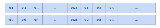
Figure 14. Layout for client point in e2-o0 implementation of distance-64.

The implementations generated by Viaduct-HE make efficient use of the SIMD capabilities of HE with sophisticated layouts. For distance-64, the e1-o0 configuration generates the diagonal layout from Figure 6(b), which reduces the necessary amount of rotations and additions compared to the row-wise baseline layout. The e2-o0 configuration generates an even more efficient layout by using all 2048 vector slots available: the even and odd coordinates of the client point are packed in separate vectors and each coordinate is repeated 64 times, allowing the squared difference of each even (resp. odd) coordinate with the corresponding even (resp. odd) coordinate of each test point to be computed simultaneously. Figure 14 shows the layout for the client point.

Meanwhile, for retrieval-256 the compiler generates a layout where the entire key array and the query are each stored in single vectors. Each bit of the query is repeated 256 times, allowing the equality computation with the corresponding bit of each key to be computed all at once. For retrieval-1024, a similar layout to retrieval-256 is not possible because there are too many keys to store in a single vector. Instead, the e1 configuration explodes the key array bit-wise: each bit of a key is stored in a separate vector, and the corresponding bits of all 1024 keys are packed in the same vector. The e2 configuration, as in distance-64, stores the even and odd bits of keys in separate vectors to use more of the available 8192 vector slots, making it even more efficient.

9.2. Comparison with Expert-written HE Programs

The HE programs generated by the Viaduct-HE compiler are not only dramatically more efficient than the baseline implementations, they also sometimes match or even improve upon expert-written implementations found in the literature.

The conv-simo implementation generated by Viaduct-HE is basically the “packed” convolution kernel defined in Gazelle (Juvekar et al., 2018): both store the image in a single ciphertext, while the values of all 4 filters at a single position are packed in a single plaintext. The image ciphertext is then rotated to align with the filter ciphertexts; since the filter size is 3x3, 9 rotated image ciphertexts and 9 filter plaintexts are multiplied together, and then summed. This computes the convolution for all output pixels at once. The conv-siso implementation is similar, but instead packs columns of the filter into a plaintext instead of single values.

The o1 configurations of conv-siso and conv-simo use algebraic properties of circuits to optimize the implementation further. Given image ciphertext $c$, mask $m$, and plaintext filter $f$, instead of computing $(c\times m)\times f$ in HE as two ciphertext-plaintext operations, circuit optimization rewrites the computation as $c\times(m\times f)$, allowing $m\times f$ to be hoisted out of HE and computed natively. This is exactly the “punctured plaintexts” technique, also from Gazelle.

For double-matmul, Viaduct-HE generates an implementation where each matrix is laid out in a single vector. Importantly, even though $A_{1}$ and $A_{2}$ are both left operands to multiplication, their layouts are different because the layout of $A_{2}$ must account for the output layout of $A_{1}\times B$. The generated implementation is similar to the expert implementation found in Dathathri et al. (2019, Figure 1), but avoids a “clean-and-fill” operation required to derive an empty dimension from a reduced vectorized dimension. The Viaduct-HE implementation avoids this operation by moving the reduced vectorized dimension as the outermost dimension in the vector, thus making it a reduced repeated dimension in the output layout of the first multiplication. The expert implementation takes 0.06 seconds compared to 0.04 seconds taken by the Viaduct-HE implementation, a 1.5x speedup.

Finally, set-union-128 is originally a benchmark for the HECO compiler (Viand et al., 2022). The program computes a mask that zeroes out elements of $B$ with keys that are in $A$, and then adds the sum of values in $A$ with the sum of masked values in $B$. The implementation generated by the HECO compiler is over 40x slower than an expert-written solution: as in the e1 configuration of retrieval-1024, it packs each bit of a key in separate vector, and the corresponding bits of all 128 keys are packed in the same vector. The bits are repeated within each vector such that the computation of masks for all pairs of keys in $A$ and $B$ can be done simultaneously. The Viaduct-HE compiler generates exactly this expert solution.

9.3. Scalability of Compilation

To determine whether the Viaduct-HE compilation process is scalable, we measured the compilation time for each benchmark, with the same scheduling and optimization configurations from RQ1. Figure 13 shows the compilation times for the benchmarks. The two main bottlenecks for compilation are the scheduling and circuit optimization stages, with their sum constituting almost all compilation time.

With 1 epoch, scheduling at most takes 10 seconds; however, with 2 epochs scheduling takes up to 11 minutes (set-union-128). This is because the tiling transformer vastly increases the search space, as it finds many different ways to split dimensions. We find that scheduling is mainly hampered by the fact that circuit generation must be attempted for every visited schedule, as it is currently the only way to determine whether a schedule is valid. In particular, circuit generation is greatly slowed down by array materialization, as in many schedules (especially those with many exploded dimensions), the default array materializer generates thousands of vectors and then tries to derive these vectors from one another, so that scheduler has an accurate count of features such as the number of input vectors and rotations. Speeding up scheduling by estimating such features without array materialization is an interesting research direction.

Meanwhile, circuit optimization time is completely dominated by extraction. In all compilations, equality saturation stops in less than a second, but extraction takes longer (almost 3 minutes for retrieval-256) because the LP extractor must solve an integer linear program.

10. Related Work

Vectorized HE for Specific Applications

There is a large literature on developing efficient vectorized HE implementations of specific applications, particularly for machine learning. Some work such as Cryptonets (Gilad-Bachrach et al., 2016), Gazelle (Juvekar et al., 2018), LoLa (Brutzkus et al., 2019), and HyPHEN (Kim et al., 2023) develop efficient vectorized kernels for neural network inference. Other work such as SEALion (van Elsloo et al., 2019) and nGraph-HE (Boemer et al., 2019b, a) provide domain-specific compilers for neural networks. CHET (Dathathri et al., 2019) automatically selects from a fixed set of data layouts for neural network inference kernels. HeLayers (Aharoni et al., 2023) is similar to CHET in automating layout selection, but can also search for efficient tiling sizes for kernels, akin to the tiling transformer in Viaduct-HE. COPSE (Malik et al., 2021) develops a vectorized implementation of decision forest evaluation.

Compilers for HE

The programmability challenges of HE have inspired much recent work on HE compilers (Viand et al., 2021). HE compilers face similar challenges as compilers for multi-party computation (Hastings et al., 2019; Acay et al., 2021; Rastogi et al., 2014; Büscher et al., 2018; Chen et al., 2023), such as lowering programs to a circuit representation. At the same time, HE has unique programmability challenges that are not comparable to other domains. Some HE compilers such as Alchemy (Crockett et al., 2018), Cingulata (Carpov et al., 2015), EVA (Dathathri et al., 2020), HECATE (Lee et al., 2022), and Ramparts (Archer et al., 2019), focus on other programmability concerns besides vectorization, such as selection of encryption parameters and scheduling “ciphertext maintenance” operations. Lobster (Lee et al., 2020) uses program synthesis and term rewriting to optimize HE circuits, but it focuses on boolean circuits and not on vectorized arithmetic circuits.

Recent work have tackled the challenge of automatically vectorizing programs for HE. Porcupine (Cowan et al., 2021) proposes a synthesis-based approach to generating vectorized HE programs from an imperative source program. However, Porcupine requires the developer to provide the data layout for inputs and can only scale up to HE programs with a small number of instructions. HECO (Viand et al., 2022) attempts to solve the scalability issue by analyzing indexing operations in the source program in lieu of program synthesis, but fixes a simple layout for all programs, leaving many optimization opportunities out of reach. Coyote (Malik et al., 2023) uses search and LP to find efficient vectorizations of arithmetic circuits, balancing vectorization opportunities with data movement costs. Coyote can vectorize “irregular” programs that are out of scope for Viaduct-HE. At the same time, though it can generate layouts for HE programs, Coyote still requires user hints for “noncanonical” layouts. Also, Coyote appears to be less scalable than Viaduct-HE, as compiling a 16x16 matrix multiplication requires decomposition into 4x4 matrices that are “blocked” together.

Array-oriented Languages

In the taxonomy given by Paszke et al. (2021), the Viaduct-HE source language is a “pointful” array-oriented language with explicit indexing constructs, in contrast to array “combinator” languages such as Futhark (Henriksen et al., 2017) and Lift (Steuwer et al., 2017). The Viaduct-HE source language is thus similar in spirit to languages such as ATL (Bernstein et al., 2020; Liu et al., 2022), Dex (Paszke et al., 2021), and Tensor Comprehensions (Vasilache et al., 2018). In particular, the separation of algorithm and schedule in Viaduct-HE is inspired by the Halide (Ragan-Kelley et al., 2013) language and compiler for image processing pipelines. Although the source language of Viaduct-HE is similar to Halide’s—both are pointful array languages—Viaduct-HE schedules have very different concerns from Halide schedules. On one hand, Halide schedules represent choices such as what order the values of an image processing stage should be computed, and the granularity at which stage results are stored; on the other hand, Viaduct-HE schedules represent the layout of data in ciphertext and plaintext vectors.

11. Summary

With its array-oriented source language, the Viaduct-HE compiler can give a simple representation for vectorization schedules and find sophisticated data layouts comparable to expert HE implementations. The compiler also has representations to allow for algebraic optimizations and for easy implementation of back ends for new HE libraries. Overall, the Viaduct-HE compiler drastically lowers the programmability burden of vectorized homomorphic encryption.

References

- (1)
- Acay et al. (2021) Coşku Acay, Rolph Recto, Joshua Gancher, Andrew Myers, and Elaine Shi. 2021. Viaduct: An Extensible, Optimizing Compiler for Secure Distributed Programs. In 42nd ACM SIGPLAN Conf. on Programming Language Design and Implementation (PLDI). https://doi.org/10.1145/3453483.3454074
- Aharoni et al. (2023) Ehud Aharoni, Allon Adir, Moran Baruch, Nir Drucker, Gilad Ezov, Ariel Farkash, Lev Greenberg, Ramy Masalha, Guy Moshkowich, Dov Murik, Hayim Shaul, and Omri Soceanu. 2023. HeLayers: A Tile Tensors Framework for Large Neural Networks on Encrypted Data. Proc. Priv. Enhancing Technol. 2023, 1 (2023), 325–342. https://doi.org/10.56553/popets-2023-0020
- Albrecht et al. (2018) Martin Albrecht, Melissa Chase, Hao Chen, Jintai Ding, Shafi Goldwasser, Sergey Gorbunov, Shai Halevi, Jeffrey Hoffstein, Kim Laine, Kristin Lauter, Satya Lokam, Daniele Micciancio, Dustin Moody, Travis Morrison, Amit Sahai, and Vinod Vaikuntanathan. 2018. Homomorphic Encryption Security Standard. Technical Report. HomomorphicEncryption.org, Toronto, Canada.
- Archer et al. (2019) David W Archer, José Manuel Calderón Trilla, Jason Dagit, Alex Malozemoff, Yuriy Polyakov, Kurt Rohloff, and Gerard Ryan. 2019. Ramparts: A programmer-friendly system for building homomorphic encryption applications. In Proceedings of the 7th ACM Workshop on Encrypted Computing & Applied Homomorphic Cryptography. 57–68.
- Bernstein et al. (2020) Gilbert Bernstein, Michael Mara, Tzu-Mao Li, Dougal Maclaurin, and Jonathan Ragan-Kelley. 2020. Differentiating a Tensor Language. CoRR abs/2008.11256 (2020). arXiv:2008.11256
- Boemer et al. (2019a) Fabian Boemer, Anamaria Costache, Rosario Cammarota, and Casimir Wierzynski. 2019a. nGraph-HE2: A High-Throughput Framework for Neural Network Inference on Encrypted Data. In Proceedings of the 7th ACM Workshop on Encrypted Computing & Applied Homomorphic Cryptography, WAHC@CCS 2019, London, UK, November 11-15, 2019, Michael Brenner, Tancrède Lepoint, and Kurt Rohloff (Eds.). ACM, 45–56. https://doi.org/10.1145/3338469.3358944
- Boemer et al. (2019b) Fabian Boemer, Yixing Lao, Rosario Cammarota, and Casimir Wierzynski. 2019b. nGraph-HE: a graph compiler for deep learning on homomorphically encrypted data. In Proceedings of the 16th ACM International Conference on Computing Frontiers, CF 2019, Alghero, Italy, April 30 - May 2, 2019, Francesca Palumbo, Michela Becchi, Martin Schulz, and Kento Sato (Eds.). ACM, 3–13. https://doi.org/10.1145/3310273.3323047
- Brakerski et al. (2014) Zvika Brakerski, Craig Gentry, and Vinod Vaikuntanathan. 2014. (Leveled) fully homomorphic encryption without bootstrapping. ACM Transactions on Computation Theory (TOCT) 6, 3 (2014), 1–36.
- Brutzkus et al. (2019) Alon Brutzkus, Ran Gilad-Bachrach, and Oren Elisha. 2019. Low Latency Privacy Preserving Inference. In Proceedings of the 36th International Conference on Machine Learning, ICML 2019, 9-15 June 2019, Long Beach, California, USA (Proceedings of Machine Learning Research, Vol. 97), Kamalika Chaudhuri and Ruslan Salakhutdinov (Eds.). PMLR, 812–821.
- Büscher et al. (2018) Niklas Büscher, Daniel Demmler, Stefan Katzenbeisser, David Kretzmer, and Thomas Schneider. 2018. HyCC: Compilation of Hybrid Protocols for Practical Secure Computation. In 25th ACM Conf. on Computer and Communications Security (CCS). ACM, New York, NY, USA, 847–861. https://doi.org/10.1145/3243734.3243786
- Carpov et al. (2015) Sergiu Carpov, Paul Dubrulle, and Renaud Sirdey. 2015. Armadillo: a compilation chain for privacy preserving applications. In Proceedings of the 3rd International Workshop on Security in Cloud Computing. 13–19.
- Chen et al. (2023) Edward Chen, Jinhao Zhu, Alex Ozdemir, Riad S Wahby, Fraser Brown, and Wenting Zheng. 2023. Silph: A Framework for Scalable and Accurate Generation of Hybrid MPC Protocols. Cryptology ePrint Archive (2023).
- Chen et al. (2017) Hao Chen, Kim Laine, and Rachel Player. 2017. Simple encrypted arithmetic library-SEAL v2. 1. In Financial Cryptography and Data Security: FC 2017 International Workshops, WAHC, BITCOIN, VOTING, WTSC, and TA, Sliema, Malta, April 7, 2017, Revised Selected Papers 21. Springer, 3–18.
- Cheon et al. (2017) Jung Hee Cheon, Andrey Kim, Miran Kim, and Yongsoo Song. 2017. Homomorphic encryption for arithmetic of approximate numbers. In Advances in Cryptology–ASIACRYPT 2017: 23rd International Conference on the Theory and Applications of Cryptology and Information Security, Hong Kong, China, December 3-7, 2017, Proceedings, Part I 23. Springer, 409–437.
- COIN-OR (4 11) COIN-OR. accessed 2023-04-11. Cbc - COIN-OR Branch and Cut. https://www.coin-or.org/Cbc/.
- Cowan et al. (2021) Meghan Cowan, Deeksha Dangwal, Armin Alaghi, Caroline Trippel, Vincent T. Lee, and Brandon Reagen. 2021. Porcupine: A Synthesizing Compiler for Vectorized Homomorphic Encryption. In 42nd ACM SIGPLAN Conf. on Programming Language Design and Implementation (PLDI), Stephen N. Freund and Eran Yahav (Eds.). ACM, 375–389. https://doi.org/10.1145/3453483.3454050
- Crockett et al. (2018) Eric Crockett, Chris Peikert, and Chad Sharp. 2018. Alchemy: A language and compiler for homomorphic encryption made easy. In Proceedings of the 2018 ACM SIGSAC Conference on Computer and Communications Security. 1020–1037.
- Dathathri et al. (2020) Roshan Dathathri, Blagovesta Kostova, Olli Saarikivi, Wei Dai, Kim Laine, and Madan Musuvathi. 2020. EVA: An Encrypted Vector Arithmetic Language and Compiler for Efficient Homomorphic Computation. In 41st ACM SIGPLAN Conf. on Programming Language Design and Implementation (PLDI), Alastair F. Donaldson and Emina Torlak (Eds.). ACM, 546–561. https://doi.org/10.1145/3385412.3386023
- Dathathri et al. (2019) Roshan Dathathri, Olli Saarikivi, Hao Chen, Kim Laine, Kristin E. Lauter, Saeed Maleki, Madanlal Musuvathi, and Todd Mytkowicz. 2019. CHET: An Optimizing Compiler for Fully-Homomorphic Neural-Network Inferencing. In 40th ACM SIGPLAN Conf. on Programming Language Design and Implementation (PLDI), Kathryn S. McKinley and Kathleen Fisher (Eds.). ACM, 142–156. https://doi.org/10.1145/3314221.3314628
- Fan and Vercauteren (2012) Junfeng Fan and Frederik Vercauteren. 2012. Somewhat practical fully homomorphic encryption. Cryptology ePrint Archive (2012).
- Gilad-Bachrach et al. (2016) Ran Gilad-Bachrach, Nathan Dowlin, Kim Laine, Kristin Lauter, Michael Naehrig, and John Wernsing. 2016. Cryptonets: Applying neural networks to encrypted data with high throughput and accuracy. In International conference on machine learning. PMLR, 201–210.
- Halevi and Shoup (2014) Shai Halevi and Victor Shoup. 2014. Algorithms in HElib. In Advances in Cryptology - CRYPTO 2014 - 34th Annual Cryptology Conference, Santa Barbara, CA, USA, August 17-21, 2014, Proceedings, Part I (Lecture Notes in Computer Science, Vol. 8616), Juan A. Garay and Rosario Gennaro (Eds.). Springer, 554–571. https://doi.org/10.1007/978-3-662-44371-2_31
- Harris et al. (2020) Charles R. Harris, K. Jarrod Millman, Stéfan J. van der Walt, Ralf Gommers, Pauli Virtanen, David Cournapeau, Eric Wieser, Julian Taylor, Sebastian Berg, Nathaniel J. Smith, Robert Kern, Matti Picus, Stephan Hoyer, Marten H. van Kerkwijk, Matthew Brett, Allan Haldane, Jaime Fernández del Río, Mark Wiebe, Pearu Peterson, Pierre Gérard-Marchant, Kevin Sheppard, Tyler Reddy, Warren Weckesser, Hameer Abbasi, Christoph Gohlke, and Travis E. Oliphant. 2020. Array programming with NumPy. Nature 585, 7825 (Sept. 2020), 357–362. https://doi.org/10.1038/s41586-020-2649-2
- Hastings et al. (2019) Marcella Hastings, Brett Hemenway, Daniel Noble, and Steve Zdancewic. 2019. SoK: General Purpose Compilers for Secure Multi-Party Computation. In IEEE Symp. on Security and Privacy. 1220–1237. https://doi.org/10.1109/SP.2019.00028
- Henriksen et al. (2017) Troels Henriksen, Niels G. W. Serup, Martin Elsman, Fritz Henglein, and Cosmin E. Oancea. 2017. Futhark: Purely Functional GPU-Programming with Nested Parallelism and in-Place Array Updates. SIGPLAN Not. 52, 6 (jun 2017), 556–571. https://doi.org/10.1145/3140587.3062354
- Juvekar et al. (2018) Chiraag Juvekar, Vinod Vaikuntanathan, and Anantha P. Chandrakasan. 2018. GAZELLE: A Low Latency Framework for Secure Neural Network Inference. In 27th USENIX Security Symposium, USENIX Security 2018, Baltimore, MD, USA, August 15-17, 2018, William Enck and Adrienne Porter Felt (Eds.). USENIX Association, 1651–1669.
- Kim et al. (2023) Donghwan Kim, Jaiyoung Park, Jongmin Kim, Sangpyo Kim, and Jung Ho Ahn. 2023. HyPHEN: A Hybrid Packing Method and Optimizations for Homomorphic Encryption-Based Neural Networks. CoRR abs/2302.02407 (2023). https://doi.org/10.48550/arXiv.2302.02407 arXiv:2302.02407
- Kim et al. (2021) Miran Kim, Arif Ozgun Harmanci, Jean-Philippe Bossuat, Sergiu Carpov, Jung Hee Cheon, Ilaria Chillotti, Wonhee Cho, David Froelicher, Nicolas Gama, Mariya Georgieva, et al. 2021. Ultrafast homomorphic encryption models enable secure outsourcing of genotype imputation. Cell systems 12, 11 (2021), 1108–1120.
- Lauter et al. (2021) Kristin Lauter, Sreekanth Kannepalli, Kim Laine, and Radames Cruz Moreno. 2021. Password Monitor: Safeguarding passwords in Microsoft Edge.
- Lee et al. (2020) DongKwon Lee, Woosuk Lee, Hakjoo Oh, and Kwangkeun Yi. 2020. Optimizing homomorphic evaluation circuits by program synthesis and term rewriting. In Proceedings of the 41st ACM SIGPLAN Conference on Programming Language Design and Implementation. 503–518.
- Lee et al. (2022) Yongwoo Lee, Seonyeong Heo, Seonyoung Cheon, Shinnung Jeong, Changsu Kim, Eunkyung Kim, Dongyoon Lee, and Hanjun Kim. 2022. HECATE: Performance-Aware Scale Optimization for Homomorphic Encryption Compiler. In IEEE/ACM International Symposium on Code Generation and Optimization, CGO 2022, Seoul, Korea, Republic of, April 2-6, 2022, Jae W. Lee, Sebastian Hack, and Tatiana Shpeisman (Eds.). IEEE, 193–204. https://doi.org/10.1109/CGO53902.2022.9741265
- Liu et al. (2022) Amanda Liu, Gilbert Louis Bernstein, Adam Chlipala, and Jonathan Ragan-Kelley. 2022. Verified tensor-program optimization via high-level scheduling rewrites. Proc. ACM Program. Lang. 6, POPL (2022), 1–28. https://doi.org/10.1145/3498717
- Malik et al. (2023) Raghav Malik, Kabir Sheth, and Milind Kulkarni. 2023. Coyote: A Compiler for Vectorizing Encrypted Arithmetic Circuits. In Proceedings of the 28th ACM International Conference on Architectural Support for Programming Languages and Operating Systems, Volume 3. 118–133.
- Malik et al. (2021) Raghav Malik, Vidush Singhal, Benjamin Gottfried, and Milind Kulkarni. 2021. Vectorized secure evaluation of decision forests. In 42nd ACM SIGPLAN Conf. on Programming Language Design and Implementation (PLDI), Stephen N. Freund and Eran Yahav (Eds.). ACM, 1049–1063. https://doi.org/10.1145/3453483.3454094
- Menon and Wu (2022) Samir Jordan Menon and David J Wu. 2022. Spiral: Fast, high-rate single-server PIR via FHE composition. In 2022 IEEE Symposium on Security and Privacy (SP). IEEE, 930–947.
- Paszke et al. (2021) Adam Paszke, Daniel D. Johnson, David Duvenaud, Dimitrios Vytiniotis, Alexey Radul, Matthew J. Johnson, Jonathan Ragan-Kelley, and Dougal Maclaurin. 2021. Getting to the point: index sets and parallelism-preserving autodiff for pointful array programming. Proc. ACM Program. Lang. 5, ICFP (2021), 1–29. https://doi.org/10.1145/3473593
- Ragan-Kelley et al. (2013) Jonathan Ragan-Kelley, Connelly Barnes, Andrew Adams, Sylvain Paris, Frédo Durand, and Saman P. Amarasinghe. 2013. Halide: a language and compiler for optimizing parallelism, locality, and recomputation in image processing pipelines. In ACM SIGPLAN Conference on Programming Language Design and Implementation, PLDI ’13, Seattle, WA, USA, June 16-19, 2013, Hans-Juergen Boehm and Cormac Flanagan (Eds.). ACM, 519–530. https://doi.org/10.1145/2491956.2462176
- Rastogi et al. (2014) Aseem Rastogi, Matthew A. Hammer, and Michael Hicks. 2014. Wysteria: A Programming Language for Generic, Mixed-Mode Multiparty Computations. In IEEE Symp. on Security and Privacy. 655–670. https://doi.org/10.1109/SP.2014.48
- Reagen et al. (2021) Brandon Reagen, Woo-Seok Choi, Yeongil Ko, Vincent T Lee, Hsien-Hsin S Lee, Gu-Yeon Wei, and David Brooks. 2021. Cheetah: Optimizing and accelerating homomorphic encryption for private inference. In 2021 IEEE International Symposium on High-Performance Computer Architecture (HPCA). IEEE, 26–39.
- Riazi et al. (2020) M Sadegh Riazi, Kim Laine, Blake Pelton, and Wei Dai. 2020. HEAX: An architecture for computing on encrypted data. In Proceedings of the Twenty-Fifth International Conference on Architectural Support for Programming Languages and Operating Systems. 1295–1309.
- Steuwer et al. (2017) Michel Steuwer, Toomas Remmelg, and Christophe Dubach. 2017. Lift: a functional data-parallel IR for high-performance GPU code generation. In Proceedings of the 2017 International Symposium on Code Generation and Optimization, CGO 2017, Austin, TX, USA, February 4-8, 2017, Vijay Janapa Reddi, Aaron Smith, and Lingjia Tang (Eds.). ACM, 74–85.
- Tate et al. (2009) Ross Tate, Michael Stepp, Zachary Tatlock, and Sorin Lerner. 2009. Equality saturation: a new approach to optimization. In Proceedings of the 36th ACM SIGPLAN-SIGACT Symposium on Principles of Programming Languages, POPL 2009, Savannah, GA, USA, January 21-23, 2009, Zhong Shao and Benjamin C. Pierce (Eds.). ACM, 264–276. https://doi.org/10.1145/1480881.1480915
- Titus et al. (2018) Alexander J Titus, Shashwat Kishore, Todd Stavish, Stephanie M Rogers, and Karl Ni. 2018. PySEAL: A Python wrapper implementation of the SEAL homomorphic encryption library. arXiv preprint arXiv:1803.01891 (2018).
- van Elsloo et al. (2019) Tim van Elsloo, Giorgio Patrini, and Hamish Ivey-Law. 2019. SEALion: a Framework for Neural Network Inference on Encrypted Data. CoRR abs/1904.12840 (2019). arXiv:1904.12840
- Vasilache et al. (2018) Nicolas Vasilache, Oleksandr Zinenko, Theodoros Theodoridis, Priya Goyal, Zachary DeVito, William S. Moses, Sven Verdoolaege, Andrew Adams, and Albert Cohen. 2018. Tensor Comprehensions: Framework-Agnostic High-Performance Machine Learning Abstractions. CoRR abs/1802.04730 (2018). arXiv:1802.04730
- Viand et al. (2022) Alexander Viand, Patrick Jattke, Miro Haller, and Anwar Hithnawi. 2022. HECO: Automatic Code Optimizations for Efficient Fully Homomorphic Encryption. CoRR abs/2202.01649 (2022). arXiv:2202.01649
- Viand et al. (2021) Alexander Viand, Patrick Jattke, and Anwar Hithnawi. 2021. SoK: Fully Homomorphic Encryption Compilers. In 42nd IEEE Symposium on Security and Privacy, SP 2021, San Francisco, CA, USA, 24-27 May 2021. IEEE, 1092–1108. https://doi.org/10.1109/SP40001.2021.00068
- Willsey et al. (2021) Max Willsey, Chandrakana Nandi, Yisu Remy Wang, Oliver Flatt, Zachary Tatlock, and Pavel Panchekha. 2021. Egg: Fast and Extensible Equality Saturation. Proc. ACM Program. Lang. 5, POPL, Article 23 (jan 2021), 29 pages. https://doi.org/10.1145/3434304