SMEFT at NNLO+PS: $Vh$ production

Abstract

In the context of the Standard Model effective field theory (SMEFT) the next-to-next-to-leading (NNLO) QCD corrections to the Higgsstrahlungs ($Vh$) processes in hadronic collisions are calculated and matched to a parton shower (PS). NNLO+PS precision is achieved for the complete sets of SMEFT operators that describe the interactions between the Higgs and two vector bosons and the couplings of the Higgs, a $W$ or a $Z$ boson, and light fermions. A POWHEG-BOX implementation of the computed NNLO SMEFT corrections is provided that allows for a realistic exclusive description of $Vh$ production at the level of hadronic events. This feature makes it an essential tool for future Higgs characterisation studies by the ATLAS and CMS collaborations. Utilising our new Monte Carlo code the numerical impact of NNLO$+$PS corrections on the kinematic distributions in $pp\to Zh\to\ell^{+}\ell^{-}h$ production is explored, employing well-motivated SMEFT benchmark scenarios.

1 Introduction

The dominant decay of the Standard Model (SM) Higgs boson is into a pair of bottom quarks, with an expected branching ratio close to 60% for a Higgs mass of $125\,{\rm GeV}$. Large QCD backgrounds from multi-jet production, however, make a search in the dominant gluon-gluon fusion (ggF) Higgs production channel very challenging at the LHC. The most sensitive production mode for detecting $h\to b\bar{b}$ decays is the associated production of a Higgs boson and a massive gauge boson ($Vh$), where the leptonic decay of the vector boson enables a clean selection, leading to a significant background reduction. The $h\to b\bar{b}$ decay mode has been observed by both ATLAS and CMS in LHC Run II ATLAS:2018kot ; CMS:2018nsn , and these measurements constrain the $h\to b\bar{b}$ signal strength in the Higgsstrahlungs processes $\big{(}\mu^{b\bar{b}}_{Vh}\big{)}$ to be SM-like within about 25%. With LHC Run III ongoing and the high-luminosity upgrade (HL-LHC) on the horizon, the precision of the $\mu^{b\bar{b}}_{Vh}$ measurements is expected to improve significantly, resulting in an ultimate projected HL-LHC accuracy of $15\%$ ($5\%$) in the case of the $Wh$ ($Zh)$ production channel ATLAS:2018jlh ; CMS:2018qgz .

Besides providing a probe of the dominant decay mode of the Higgs boson, precision $Vh$ measurements also play an important role in the Higgs characterisation programme which is commonly performed in the framework of the SM effective field theory (SMEFT) Buchmuller:1985jz ; Grzadkowski:2010es ; Brivio:2017vri . In fact, radiative corrections in the SMEFT to both $Vh$ production Mimasu:2015nqa ; Degrande:2016dqg ; Alioli:2018ljm ; Bishara:2020vix ; Bishara:2020pfx ; Bishara:2022vsc and the $h\to f\bar{f}$ decays Gauld:2015lmb ; Gauld:2016kuu ; Cullen:2019nnr ; Cullen:2020zof ; Haisch:2022nwz have been calculated. The existing studies for $Vh$ production have mostly focused on the subset of higher-dimensional interactions that modify the couplings of the Higgs to two vector bosons achieving next-to-leading order (NLO) Maltoni:2013sma ; Mimasu:2015nqa ; Degrande:2016dqg ; Greljo:2017spw ; Alioli:2018ljm and next-to-next-to-leading order (NNLO) Bizon:2021rww in QCD, respectively, while in the case of $h\to b\bar{b}$ both NLO QCD and NLO electroweak (EW) corrections to the total decay width have been calculated for the full set of relevant dimension-six SMEFT operators Gauld:2015lmb ; Gauld:2016kuu ; Cullen:2019nnr . In the publications Bishara:2020vix ; Bishara:2020pfx ; Bishara:2022vsc special attention has finally been paid to the class of SMEFT operators that lead to interactions between a Higgs, $W$ or $Z$ boson, and light quarks.

The goal of the present work is to generalise and to extend the recent SMEFT calculation Haisch:2022nwz which has achieved NNLO plus parton shower (NNLO$+$PS) accuracy for the dimension-six operators that contribute to the subprocesses $pp\to Zh$ and $h\to b\bar{b}$ directly in QCD. This class of operators includes effective Yukawa- and chromomagnetic dipole-type interactions of the bottom quark that modify the $h\to b\bar{b}$ decay but do not play a role in $pp\to Zh$ production. Purely EW effective interactions that alter the couplings of the Higgs to gauge bosons are instead not included in the NNLO$+$PS Monte Carlo (MC) generator presented in Haisch:2022nwz . Since these types of SMEFT contributions can lead to phenomenologically relevant effects in the Higgsstrahlungs processes Maltoni:2013sma ; Mimasu:2015nqa ; Degrande:2016dqg ; Greljo:2017spw ; Alioli:2018ljm ; Bizon:2021rww , we include these type of interactions in the current article, extending the NLO SMEFT calculations Mimasu:2015nqa ; Degrande:2016dqg ; Alioli:2018ljm to the NNLO level. Likewise, we improve the precision of the calculations of SMEFT corrections to $pp\to Vh$ production that are associated to couplings between a Higgs, $W$ or $Z$ boson, and light quarks Bishara:2020vix ; Bishara:2020pfx ; Bishara:2022vsc to NNLO in QCD. The obtained fixed-order SMEFT predictions are implemented into the POWHEG-BOX Alioli:2010xd and consistently matched to a parton shower (PS) using the MiNNLO_PS method Monni:2019whf ; Monni:2020nks . In this way, NNLO QCD accuracy is retained for both production and decays, while the matching to the PS ensures a realistic exclusive description of the $pp\to Zh\to\ell^{+}\ell^{-}h$ and the $pp\to Wh\to\ell\nu h$ process at the level of hadronic events. These features make our new NNLO$+$PS generator a precision tool for future LHC Higgs characterisation studies in the SMEFT framework.

This paper is structured as follows: in Section 2 we specify the dimension-six SMEFT operators that are relevant in the context of our work. A comprehensive description of the basic ingredients of the SMEFT calculation of $pp\to Vh$ production and their implementation in the context of our NNLO$+$PS event generator is presented in Section 3. We motivate simple SMEFT benchmark scenarios in Section 4 by discussing the leading constraints on the Wilson coefficients of the relevant operators. The impact of the SMEFT corrections on kinematic distributions in $pp\to Zh\to\ell^{+}\ell^{-}h$ production at the LHC is studied in Section 5 employing the simple benchmark scenarios for the Wilson coefficients identified earlier. In Section 6 we outline how the NNLO$+$PS calculations of $pp\to Vh$ and $h\to b\bar{b}$ can be combined, while Section 7 contains our conclusions and an outlook. The analytic formulae for the parameters and couplings that have been implemented into our MC code are relegated to Appendix A. Details on our implementation of the $gg\to Zh$ process can be found in Appendix B. In Appendix C we finally discuss the impact of NNLO QCD effects by comparing results for $pp\to Zh\to\ell^{+}\ell^{-}h$ production obtained at NLO$+$PS and NNLO$+$PS, respectively.

2 SMEFT operators

Throughout this work we neglect all light fermion masses in both the SM and SMEFT corrections to the $pp\to Zh$ and $pp\to Wh$ processes. The full set of dimension-six SMEFT operators has been presented in the so-called Warsaw basis in the article Grzadkowski:2010es . This basis contains the following three independent operators

$$Q_{HB}=H^{\dagger}H\hskip 1.42262ptB_{\mu\nu}B^{\mu\nu}\,,\quad Q_{HW}=H^{\dagger}H\hskip 1.42262ptW_{\mu\nu}^{a}W^{a,\mu\nu}\,,\quad Q_{HW\!B}=H^{\dagger}\sigma^{a}H\hskip 1.42262ptW_{\mu\nu}^{a}B^{\mu\nu}\,,$$ (1)

that modify the couplings between the Higgs and two vector bosons at tree level. The SM Higgs doublet is denoted by $H$, while $B_{\mu\nu}$ and $W_{\mu\nu}^{a}$ are the $U(1)_{Y}$ and $SU(2)_{L}$ gauge field strength tensors and $\sigma^{a}$ are the Pauli matrices. In the case of the operators that result in couplings between the Higgs, a $W$ or a $Z$ boson, and light quarks, we consider the following four effective interactions

$$\begin{split}&Q_{Hq}^{(1)}=(H^{\dagger}i\overset{\leftrightarrow}{D}_{\mu}H)(\bar{q}\gamma^{\mu}q)\,,\qquad Q_{Hq}^{(3)}=(H^{\dagger}i\overset{\leftrightarrow}{D}\ \!\!\!^{\;a}_{\mu}H)(\bar{q}\gamma^{\mu}\sigma^{a}q)\,,\\[2.84526pt] &\hskip 2.84526ptQ_{Hd}=(H^{\dagger}i\overset{\leftrightarrow}{D}_{\mu}H)(\bar{d}\gamma^{\mu}d)\,,\qquad Q_{Hu}=(H^{\dagger}i\overset{\leftrightarrow}{D}_{\mu}H)(\bar{u}\gamma^{\mu}u)\,,\end{split}$$ (2)

where $H^{\dagger}i\overset{\leftrightarrow}{D}_{\mu}H=iH^{\dagger}\big{(}D_{\mu}-\overset{\leftarrow}{D}_{\mu}\big{)}H$ and $H^{\dagger}i\overset{\leftrightarrow}{D}\ \!\!\!^{\;a}_{\mu}H=iH^{\dagger}\big{(}\sigma^{a}D_{\mu}-\overset{\leftarrow}{D}_{\mu}\sigma^{a}\big{)}H$ with $D_{\mu}$ the usual covariant derivative. The symbol $q$ denotes left-handed quark doublets, while $u$ and $d$ are the right-handed quark singlets of up and down type, respectively. Illustrative diagrams that contribute to $Zh$ production and involve an insertion of one of the operators in (1) or (2) are displayed in Figure 1.

Besides the two sets of operators (1) and (2) that alter the $pp\to Vh$ production process, we also consider effective interactions that modify the $Z\to\ell^{+}\ell^{-}$ and $W\to\ell\nu$ decays at tree level. In the Warsaw basis there are three such operators, namely

$$Q_{H\ell}^{(1)}=(H^{\dagger}i\overset{\leftrightarrow}{D}_{\mu}H)(\bar{\ell}\gamma^{\mu}\ell)\,,\quad Q_{H\ell}^{(3)}=(H^{\dagger}i\overset{\leftrightarrow}{D}\ \!\!\!^{\;a}_{\mu}H)(\bar{\ell}\gamma^{\mu}\sigma^{a}\ell)\,,\quad Q_{He}=(H^{\dagger}i\overset{\leftrightarrow}{D}_{\mu}H)(\bar{e}\gamma^{\mu}e)\,.\hskip 17.07164pt$$ (3)

Here $\ell$ and $e$ denote a left-handed lepton doublet and right-handed lepton singlet field, respectively. Notice that in writing (2) and (3) we have assumed that the full SMEFT Lagrangian respects an approximate $U(3)^{5}$ flavour symmetry which allows us to drop all flavour indices.

The final type of SMEFT corrections that change the Higgsstrahlungs processes indirectly is provided by the Wilson coefficients of the operators that shift the Higgs kinetic term and/or the EW SM input parameters. In order to fully describe these shifts the following three additional operators are needed at tree level:

$$Q_{H\Box}=(H^{\dagger}H)\Box(H^{\dagger}H)\,,\quad Q_{HD}=(H^{\dagger}D_{\mu}H)^{\ast}(H^{\dagger}D^{\mu}H)\,,\quad Q_{\ell\ell}=(\bar{\ell}\gamma_{\mu}\ell)(\bar{\ell}\gamma^{\mu}\ell)\,.$$ (4)

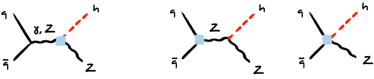
Figure 1: Tree-level SMEFT contributions to $q\bar{q}\to Zh$ production. The diagram on the left involves an insertion of one of the operators defined in (1), while the two graphs on the right stem from an insertion of one of the operators given in (2). The operator insertions are indicated by the blue squares.

3 Calculation in a nutshell

In this section, we sketch the different ingredients of our NNLO$+$PS SMEFT calculation of $pp\to Vh$ production. We begin by recalling the basic steps of the NNLO QCD computation within the SM and then detail the general method that we employ to calculate the relevant squared matrix elements in the SMEFT and their implementation into the POWHEG-BOX. It is then explained how the fixed-order NNLO SMEFT calculations of the $pp\to Vh$ processes are consistently matched to a PS using the MiNNLO_PS method.

3.1 SM calculation

A core input of the NNLO QCD calculation are the squared matrix elements up to $\mathcal{O}(\alpha_{s}^{2})$ in the SMEFT. To better explain how the calculation of these objects is performed, we first revisit the structure of the NNLO computation in the SM, which we have repeated, and also implemented into the POWHEG-BOX. Before doing so, we note that we will generically refer to the process $pp\to Vh$ (and its corresponding subprocesses) in both the text and corresponding figures in what follows, but it should be understood that $V=W,Z$ refers to a final-state lepton pair, and that the calculation does include spin-correlation effects in the gauge-boson decays.

In the NNLO calculation of $pp\to Vh$, the contributing partonic channels can be classified according to the number of external quark lines ($\texttt{A}=0,\texttt{B}=1,\texttt{C}=\texttt{D}=2$), external gluons, and also by the number of loops at the squared amplitude level — see also Majer:2020kdg . Starting with the B-type corrections (i.e. those with a single external quark line), the required squared matrix elements are called B0g0V, B1g0V, B0g1V, B1g1V, B2g0V, B0g2V, where the number before g refers to the number of additional external gluons relative to the leading-order (LO) contribution for that type, and the number after the g refers to the number of loops at the squared level. For example, the left most diagram in Figure 2 contains one additional gluon (relative to the Born-level contribution in the quark-antiquark fusion or ${\rm q\bar{q}F}$ channel) and is a one-loop graph, and would therefore contribute to B1g1V through interference with the corresponding tree-level amplitude. In the case of the SM, the analytic expressions for the corresponding spinor-helicity amplitudes can be found in Kramer:1986sg ; Hamberg:1990np ; Gehrmann:2011ab ; Majer:2020kdg . To obtain the desired squared matrix elements, the spinor-helicity amplitudes can be squared and then summed over all contributing helicities numerically — an explicit example of this procedure is given below. The C-type corrections feature two external quarks lines, or in other words a double real emission contribution with two final-state quarks, and arise from the interference of diagrams such as that represented in the centre of Figure 2. The D-type corrections account for the additional structures that can appear when same-flavour quarks are considered. These squared matrix elements are called C0g0V and D0g0V and within the SM the analytic expressions for the corresponding spinor-helicity amplitudes are provided in the work Majer:2020kdg . Finally, the ggF contributions shown on the right in Figure 2 constitute the third type of correction which are considered (A-type). They are referred to as A0g2V and the corresponding SM spinor-helicity amplitudes are given in Campbell:2016jau . Notice that due to charge conservation the third type of corrections only contributes to the $pp\to Zh$ but not the $pp\to Wh$ process. We add that the corrections called $V_{I,II}$ and $R_{I,II}$ that are related to top-quark loops and involve one external quark line Brein:2011vx are neglected in our SM calculation. Since in total the numerical effect of these contributions amounts to only around $1\%$ Brein:2011vx ; Zanoli:2021iyp ; Haisch:2022nwz , ignoring the $V_{I,II}$ and $R_{I,II}$ terms seems justified at present.

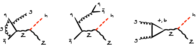
Figure 2: Examples of higher-order QCD corrections to $pp\to Zh$ production within the SM. The diagram on the left features additional virtual and real gluon lines (B-type), the diagram in the middle involves a second quark line (C- and D-type) and the diagram on the right is a ggF contribution (A-type). Consult the main text for further details.

The corresponding calculation including the impact of SMEFT operators (which will be discussed in the following subsection) can also be performed using spinor-helicity techniques. That calculation requires new helicity amplitudes which can (in part) be obtained from knowledge of the SM amplitudes. For clarity of explanation, it will be useful to first consider an explicit example in the SM. To do that we consider the case of B1g0Z which involves a single external quark line and one external gluon at tree level. A corresponding SM Feynman diagram is displayed on the left-hand side in Figure 3. Note that we consider the leptons (quarks) to be outgoing (incoming). The corresponding spinor-helicity amplitude with left-handed fermion chiralities and a physical gluon with a negative helicity reads

$${\cal A}_{\texttt{B1g0Z}}\left(1_{q}^{-},2_{g}^{-},3^{+}_{\bar{q}};4_{\ell}^{-},5_{\bar{\ell}}^{+}\right)=\frac{\braket{34}}{\braket{12}\braket{23}}\Big{(}\braket{13}\left[51\right]+\braket{23}\left[52\right]\Big{)}\,,$$ (5)

where $\braket{ij}$ and $[ij]$ denote the usual spinor products — see for example Dixon:1996wi for a review of the spinor-helicity formalism. Notice that the semicolon in the expression on the left-hand side of (5) separates the particles with incoming and outgoing convention, respectively. The amplitudes for the remaining helicity combinations can be obtained via the following parity and charge conjugation relations

$$\begin{split}{\cal A}_{\texttt{B1g0Z}}\left(1_{q}^{-},2_{g}^{+},3^{+}_{\bar{q}};4_{\ell}^{-},5_{\bar{\ell}}^{+}\right)&=-{\cal A}_{\texttt{B1g0Z}}\left(3_{q}^{-},2_{g}^{-},1^{+}_{\bar{q}};5_{\ell}^{-},4_{\bar{\ell}}^{+}\right)^{*}\,,\\[5.69054pt] {\cal A}_{\texttt{B1g0Z}}\left(1_{q}^{-},2_{g}^{h_{g}},3^{+}_{\bar{q}};4_{\ell}^{+},5_{\bar{\ell}}^{-}\right)&={\cal A}_{\texttt{B1g0Z}}\left(1_{q}^{-},2_{g}^{h_{g}},3^{+}_{\bar{q}};5_{\ell}^{-},4_{\bar{\ell}}^{+}\right)\,,\\[5.69054pt] {\cal A}_{\texttt{B1g0Z}}\left(1_{q}^{+},2_{g}^{h_{g}},3^{-}_{\bar{q}};4_{\ell}^{-},5_{\bar{\ell}}^{+}\right)&=-{\cal A}_{\texttt{B1g0Z}}\left(3_{q}^{-},2_{g}^{h_{g}},1^{+}_{\bar{q}};4_{\ell}^{-},5_{\bar{\ell}}^{+}\right)\,,\\[5.69054pt] {\cal A}_{\texttt{B1g0Z}}\left(1_{q}^{+},2_{g}^{h_{g}},3^{-}_{\bar{q}};4_{\ell}^{+},5_{\bar{\ell}}^{-}\right)&=-{\cal A}_{\texttt{B1g0Z}}\left(3_{q}^{-},2_{g}^{h_{g}},1^{+}_{\bar{q}};5_{\ell}^{-},4_{\bar{\ell}}^{+}\right)\,.\end{split}$$ (6)

The resulting spin-averaged matrix element B1g0Z then takes the form

$$\texttt{B1g0Z}=\frac{8\pi\hskip 0.7113pt\alpha_{s}\hskip 0.7113ptC_{F}}{C_{A}}\sum_{h_{q},h_{g},h_{\ell}=\pm}\left|\frac{g_{Zq}^{h_{q}}\hskip 1.42262ptg_{Z\ell}^{h_{\ell}}\hskip 1.42262ptg_{hZZ}}{D_{Z}(s_{123})\hskip 1.42262ptD_{Z}(s_{45})}\,{\cal A}_{\texttt{B1g0Z}}\left(1_{q}^{h_{q}},2_{g}^{h_{g}},3^{-h_{q}}_{\bar{q}};4_{\ell}^{h_{\ell}},5_{\bar{\ell}}^{-h_{\ell}}\right)\right|^{2},\hskip 17.07164pt$$ (7)

where

$$s_{ij}=\left(p_{i}+p_{j}\right)^{2}\,,\qquad s_{ijk}=s_{ij}+s_{jk}+s_{ki}\,,$$ (8)

are the usual Mandelstam invariants with $p_{i}$ the four-momentum of particle $i$. We have furthermore introduced

$$D_{Z}(s)=s-m_{Z}^{2}+i\hskip 0.7113ptm_{Z}\hskip 0.35565pt\Gamma_{Z}\,,$$ (9)

with $\Gamma_{Z}$ denoting the total decay width of the $Z$ boson. In (7) the variable $\alpha_{s}$ denotes the strong coupling constant while $C_{F}=4/3$ and $C_{A}=3$ are the relevant colour factors. The symbols $g_{Zf}^{h_{f}}$ and $g_{hZZ}$ represent the $Zf\bar{f}$ and $hZZ$ coupling strengths, respectively. The explicit expressions for these quantities are given in Appendix A.

To compute the SMEFT contributions that involve modified couplings between the Higgs and two vector bosons, it is important to notice that by using the spinor identity

$$\langle i||j\rangle[k||l]=\frac{1}{2}\langle j|\gamma^{\mu}|k]\langle i|\gamma_{\mu}|l]\,,$$ (10)

the result (5) can be rewritten as

$${\cal A}_{\texttt{B1g0Z}}\left(1_{q}^{-},2_{g}^{-},3^{+}_{\bar{q}};4_{\ell}^{-},5_{\bar{\ell}}^{+}\right)=\langle 4|\gamma_{\mu}|5]\,{\cal A}_{qgq}^{\mu}(1_{q}^{-},2_{g}^{-},3_{\bar{q}}^{+})\,.$$ (11)

Here the spinor-helicity amplitude corresponding to the $q\bar{q}g$ subprocess with the indicated helicities is given by

$${\cal A}_{qgq}^{\mu}(1_{q}^{-},2_{g}^{-},3_{\bar{q}}^{+})=\frac{\langle 1||3\rangle\langle 3|\gamma^{\mu}|1]+\langle 2||3\rangle\langle 3|\gamma^{\mu}|2]}{2\langle 1||2\rangle\langle 2||3\rangle}\,.$$ (12)

3.2 SMEFT calculation

The technically most involved part of the SMEFT calculation results from insertions of the three operators introduced in (1) since $Q_{HB}$, $Q_{HW}$ and $Q_{HW\!B}$ generate modified $hVV$ vertices with helicity structures different from the one present in the SM, i.e. the spinor chain $\langle 4|\gamma_{\mu}|5]$ in (11). These modifications can be included at the level of (5) by means of generalised currents that describe the splitting of the initial vector boson $V_{1}$ into the outgoing vector boson $V_{2}$ and the Higgs boson $h$ Mimasu:2015nqa . If the initial-state quarks and final-state leptons are left-handed the relevant generalised neutral currents are given by

$$\begin{split}{\cal A}_{hZZ}^{\mu}(p_{123},4^{-}_{\ell},5^{+}_{\bar{\ell}})&=\frac{g_{Zq}^{-}\hskip 1.42262ptg_{Z\ell}^{-}}{D_{Z}(s_{123})\hskip 1.42262ptD_{Z}(s_{45})}\,\Bigg{\{}\langle 4|\gamma^{\mu}|5]\left(g_{hZZ}+\delta g_{hZZ}^{(2)}\left(s_{123}+s_{45}\right)+\delta g_{hZZ}^{(3)}\right)\\[5.69054pt] &-\delta g_{hZZ}^{(2)}\,p_{123}^{\mu}\langle 4|\not{p}_{123}|5]-\frac{\delta g_{hZZ}^{(1)}}{2}\left(\langle 4|\gamma^{\mu}\not{p}_{123}|4\rangle[4||5]+\langle 4||5\rangle[5|\not{p}_{123}\gamma^{\mu}|5]\right)\Bigg{\}}\,,\\[11.38109pt] {\cal A}_{h\gamma Z}^{\mu}(p_{123},4^{-}_{\ell},5^{+}_{\bar{\ell}})&=\frac{g_{\gamma q}^{-}\hskip 1.42262ptg_{Z\ell}^{-}}{s_{123}\hskip 1.42262ptD(s_{45})}\,\Bigg{\{}-\frac{\delta g_{h\gamma Z}^{(1)}}{2}\bigg{(}\langle 4|\gamma^{\mu}|5]\left(\langle 4|\not{p}_{123}|4]+\langle 5|\not{p}_{123}|5]\right)\\[5.69054pt] &-2\left(p_{4}^{\mu}+p_{5}^{\mu}\right)\langle 4|\not{p}_{123}|5]\bigg{)}+\delta g_{h\gamma Z}^{(2)}\,\left(\langle 4|\gamma^{\mu}|5]\,s_{123}-p_{123}^{\mu}\,\langle 4|\not{p}_{123}|5]\right)\Bigg{\}}\,,\end{split}$$ (13)

where the structures ${\cal A}_{hZZ}^{\mu}$ and ${\cal A}_{h\gamma Z}^{\mu}$ encode the modified $hZZ$ and $h\gamma Z$ vertices, respectively, and $p_{123}$ denotes the four-momentum of the incoming vector boson. The symbols $g_{\gamma q}^{h_{q}}$ are the $\gamma q\bar{q}$ coupling strengths while $\delta g_{hZZ}^{(1)}$, $\delta g_{hZZ}^{(2)}$, $\delta g_{hZZ}^{(3)}$, $\delta g_{h\gamma Z}^{(1)}$ and $\delta g_{h\gamma Z}^{(2)}$ are anomalous couplings that describe the interactions between the Higgs boson and the relevant vector bosons as indicated by the subscript. The explicit expressions for all the couplings appearing in (13) can be found in Appendix A. We stress that although the anomalous couplings $\delta g_{hZZ}^{(2)}$ and $\delta g_{h\gamma Z}^{(2)}$ do not receive corrections from the Wilson coefficients $C_{HB}$, $C_{HW}$ and $C_{HW\!B}$ our POWHEG-BOX implementation contains the full generalised neutral currents (13). The presented MC code can therefore be used to extend the Higgsstrahlungs computations in the anomalous-coupling framework Maltoni:2013sma ; Greljo:2017spw ; Bizon:2021rww to the NNLO$+$PS level.

By looking at (11) and (13) it is now readily seen that in order to obtain the spin-averaged squared matrix element B1g0Z that contains the contributions from the SM as well as the Wilson coefficients $C_{HB}$, $C_{HW}$ and $C_{HW\!B}$ one just has to replace the coupling and propagator dressed helicity amplitude appearing in the modulus of (7) by the following spinor contraction

$${\cal A}_{qgq,\mu}\left(1_{q}^{h_{q}},2_{g}^{h_{g}},3_{\bar{q}}^{-h_{q}}\right)\left[{\cal A}_{hZZ}^{\mu}(p_{123},4_{\ell}^{h_{\ell}},5_{\bar{\ell}}^{-h_{\ell}})+{\cal A}_{h\gamma Z}^{\mu}(p_{123},4_{\ell}^{h_{\ell}},5_{\bar{\ell}}^{-h_{\ell}})\right]\,.$$ (14)

A schematic depiction of (14) is given on the right in Figure 3. Notice that all helicity configurations of ${\cal A}_{qgq}^{\mu}$ can be obtained from (11) and (12) using the relations (6) while in the case of ${\cal A}_{hZZ}^{\mu}$ and ${\cal A}_{h\gamma Z}^{\mu}$ one just has to perform the replacements $g_{Vf}^{-}\to g_{Vf}^{h_{f}}$ for $f=q,\ell$ and $V=Z,\gamma$.

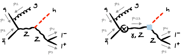
Figure 3: Example graphs that contribute to the B1g0Z matrix elements. The diagram on the left shows a SM contribution. On the right we instead depict a SMEFT correction that receives contributions from the generalised $hZZ$ and $h\gamma Z$ currents introduced in (13). The four-momentum flow is indicated by the grey arrows and labels. See the main text for additional explanations.

Insertions of the operators (2) and (3) lead to the Feynman diagrams shown on the right-hand side in Figure 1 at tree level. In order to capture this contribution in the case of the squared matrix element B1g0Z, one simply has to add the following term

$$\left(\frac{\delta g_{hZq}^{(1)\hskip 0.7113pth_{q}}\hskip 1.42262ptg_{Z\ell}^{h_{\ell}}}{D_{Z}(s_{45})}+\frac{g_{Zq}^{h_{q}}\hskip 2.13394pt\delta g_{hZ\ell}^{(1)\hskip 0.7113pth_{\ell}}}{D_{Z}(s_{123})}\right)\,{\cal A}_{\texttt{B1g0Z}}\left(1_{q}^{h_{q}},2_{g}^{h_{g}},3^{-h_{q}}_{\bar{q}};4_{\ell}^{h_{\ell}},5_{\bar{\ell}}^{-h_{\ell}}\right)\,,$$ (15)

to the corresponding dressed SM amplitude appearing within the modulus of (7). The analytic expressions for the couplings $\delta g_{hZf}^{(1)\hskip 0.7113pth_{f}}$ are given in Appendix A. In (15) the first term in the brackets describes the contribution from $Q_{Hq}^{(1)}$, $Q_{Hq}^{(3)}$, $Q_{Hd}$ and $Q_{Hu}$, while the second term is induced by $Q_{H\ell}^{(1)}$, $Q_{H\ell}^{(3)}$ and $Q_{He}$. Notice that compared to the corresponding SM contribution in (7) the SMEFT correction proportional to $\delta g_{hZq}^{(1)\hskip 0.7113pth_{q}}$ in (15) is missing the $Z$-boson propagator depending on $s_{123}$. This feature explains the high-energy growth Bishara:2020vix ; Bishara:2020pfx ; Bishara:2022vsc of the SMEFT $pp\to Vh$ amplitudes involving the Wilson coefficients $C_{Hq}^{(1)}$, $C_{Hq}^{(3)}$, $C_{Hd}$ and $C_{Hu}$.

The last type of SMEFT corrections to the squared matrix element B1g0Z is associated to the tree-level shifts of the SM parameters and couplings. EW input scheme corrections from $C_{HD}$, $C_{HW\!B}$, $C_{H\ell}^{(3)}$ and $C_{\ell\ell}$ lead to the shifts $\delta g_{1}$, $\delta g_{2}$ and $\delta v$ of the $U(1)_{Y}$ and $SU(2)_{L}$ gauge coupling and the Higgs vacuum expectation value (VEV), respectively, that in turn induce the shifts $\delta g_{hZZ}^{(0)}$ and $\delta g_{Zf}^{(0)\hskip 0.7113pth_{f}}$ in the respective couplings of the $Z$ boson. The expressions for these shifts are listed in Appendix A. In practice, the input scheme corrections can be accounted for by applying the replacements $g_{hZZ}\to g_{hZZ}+\delta g_{hZZ}^{(0)}$ and $g_{Zf}^{h_{f}}\to g_{Zf}^{h_{f}}+\delta g_{Zf}^{(0)\hskip 0.7113pth_{f}}$ to (7). Similarly, the Wilson coefficients $C_{Hq}^{(1)}$, $C_{Hq}^{(3)}$, $C_{Hd}$, $C_{Hu}$, $C_{H\ell}^{(1)}$, $C_{H\ell}^{(3)}$ and $C_{He}$ lead to direct shifts in the $Zf\bar{f}$ couplings that we include through the shifts $g^{h_{f}}_{Zf}\to g^{h_{f}}_{Zf}+\delta g^{(1)\hskip 0.7113pth_{f}}_{Zf}$ in (7). The expressions for the latter shifts are again given in Appendix A.

While we have used the spinor-helicity amplitudes ${\cal A}_{\texttt{B1g0Z}}$ in this section as examples to illustrate the general approach that we have employed in our SMEFT calculation of $pp\to Vh$ at NNLO in QCD, it is important to realise that the computation of all other spinor-helicity amplitudes and squared matrix elements proceeds in an analogous manner. In the case of the SMEFT corrections arising from the choice of EW input scheme as well as those associated to insertions of the operators (2) and (3) this is clear in view of the factorisation properties of these contributions $\big{(}$cf. (15)$\big{)}$. Likewise, since the spinor-helicity structure of the partonic part of a given SMEFT amplitude remains the same as in the SM, it can simply be extracted from the SM expressions and contracted with the part of the SMEFT amplitude that does change. It follows that an explicit calculation of the full partonic structures for the higher-order corrections to $pp\to Vh$ in the SMEFT can always be avoided, because the relevant amplitudes can be obtained from those in the SM by applying relations à la (11) and (14) which involves only spinor algebra. Still the calculation of all spinor contractions needed to achieve NNLO accuracy for the $pp\to Vh$ processes in the SMEFT is a non-trivial task and the final expressions for the spinor-helicity amplitudes turn out to be too lengthy to be reported here. All algebraic manipulations of spinor products needed in the context of this work have been performed with the aid of the Mathematica package S@M Maitre:2007jq .

3.3 Squared matrix element library

We provide all squared matrix elements discussed in the previous sections in a self-contained Fortran library GitLabAmplitudes . Our library includes the spinor-helicity amplitudes for the dimension-four SM and dimension-six SMEFT contributions as well as the definitions for the couplings and the propagators depending on the EW input scheme, which are combined and evaluated numerically in the squared matrix elements up to the desired SMEFT power counting order. Since several of these parts may be relevant in a broader context, we briefly outline the structure of the library. The file Bridge contains the general routines that are required to evaluate the squared matrix elements for a phase-space point, which is represented internally by an object of type Event_t. These routines allow to set up the numerical expressions for the spinor-helicity brackets, pass the input parameters to the Event_t object and calculate the dependent parameters for a chosen EW input scheme. The file squaredamps contains the squared matrix elements. The squared matrix element B1g0Z discussed above, for example, has the form B1g0Z(i1,i2,i3,i4,i5,K,f1,f2), where the integers $\texttt{i1},...,\texttt{i5}\in\{1,...,5\}$ allow to specify the crossing of the external legs, K is the Event_t object of the event, and f1 and f2 indicate the flavours of the quark and lepton lines present in the relevant topology, respectively. Our implementation employs the Monte Carlo Particle Numbering Scheme conventions of the PDG ParticleDataGroup:2022pth . The dimension-four, -six and -eight contributions to the squared matrix elements are calculated individually and their inclusion can be controlled via the flags SM, Linear and Quadratic of the Event_t object, respectively. Notice that the dimension-six or linear (dimension-eight or quadratic) SMEFT contributions arise from the interference of the SMEFT and SM amplitudes (self-interference of the SMEFT amplitudes). The spinor-helicity amplitudes, the loop coefficients and the functions implementing the parity and charge conjugation relations are collected in the amplib file. We point out that the required spinor-helicity amplitudes for $pp\to Z\to\ell^{+}\ell^{-}$ and $pp\to W\to\ell\nu$ production at NNLO in the SMEFT are just special cases of the amplitudes in our library. They can be obtained by setting up the Event_t object in the exact same way (for example giving it the four physical momenta of the external fermions in the case of B0g0Z), only that in this case the momenta will be linearly dependent because of momentum conservation.

Two further comments seem to be in order. First, besides including the squared matrix elements described above, we also provide the corresponding colour- and spin-correlated squared matrix elements that are required to build the infrared (IR) subtraction terms in the NNLO$+$PS implementation of $pp\to Vh$ production. In the case of B1g0V for instance the colour- and spin-correlated squared matrix elements are called B1g0V_colour and B1g0V_spin, respectively. The definition of these squared matrix elements follows the POWHEG conventions specified in (2.6) and (2.8) of the publication Alioli:2010xd . While the elements of B1g0V_colour are simply equal to B1g0V times colour factors, calculating B1g0V_spin requires a bit more care. In our notation, it takes the form

$$\begin{split}\texttt{B1g0Z\_spin}^{\mu\nu}&=\frac{8\pi\hskip 0.7113pt\alpha_{s}\hskip 0.7113ptC_{F}}{C_{A}}\sum_{h_{q},h_{\ell}=\pm}\left|\frac{g_{Zq}^{h_{q}}\hskip 1.42262ptg_{Z\ell}^{h_{\ell}}\hskip 1.42262ptg_{hZZ}}{D_{Z}(s_{123})\hskip 1.42262ptD_{Z}(s_{45})}\right|^{2}~{}\sum_{h_{g_{1}},h_{g_{2}}=\pm}\epsilon^{\mu\,\ast}_{h_{g_{1}}}\epsilon^{\nu}_{h_{g_{2}}}\,\\[5.69054pt] &\phantom{xx}\times{\cal A}_{\texttt{B1g0Z}}\left(1_{q}^{h_{q}},2_{g}^{h_{g_{1}}},3^{-h_{q}}_{\bar{q}};4_{\ell}^{h_{\ell}},5_{\bar{\ell}}^{-h_{\ell}}\right){\cal A}^{\dagger}_{\texttt{B1g0Z}}\left(1_{q}^{h_{q}},2_{g}^{h_{g_{2}}},3^{-h_{q}}_{\bar{q}};4_{\ell}^{h_{\ell}},5_{\bar{\ell}}^{-h_{\ell}}\right)\,,\end{split}$$ (16)

where the $\epsilon_{\pm}^{\mu}$ are polarisation vectors normalised as

$$\sum_{\mu,\nu}g_{\mu\nu}\,\epsilon_{h_{g_{1}}}^{\mu\,\ast}\epsilon_{h_{g_{2}}}^{\nu}=-\delta_{h_{g_{1}}h_{g_{2}}}\,,$$ (17)

with $g_{\mu\nu}=\text{diag}\left(1,-1,-1,-1\right)$. The polarisation vectors $\epsilon_{\pm}^{\mu}$ are implemented in POWHEG as

$$\epsilon^{\mu}_{[\texttt{PWG}]\pm}=\mp\frac{1}{\sqrt{2}}\left(\epsilon^{\mu}_{1}\pm i\epsilon^{\mu}_{2}\right)\,,$$ (18)

where the form of the four-vectors $\epsilon_{1}^{\mu}$ and $\epsilon_{2}^{\mu}$ can be found in (A.12) of Hagiwara:1988pp . In order to obtain $\mathcal{A}_{\texttt{B1g0Z}}$ as given in (5), we have however employed

$$\epsilon^{\mu}_{[\texttt{GHS}]+}=\frac{\left\langle 3|\gamma^{\mu}|2\right]}{\sqrt{2}\left\langle 32\right\rangle}\,,\qquad\epsilon^{\mu}_{[\texttt{GHS}]-}=\frac{\left\langle 2|\gamma^{\mu}|1\right]}{\sqrt{2}\left[21\right]}\,,$$ (19)

and therefore we have to take into account a complex phase

$$e^{i\varphi}\equiv\sum_{\mu,\nu}g_{\mu\nu}\,\epsilon^{\mu\ast}_{[\texttt{PWG}]+}\epsilon_{[\texttt{GHS}]-}^{\nu}\,.$$ (20)

See the discussion around (3.22) of Hasegawa:2009tx . We compute the phase $\varphi$ numerically and by taking it into account in our definition of the polarisation vectors allows us to compare our results for the squared matrix elements with previous implementations that are based on (18). Our implementation is further validated by the fact that the IR poles are properly cancelled in the POWHEG procedure.

Second, for the squared matrix element B1g1Z, we follow the discussion presented in the article Gehrmann:2011ab . There, the spinor-helicity amplitude is split into three primitive amplitudes $\mathcal{A}_{\Omega}$ with $\Omega=\alpha,\beta,\gamma$ and their corresponding loop coefficients $\Omega$:

$$\mathcal{A}_{\texttt{B1g1Z}}=\alpha\mathcal{A}_{\alpha}+\beta\mathcal{A}_{\beta}+\gamma\mathcal{A}_{\gamma}\,.$$ (21)

The loop coefficients $\Omega$ can be further divided into an IR divergent and an IR finite part as follows

$$\Omega=I^{(1)}(\epsilon)\,\Omega^{(0)}+\Omega^{(1),\,\text{finite}}\,,$$ (22)

with $I^{(1)}(\epsilon)$ the usual IR singularity operator as given for example in (C.9) of Gehrmann:2011ab . We include the $\mathcal{O}(1/\epsilon^{2})$, $\mathcal{O}(1/\epsilon)$ and $\mathcal{O}(1)$ pieces of $I^{(1)}(\epsilon)\,\Omega^{(0)}$ in the array entries $1$, $2$ and $3$ of the loop coefficients $\Omega$, respectively. Note that $\alpha^{(0)}=\beta^{(0)}=1$ and $\gamma^{(0)}=0$. The finite parts $\Omega^{(1),\,\text{finite}}$ are instead decomposed as

$$\Omega^{(1),\,\text{finite}}=C_{A}\,\Omega^{(1),\,\text{finite}}_{1}+\frac{1}{C_{A}}\,\Omega^{(1),\,\text{finite}}_{2}+\beta_{0}\,\Omega^{(1),\,\text{finite}}_{3}\,,$$ (23)

and include the leading colour, the subleading colour and the $\beta_{0}=(11\hskip 0.7113ptC_{A}-4\,T_{F}\hskip 0.35565ptN_{f})/6$ pieces individually. Here $T_{F}=1/2$ and $N_{f}=4$ denotes the number of active quark flavours. Analytic expressions for the coefficients $\Omega^{(1),\,\text{finite}}_{i}$ with $i=1,2,3$ were provided as FORM output in the arXiv submission of Gehrmann:2011ab for the three kinematical regions (i.e. $s_{13}>0$, $s_{12}>0$ and $s_{23}>0$) relevant at hadron colliders. They are expressed as one- and two-dimensional harmonic polylogarithms (HPLs) and we translate the appearing HPLs to logarithms and dilogarithms using the relevant formulae in Gehrmann:2000zt ; Gehrmann:2001jv , computing the latter numerically with the help of LoopTools Hahn:1998yk . The finite contributions $\Omega^{(1),\,\text{finite}}$ are added to the array entry 3 of the loop coefficients $\Omega$ in our code.

3.4 NNLO$+$PS implementation

In the following, we briefly describe how we consistently match the fixed-order NNLO SMEFT calculations of $pp\to Zh\to\ell^{+}\ell^{-}h$ and $pp\to Wh\to\ell\nu h$ production to a PS. We first recall that within the SM computations of the $pp\to Vh$ processes have recently reached NNLO$+$PS accuracy Astill:2018ivh ; Alioli:2019qzz ; Bizon:2019tfo ; Zanoli:2021iyp . In fact, here we follow the approach presented in Zanoli:2021iyp which employs the MiNNLO_PS method to match fixed-order QCD and PS effects. The interested reader is referred to the latter work and the articles Monni:2019whf ; Monni:2020nks for additional technical details not covered below.

In the case of Higgsstrahlung from ${\rm q\bar{q}F}$, the starting point of our NNLO$+$PS implementation is the computation of the $q\bar{q}\to Vh$ channel in association with one light QCD parton at NLO according to the POWHEG method Nason:2004rx ; Frixione:2007vw , inclusive in the radiation of a second light QCD parton. The computation of the relevant matrix elements has been outlined in Section 3.1 and relies on the SM spinor-helicity amplitudes calculated in Kramer:1986sg ; Hamberg:1990np ; Gehrmann:2011ab ; Majer:2020kdg . In a second step, an appropriate Sudakov form factor and higher-order corrections are applied such that the calculation remains finite in the unresolved limit of the light partons and NNLO accurate for inclusive $q\bar{q}\to Vh$ production. In the third step, the kinematics of the second radiated parton (accounted for inclusively in the first step) is generated following the POWHEG method to preserve the NLO accuracy of the $Vh$ plus jet cross section, including subsequent radiation through Pythia 8.2 Sjostrand:2014zea . We stress that since all emissions are ordered in transverse momentum ($p_{T}$) and the used Sudakov form factor matches the leading logarithms generated by Pythia 8.2, the MiNNLO_PS approach maintains the leading-logarithmic accuracy of the PS. The ggF one-loop contributions to Higgsstrahlung, i.e. the $gg\to Zh$ process, can instead be computed independently at LO$+$PS and simply added to the ${\rm q\bar{q}F}$ results. Following the general discussion in Section 3.2 the relevant SMEFT spinor-helicity amplitudes can be obtained from those in the SM. We take the SM amplitudes from the MCFM implementation Boughezal:2016wmq of the results obtained in Campbell:2016jau . Further details on our implementation of the $gg\to Zh$ process are given in Appendix B.

Our MiNNLO_PS generator for $q\bar{q}\to Vh$ production has been implemented into the POWHEG-BOX. While it uses the infrastructure of the NNLO$+$PS SM Higgsstrahlungs generator Zanoli:2021iyp the parts of the code that calculate the squared matrix elements are entirely new and independent. To validate our implementation of the SM computation we have performed extensive numerical checks against Zanoli:2021iyp . The individual spinor-helicity amplitudes were furthermore compared to a private implementation of the results presented in Majer:2020kdg (which entered the calculation Gauld:2019yng ), and results for the squared matrix elements were numerically validated with OpenLoops 2 Buccioni:2019sur . We exploit the Frixione-Kunszt-Signer subtraction Frixione:1995ms ; Frixione:1997np to deal with soft and collinear singularities of the real contributions and to cancel the IR poles of the virtual corrections. In fact, the full POWHEG-BOX machinery is used that automatically builds the soft and collinear counterterms and remnants, and also verifies the behaviour in the soft and collinear limits of the real squared matrix elements against their soft and collinear approximations. These checks provide non-trivial tests of our SMEFT calculation of Higgsstrahlung in the ${\rm q\bar{q}F}$ channel. In the case of the $gg\to Zh$ channel we have instead written a simple LO$+$PS generator using the POWHEG-BOX framework. Our implementation of the corresponding SM spinor-helicity amplitudes has been validated numerically against OpenLoops 2 at the level of the squared matrix elements.

Besides the direct SMEFT contributions described in Section 3.2 the $pp\to Vh$ processes also receive corrections from the propagators of the $Z$ and $W$ boson, because SMEFT operators generically modify the masses and the total decay widths of all unstable particles. Our POWHEG-BOX implementation contains the complete tree-level shifts of the relevant masses and total decay widths that are induced by the Wilson coefficients of the operators (1) to (4) for the $\alpha$, the $\alpha_{\mu}$ as well as the LEP scheme — cf. Appendix A for a comprehensive discussion of the different EW input schemes in the SMEFT. For instance, in the case of the total decay width of the $Z$ and $W$ boson in the LEP scheme we find the relevant shifts

$$\begin{split}\delta\Gamma_{Z}&\simeq-\frac{v^{2}}{\Lambda^{2}}\,\Big{[}\,1.99\hskip 0.7113ptC_{HW\!B}-1.14\hskip 0.7113ptC_{Hq}^{(1)}-3.89\hskip 0.7113ptC_{Hq}^{(3)}+0.46\hskip 0.7113ptC_{Hd}-0.62\hskip 0.7113ptC_{Hu}\\[2.84526pt] &\hskip 39.83368pt+0.46\hskip 0.7113ptC_{H\ell}^{(1)}+4.98\hskip 0.7113ptC_{H\ell}^{(3)}+0.46\hskip 0.7113ptC_{He}+1.63\hskip 0.7113ptC_{HD}-3.25\hskip 0.7113ptC_{\ell\ell}\,\Big{]}\,{\rm GeV}\,,\\[5.69054pt] \delta\Gamma_{W}&\simeq-\frac{v^{2}}{\Lambda^{2}}\,\Big{[}\,4.77\hskip 0.7113ptC_{HW\!B}-2.67\hskip 0.7113ptC_{Hq}^{(3)}+5.31\hskip 0.7113ptC_{H\ell}^{(3)}+2.16\hskip 0.7113ptC_{HD}-3.32\hskip 0.7113ptC_{\ell\ell}\,\Big{]}\,{\rm GeV}\,.\end{split}$$ (24)

These results agree with those presented in the literature $\big{(}$cf. for instance Dawson:2019clf $\big{)}$. We stress that we do not perform an expansion in the SMEFT corrections to the propagators of the $Z$ and $W$ boson. In consequence, the dependence on the Wilson coefficients of our numerical results is generally non-linear. The resulting non-linear effects are however always very small.

4 Anatomy of SMEFT effects

In this section, we motivate simple SMEFT benchmark scenarios by discussing the leading experimental constraints on the Wilson coefficients of the dimension-six operators introduced in (1) to (4). In this discussion the choice of an EW input scheme is an important ingredient. While in our POWHEG-BOX implementation the user can choose between the $\alpha$, $\alpha_{\mu}$, and LEP schemes (see Appendix A for a brief discussion of EW input schemes in the SMEFT) the following discussion is based on the LEP scheme which uses as inputs $\{\alpha,G_{F},m_{Z}\}$. Here $\alpha$ is the fine-structure constant, $G_{F}$ is the Fermi constant as extracted from muon decay and $m_{Z}$ is the mass of the $Z$ boson in the on-shell scheme.

In the LEP scheme, the weak mixing angle $\theta_{w}$, the $U(1)_{Y}$ and $SU(2)_{L}$ couplings $g_{1}$ and $g_{2}$ and the VEV of the Higgs boson $v$ can all be written in terms of the EW input parameters $\{\alpha,G_{F},m_{Z}\}$. One finds the following relations

$$s_{w}^{2}=\frac{1}{2}\left[1-\sqrt{1-\frac{2\sqrt{2}\pi\alpha}{G_{F}\hskip 0.35565ptm_{Z}^{2}}}\right]\simeq 0.23\,,$$ (25)

and

$$g_{1}=\frac{\sqrt{4\pi\alpha}}{c_{w}}\simeq 0.36\,,\qquad g_{2}=\frac{\sqrt{4\pi\alpha}}{s_{w}}\simeq 0.65\,,\qquad v=\frac{1}{\sqrt[4]{2}\hskip 0.7113pt\sqrt{G_{F}}}\simeq 246.22\,{\rm GeV}\,,$$ (26)

where the given numerical values correspond to $\alpha=1/127.951$, $G_{F}=1.1663788\cdot 10^{-5}\,{\rm GeV}^{-2}$ and $m_{Z}=91.1876\,{\rm GeV}$ ParticleDataGroup:2022pth . Notice that in (25) and (26) we have used the abbreviations $s_{w}$ and $c_{w}$ to denote the sine and cosine of the weak mixing angle, respectively.

4.1 $W$-boson mass

The on-shell mass of the $W$ boson is a predicted quantity in the LEP scheme as well. In terms of the results (25) and (26) one has

$$m_{W}=c_{w}\hskip 0.7113ptm_{Z}\simeq 79.83\,{\rm GeV}\,.$$ (27)

The corresponding relative tree-level shift of $m_{W}$ induced in the $U(3)^{5}$ symmetric SMEFT is given by

$$\begin{split}\frac{\delta m_{W}}{m_{W}}&=-\frac{c_{w}\hskip 0.7113pts_{w}}{2\left(c_{w}^{2}-s_{w}^{2}\right)}\frac{v^{2}}{\Lambda^{2}}\left[2\hskip 0.7113ptC_{HW\!B}+\frac{s_{w}}{c_{w}}\left(2\hskip 0.7113ptC_{H\ell}^{(3)}-C_{\ell\ell}\right)+\frac{c_{w}}{2\hskip 0.7113pts_{w}}\,C_{HD}\right]\\[5.69054pt] &\simeq-0.048\hskip 1.42262ptC_{HW\!B}-0.027\hskip 0.7113ptC_{H\ell}^{(3)}-0.022\hskip 0.7113ptC_{HD}+0.013\hskip 0.7113ptC_{\ell\ell}\,,\end{split}$$ (28)

where we have employed (25), (26) and assumed $\Lambda=1\,{\rm TeV}$ for the energy scale that suppresses the dimension-six operators to obtain the numerical results presented in the second line. Employing the latest world average of the measured $W$-boson mass obtained by the PDG ParticleDataGroup:2022pth and the state-of-the-art SM prediction Chen:2020xot , we obtain the following 95% confidence level (CL) limit

$$\frac{\delta m_{W}}{m_{W}}\in[-0.9,5.6]\cdot 10^{-4}\,,$$ (29)

on the allowed relative shift of $m_{W}$. This result in general sets stringent constraints on the Wilson coefficients entering (28). For instance, in the case of the operator $Q_{HW\!B}$ we find the bound

$$\frac{C_{HW\!B}}{\Lambda^{2}}\in[-1.2,0.2]\cdot 10^{-2}\,{\rm TeV}^{-2}\,,$$ (30)

if all other Wilson coefficients in (28) are set to zero. Similar though weaker limits also apply in the case of $C_{HD}$, $C_{H\ell}^{(3)}$ and $C_{\ell\ell}$ if each of the Wilson coefficients is treated as the only non-zero contribution.

4.2 $Z$-boson couplings

The linear combinations of Wilson coefficients that modify the couplings of the $W$ and $Z$ boson to fermions at tree level are strongly constrained by the EW precision measurements performed at LEP and SLD. In the case of the $Z$ boson the shifts of the left- and right-handed couplings to a fermion $\psi=\{e,\nu,d,u\}$ take the following form

$$\begin{split}\delta g_{L}^{\psi}&=\frac{g_{2}}{c_{w}}\,\frac{v^{2}}{\Lambda^{2}}\left[g_{T^{3}_{\psi}}\hskip 0.7113ptT^{3}_{\psi}-g_{Q_{\psi}}\hskip 0.7113ptQ_{\psi}-\frac{1}{2}\left(C_{H\psi_{L}}^{(1)}-2\hskip 0.7113ptT_{\psi}^{3}\hskip 0.7113ptC_{H\psi_{L}}^{(3)}\right)\right]\,,\\[5.69054pt] \delta g_{R}^{\psi}&=\frac{g_{2}}{c_{w}}\,\frac{v^{2}}{\Lambda^{2}}\left[-g_{Q_{\psi}}\hskip 0.7113ptQ_{\psi}-\frac{1}{2}\left(1-\delta_{\psi\nu}\right)C_{H\psi_{R}}\right]\,,\end{split}$$ (31)

with

$$g_{T^{3}_{\psi}}=-C_{H\ell}^{(3)}-\frac{C_{HD}}{4}+\frac{C_{\ell\ell}}{2}\,,\qquad g_{Q_{\psi}}=\frac{c_{w}\hskip 0.7113pts_{w}}{c_{w}^{2}-s_{w}^{2}}\left[C_{HW\!B}-\frac{s_{w}}{c_{w}}\,g_{T^{3}_{\psi}}\right]\,.$$ (32)

Here the coupling $g_{2}$ is defined via (26), $\psi_{L}=\{\ell,q\}$ and $\psi_{R}=\{e,d,u\}$, while $T^{3}_{\psi}=\pm 1/2$ denotes the weak isospin eigenvalue, $Q_{\psi}$ is the electric charge of the fermion $\psi$ in units of $e=\sqrt{4\pi\alpha}$. Notice that the expressions given in (32) correspond to the LEP scheme and that we have assumed that the Wilson coefficients of the operators that involve fermionic fields are flavour universal. Below we will assume that such a flavour universality holds for all SM fermions apart from the charm, bottom and top quark.

In the case of the electron the formulae (31) and (32) lead to the following left- and right-handed coupling shifts

$$\begin{split}\delta g_{L}^{e}&\simeq 0.036\hskip 1.42262ptC_{HW\!B}-0.022\hskip 0.7113ptC_{H\ell}^{(1)}+0.020\hskip 0.7113ptC_{H\ell}^{(3)}+0.011\hskip 0.7113ptC_{HD}-0.021\hskip 0.7113ptC_{\ell\ell}\,,\\[5.69054pt] \delta g_{R}^{e}&\simeq 0.036\hskip 1.42262ptC_{HW\!B}+0.020\hskip 0.7113ptC_{H\ell}^{(3)}-0.022\hskip 0.7113ptC_{He}+0.005\hskip 0.7113ptC_{HD}-0.010\hskip 0.7113ptC_{\ell\ell}\,,\end{split}$$ (33)

when (25), (26) and $\Lambda=1\,{\rm TeV}$ are used as numerical inputs. The EW precision measurements performed by LEP and SLD ALEPH:2005ab ; ParticleDataGroup:2022pth imply that at 95% CL one has

$$\delta g_{L}^{e}\in[-7.1,2.0]\cdot 10^{-4}\,,\qquad\delta g_{R}^{e}\in[-7.0,1.6]\cdot 10^{-4}\,.$$ (34)

Ignoring cancellations these limits again put severe constraints on the Wilson coefficients that appear in (33). Numerically, we obtain for instance the bounds

$$\frac{C_{H\ell}^{(3)}}{\Lambda^{2}}\in[-3.6,1.0]\cdot 10^{-2}\,{\rm TeV}^{-2}\,,\qquad\frac{C_{He}}{\Lambda^{2}}\in[-0.7,3.1]\cdot 10^{-2}\,{\rm TeV}^{-2}\,,$$ (35)

from the constraint on $\delta g_{L}^{e}$ and $\delta g_{R}^{e}$, respectively, if we allow only the considered Wilson coefficient to take a non-vanishing value. We add that the Wilson coefficients $C_{HD}$, $C_{H\ell}^{(1)}$ and $C_{\ell\ell}$ can also be constrained by the LEP and SLD measurements of the $Z$-boson coupling to neutrinos. The obtained bounds, however, turn out to be weaker than those that derive from (33) and (34).

Employing again (25), (26), (31) and (32) the left- and right-handed coupling shifts in the case of the down and up quark take the following form

$$\begin{split}\delta g_{L}^{d}&\simeq 0.012\hskip 1.42262ptC_{HW\!B}-0.022\left(C_{Hq}^{(1)}+C_{Hq}^{(3)}\right)+0.029\hskip 0.7113ptC_{H\ell}^{(3)}+0.007\hskip 0.7113ptC_{HD}-0.015\hskip 0.7113ptC_{\ell\ell}\,,\\[5.69054pt] \delta g_{R}^{d}&\simeq 0.012\hskip 1.42262ptC_{HW\!B}-0.022\hskip 0.7113ptC_{Hd}+0.007\hskip 0.7113ptC_{H\ell}^{(3)}+0.002\hskip 0.7113ptC_{HD}-0.003\hskip 0.7113ptC_{\ell\ell}\,,\\[5.69054pt] \delta g_{L}^{u}&\simeq-0.024\hskip 1.42262ptC_{HW\!B}-0.022\left(C_{Hq}^{(1)}-C_{Hq}^{(3)}\right)-0.036\hskip 0.7113ptC_{H\ell}^{(3)}-0.009\hskip 0.7113ptC_{HD}+0.018\hskip 0.7113ptC_{\ell\ell}\,,\\[5.69054pt] \delta g_{R}^{u}&\simeq-0.024\hskip 1.42262ptC_{HW\!B}-0.022\hskip 0.7113ptC_{Hu}-0.013\hskip 0.7113ptC_{H\ell}^{(3)}-0.003\hskip 0.7113ptC_{HD}+0.007\hskip 0.7113ptC_{\ell\ell}\,,\end{split}$$ (36)

for a common operator suppression scale of $\Lambda=1\,{\rm TeV}$. The measurements by LEP and SLD performed at the $Z$-pole lead to the following limits

$$\begin{split}&\delta g_{L}^{d}\in[-6.2,2.0]\cdot 10^{-2}\,,\qquad\delta g_{R}^{d}\in[-4.8,3.4]\cdot 10^{-2}\,,\\[5.69054pt] &\hskip 2.84526pt\delta g_{L}^{u}\in[0.2,6.8]\cdot 10^{-2}\,,\qquad\delta g_{R}^{u}\in[-1.3,5.3]\cdot 10^{-2}\,,\end{split}$$ (37)

at 95% CL. These bounds translate into

$$\begin{split}&\frac{C_{Hq}^{(1)}}{\Lambda^{2}}\in[-0.9,2.8]\;{\rm TeV}^{-2}\,,\qquad\frac{C_{Hq}^{(3)}}{\Lambda^{2}}\in[-0.9,2.8]\;{\rm TeV}^{-2}\,,\\[5.69054pt] &\frac{C_{Hd}}{\Lambda^{2}}\in[-1.5,2.1]\;{\rm TeV}^{-2}\,,\qquad\frac{C_{Hu}}{\Lambda^{2}}\in[-2.4,0.6]\;{\rm TeV}^{-2}\,,\end{split}$$ (38)

if each Wilson coefficient is treated independently and the limit on $\delta g_{L}^{d}$ as given in (37) is used to constrain $C_{Hq}^{(1)}$ and $C_{Hq}^{(3)}$. We emphasise that notably more stringent limits on the Wilson coefficients in (38) would be obtained if one were to perform a complete EW fit including heavy flavour measurements and assume a SMEFT Lagrangian with an approximate $U(3)^{5}$ symmetry. This is a simple consequence of the fact that in such a case one has $\delta g_{L,R}^{b}=\delta g_{L,R}^{d}$ ($\delta g_{L,R}^{c}=\delta g_{L,R}^{u}$) and that the bottom (charm) couplings were significantly better determined than the down (up) couplings at LEP and SLD — see for example Figure F.3 in ALEPH:2005ab . The limits (38) are relaxed because they assume flavour universality only for the down and strange quark as far as quarks are concerned.

4.3 Higgs-boson observables

The Wilson coefficients of the operators (1) modify the Higgs signal strengths in final states with two vector bosons. In the LEP scheme and including only the tree-level SMEFT corrections due to $C_{HB}$, $C_{HW}$ and $C_{HW\!B}$ the coupling modifiers relevant for $h\to WW$ and $h\to ZZ$ can be written in the $\kappa$ framework as follows Falkowski:2019hvp

$$\begin{split}\delta\kappa_{WW}&\simeq-\frac{v^{2}}{\Lambda^{2}}\,\Big{[}0.76\hskip 0.7113ptC_{HW}+3.18\hskip 0.7113ptC_{HW\!B}\Big{]}\,,\\[5.69054pt] \delta\kappa_{ZZ}&\simeq\frac{v^{2}}{\Lambda^{2}}\,\Big{[}2.71\hskip 0.7113ptC_{HB}-3.18\hskip 0.7113ptC_{HW}+1.23\hskip 0.7113ptC_{HW\!B}\Big{]}\,.\end{split}$$ (39)

In the tree-level approximation the corresponding expressions for the $h\to\gamma\gamma$ and $h\to\gamma Z$ decays do not depend on the choice of the EW input scheme. One finds

$$\begin{split}\delta\kappa_{\gamma\gamma}&\simeq\frac{1}{g_{h\gamma\gamma}}\frac{v^{2}}{\Lambda^{2}}\,\Big{[}c_{w}^{2}\hskip 0.7113ptC_{HB}+s_{w}^{2}\hskip 0.7113ptC_{HW}-c_{w}\hskip 0.7113pts_{w}\hskip 0.7113ptC_{HW\!B}\Big{]}\,,\\[5.69054pt] \delta\kappa_{\gamma Z}&\simeq-\frac{1}{g_{h\gamma Z}}\frac{v^{2}}{\Lambda^{2}}\,\Big{[}2\hskip 0.7113ptc_{w}\hskip 0.7113pts_{w}\left(C_{HB}-C_{HW}\right)+\left(c_{w}^{2}-s_{w}^{2}\right)C_{HW\!B}\Big{]}\,,\end{split}$$ (40)

where $g_{h\gamma\gamma}\simeq-2.02\cdot 10^{-3}$ and $g_{h\gamma Z}\simeq-7.23\cdot 10^{-3}$ parameterise the loop-induced $h\gamma\gamma$ and $h\gamma Z$ couplings within the SM. Explicit analytic formulae for $g_{h\gamma\gamma}$ and $g_{h\gamma Z}$ can be found for instance in Brivio:2020onw .

Assuming that the ggF Higgs production cross section is SM-like and taking the SM predictions for the total decay width of the Higgs and its branching ratios from LHCHiggsWG4 , we obtain for $\Lambda=1\,{\rm TeV}$ the following linearised expressions for the relevant signal strenghts

$$\begin{split}&\mu_{\rm ggF}^{WW}\simeq 1+0.074\hskip 0.7113ptC_{HB}-0.0086\hskip 0.7113ptC_{HW}\,,\qquad\mu_{\rm ggF}^{ZZ}\simeq 1+0.40\hskip 0.7113ptC_{HB}-0.30\hskip 0.7113ptC_{HW}\,,\\[5.69054pt] &\hskip 11.38109pt\mu_{\rm ggF}^{\gamma\gamma}\simeq 1-46.0\hskip 0.7113ptC_{HB}-14.0\hskip 0.7113ptC_{HW}\,,\qquad\mu_{\rm ggF}^{\gamma Z}\simeq 1+14.3\hskip 0.7113ptC_{HB}-14.1\hskip 0.7113ptC_{HW}\,.\end{split}$$ (41)

Notice that in view of (30) we have neglected the contributions of the Wilson coefficient $C_{HW\!B}$ in (41). The corresponding measured Higgs signal strenghts are

$$\mu_{\rm ggF}^{WW}=1.18\pm 0.13\,,\quad\mu_{\rm ggF}^{ZZ}=0.96\pm 0.08\,,\quad\mu_{\rm ggF}^{\gamma\gamma}=1.05\pm 0.09\,,\quad\mu_{\rm ggF}^{\gamma Z}=2.2\pm 0.7\,.$$ (42)

Here the first three results represent unofficial weighted averages of the ATLAS ATLAS:2020qdt and CMS CMS:2020gsy measurements, while the fourth result stems from an official combination performed by the ATLAS and CMS collaborations in CMS:2023mku .

By comparing (41) and (42) it is evident that under the assumption of $C_{HW\!B}\simeq 0$ the constraints on the Wilson coefficients $C_{HB}$ and $C_{HW}$ from $h\to\gamma\gamma$ and $h\to\gamma Z$ are in general more stringent than those that arise from $h\to WW$ and $h\to ZZ$. In fact, since the signal strength $\mu_{\rm ggF}^{\gamma\gamma}$ is at present significantly better measured than $\mu_{\rm ggF}^{\gamma Z}$, all combinations of Wilson coefficients that obey

$$C_{HB}\simeq-\frac{s_{w}^{2}}{c_{w}^{2}}\,C_{HW}\simeq-0.30\hskip 1.42262ptC_{HW}\,,$$ (43)

are most weakly constrained by (42). Notice that for Wilson coefficients $C_{HB}$ and $C_{WB}$ satisfying (43) and $|C_{HW}|$ sufficiently small the signal strengths $\mu_{\rm ggF}^{WW}$, $\mu_{\rm ggF}^{ZZ}$ and $\mu_{\rm ggF}^{\gamma\gamma}$ are all predicted to be SM-like, while $\mu_{\rm ggF}^{\gamma Z}$ can at the same time be notably different from one.

4.4 Discussion

We are now in a position to identify simple benchmark scenarios for the full set of Wilson coefficients of the operators defined in (1) to (4). As a common operator suppression scale we hereafter take $\Lambda=1\,{\rm TeV}$. In view of the stringent constraints arising from (28), (29), (33) and (34) we always employ

$$C_{H\ell}^{(1)}=C_{H\ell}^{(3)}=C_{He}=C_{H\Box}=C_{HD}=C_{\ell\ell}=0\,,$$ (44)

when studying the numerical impact of the SMEFT dimension-six operators (1) to (4) on $Zh$ production at the LHC in Section 5.

In the case of the dimension-six operators that modify the couplings between the Higgs and two vector bosons at tree level, we choose the following values for the Wilson coefficients

$$C_{HB}=0.015\,,\qquad C_{HW}=-0.05\,,\qquad C_{HW\!B}=0\,,$$ (45)

where the choice of $C_{HW\!B}$ is motivated by (30). The values (45) lead to the following Higgs signal strengths

$$\mu_{\rm ggF}^{WW}\simeq 1.00\,,\qquad\mu_{\rm ggF}^{ZZ}\simeq 1.02\,,\qquad\mu_{\rm ggF}^{\gamma\gamma}\simeq 1.01\,,\qquad\mu_{\rm ggF}^{\gamma Z}\simeq 2.13\,,$$ (46)

if one assumes that the ggF Higgs production cross section in the SMEFT is equal to that of the SM and sets to zero the Wilson coefficients of all the operators appearing in (2) to (4). Notice that the predictions (46) are all SM-like apart from $\mu_{\rm ggF}^{\gamma Z}$ which is close to the central value of the measured signal strength given in (42). When considering the benchmark scenario (45) we will, besides employing (44), also set all the Wilson coefficients of the operators (2) to zero.

In the case of the operators that result in couplings between the Higgs, a $W$ or a $Z$ boson, and light quarks, we consider the four benchmark scenarios

$$C_{Hq}^{(3)}=0.05\,,\qquad C_{Hq}^{(1)}=C_{Hd}=C_{Hu}=0\,,$$ (47)

$$\!C_{Hd}=-0.1\,,\qquad C_{Hq}^{(1)}=C_{Hq}^{(3)}=C_{Hu}=0\,,$$ (48)

$$\,C_{Hu}=0.1\,,\qquad C_{Hq}^{(1)}=C_{Hq}^{(3)}=C_{Hd}=0\,,$$ (49)

$$C_{Hq}^{(1)}=0.05\,,\qquad C_{Hq}^{(3)}=C_{Hd}=C_{Hu}=0\,,$$ (50)

where one of the four relevant Wilson coefficients is non-zero while the remaining ones vanish identically. As in the case of (45) we set all Wilson coefficients not present in (47) to (50) to zero when considering the class of operators introduced in (2).

5 Phenomenological analysis

In the following, we present NNLO$+$PS accurate results for $pp\to Zh\to\ell^{+}\ell^{-}h$ production with a stable Higgs boson including the SMEFT effects discussed in Section 3. All SM input parameters are taken from the most recent PDG review ParticleDataGroup:2022pth . In particular, we use $\alpha=1/127.951$, $G_{F}=1.1663788\cdot 10^{-5}\,{\rm GeV}^{-2}$, $m_{Z}=91.1876\,{\rm GeV}$, $\Gamma_{Z}^{\rm SM}=2.4952\,{\rm GeV}$, $m_{h}=125.09\,{\rm GeV}$ and $\Gamma_{h}^{\rm SM}=4.1\,{\rm MeV}$. The values of the weak mixing angle, the $U(1)_{Y}$ and $SU(2)_{L}$ gauge coupling and the Higgs VEV are calculated from (25) and (26), respectively, meaning that we work in the LEP scheme. The NNPDF31_nnlo_as_01180 parton distribution functions (PDFs) NNPDF:2017mvq are employed in our MC simulations and events are showered with Pythia 8.2 Sjostrand:2014zea utilising the Monash tune Skands:2014pea . To target the $Z\to\ell^{+}\ell^{-}$ decay, we select events with two charged leptons (electrons or muons). The leptons are defined at the dressed level, meaning the lepton four-momentum is combined with the four-momenta of nearby prompt photons arising in the shower using a dressing-cone size of $\Delta R_{\ell\gamma}<0.1$. The leptons are required to have $p_{T,\ell}>15\,{\rm GeV}$ and a pseudorapidity of $|\eta_{\ell}|<2.5$. The invariant mass of the dilepton pair is restricted to $m_{\ell^{+}\ell^{-}}\in[75,105]\,{\rm GeV}$. These restrictions are close to those imposed by the existing ATLAS and CMS studies of ATLAS:2018kot ; CMS:2018nsn ; ATLAS:2019yhn ; ATLAS:2020fcp ; CMS:2022exo and we will simply refer to them as “fiducial cuts” in what follows.

The four panels in Figure LABEL:fig:bench1 display our NNLO$+$PS predictions for $pp\to Zh\to\ell^{+}\ell^{-}h$ in the SMEFT benchmark scenario (45) assuming $\Lambda=1\,{\rm TeV}$ and LHC collisions with a centre-of-mass energy of $\sqrt{s}=13\,{\rm TeV}$. The fiducial cross sections differential in the $Z$-boson pseudorapidity $|\eta_{Z}|$ (upper left) and transverse momentum $p_{T,Z}$ (upper right) as well as the pseudorapidity difference $|\eta_{Z}-\eta_{h}|$ (lower left) and the invariant mass $m_{Zh}$ (lower right) of the $Zh$ system are shown. The central renormalisation scale $\mu_{R}$ and factorisation scale $\mu_{F}$ are set according to the MiNNLO_PS procedure Monni:2019whf ; Monni:2020nks and the grey bands in the lower panels represent the corresponding perturbative uncertainties in the SM. These uncertainties have been obtained from seven-point scale variations enforcing the constraint $1/2\leq\mu_{R}/\mu_{F}\leq 2$. Within the SM they do not exceed $5\%$ for what concerns the considered distributions, and relative scale uncertainties of very similar size are also found in the case of the SMEFT spectra. The SM predictions are indicated by the solid black lines while the solid (dotted) orange curves represent the SMEFT contributions that are linear (quadratic) in the Wilson coefficients. Notice that the linear (quadratic) SMEFT contributions arise from the interference of the SMEFT and SM amplitudes (self-interference of the SMEFT amplitudes). The solid dark orange lines finally correspond to the sums of the linear and quadratic SMEFT contributions. We observe that in the case of the $|\eta_{Z}|$ distribution the SMEFT effects related to $C_{HB}$ and $C_{HW}$ to first approximation simply shift the spectra by a constant amount. In the cases of the $p_{T,Z}$, the $|\eta_{Z}-\eta_{h}|$ and the $m_{Zh}$ spectra the relative sizes of the SMEFT corrections instead grow with increasing $p_{T,Z}$, $|\eta_{Z}-\eta_{h}|$ and $m_{Zh}$, respectively. It is also evident from all panels that the quadratic SMEFT contributions are negligibly small compared to the linear terms. Numerically, we find that the benchmark scenario (45) leads to relative corrections of around $+2\%$ to $+5\%$ in the studied distributions — the fiducial cross section is enhanced by $+3.5\%$ compared to the SM. Notice that while the predicted deviations are sometimes larger than the corresponding SM scale uncertainties, they are typically smaller than the ultimate projected HL-LHC accuracy in $Zh$ production channel that amounts to $5\%$ ATLAS:2018jlh ; CMS:2018qgz . From this numerical exercise one can conclude that future constraints on the Wilson coefficients $C_{HB}$, $C_{HW}$ and $C_{HW\!B}$ from $Vh$ production are unlikely to be as stringent as the limits that future determinations of the Higgs signal strengths in $h\to\gamma\gamma$ and $h\to\gamma Z$ will allow to set. This will in particular be the case if both Higgs signal strengths turn out to be SM-like $\big{(}$see (41) and (42)$\big{)}$.

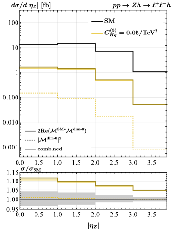
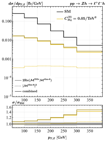
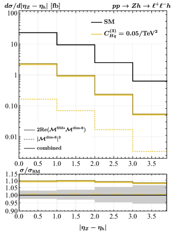
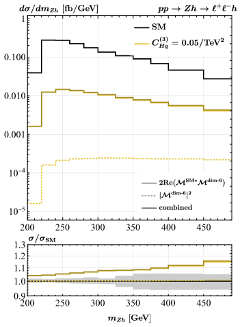
Figure 4: As Figure LABEL:fig:bench1 but for benchmark scenario (47) with $\Lambda=1\,{\rm TeV}$. The yellow lines correspond to the BSM results.

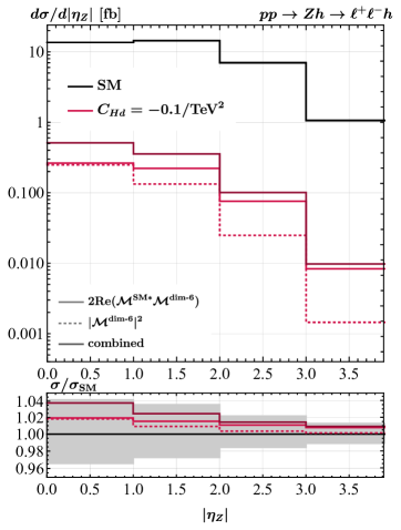
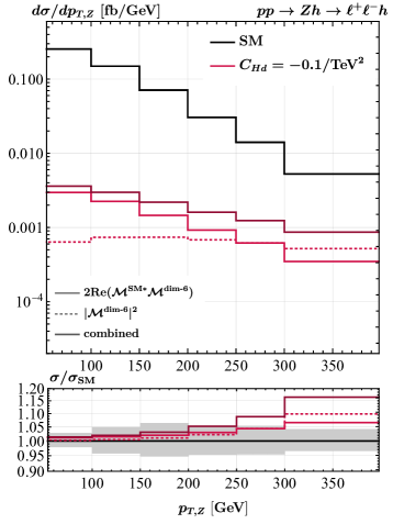
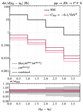
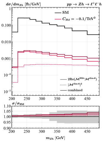
Figure 5: As Figure LABEL:fig:bench1 but for benchmark scenario (48) assuming $\Lambda=1\,{\rm TeV}$. The red curves represent the BSM results.

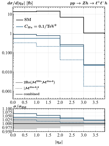
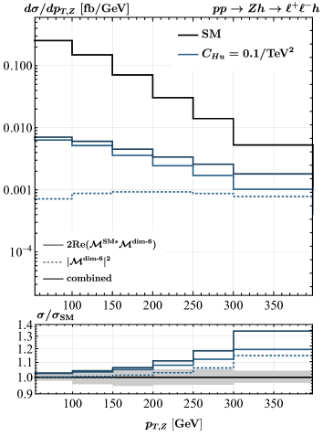
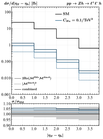
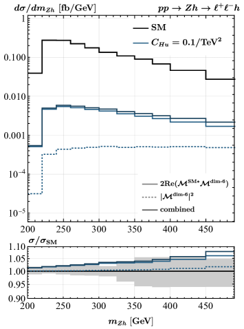
Figure 6: As Figure LABEL:fig:bench1 but for benchmark scenario (49) with $\Lambda=1\,{\rm TeV}$. The blue lines are the BSM results.

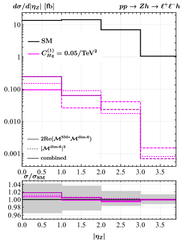
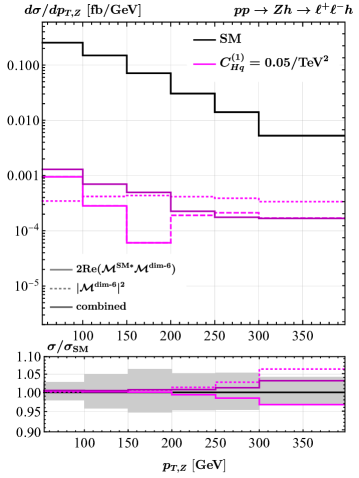
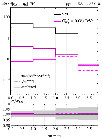
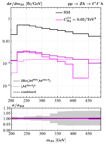
Figure 7: As Figure LABEL:fig:bench1 but for benchmark scenario (50) assuming $\Lambda=1\,{\rm TeV}$. The SMEFT predictions are coloured in magenta. In the case of the linear SMEFT contributions the solid (dashed) lines correspond to positive (negative) corrections to the relevant distribution.

Figures 4 to 6 contain our NNLO$+$PS predictions for $pp\to Zh\to\ell^{+}\ell^{-}h$ production in the SMEFT benchmark scenarios (47) to (49). In all cases we have employed an operator suppression scale of $\Lambda=1\,{\rm TeV}$. The results depicted in the first three figures show very similar features. In all cases the relative SMEFT corrections are rather flat in the $|\eta_{Z}|$ and $|\eta_{Z}-\eta_{h}|$ distributions, while in the case of the $p_{T,Z}$ and $m_{Zh}$ spectra they get larger with increasing $p_{T,Z}$ and $m_{Zh}$. The observed high-energy growth is expected from (15) and in all three cases most pronounced in the $p_{T,Z}$ distribution. One also sees that the linear SMEFT effects are largest in the benchmark scenario with $C_{Hq}^{(3)}=0.05$ where they can exceed $+50\%$ compared to the SM for $p_{T,Z}>300\,{\rm GeV}$. The respective effects in the benchmark scenario with $C_{Hd}=-0.1$ ($C_{Hu}=0.1$) just correspond to around $+7\%$ ($+20\%$). The observed hierarchy of SMEFT effects can be traced back to the approximate pattern $g_{L}^{d,{\rm SM}}\simeq-g_{L}^{u,{\rm SM}}\simeq-6\hskip 0.7113ptg_{R}^{d,{\rm SM}}\simeq 3\hskip 0.7113ptg_{R}^{u,{\rm SM}}$ of left- and right-handed $Z$-boson couplings within the SM and the feature $\delta g_{L}^{d}\propto-C_{Hq}^{(3)}$ and $\delta g_{L}^{u}\propto C_{Hq}^{(3)}$ — see (36). Notice also that the size of the quadratic SMEFT corrections is relatively small in the case of (47) while these effects are comparable to or even larger than the linear terms for the benchmark scenarios specified in (48) and (49). In the case of the SMEFT benchmark scenario (50) the pattern of SMEFT deviations turns out to be more complicated. This is illustrated in the four panels of Figure 7. One observes that the linear SMEFT effects are typically small and even change sign in some distributions as indicated by the transitions from solid to dashed lines. To understand these features it is important to realise that $g_{L}^{d,{\rm SM}}\simeq-g_{L}^{u,{\rm SM}}$, $\delta g_{L}^{d}\propto-C_{Hq}^{(1)}$ and $\delta g_{L}^{u}\propto-C_{Hq}^{(1)}$ and to keep in mind that the down-quark luminosity in a proton is smaller than the up-quark luminosity at large $x$ while the two luminosities are of similar size at small $x$. For the choice $C_{Hq}^{(1)}=0.05$ the down- and up-quark contributions thus tend to cancel leading to a numerical suppression of the full linear SMEFT effects compared to naive expectation. It is also evident from the shown results that the quadratic SMEFT corrections are as large in magnitude as the linear terms. In fact, in the case of the $p_{T,Z}$ and $m_{Zh}$ spectra the two types of SMEFT effects have opposite relative signs resulting in very small combined BSM contributions not exceeding the level of $+2\%$ in the case of the $p_{T,Z}$ distribution. Notice finally that due to the energy growth most of the sensitivity to the SMEFT effects considered in Figures 4 to 7 comes from the high-energy tails of kinematic distributions such as the $p_{T,Z}$ and $m_{Zh}$ spectra. In such a case the Higgs-boson decay products are significantly boosted, giving rise to very specific kinematic features and providing additional handles to distinguish signal from background events. The articles Bishara:2020vix ; Bishara:2020pfx ; Bishara:2022vsc have exploited this feature to obtain stringent constraints on the dimension-six operators (2) using future hypothetical hadron collider measurements of $Vh$ production. The MiNNLO_PS generator presented in this work would allow to improve the accuracy of these studies from the NLO$+$PS to the NNLO$+$PS level. We leave such an analysis for future study.

6 Combining production and decay at NNLO$+$PS

Let us finally outline how one can combine the NNLO$+$PS calculation of $Vh$ production with the decay of the Higgs boson to bottom quarks at NNLO$+$PS. The starting point is to replace the Higgs boson in each $Vh$ event by the possible decay products (i.e. $b\bar{b}g$, $b\bar{b}q\bar{q}$ or $b\bar{b}gg$) taken from a given decay event. Working in the narrow width approximation (NWA), the full weight $w_{\rm full}$ of each event is then calculated as

$$w_{\rm full}^{\rm SMEFT}=\frac{w_{\rm prod}^{\rm SMEFT}\,w_{\rm dec}^{\rm SMEFT}}{\Gamma_{h}^{\rm SMEFT}}\,,$$ (51)

where $w_{\rm prod}^{\rm SMEFT}$ denotes the weight of the production event obtained at NNLO$+$PS using the MiNNLO_PS $pp\to Vh$ generator described earlier in this section, while $w_{\rm dec}^{\rm SMEFT}$ is the weight of the decay event computed at NNLO$+$PS by means of the MiNLO^′ method Hamilton:2012np ; Hamilton:2012rf employing the procedure detailed in Section 3.2 of the paper Bizon:2019tfo . Notice that insertions of the operators (1) to (4) do not modify the kinematics of any Higgs decay channel involving bottom-quark pairs. In fact, the SMEFT decay weights are simply related to the SM decay weights by

$$w_{\rm dec}^{\rm SMEFT}=\left(1+2\hskip 0.7113ptc_{\rm kin}\right)w_{\rm dec}^{\rm SM}\,,\qquad c_{\rm kin}=\frac{v^{2}}{\Lambda^{2}}\left(C_{H\Box}-\frac{C_{HD}}{4}\right)\,,$$ (52)

where the term $\big{(}1+2\hskip 0.7113ptc_{\rm kin}\big{)}$ arises from the canonical normalisation of the Higgs kinetic term. The factor $\Gamma_{h}^{\rm SMEFT}$ in (51) takes into account that the total decay width of the Higgs boson is modified by SMEFT effects. For example, one can employ the result

$$\Gamma_{h}^{\rm SMEFT}=\left(1+2\hskip 0.7113ptc_{\rm kin}\right)\left[\hskip 0.7113pt1-\frac{v^{2}}{\Lambda^{2}}\,\Big{(}1.23\hskip 0.7113ptC_{HB}+1.38\hskip 0.7113ptC_{HW}+0.12\hskip 0.7113ptC_{HW\!B}\Big{)}\right]\Gamma_{h}^{\rm SM}\,,$$ (53)

where we have factorised the contribution $\big{(}1+2\hskip 0.7113ptc_{\rm kin}\big{)}$ due to the canonical normalisation of the Higgs kinetic term and $\Gamma_{h}^{\rm SM}$ denotes the total decay width of the $125\,{\rm GeV}$ Higgs boson within the SM. Notice that the factor $\big{(}1+2\hskip 0.7113ptc_{\rm kin}\big{)}$ drops out in the ratio of (52) and (53) and therefore in (51) when production and decay events are combined. Based on (51) for each event the Les Houches event (LHE) file in addition to the weight also contains the value of the hardest radiation allowed by the shower (i.e. the scale scalup). In the combined LHE file the value of scalup_prod for the production process is recorded and, once the event is passed to the PS, the value of scalup_dec for the specific decay kinematics is recomputed. Emissions of the Higgs decay in all the available phase space is then generated and after the shower is complete it is checked whether the hardness of the splittings is below the veto scale scalup_dec. If this is not the case the event is again showered until the latter condition is met.

Notice that while above we have considered the SMEFT corrections to $h\to b\bar{b}$ that arise from (1) to (4) the modifications required to achieve NNLO$+$PS accuracy for other operators is relatively straightforward as long as one works in the NWA for the Higgs propagator. A non-trivial example for the combination of Higgsstrahlung and $h\to b\bar{b}$ at NNLO$+$PS has been provided in the recent article Haisch:2022nwz . In fact, this work achieved NNLO$+$PS precision for the dimension-six operators that contribute to the subprocesses $pp\to Zh$ and $h\to b\bar{b}$ directly in QCD. This class of operators includes effective Yukawa- and chromomagnetic dipole-type interactions of the bottom quark that modify the $h\to b\bar{b}$ decay but do not play a role in $pp\to Zh$ production. Combining the results obtained here and in Haisch:2022nwz via (51) it is now possible to obtain NNLO$+$PS accurate predictions for the full $pp\to Zh\to\ell^{+}\ell^{-}b\bar{b}$ and $pp\to Wh\to\ell\nu b\bar{b}$ processes taking into account 17 different dimension-six SMEFT operators. Since in the NWA the Higgsstrahlungs production processes including the leptonic decays of the massive gauge bosons factorises from the subsequent decay of the Higgs boson, extending the general method of combining production and decay (51) to incorporate additional operators modifying $h\to b\bar{b}$ or considering further Higgs-boson decay modes is relatively simple.

7 Conclusions

In this article, we have presented novel SMEFT predictions for Higgsstrahlung in hadronic collisions. Specifically, we have calculated the NNLO QCD corrections for the complete sets of dimension-six operators that describe the interactions between the Higgs and two vector bosons and the couplings of the Higgs, a $W$ or a $Z$ boson, and light fermions. These fixed-order predictions have been consistently matched to a PS using the MiNNLO_PS method and the matching has been implemented into the POWHEG-BOX. Our new MC implementation allows for a realistic exclusive description of $Vh$ production at the level of hadronic events including SMEFT effects. This feature makes it an essential tool for future Higgs characterisation studies by the ATLAS and CMS collaborations, and we therefore make the relevant code available for download on the official POWHEG-BOX web page POWHEGBOXRES . Notice that together with the MC code presented in Haisch:2022nwz one can now simulate the $pp\to Zh\to\ell^{+}\ell^{-}b\bar{b}$ and $pp\to Wh\to\ell\nu b\bar{b}$ processes at NNLO$+$PS including a total number of 17 dimension-six SMEFT operators.

To motivate simple SMEFT benchmark scenarios we have discussed the leading constraints on the Wilson coefficients of the 13 dimension-six operators listed in (1) to (4). In the case of the effective interactions between the Higgs boson and two vector bosons described by $Q_{HB}$, $Q_{HW}$ and $Q_{HW\!B}$, we found that the combination of the measurements of the $W$-boson mass and the Higgs signal strength in $h\to\gamma\gamma$ and $h\to\gamma Z$ allow to set stringent constraints on the respective Wilson coefficients. In order to avoid these bounds we have introduced the benchmark scenario (45) which as far as the Higgs signal strengths are concerned predicts $h\to WW$, $h\to ZZ$ and $h\to\gamma\gamma$ to be SM-like, while enhancing the $h\to\gamma Z$ rate by a factor of around 2 with respect to the SM. Such a pattern of deviations is presently favoured by LHC data $\big{(}$cf. (42)$\big{)}$. In the case of the dimension-six terms that give rise to couplings between the Higgs, a $W$ or a $Z$ boson, and light fermions, we have pointed out that while the leptonic operators (3) are in general tightly constrained by LEP and SLD measurements the resulting bounds on the quark operators (2) depend sensitively on the flavour assumption in the SMEFT. While in the case of an approximate $U(3)^{5}$ flavour symmetry the constraints turn out to be stringent, the limits on the Wilson coefficients of (2) are notably relaxed if the assumption of flavour universality only applies to the light but not the heavy down- and up-quark flavours. The remaining operators (4) shift the Higgs kinetic term and/or the EW SM input parameters at tree level. The corresponding Wilson coefficients are therefore in general better probed by a global SMEFT fit than by $pp\to Vh$ production alone.

We have then performed an NNLO$+$PS study of the impact of SMEFT contributions on several kinematic distributions in $pp\to Zh\to\ell^{+}\ell^{-}h$ production for a stable Higgs boson considering the simple benchmark scenarios identified earlier. While in our POWHEG-BOX implementation the user can choose between the $\alpha$, $\alpha_{\mu}$, and LEP schemes, for concreteness our discussion was based on the LEP scheme which uses $\{\alpha,G_{F},m_{Z}\}$ as EW input parameters. Another feature of our MC code worth highlighting is that it is able to compute separately both the SMEFT corrections that are linear and quadratic in the Wilson coefficients. Our numerical analysis showed that once the stringent constraints from $m_{W}$, $h\to\gamma\gamma$ and $h\to\gamma Z$ are imposed the numerical impact of $C_{HB}$, $C_{HW}$ and $C_{HW\!B}$ on the kinematic distributions in $pp\to Zh\to\ell^{+}\ell^{-}h$ are rather limited, amounting to relative deviations of no more than $5\%$. Future limits on the Wilson coefficients of the effective interaction in (1) from $Vh$ production are therefore unlikely to be competitive with the limits that future determinations of the Higgs signal strengths in $h\to\gamma\gamma$ and $h\to\gamma Z$ will allow to set. This will in particular be the case if the latter measurements turn out to be SM-like. The situation turns out to be more promising in the case of the operators (2) that induce couplings of the Higgs, a $W$ or a $Z$ boson, and light quarks. The sensitivity of the process $pp\to Zh\to\ell^{+}\ell^{-}h$ to the Wilson coefficients $C_{Hq}^{(1)}$, $C_{Hq}^{(3)}$, $C_{Hd}$ and $C_{Hu}$ arises from the energy growth of the respective amplitudes which results in enhanced high-energy tails of kinematic distributions such as the $p_{T,Z}$ and $m_{Zh}$ spectra. Numerically, we found that these enhancements can reach $50\%$ in the $p_{T,Z}$ spectrum in the region where the Higgs-boson decay products are significantly boosted. As shown in the papers Bishara:2020vix ; Bishara:2020pfx ; Bishara:2022vsc , future hypothetical HL-LHC measurements of $Vh$ production can therefore provide constraints on the Wilson coefficients $C_{Hq}^{(1)}$, $C_{Hq}^{(3)}$, $C_{Hd}$ and $C_{Hu}$ that are competitive with the bounds obtained from projected global SMEFT fits. Utilising the MiNNLO_PS generator presented in this work would allow to improve the accuracy of the studies Bishara:2020vix ; Bishara:2020pfx ; Bishara:2022vsc from the NLO$+$PS to the NNLO$+$PS level.

Notice that in our phenomenological analysis we have focused on the $0$-jet categories of the stage 1.2 simplified template cross sections (STXS) framework Andersen:2016qtm ; Berger:2019wnu ; Amoroso:2020lgh for the $Vh$ production processes. However, it is important to realise that our POWHEG-BOX implementation of the Higgsstrahlungs processes also allows to simulate the different $1$-jet STXS categories with NLO$+$PS accuracy. This represents an important improvement compared to the MC code presented in Alioli:2018ljm or the SMEFT@NLO package Degrande:2020evl which are only LO$+$PS accurate for $1$-jet observables in $Vh$ production. Another novel feature of our implementation of Higgsstrahlung is that it is able to combine production and decay consistently at NNLO$+$PS including SMEFT effects. To our knowledge, this is presently not possible with any other publicly available tool even if one only aims at NLO$+$PS precision. Finally, the presented squared matrix element library contains all spinor-helicity amplitudes that are needed to obtain NNLO$+$PS predictions for Drell-Yan production taking into account the effects of the dimension-six operators (2) and (3). Modifying the code such that one can calculate the SMEFT effects in diboson production at NNLO$+$PS due to operators that induce anomalous triple gauge couplings is also relatively straightforward.

Appendix A Analytic expressions for parameters and couplings

In this appendix, we provide the analytic formulae for the parameters and couplings that appear in Section 3. The presented expressions have been implemented into our MC code which allows the user to choose between the $\alpha$, $\alpha_{\mu}$, and LEP schemes. We refer the interested reader to the articles Brivio:2017vri ; Brivio:2020onw ; Biekotter:2023xle for additional technical details on EW input schemes in the SMEFT context.

In order to write the expression in this appendix as compactly as possible we introduce the following abbreviations

$$\begin{split}&g_{\pm}=\sqrt{g_{1}^{2}\pm g_{2}^{2}}\,,\qquad\Delta m=\sqrt{m_{Z}^{2}-m_{W}^{2}}\,,\\[8.53581pt] &s_{w}=\sqrt{\frac{1}{2}\left[1-\sqrt{1-\frac{2\sqrt{2}\pi\alpha}{G_{F}\hskip 0.35565ptm_{Z}^{2}}}\right]}\,,\quad c_{w}=\sqrt{1-s_{w}^{2}}\,,\end{split}$$ (54)

where $\alpha$ is the fine-structure constant, $G_{F}$ is the Fermi constant as extracted from muon decay and $m_{Z}$ ($m_{W}$) is the mass of the $Z$ ($W$) boson in the on-shell scheme. The relevant expressions for the $U(1)_{Y}$ and $SU(2)_{L}$ gauge couplings $g_{1}$ and $g_{2}$ and the Higgs VEV $v$ in terms of the EW input parameters are given in Table 1 for the $\alpha$, the $\alpha_{\mu}$, and the LEP scheme.

In terms of the parameters $g_{1}$, $g_{2}$ and $v$ the $Zf\bar{f}$, $\gamma f\bar{f}$ and $hZZ$ coupling strengths take the following form in the SM

$$g_{Zf}^{\pm}=\frac{g_{1}^{2}\hskip 1.42262ptY_{f}^{\pm}-2\hskip 0.7113ptg_{2}^{2}\hskip 1.42262ptT_{f}^{3\hskip 0.7113pt\pm}}{2\hskip 0.7113ptg_{+}}\,,\qquad g_{\gamma f}^{\pm}=-\frac{g_{1}g_{2}\hskip 1.42262ptQ_{f}^{\pm}}{g_{+}}\,,\qquad g_{hZZ}=\frac{v\hskip 0.7113ptg_{+}^{2}}{2}\,.$$ (55)

Notice that these relations are independent of the employed EW input scheme. Here the symbol $Y_{f}$ represents the weak hypercharge, $T_{f}^{3}$ is the third component of the weak isospin and $Q_{f}$ denotes the electric charge. The fermions are $f=q,\ell$ with $q=d,u$ and $\ell=e,\nu$, and the helicity states $f_{+}$ and $f_{-}$ are identical to the chirality states $f_{R}$ and $f_{L}$ in the massless limit.

	$g_{1}$	$g_{2}$	$v$
$\begin{matrix}\alpha\hskip 0.35565pt\text{-$\hskip 0.35565pt$scheme}\\ \left\{G_{F},m_{Z},m_{W}\right\}\end{matrix}$	$2\sqrt[4]{2}\hskip 0.7113pt\sqrt{G_{F}}\hskip 0.7113pt\Delta m$	$2\sqrt[4]{2}\hskip 0.7113pt\sqrt{G_{F}}\hskip 1.42262ptm_{W}$	$\displaystyle{\frac{1}{\sqrt[4]{2}\hskip 0.7113pt\sqrt{G_{F}}}}$
$\begin{matrix}\alpha_{\mu}\hskip 0.35565pt\text{-$\hskip 0.35565pt$scheme}\\ \left\{\alpha,m_{Z},m_{W}\right\}\end{matrix}$	$\displaystyle{\sqrt{4\pi\alpha}\hskip 2.84526pt\frac{m_{Z}}{m_{W}}}$	$\displaystyle{\sqrt{4\pi\alpha}\hskip 2.84526pt\frac{m_{Z}}{\Delta m}}$	$\displaystyle{\frac{m_{W}\Delta m}{\sqrt{\pi\alpha}\hskip 2.84526ptm_{Z}}}$
$\begin{matrix}\text{LEP}\hskip 0.35565pt\text{-$\hskip 0.35565pt$scheme}\\ \left\{\alpha,G_{F},m_{Z}\right\}\end{matrix}$	$\displaystyle{\frac{\sqrt{4\pi\alpha}}{c_{w}}}$	$\displaystyle{\frac{\sqrt{4\pi\alpha}}{s_{w}}}$	$\displaystyle{\frac{1}{\sqrt[4]{2}\hskip 0.7113pt\sqrt{G_{F}}}}$

Table 1: The parameters $g_{1}$, $g_{2}$ and $v$ expressed in terms of the input parameters for the three EW input schemes implemented in the POWHEG-BOX code.

The relations among the EW input parameters and $g_{1}$, $g_{2}$ and $v$ are modified at tree level by the presence of some of the dimension-six SMEFT operators listed in (1) to (4), leading to so-called input scheme corrections. These can be accounted for via the shifts $x\to x+\delta x$ for $x=g_{1},g_{2},v$. We summarise the relevant shifts in Table 2. The input scheme corrections $\delta g_{1}$ $\delta g_{2}$ and $\delta v$ themselves lead to the shifts $\delta g^{(0)\hskip 0.7113pt\pm}_{Zf}$ and $\delta g^{(0)}_{hZZ}$ of the $Zf\bar{f}$ and $hZZ$ couplings, respectively. We find the following scheme-independent results

$$\begin{split}\delta g_{Zf}^{(0)\hskip 0.7113pt\pm}&=\frac{g_{1}^{3}\hskip 0.7113pt\delta g_{1}Y_{f}^{\pm}-2\hskip 0.35565ptg_{2}^{3}\hskip 0.7113pt\delta g_{2}\hskip 0.7113ptT_{f}^{3\hskip 0.7113pt\pm}-g_{1}^{2}\hskip 0.7113ptg_{2}\hskip 0.7113pt\delta g_{2}\left(Y_{f}^{\pm}+4\hskip 0.7113ptT_{f}^{3\hskip 0.7113pt\pm}\right)+2g_{1}\hskip 0.35565ptg_{2}^{2}\hskip 0.7113pt\delta g_{1}\left(Y_{f}^{\pm}+T_{f}^{3\hskip 0.7113pt\pm}\right)}{2\sqrt[3/2]{g_{+}}}\,,\hskip 19.91692pt\\[5.69054pt] \delta g^{(0)}_{hZZ}&=v\hskip 1.42262pt\big{(}g_{1}\hskip 0.35565pt\delta g_{1}+g_{2}\hskip 0.35565pt\delta g_{2}\big{)}\,.\end{split}$$ (56)

At the same time, the SMEFT operators listed in (1) to (4) give direct contributions to the $Z$-boson couplings to two gauge bosons. We find the following analytic expressions for the non-zero couplings

$$\begin{split}\delta g_{hZZ}^{(1)}&=\frac{4\hskip 0.7113ptv}{g_{+}^{2}}\,\Big{[}\hskip 0.7113ptg_{1}^{2}\hskip 1.42262ptC_{HB}+g_{2}^{2}\hskip 1.42262ptC_{HW}+g_{1}g_{2}\hskip 1.42262ptC_{HW\!B}\Big{]}\,,\\[5.69054pt] \delta g_{h\gamma Z}^{(1)}&=\frac{4\hskip 0.7113ptv}{g_{+}^{2}}\left[\hskip 0.7113ptg_{1}g_{2}\hskip 1.42262ptC_{HB}-g_{1}g_{2}\hskip 1.42262ptC_{HW}-\frac{g_{-}^{2}}{2}\hskip 1.42262ptC_{HW\!B}\right]\,,\\[5.69054pt] \delta g_{hZZ}^{(3)}&=v^{3}\left[\hskip 0.7113ptg_{1}g_{2}\hskip 0.7113ptC_{HWB}+\frac{3\hskip 0.7113ptg_{+}^{2}}{8}\hskip 1.42262ptC_{H\Box}+\frac{g_{+}^{2}}{2}\hskip 1.42262ptC_{HD}\right]\,.\end{split}$$ (57)

Furthermore, we obtain $\delta g_{hZZ}^{(2)}=\delta g_{h\gamma Z}^{(2)}=0$ meaning that the corresponding Dirac structures are not generated at the dimension-six level in the SMEFT. The expressions for the $hZf\bar{f}$ couplings can finally be written as

$$\delta g_{hZf}^{(1)\hskip 0.7113pt\pm}=\frac{2\hskip 0.7113pt\delta g_{Zf}^{(1)\hskip 0.7113pt\pm}}{v}\,,$$ (58)

where

$$\begin{split}\delta g_{Zd}^{(1)\hskip 0.7113pt-}&=\frac{v^{2}\hskip 0.7113ptg_{+}}{2}\left(C_{Hq}^{(1)}+C_{Hq}^{(3)}\right)\,,\qquad\delta g_{Zu}^{(1)\hskip 0.7113pt-}=\frac{v^{2}\hskip 0.7113ptg_{+}}{2}\left(C_{Hq}^{(1)}-C_{Hq}^{(3)}\right)\,,\\[5.69054pt] \delta g_{Ze}^{(1)\hskip 0.7113pt-}&=\frac{v^{2}\hskip 0.7113ptg_{+}}{2}\left(C_{H\ell}^{(1)}+C_{H\ell}^{(3)}\right)\,,\qquad\delta g_{Z\nu}^{(1)\hskip 0.7113pt-}=\frac{v^{2}\hskip 0.7113ptg_{+}}{2}\left(C_{H\ell}^{(1)}-C_{H\ell}^{(3)}\right)\,,\\[5.69054pt] &\delta g_{Zd}^{(1)\hskip 0.7113pt+}=\frac{v^{2}g_{+}}{2}\hskip 0.7113ptC_{Hd}\,,\qquad\delta g_{Zu}^{(1)\hskip 0.7113pt+}=\frac{v^{2}\hskip 0.7113ptg_{+}}{2}\hskip 0.7113ptC_{Hu}\,,\qquad\delta g_{Ze}^{(1)\hskip 0.7113pt+}=\frac{v^{2}\hskip 0.7113ptg_{+}}{2}\hskip 0.7113ptC_{He}\,,\end{split}$$ (59)

are the relevant direct SMEFT corrections to the $Zf\bar{f}$ couplings.

	$\delta g_{1}/g_{1}$	$\delta g_{2}/g_{2}$	$\delta v/v$
$\begin{matrix}\alpha\hskip 0.35565pt\text{-$\hskip 0.35565pt$scheme}\\ \left\{G_{F},m_{Z},m_{W}\right\}\end{matrix}$	$-\frac{\frac{m_{Z}^{2}\hskip 0.7113ptC_{HD}}{4\hskip 0.7113pt\Delta m^{2}}+C_{H\ell}^{(3)}-\frac{C_{\ell\ell}}{2}+\frac{m_{W}\hskip 0.7113ptC_{HW\!B}}{\Delta m}}{\sqrt{2}\hskip 0.7113ptG_{F}}$	$-\frac{1}{\sqrt{2}\hskip 0.7113ptG_{F}}\left(C_{H\ell}^{(3)}-\frac{C_{\ell\ell}}{2}\right)$	$\frac{1}{\sqrt{2}\hskip 0.7113ptG_{F}}\left(C_{H\ell}^{(3)}-\frac{C_{\ell\ell}}{2}\right)$
$\begin{matrix}\alpha_{\mu}\hskip 0.35565pt\text{-$\hskip 0.35565pt$scheme}\\ \left\{\alpha,m_{Z},m_{W}\right\}\end{matrix}$	$-\frac{m_{W}^{2}\Delta m^{2}}{4\pi\alpha\hskip 0.7113ptm_{Z}^{2}}\hskip 0.7113ptC_{HD}$	$\frac{m_{W}^{3}\left(m_{W}C_{HD}+4\hskip 0.7113pt\Delta m\hskip 0.7113ptC_{HW\!B}\right)}{4\pi\alpha\hskip 0.7113ptm_{Z}^{2}}$	$-\frac{m_{W}^{3}\left(m_{W}C_{HD}+4\hskip 0.7113pt\Delta m\hskip 0.7113ptC_{HW\!B}\right)}{4\pi\alpha\hskip 0.7113ptm_{Z}^{2}}$
$\begin{matrix}\text{LEP}\hskip 0.35565pt\text{-$\hskip 0.35565pt$scheme}\\ \left\{\alpha,G_{F},m_{Z}\right\}\end{matrix}$	$\frac{s_{w}\left[c_{w}\hskip 0.7113ptC_{HW\!B}+\frac{s_{w}\hskip 0.7113ptC_{HD}}{4}+s_{w}\left(C_{H\ell}^{(3)}-\frac{C_{\ell\ell}}{2}\right)\right]}{\sqrt{2}\hskip 0.7113ptG_{F}\left(c_{w}^{2}-s_{w}^{2}\right)}$	$-\frac{c_{w}\left[s_{w}\hskip 0.7113ptC_{HW\!B}+\frac{c_{w}\hskip 0.7113ptC_{HD}}{4}+c_{w}\left(C_{H\ell}^{(3)}-\frac{C_{\ell\ell}}{2}\right)\right]}{\sqrt{2}\hskip 0.7113ptG_{F}\left(c_{w}^{2}-s_{w}^{2}\right)}$	$\frac{1}{\sqrt{2}\hskip 0.7113ptG_{F}}\Big{(}C_{H\ell}^{(3)}-\frac{C_{\ell\ell}}{2}\Big{)}$

Table 2: SMEFT input scheme corrections for the three EW input schemes implemented in the MC code.

Appendix B SMEFT corrections to $gg\to Zh$ process

Our calculation of $gg\to Zh$ production is based on the spinor-helicity amplitudes for the SM derived in Campbell:2016jau and implemented into MCFM Boughezal:2016wmq . In unitary gauge, the expression for the triangle contributions with positive gluon helicities and left-handed fermion chiralities reads

$$\begin{split}{\cal A}_{\texttt{A0g2Z}\triangle}^{q}\left(1_{g}^{+},2_{g}^{+},3_{\ell}^{-},4_{\bar{\ell}}^{+}\right)&=-\frac{2\left[21\right]\big{(}\left[41\right]\braket{13}+\left[42\right]\braket{23}\big{)}}{\braket{12}}\left(1-\frac{s_{12}}{m_{Z}^{2}}\right)\\[5.69054pt] &\phantom{xx}\times m_{q}^{2}\hskip 1.42262ptC_{0}(s_{12},0,0,m_{q},m_{q},m_{q})\,.\end{split}$$ (60)

Notice that we have followed the convention of Campbell:2016jau and written the amplitude for all momenta outgoing. In (60) the two terms in the last factor in the first line stem from the transversal and longitudinal part of the $Z$-boson propagator in unitary gauge, respectively, $q$ is the quark running in the loop with mass $m_{q}$ and $C_{0}$ is the scalar Passarino-Veltman (PV) triangle integral defined as in Hahn:1998yk ; Hahn:2016ebn . The corresponding SM Feynman diagram is displayed on the right-hand side in Figure 2. Similarly, we have implemented the box amplitudes

$${\cal A}_{\texttt{A0g2Z}\Box}^{q}\left(1_{g}^{+},2_{g}^{+},3_{\ell}^{-},4_{\bar{\ell}}^{+}\right)\,,\qquad{\cal A}_{\texttt{A0g2Z}\Box}^{q}\left(1_{g}^{-},2_{g}^{+},3_{\ell}^{-},4_{\bar{\ell}}^{+}\right)\,,$$ (61)

which are, however, too lengthy to be reported here but may be inspected in our squared matrix element library. The remaining non-zero helicity combinations may be obtained via parity and charge conjugation relations. In the case of the triangle contributions, these relations take the form

$$\begin{split}{\cal A}_{\texttt{A0g2Z}\triangle}^{q}\left(1_{g}^{-},2_{g}^{-},3_{\ell}^{\mp},4_{\bar{\ell}}^{\pm}\right)&=-\overline{{\cal A}_{\texttt{A0g2Z}\triangle}^{q}\left(1_{g}^{+},2_{g}^{+},4_{\ell}^{\mp},3_{\bar{\ell}}^{\pm}\right)}\,,\\[5.69054pt] {\cal A}_{\texttt{A0g2Z}\triangle}^{q}\left(1_{g}^{\pm},2_{g}^{\pm},3_{\ell}^{+},4_{\bar{\ell}}^{-}\right)&={\cal A}_{\texttt{A0g2Z}\triangle}^{q}\left(1_{g}^{\pm},2_{g}^{\pm},4_{\ell}^{-},3_{\bar{\ell}}^{+}\right)\,,\end{split}$$ (62)

where the overline means that the brackets should be exchanged, i.e. $\left[\ldots\right]\leftrightarrow\left\langle\ldots\right\rangle$. Analog relations hold for the box contributions including the cases where the gluons have opposite helicities which are only present for ${\cal A}_{\texttt{A0g2Z}\Box}^{q}$.

Including the triangle and box contributions the resulting spin-averaged matrix element takes the form

$$\texttt{A0g2Z}=\frac{\alpha_{s}^{2}}{8\hskip 0.7113pt\pi^{2}\hskip 1.42262pt(C_{A}^{2}-1)^{2}}\sum_{h_{g},h_{\ell}=\pm}\left|\,\sum_{q=t,b}\hskip 1.42262pt\left({\cal A}_{\triangle}^{q}+\sum_{s=\pm}\hskip 0.7113pt\frac{m_{q}^{2}}{m_{Z}^{2}}\,{\cal A}_{\Box}^{q,s}\right)\,\right|^{2}\,,$$ (63)

with

$${\cal A}_{\triangle}^{q} =\displaystyle\frac{(g_{Zq}^{-}-g_{Zq}^{+})\hskip 1.42262ptg_{Z\ell}^{h_{\ell}}\hskip 2.13394ptg_{hZZ}}{D_{Z}(s_{12})\hskip 1.42262ptD_{Z}(s_{34})}\;{\cal A}_{\texttt{A0g2Z}\triangle}^{q}\left(1_{g}^{h_{g}},2_{g}^{h_{g}},3_{\ell}^{h_{\ell}},4_{\bar{\ell}}^{-h_{\ell}}\right)\hskip 0.7113pt\,,$$ (64)

$${\cal A}_{\Box}^{q,\pm} =\displaystyle\frac{(g_{Zq}^{-}-g_{Zq}^{+})\hskip 1.42262ptg_{Z\ell}^{h_{\ell}}\hskip 2.13394ptg_{hZZ}}{D_{Z}(s_{34})}\;{\cal A}_{\texttt{A0g2Z}\Box}^{q}\left(1_{g}^{h_{g}},2_{g}^{\pm h_{g}},3_{\ell}^{h_{\ell}},4_{\bar{\ell}}^{-h_{\ell}}\right)\hskip 0.7113pt\,.$$ (65)

Here $D_{Z}(s)$ has been defined in (9) while the expressions for the couplings $g_{Zf}^{\pm}$ and $g_{hZZ}$ can be found in (55). The coupling $g_{hZZ}$ appearing in (65) requires some explanation. In fact, the box contributions do not involve a $hZZ$ vertex but instead the Higgs boson couples directly to the quarks. However, since

$$g_{hZZ}\,\frac{m_{q}^{2}}{m_{Z}^{2}}=\frac{v\hskip 0.7113pt\big{(}g_{1}^{2}+g_{2}^{2}\big{)}}{2}\,\frac{m_{q}^{2}}{m_{Z}^{2}}=\frac{2\hskip 0.35565ptm_{Z}^{2}}{v}\,\frac{m_{q}^{2}}{m_{Z}^{2}}=\frac{2\hskip 0.35565ptm_{q}^{2}}{v}\,,$$ (66)

with a factor $m_{q}/v$ coming from the $hq\bar{q}$ vertex and another $m_{q}$ stemming from the mass insertion in the box diagram the expected mass dependence for ${\cal A}_{\texttt{A0g2Z}\Box}^{q}$ is recovered.

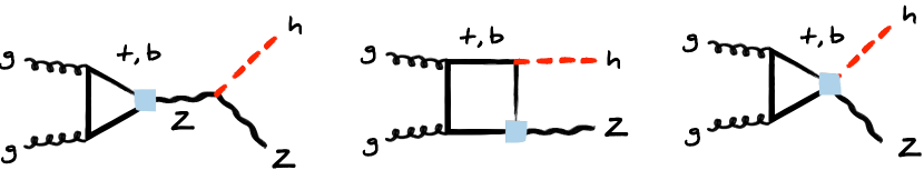
Figure 8: Examples of contributions to $gg\to Zh$ production within the SMEFT. All graphs involve an insertion of one of the operators given in (2) as indicated by the blue squares. Further details can be found in the main text.

It is important to realise that as a result of the generalised Furry theorem the vector-current coupling of the $Z$ boson, which is proportional to the combination $(g_{Zq}^{-}+g_{Zq}^{+})$ of couplings, does not contribute to the spin-averaged matrix element A0g2Z as given in (63). However, the axial-current part contributes, as signalled by the factor $(g_{Zq}^{-}-g_{Zq}^{+})$ in both (64) and (65), and this contribution is directly connected to the $U(1)_{A}\times SU(3)_{c}$ gauge anomaly. In fact, a regulator and a loop routing scheme must be introduced to properly define the amplitude ${\cal A}_{\texttt{A0g2Z}\triangle}^{q}$, rendering its expression scheme-dependent — for a detailed explanation of this point see for example Fox:2018ldq . Within the SM, the axial parts of the top- and bottom-quark couplings obey

$$(g_{Zt}^{-}-g_{Zt}^{+})=-(g_{Zb}^{-}-g_{Zb}^{+})\,,$$ (67)

and as a result all gauge anomalies are cancelled. It follows that the sum over $q$ that appears in (63) evaluates to

$$\sum_{q=t,b}\hskip 1.42262pt(g_{Zq}^{-}-g_{Zq}^{+})\hskip 1.42262pt{\cal A}_{\texttt{A0g2Z}\triangle}^{q}=(g_{Zt}^{-}-g_{Zt}^{+})\,\left({\cal A}_{\texttt{A0g2Z}\triangle}^{t}-{\cal A}_{\texttt{A0g2Z}\triangle}^{b}\right)\,,$$ (68)

and in consequence any scheme-dependent constant shift in the amplitude ${\cal A}_{\texttt{A0g2Z}\triangle}^{q}$ drops out in the combination $\big{(}{\cal A}_{\texttt{A0g2Z}\triangle}^{t}-{\cal A}_{\texttt{A0g2Z}\triangle}^{b}\big{)}$. Notice that in the degenerate or zero mass case the sum (68) vanishes identically. Since we treat the light-quark generations as massless, down-, up-, strange- and charm-quark loops hence do not need to be included in the spin-averaged matrix element (63).

The amplitudes including the SMEFT contributions to (63) were computed with the procedure outlined in Section 3.2. Since the SM amplitudes were derived in unitary gauge, only SMEFT contributions to vertices involving the $Z$ boson have to be considered. We have checked explicitly that in Feynman gauge, the SMEFT effects in the Goldstone diagrams are equivalent to the effects in the longitudinal part of the amplitude in unitary gauge. Another important point is that in the SMEFT, the coupling shifts $\delta g_{Zq}^{(0)\hskip 0.7113pt\pm}$ and $\delta g_{Zq}^{(1)\hskip 0.7113pt\pm}$ as given in (56) and (59), respectively, in general do not obey (67) and the scheme-dependent constant shift in ${\cal A}_{\texttt{A0g2Z}\triangle}^{q}$ thus does not automatically cancel in the sum (68). One may incorrectly jump to the conclusion that additional cancellation conditions analogous to (67) have to be imposed on the SMEFT Wilson coefficients in order to ensure the cancellation of gauge anomalies. However, one can show Bonnefoy:2020tyv ; Feruglio:2020kfq ; Cornella:2022hkc ; Cohen:2023gap ; Cohen:2023hmq that the anomalous contributions depending on the Wilson coefficients are “irrelevant”, in the sense that they can be removed by adding a local counterterm, i.e. a Wess-Zumino term Wess:1971yu . As a result, the condition for the cancellation of “relevant” gauge anomalies in the SMEFT is the same as in the SM and only dependent on the gauge quantum numbers of the fermionic sector, as one would naively expect from an effective field theory point of view. We cancel the unphysical terms in the amplitudes depicted in Figure 8 via the replacement

$${\cal A}_{\texttt{A0g2Z}\triangle}^{q}\,\to\,{\cal A}_{\texttt{A0g2Z}\triangle}^{q}-\lim_{m_{q}\to\infty}{\cal A}_{\texttt{A0g2Z}\triangle}^{q}\,,$$ (69)

for what concerns the SMEFT contribution to (63). Notice that for $m_{q}^{2}/s_{12}\to\infty$ the PV triangle integral appearing in (60) obeys $m_{q}^{2}\hskip 1.42262ptC_{0}(s_{12},0,0,m_{q},m_{q},m_{q})\to-1/2$ and hence the subtraction term in (69) is local and independent of the mass of the quark in the loop. Since the replacement (69) is the same for all $q$ in the sum appearing in A0g2Z, it drops out for an anomaly-free UV theory. At the same time the replacement ensures that ${\cal A}_{\texttt{A0g2Z}\triangle}^{q}$ decouples as $s_{12}/m_{q}^{2}$ in the limit $m_{q}^{2}\gg s_{12}$, recovering the behaviour obtained in the covariant anomaly scheme Bardeen:1984pm ; Fox:2018ldq ; Durieux:2018ggn ; Degrande:2020evl where the need for a local counterterm is circumvented by an adequate choice of the loop routing scheme. Notice that in contrast to the triangle contributions, the box corrections do not require a subtraction à la (69). An example SMEFT box graph is shown in the middle of Figure 8. It follows that, up to an overall factor of $2/v$, the counterterms necessary to remove the anomalous SMEFT contributions in the $ggZ$ and $gghZ$ vertices are identical.

Some additional care has to be taken regarding the SMEFT contributions to (63) from Feynman diagrams that involve an effective $hZq\bar{q}$ or $hZ\ell^{+}\ell^{-}$ vertex. A graph of the former type is depicted on the right in Figure 8. In these cases only the transversal part of (60) contributes — the longitudinal part vanishes because the $Z$ boson couples directly to the leptons that are treated as massless — and therefore in addition to dropping the factor $D_{Z}(s_{12})$ in (64), one also has to discard the longitudinal part in (60) by removing the factor $(1-s_{12}/m_{Z}^{2})$. This leads to the following contribution

$$\left[\frac{\left(\delta g_{hZq}^{(1)\hskip 0.7113pt-}-\delta g_{hZq}^{(1)\hskip 0.7113pt+}\right)g_{Z\ell}^{h_{\ell}}}{D_{Z}(s_{34})}+\frac{\left(g_{Zq}^{-}-g_{Zq}^{+}\right)\delta g_{hZ\ell}^{(1)\hskip 0.7113pth_{\ell}}}{D_{Z}(s_{12})}\right]\,\frac{{\cal A}_{\texttt{A0g2Z}\triangle}^{q}\left(1_{g}^{h_{g}},2_{g}^{h_{g}},3_{\ell}^{h_{\ell}},4_{\bar{\ell}}^{-h_{\ell}}\right)}{1-\frac{s_{12}}{m_{Z}^{2}}}\,,\hskip 22.76219pt$$ (70)

from SMEFT diagrams with a $hZq\bar{q}$ or $hZ\ell^{+}\ell^{-}$ vertex. This contribution can be included by simply adding the expression (70) to the sum over $q$ in (63). In order to cancel anomalous terms in the amplitude (70) one in addition has to include an appropriate counterterm contribution by applying (69) to (70).

We furthermore note that the amplitude for the generalised neutral current proportional to $\delta g_{hZZ}^{(1)}$ as given in (13) vanishes in A0g2Z. Also $\delta g_{h\gamma Z}^{(1)}$ and $\delta g_{h\gamma Z}^{(2)}$ have no effect, since the photon couples vectorially to the quark loop. Only $\delta g_{hZZ}^{(3)}$ as given in (57) and the corresponding SMEFT operators contribute to $gg\to Zh$ production. This contribution is however not anomalous and hence needs no special treatment. Let us finally mention that we have used OpenLoops 2 Buccioni:2019sur as well as the implementation SMEFT@NLO Degrande:2020evl together with MadGraph5_aMC@NLO Alwall:2014hca to cross check the results presented in this appendix.

Appendix C SMEFT effects at NLO$+$PS and NNLO$+$PS

NLO QCD correction to $Vh$ production in the SMEFT have been calculated by several groups Mimasu:2015nqa ; Degrande:2016dqg ; Alioli:2018ljm ; Bishara:2020vix ; Bishara:2020pfx ; Bishara:2022vsc . By now these computations can also be performed automatically by means of the combination of SMEFT@NLO and MadGraph5_aMC@NLO. In what follows, we will use the POWHEG-BOX implementation of $pp\to Zh\to\ell^{+}\ell^{-}h$ production presented in Alioli:2018ljm to obtain the relevant NLO$+$PS predictions. Our physics analysis proceeds as described in the first paragraph of Section 5.

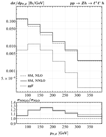
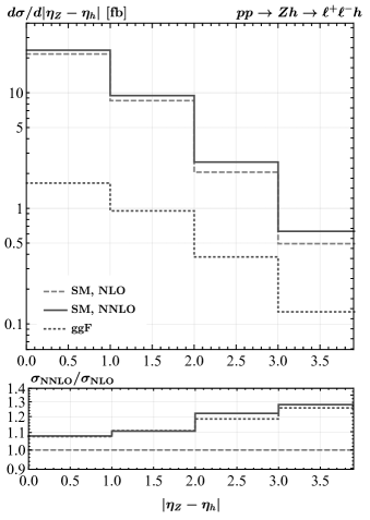
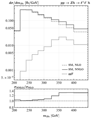
Figure 9: SM NLO$+$PS and NNLO$+$PS results for $pp\to Zh\to\ell^{+}\ell^{-}h$ production. The $|\eta_{Z}|$ (upper left), $p_{T,Z}$ (upper right), $|\eta_{Z}-\eta_{h}|$ (lower left) and $m_{Zh}$ (lower right) spectra are shown. The dashed (solid) lines illustrate the NLO$+$PS (NNLO$+$PS) results, while the dotted curves are the ggF NNLO$+$PS corrections. The solid (dotted) lines in the lower panels depict the ratios between the full NNLO$+$PS (NLO$+$PS plus ggF NNLO$+$PS) and the NLO$+$PS results. See main text for further explanations.

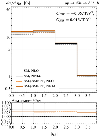
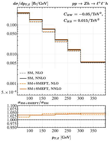
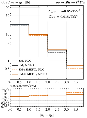
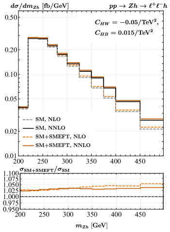
Figure 10: As Figure 9 but for benchmark scenario (45). The curves called SM+SMEFT correspond to the full squared matrix elements including the sum of both the SM and SMEFT contributions. The lower panels show the ratios between the SM+SMEFT and the SM predictions at the same order in QCD. For more details consult main text.

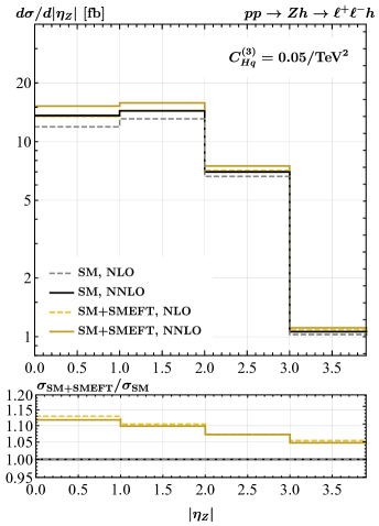
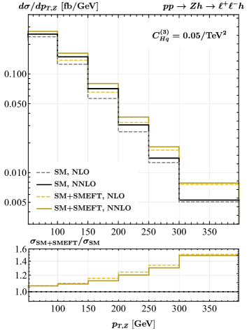
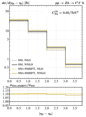
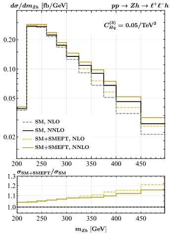
Figure 11: As Figure 10 but for benchmark scenario (47).

In Figure 9 we compare the SM predictions for the $|\eta_{Z}|$ (upper left), $p_{T,Z}$ (upper right), $|\eta_{Z}-\eta_{h}|$ (lower left) and $m_{Zh}$ (lower right) distribution in $pp\to Zh\to\ell^{+}\ell^{-}h$ production obtained at NLO$+$PS and NNLO$+$PS, respectively. The dashed (solid) lines correspond to the full NLO$+$PS (NNLO$+$PS) results, while the dotted curves depict the ggF contributions that start to contribute at NNLO$+$PS. From the displayed results it is evident that the NNLO corrections modify the NLO spectra in a non-trivial fashion. The relative size of the NNLO corrections amounts to less than $15\%$ in the $|\eta_{Z}|$ spectrum, while in the case of the $p_{T,Z}$, $|\eta_{Z}-\eta_{h}|$ and $m_{Zh}$ distributions the effects can reach up to around $30\%$. Notice that for the $p_{T,Z}$ spectrum the NNLO corrections are most pronounced in the vicinity of $p_{T,Z}\simeq m_{t}$, while in the case of $|\eta_{Z}-\eta_{h}|$ and $m_{Zh}$ the largest corrections arise in the tail of the distribution for $|\eta_{Z}-\eta_{h}|\gtrsim 3$ and $m_{Zh}\gtrsim 350\,{\rm GeV}$, respectively. The enhancement of the $p_{T,Z}$ spectrum at $p_{T,Z}\simeq m_{t}$ is related to the fact that for such transverse momenta the $Z$ boson is able to resolve the top-quark loop in the graph displayed on the right in Figure 2. In fact, another feature that is apparent from the solid and dashed lines in the lower panels is that within the SM the ggF NNLO effects are in general significantly larger than the ${\rm q\bar{q}F}$ NNLO counterparts.

The NLO$+$PS and NNLO$+$PS predictions corresponding to the SMEFT benchmark scenario (45) and (47) are given in Figure 10 and Figure 11, respectively. The dashed grey (solid black) histograms correspond to the NLO$+$PS (NNLO$+$PS) results in the SM, while the dashed (solid) coloured results are the corresponding SM+SMEFT predictions. One observes that while the NLO$+$PS and NNLO$+$PS results for the full predictions involving the squared matrix elements including the sum of both the SM and SMEFT contributions are notably different, the ratios between the SM+SMEFT and SM results turn out to be essentially independent on whether they are calculated at NLO or NNLO. In order to understand this feature one has to recall that in the SM the dominant NNLO corrections to $pp\to Zh\to\ell^{+}\ell^{-}h$ production arise from the $gg\to Zh$ channel, while the NNLO corrections associated to the $q\bar{q}\to Zh$ and $qg\to Zh$ channels are small. The opposite is the case in the SMEFT, where effects stemming from the $gg\to Zh$ channel are suppressed compared to the SM as a result of the additional subtraction (69). We add that the comparisons of SM+SMEFT predictions present in this appendix represent a non-trivial validation of our new NNLO$+$PS MC code for Higgsstrahlung.

References

- (1) ATLAS collaboration, Observation of decays and production with the ATLAS detector, Phys. Lett. B 786 (2018) 59 [1808.08238].
- (2) CMS collaboration, Observation of Higgs boson decay to bottom quarks, Phys. Rev. Lett. 121 (2018) 121801 [1808.08242].
- (3) ATLAS collaboration, Projections for measurements of Higgs boson cross sections, branching ratios, coupling parameters and mass with the ATLAS detector at the HL-LHC, ATL-PHYS-PUB-2018-054.
- (4) CMS collaboration, Sensitivity projections for Higgs boson properties measurements at the HL-LHC, CMS-PAS-FTR-18-011.
- (5) W. Buchmüller and D. Wyler, Effective Lagrangian Analysis of New Interactions and Flavor Conservation, Nucl. Phys. B268 (1986) 621.
- (6) B. Grzadkowski, M. Iskrzynski, M. Misiak and J. Rosiek, Dimension-Six Terms in the Standard Model Lagrangian, JHEP 10 (2010) 085 [1008.4884].
- (7) I. Brivio and M. Trott, The Standard Model as an Effective Field Theory, Phys. Rept. 793 (2019) 1 [1706.08945].
- (8) K. Mimasu, V. Sanz and C. Williams, Higher Order QCD predictions for Associated Higgs production with anomalous couplings to gauge bosons, JHEP 08 (2016) 039 [1512.02572].
- (9) C. Degrande, B. Fuks, K. Mawatari, K. Mimasu and V. Sanz, Electroweak Higgs boson production in the standard model effective field theory beyond leading order in QCD, Eur. Phys. J. C 77 (2017) 262 [1609.04833].
- (10) S. Alioli, W. Dekens, M. Girard and E. Mereghetti, NLO QCD corrections to SM-EFT dilepton and electroweak Higgs boson production, matched to parton shower in POWHEG, JHEP 08 (2018) 205 [1804.07407].
- (11) F. Bishara, P. Englert, C. Grojean, M. Montull, G. Panico and A.N. Rossia, A New Precision Process at FCC-hh: the diphoton leptonic channel, JHEP 07 (2020) 075 [2004.06122].
- (12) F. Bishara, S. De Curtis, L. Delle Rose, P. Englert, C. Grojean, M. Montull et al., Precision from the diphoton channel at FCC-hh, JHEP 04 (2021) 154 [2011.13941].
- (13) F. Bishara, P. Englert, C. Grojean, G. Panico and A.N. Rossia, Revisiting at the LHC and FCC-hh, JHEP 06 (2023) 077 [2208.11134].
- (14) R. Gauld, B.D. Pecjak and D.J. Scott, One-loop corrections to and decays in the Standard Model Dimension-6 EFT: four-fermion operators and the large- limit, JHEP 05 (2016) 080 [1512.02508].
- (15) R. Gauld, B.D. Pecjak and D.J. Scott, QCD radiative corrections for in the Standard Model Dimension-6 EFT, Phys. Rev. D 94 (2016) 074045 [1607.06354].
- (16) J.M. Cullen, B.D. Pecjak and D.J. Scott, NLO corrections to decay in SMEFT, JHEP 08 (2019) 173 [1904.06358].
- (17) J.M. Cullen and B.D. Pecjak, Higgs decay to fermion pairs at NLO in SMEFT, JHEP 11 (2020) 079 [2007.15238].
- (18) U. Haisch, D.J. Scott, M. Wiesemann, G. Zanderighi and S. Zanoli, NNLO event generation for production in the SM effective field theory, JHEP 07 (2022) 054 [2204.00663].
- (19) F. Maltoni, K. Mawatari and M. Zaro, Higgs characterisation via vector-boson fusion and associated production: NLO and parton-shower effects, Eur. Phys. J. C 74 (2014) 2710 [1311.1829].
- (20) A. Greljo, G. Isidori, J.M. Lindert, D. Marzocca and H. Zhang, Electroweak Higgs production with HiggsPO at NLO QCD, Eur. Phys. J. C 77 (2017) 838 [1710.04143].
- (21) W. Bizoń, F. Caola, K. Melnikov and R. Röntsch, Anomalous couplings in associated production with Higgs boson decay to massive quarks at NNLO in QCD, Phys. Rev. D 105 (2022) 014023 [2106.06328].
- (22) S. Alioli, P. Nason, C. Oleari and E. Re, A general framework for implementing NLO calculations in shower Monte Carlo programs: the POWHEG BOX, JHEP 06 (2010) 043 [1002.2581].
- (23) P.F. Monni, P. Nason, E. Re, M. Wiesemann and G. Zanderighi, MiNNLOPS: a new method to match NNLO QCD to parton showers, JHEP 05 (2020) 143 [1908.06987].
- (24) P.F. Monni, E. Re and M. Wiesemann, MiNNLO: optimizing hadronic processes, Eur. Phys. J. C 80 (2020) 1075 [2006.04133].
- (25) I. Majer, Associated Higgs Boson Production at NNLO QCD, Ph.D. thesis, ETH Zurich, 2020, 10.3929/ethz-b-000448848.
- (26) G. Kramer and B. Lampe, Two Jet Cross-Section in Annihilation, Z. Phys. C 34 (1987) 497.
- (27) R. Hamberg, W.L. van Neerven and T. Matsuura, A complete calculation of the order correction to the Drell-Yan factor, Nucl. Phys. B 359 (1991) 343.
- (28) T. Gehrmann and L. Tancredi, Two-loop QCD helicity amplitudes for and , JHEP 02 (2012) 004 [1112.1531].
- (29) J.M. Campbell, R.K. Ellis and C. Williams, Associated production of a Higgs boson at NNLO, JHEP 06 (2016) 179 [1601.00658].
- (30) O. Brein, R. Harlander, M. Wiesemann and T. Zirke, Top-Quark Mediated Effects in Hadronic Higgs-Strahlung, Eur. Phys. J. C 72 (2012) 1868 [1111.0761].
- (31) S. Zanoli, M. Chiesa, E. Re, M. Wiesemann and G. Zanderighi, Next-to-next-to-leading order event generation for production with decay, JHEP 07 (2022) 008 [2112.04168].
- (32) L.J. Dixon, Calculating scattering amplitudes efficiently, in Theoretical Advanced Study Institute in Elementary Particle Physics (TASI 95): QCD and Beyond, pp. 539–584, 1, 1996 [hep-ph/9601359].
- (33) D. Maitre and P. Mastrolia, S@M, a Mathematica Implementation of the Spinor-Helicity Formalism, Comput. Phys. Commun. 179 (2008) 501 [0710.5559].
- (34) R. Gauld, U. Haisch, L. Schnell, Vh Amplitudes, https://gitlab.com/lucschnell/vh-amplitudes [Accessed: 2023-11-03].
- (35) Particle Data Group collaboration, Review of Particle Physics, PTEP 2022 (2022) 083C01.
- (36) T. Gehrmann and E. Remiddi, Two loop master integrals for 3 jets: The Planar topologies, Nucl. Phys. B 601 (2001), 248-286 [hep-ph/0008287].
- (37) T. Gehrmann and E. Remiddi, Numerical evaluation of two-dimensional harmonic polylogarithms, Comput. Phys. Commun. 144 (2002), 200-223 [hep-ph/0111255].
- (38) T. Hahn and M. Perez-Victoria, Automatized one loop calculations in four-dimensions and D-dimensions, Comput. Phys. Commun. 118 (1999), 153-165 [hep-ph/9807565].
- (39) K. Hagiwara and D. Zeppenfeld, Amplitudes for Multiparton Processes Involving a Current at , , and Hadron Colliders, Nucl. Phys. B 313 (1989), 560-594
- (40) K. Hasegawa, S. Moch and P. Uwer, AutoDipole: Automated generation of dipole subtraction terms, Comput. Phys. Commun. 181 (2010), 1802-1817 [0911.4371].
- (41) W. Astill, W. Bizoń, E. Re and G. Zanderighi, NNLOPS accurate associated production with decay at NLO, JHEP 11 (2018) 157 [1804.08141].
- (42) S. Alioli, A. Broggio, S. Kallweit, M.A. Lim and L. Rottoli, Higgsstrahlung at NNLLNNLO matched to parton showers in GENEVA, Phys. Rev. D 100 (2019) 096016 [1909.02026].
- (43) W. Bizoń, E. Re and G. Zanderighi, NNLOPS description of the decay with MiNLO, JHEP 06 (2020) 006 [1912.09982].
- (44) P. Nason, A New method for combining NLO QCD with shower Monte Carlo algorithms, JHEP 11 (2004) 040 [hep-ph/0409146].
- (45) S. Frixione, P. Nason and C. Oleari, Matching NLO QCD computations with Parton Shower simulations: the POWHEG method, JHEP 11 (2007) 070 [0709.2092].
- (46) T. Sjöstrand, S. Ask, J.R. Christiansen, R. Corke, N. Desai, P. Ilten et al., An introduction to PYTHIA 8.2, Comput. Phys. Commun. 191 (2015) 159 [1410.3012].
- (47) R. Boughezal, J.M. Campbell, R.K. Ellis, C. Focke, W. Giele, X. Liu et al., Color singlet production at NNLO in MCFM, Eur. Phys. J. C 77 (2017) 7 [1605.08011].
- (48) R. Gauld, A. Gehrmann-De Ridder, E.W.N. Glover, A. Huss and I. Majer, Associated production of a Higgs boson decaying into bottom quarks and a weak vector boson decaying leptonically at NNLO in QCD, JHEP 10 (2019) 002 [1907.05836].
- (49) F. Buccioni, J.-N. Lang, J.M. Lindert, P. Maierhöfer, S. Pozzorini, H. Zhang et al., OpenLoops 2, Eur. Phys. J. C 79 (2019) 866 [1907.13071].
- (50) S. Frixione, Z. Kunszt and A. Signer, Three jet cross-sections to next-to-leading order, Nucl. Phys. B 467 (1996) 399 [hep-ph/9512328].
- (51) S. Frixione, A General approach to jet cross-sections in QCD, Nucl. Phys. B 507 (1997) 295 [hep-ph/9706545].
- (52) S. Dawson and P.P. Giardino, Electroweak and QCD corrections to and pole observables in the standard model EFT, Phys. Rev. D 101 (2020) 013001 [1909.02000].
- (53) K. Hamilton, P. Nason and G. Zanderighi, MINLO: Multi-Scale Improved NLO, JHEP 10 (2012) 155 [1206.3572].
- (54) K. Hamilton, P. Nason, C. Oleari and G. Zanderighi, Merging and jet at NLO with no merging scale: a path to parton shower + NNLO matching, JHEP 05 (2013) 082 [1212.4504].
- (55) L. Chen and A. Freitas, Mixed EW-QCD leading fermionic three-loop corrections at to electroweak precision observables, JHEP 03 (2021) 215 [2012.08605].
- (56) ALEPH, DELPHI, L3, OPAL, SLD, LEP Electroweak Working Group, SLD Electroweak Group, SLD Heavy Flavour Group collaboration, Precision electroweak measurements on the resonance, Phys. Rept. 427 (2006) 257 [hep-ex/0509008].
- (57) A. Falkowski and D. Straub, Flavourful SMEFT likelihood for Higgs and electroweak data, JHEP 04 (2020) 066 [1911.07866].
- (58) I. Brivio, SMEFTsim 3.0 — a practical guide, JHEP 04 (2021) 073 [2012.11343].
- (59) LHC Higgs Cross section Working Group collaboration, https://twiki.cern.ch/twiki/bin/view/LHCPhysics/CERNYellowReportPageBR.
- (60) ATLAS collaboration, A combination of measurements of Higgs boson production and decay using up to 139 fb-1 of proton-proton collision data at = 13 TeV collected with the ATLAS experiment, ATLAS-CONF-2020-027.
- (61) CMS collaboration, Combined Higgs boson production and decay measurements with up to 137 fb-1 of proton-proton collision data at = 13 TeV, CMS-PAS-HIG-19-005.
- (62) ATLAS and CMS collaborations, Evidence for the Higgs boson decay to a boson and a photon at the LHC, [2309.03501].
- (63) NNPDF collaboration, Parton distributions from high-precision collider data, Eur. Phys. J. C 77 (2017) 663 [1706.00428].
- (64) P. Skands, S. Carrazza and J. Rojo, Tuning PYTHIA 8.1: the Monash 2013 Tune, Eur. Phys. J. C 74 (2014) 3024 [1404.5630].
- (65) ATLAS collaboration, Measurement of , production as a function of the vector-boson transverse momentum in 13 TeV collisions with the ATLAS detector, JHEP 05 (2019) 141 [1903.04618].
- (66) ATLAS collaboration, Measurements of and production in the decay channel in collisions at 13 TeV with the ATLAS detector, Eur. Phys. J. C 81 (2021) 178 [2007.02873].
- (67) CMS collaboration, Simplified template cross section measurements of Higgs boson produced in association with vector bosons in the decay channel in proton-proton collisions at =13 TeV, CMS-PAS-HIG-20-001.
- (68) The POWHEG BOX, http://powhegbox.mib.infn.it.
- (69) J.R. Andersen et al., Les Houches 2015: Physics at TeV Colliders Standard Model Working Group Report, in 9th Les Houches Workshop on Physics at TeV Colliders, 5, 2016 [1605.04692].
- (70) N. Berger et al., Simplified Template Cross Sections - Stage 1.1, [1906.02754].
- (71) S. Amoroso et al., Les Houches 2019: Physics at TeV Colliders: Standard Model Working Group Report, in 11th Les Houches Workshop on Physics at TeV Colliders: PhysTeV Les Houches, 3, 2020 [2003.01700].
- (72) C. Degrande, G. Durieux, F. Maltoni, K. Mimasu, E. Vryonidou and C. Zhang, Automated one-loop computations in the standard model effective field theory, Phys. Rev. D 103 (2021) 096024 [2008.11743].
- (73) A. Biekötter, B.D. Pecjak, D.J. Scott and T. Smith, Electroweak input schemes and universal corrections in SMEFT, JHEP 07 (2023) 115 [2305.03763].
- (74) T. Hahn, S. Paßehr and C. Schappacher, FormCalc 9 and Extensions, PoS LL2016 (2016) 068 [1604.04611].
- (75) P.J. Fox, I. Low and Y. Zhang, Top-philic forces at the LHC, JHEP 03 (2018) 074 [1801.03505].
- (76) Q. Bonnefoy, L. Di Luzio, C. Grojean, A. Paul and A.N. Rossia, Comments on gauge anomalies at dimension-six in the Standard Model Effective Field Theory, JHEP 05 (2021) 153 [2012.07740].
- (77) F. Feruglio, A Note on Gauge Anomaly Cancellation in Effective Field Theories, JHEP 03 (2021) 128 [2012.13989].
- (78) C. Cornella, F. Feruglio and L. Vecchi, Gauge invariance and finite counterterms in chiral gauge theories, JHEP 02 (2023) 244 [2205.10381].
- (79) T. Cohen, X. Lu and Z. Zhang, Anomalies from the covariant derivative expansion, Phys. Rev. D 107 (2023) 116015 [2301.00821].
- (80) T. Cohen, X. Lu and Z. Zhang, Anomaly cancellation in effective field theories from the covariant derivative expansion, Phys. Rev. D 108 (2023) 056027 [2301.00827].
- (81) J. Wess and B. Zumino, Consequences of anomalous Ward identities, Phys. Lett. B 37 (1971) 95.
- (82) W.A. Bardeen and B. Zumino, Consistent and Covariant Anomalies in Gauge and Gravitational Theories, Nucl. Phys. B 244 (1984) 421.
- (83) G. Durieux, J. Gu, E. Vryonidou and C. Zhang, Probing top-quark couplings indirectly at Higgs factories, Chin. Phys. C 42 (2018) 123107 [1809.03520].
- (84) J. Alwall, R. Frederix, S. Frixione, V. Hirschi, F. Maltoni, O. Mattelaer et al., The automated computation of tree-level and next-to-leading order differential cross sections, and their matching to parton shower simulations, JHEP 07 (2014) 079 [1405.0301].