Charting multidimensional ideological polarization across demographic groups
in the United States

Abstract

The causes for the rise in affective polarization are debated, primarily revolving around ideological polarization and partisan sorting hypotheses. The former indicates divergent ideological beliefs on key issues as the main fuel for the increasing political divide. The latter, instead, proposes that the alignment of social identity with partisan affiliation intensifies partisan rift. We present a novel methodology using data from the American National Election Studies (ANES) to discern the contributions of both ideological polarization and partisan sorting to affective polarization. We quantify multidimensional polarization by embedding ANES respondents to a variety of political, social, and economic topics into a two-dimensional ideological space. We identify several demographic attributes (Race, Gender, Age, Affluence, and Education) of the ANES respondents to measure their alignment with partisan affiliation. Our results show that income and especially racial groups are strongly sorted into parties, while education is orthogonal to partisanship. By analyzing the trajectories of political and demographic groups across time, we observe an increasing partisan divide, due to both parties moving away from the center at different rates. Opinions within groups become increasingly heterogeneous in the last decade, with a share of Democratic voters moving to a novel region of the ideological space. We conclude that the observed growth in partisan divide is due to a combination of partisan sorting and increasing ideological polarization, mainly occurring after 2010.

Affective polarization —the situation where individuals develop favorable sentiments toward members of their own political party or group and negative feelings toward the opposing party— has been widely observed in the United States Iyengar et al. (2019); Iyengar and Westwood (2015); Druckman et al. (2021) and other countries Boxell et al. (2022). Affective (or social Banda and Cluverius (2018)) polarization can exacerbate the widening political gap in our society Iyengar et al. (2012), fueling distrust in democratic institutions, and impeding collaborative efforts to address crucial societal issues Wang et al. (2020). The causes of this phenomenon are widely debated, and two main hypotheses have been formulated.

Affective polarization may be driven by ideological (or issue) polarization, i.e., individuals having increasingly divergent beliefs on ideological issues, such as abortion or affirmative action Rogowski and Sutherland (2016); Webster and Abramowitz (2017). Some scholars pointed out social media as an underlying root for this increasing disagreement Bail et al. (2018); Van Bavel et al. (2021). Recommendation algorithms, in particular, are suspected to reinforce ideological segregation Santos et al. (2021), reducing engagement with information from opposing viewpoints, a phenomenon known as echo-chambers Baumann et al. (2020); Cinelli et al. (2021); Diaz-Diaz et al. (2022). Very recently, however, this hypothesis has been disputed, after observing that changing Facebook’s feed algorithm to reduce exposure to like-minded content does not seem to reduce the political polarization of users González-Bailón et al. (2023); Guess et al. (2023a, b); Nyhan et al. (2023).

Alternatively, some political scientists believe that partisan-ideological sorting, by which people sort into the “correct” combination of party and ideology Mason (2015), increased the strength of partisan social identity and thus contributed to the political divide Mason (2016); West and Iyengar (2022). Within this framework, groups with strong social identities, such as racial, religious, or ideological identities, firmly align with parties in recent decades Egan (2020). For instance, the average correlations between different issue attitudes and party identification (Democratic or Republican) between 1972 and 2004 increased by 5% per decade Baldassarri and Gelman (2008). Other studies found correlations with race and religion, being black and atheist Americans aligned with the Democratic party, while white and Christian groups with the Republican party Mason and Wronski (2018). Likewise, Americans with higher incomes tend to hold more conservative preferences on economic policy, but more liberal stances on social policy, and vice versa Wright and Rigby (2020). Interestingly, online interactions on social media have been shown to be segregated by demographic factors Monti et al. (2023), and contribute to the rise of affective polarization through partisan sorting Törnberg (2022).

To discern these underlying factors, researchers from different disciplines, ranging from political and social science to physics and computer science, have recently embarked on the endeavor of quantifying ideological polarization Guerra et al. (2013); Boxell et al. (2017); Waller and Anderson (2021). On the one hand, they leverage data from social media to define new methodologies to measure the extent of polarization Morales et al. (2015); Garimella et al. (2018); Hohmann et al. (2023). However, social media users are usually not representative of the whole population Zagheni and Weber (2015). For instance, Facebook and Twitter users are demographically biased, being younger, more liberal, and better educated on average Mellon and Prosser (2017). On the other hand, several measures of ideological polarization and partisan sorting have been proposed on offline data Miller and Conover (2015); Davis and Dunaway (2016); Iyengar and Krupenkin (2018). However, these methods are mainly based on self-reported surveys, often including substantial measurement error due to social desirability bias Brenner and DeLamater (2016). Similarly, partisanship measured by self-reported scores might be biased, even by the structure of the questionnaire itself Schiff et al. (2022). Furthermore, most of these works encompass single topics, while ideological polarization is by nature multidimensional Baumann et al. (2021); Pedraza et al. (2021), embracing multiple concepts at the same time Bramson et al. (2016). When dealing with several topics simultaneously, the discrete nature of the Likert scale used to assess opinions makes it even harder to interpolate ideological polarization.

In this paper, we propose a novel methodology to disentangle the alternative hypotheses for the increase of affective polarization, by quantifying partisan sorting and the evolution of ideological polarization. To this aim, we embed the respondents of the American National Election Studies (ANES) ane , encompassing opinions regarding a large number of political, social, and economic topics, into a two-dimensional ideological space. There, we can gauge polarization by simply measuring the Euclidean distance between opposite political and demographic groups. We focus on party identification (Democratic or Republican parties) and five demographic attributes (Race, Gender, Age, Affluence, and Education). The opinion embedding allows us to quantify the multidimensional polarization of the ANES respondent, simultaneously with respect to many different topics. We chart partisan sorting in the ideological space, depicted as the alignment (measured by the gradient vector of opinions) between parties and different demographic groups. Our results confirm that the partisanship divide has increased, particularly in the last decade, while income and especially racial groups are strongly sorted into parties. However, we find that part of the increased partisan segregation is due to a rise in ideological polarization: A share of Democratic voters occupied a novel region of the ideological space in recent years, connected with opinions regarding minority rights.

Results

We focus on the ANES surveys conducted in the years 1992, 2000, 2008, 2016, and 2020. The last five United States Presidents were elected these years: Clinton (Democratic), Bush (Republican), Obama (D), Trump (R), Biden (D). We preprocess data in order to select common questions among these years related to different topics such as the state of the economy, government spending, religion, or minority rights, see Materials and Methods for details. Our working dataset consists in $N=11614$ respondents answering 29 different questions.

Embedding opinions into an ideological space

The simplest data representation is a multidimensional space containing 11614 points (respondents) in 29 dimensions (questions). Each data point corresponds to a vector in the space of the 29 questions selected (forming the axes), representing the opinion of a single respondent. However, this high-dimensional representation is extremely sparse, incurring the curse of dimensionality Houle et al. (2010). Indeed, as the number of dimensions increases, the volume of available space grows exponentially and every data point becomes increasingly separate from the rest. As a consequence, distance metrics like Euclidean distance lose their usefulness in high-dimensional spaces Altman and Krzywinski (2018). Similarly, sparse data in high dimensions hinder downstream machine learning applications Radovanović et al. (2010). For instance, they affect the meaning of proximity or nearest neighbor, since the distance between any two points becomes more and more similar Aggarwal et al. (2001).

Therefore, we reduce the dimensionality of the data representation while retaining the original geometry as much as possible, by performing an opinion embedding into a two-dimensional ideological space. The opinion embedding allows us to chart and quantify ideological polarization by using a simple Euclidean distance. Furthermore, it allows us to interpolate the discrete nature of the original data, where opinions are expressed in the Likert scale, into a continuous ideological space. Similar dimensionality reduction methods have been used to map the opinion similarity and ideological leaning of Internet users Faridani et al. (2010); Monti et al. (2021), as well as the scientific knowledge landscape into a low-dimensional spatial representation Chinazzi et al. (2019); Singh et al. (2023). By studying the embedding trajectories of users in this space one can, for instance, predict their future evolution in time Kumar et al. (2019).

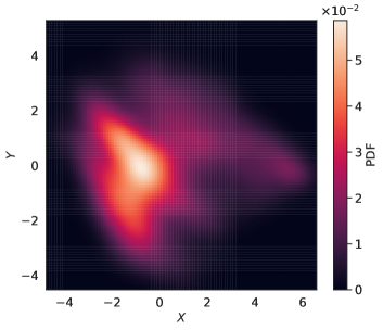
Figure 1: Probability density function (PDF) of the ANES respondents in the two-dimensional ideological space obtained by Isomap with $K=10$. The lighter (darker) areas are the ones with greater (lower) density. The $X$- and $Y$-axes of the ideological space are arbitrary, combinations of the 29 questions selected.

In this work, we implement Isomap Tenenbaum et al. (2000), a non-linear, quasi-isometric, low-dimensional embedding algorithm (see Materials and Methods for more details), to obtain a two-dimensional data representation. We opt for a non-linear dimensionality reduction algorithm in order to preserve the local structure of the high-dimensional data Saul and Roweis (2003). Since we select the same set of 29 questions for each year, we are able to embed all opinions across years into the same ideological space, where we can study the temporal evolution of opinions. The two axes of the ideological space represent a (non-linear) combination of the 29 questions selected. In Fig. 1 we plot the density of respondents: A brighter (darker) color indicates areas with a higher (lower) density of individuals. While some regions of the space are much denser than others, indicating that many individuals share similar opinions, one can also see less populated areas. Note that the spatial orientation of the embedding is arbitrary, being the distance between points the only meaningful information: The larger the distance between two individuals, the less akin their opinions.

We checked that the opinion embedding does not lose part of the information contained in the original data, by comparing the accuracy of a classification algorithm on original and embedded data. We predict the political leaning of respondents (Republican or Democratic) by using logistic regression informed by i) their responses to the full set of 29 questions, and ii) their coordinates in the ideological space. The ten-fold cross-validated balanced accuracy reads $0.76\pm 0.06$ for original data, and $0.75\pm 0.06$ for embedded data (see Materials and Methods for details). Furthermore, we tested that our findings (shown in the following) do not depend on the specific embedding representation, by using a different value of the Isomap hyperparameter $K$ and by implementing a different, linear embedding algorithm, the Principal Component Analysis (PCA) Jolliffe (2002), see Supplementary Material (SM).

Polarization across socio-demographic groups

Attribute	Groups
Party	Democrats	Republicans
Race	Black	White
Gender	Female	Male
Age	17-34	55+
Affluence	Low-Income	High-Income
Education	No-College	College

Table 1: Classification of the respondents by attributes according to two opposite groups.

To compare the opinions of different groups of individuals, we leverage the rich metadata in the ANES survey to identify five demographic attributes (Race, Gender, Age, Affluence, and Education) and the political leaning of the respondents. We select two opposite groups per attribute, reported in Table 1, in order to highlight the differences in their opinions. For instance, we consider Low-Income and High-Income groups if the respondent belongs to a percentile lower than 34% or higher than 66%, respectively, of the American income distribution. Individuals in the middle-income group are excluded. With respect to the political leaning, we consider Democrats and Republicans (as per self-attribution in ANES data) excluding individuals classified as Independents. Fig. 3 in the SM shows the proportion of each group for the different attributes, over the years.

Fig. 2 shows the density distribution of opposite groups in the ideological space, for different attributes. For each attribute, we assign a binary variable $\{+1,-1\}$ to opposite groups, e.g., a value $+1$ to Republicans and $-1$ to Democrats. We then divide the ideological space in a lattice of small cells and compute the average of the binary variable in each cell. Cells with a large majority of one group are colored by darker colors, while cells in lighter colors are populated by roughly the same number of individuals of the two groups. For instance, in Fig. 2(a), dark red (blue) cells are mostly populated by Republicans (Democrats).

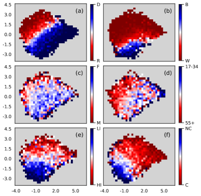
Figure 2: Density distribution of opposite groups in the ideological space, for different attributes: (a) Democrats (D) and Republicans (R), (b) Black (B) and White (W), (c) Female (F) and Male (M), (d) aged 17-34 and 55+, (e) Low-Income (LI) and High-Income (HI), (f) No-College degree (NC) and College (C). Darker (lighter) cells have a strong (weak) prevalence of one group with respect to the other. Cells with no respondents are colored in gray. We bin the ideological space into 36 $\times$ 29 cells. We slightly smooth data by applying a different Gaussian filter with a low standard deviation for each attribute.

One can see that the opinions of different groups are not randomly distributed in the space, but rather ordered for most attributes. The attributes of Party, Race, Affluence, and Education show the most ordered distributions, with opposite groups well separated in the ideological space, while the opinion distribution with respect to Gender and Age are much more uniform. This indicates that Republicans and Democrats, for instance, have different and often opposite opinions with respect to the 29 questions selected. While this observation can be checked at the level of the single question, our method allows us a bird-eye view of ideological polarization with respect to many different topics at the same time.

Furthermore, not only opposite groups are segregated in the ideological space, but they are also ordered along a certain direction. The Black, Low-Income, and No-College groups mostly populate the bottom region of the embedding, whereas the White, High-Income, and College groups are mostly present at the top of it. This observation can be quantified by computing the gradient of the different opinion distributions throughout the ideological space. For each cell of Fig. 2, we compute the direction and rate of the fastest increase of the average opinion. We use finite differences to approximate the derivatives of the gradient with high accuracy. We define the gradient of the opinion distribution as the vector sum of the gradient values of each cell. A longer (shorter) gradient vector is obtained, thus, if the opinion distribution is more (less) ordered along a certain direction.

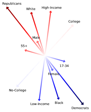
Figure 3: Gradient vectors for each attribute computed from their opinion distribution shown in Fig. 2. We discarded cells with less than 10 respondents. The blue-red colormap obtained for the Party attribute is used, with Republicans in dark red and Democrats in dark blue. The vectors are colored according to the Republicans-Democrats axis, i.e., the color of each point in the vectors is proportional to the radius times the cosine of their angle with the Republicans-Democrats axis.

Fig. 3 shows the resulting gradients for each attribute, indicating that groups whose opinions are more polarized are Democrats vs Republicans, Low-Income vs High-Income, Black vs White, and No-College vs College, in this order. The attributes of Gender and Age, instead, show little polarization, as indicated by short gradient vectors. In Fig. 3, we color each vector by the Party colormap, with Republicans in dark red and Democrats in dark blue. The remaining vectors are colored according to the Republicans-Democrats axis. As a consequence, the Education (College to No-College) vector, almost orthogonal to the Party one, is very lightly colored.

The gradient vectors are useful to quantify the partisan sorting of different demographic groups. Party and Race gradient vectors point in similar directions, indicating that the opinions of Black (White) individuals overlap, to a certain extent, with those of Democrats (Republicans). The same observation partially holds for the Affluence attribute, opinions of High-Income (Low-Income) individuals are more similar to Republicans (Democrats). Instead, the Education vector is almost orthogonal to the Party one, indicating little partisan sorting with respect to Education. Therefore, one could identify the Party-Education attributes as the two main axes of the ideological space, and express the likelihood of individuals to belong to the four groups defined by these axes. Individuals in the upper (lower) region of the ideological space are more likely to be Republicans (Democrats) with (without) a college degree. Looking at Fig. 2(b) and (e), one can see that this upper (lower) region is mostly populated by White (Black) and High-Income (Low-Income) individuals.

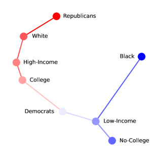
Figure 4: Minimum spanning tree (MST) of the ideological affinity among groups of Party, Race, Affluence, and Education. The MST connects all groups by the edges minimizing the total KS distance between them. The length of edges, as well as the blue-red colormap, are proportional to the KS distance. The position of the nodes is arbitrary.

The correlation between the opinions of different demographic groups observed so far can be quantified more precisely. We identify the opinion distribution in the ideological space of the 8 most polarized groups (corresponding to Party, Race, Affluence, and Education attributes). Then, we compare all pairs by means of the two-dimensional Kolmogorov-Smirnov (KS) test Peacock (1983), which provides the distance $D_{KS}$ between two distributions. Fig. 4 in the SM shows that the groups with the shortest KS distance are High-Income and College. These groups show a similar opinion distribution in the ideological space, i.e., they show a certain degree of ideological affinity Bush (2017); Martin-Gutierrez et al. (2023). We visualize this intuition by obtaining a hierarchical diagram connecting the most similar groups. Fig. 4 shows the minimum spanning tree (MST) obtained by the KS distance between groups. The MST is constructed by connecting pairs of groups with edges, such that all groups are connected, there are no cycles, and the total distance between groups joined by edges is the minimum possible. In Fig. 4, the length of the edges is proportional to the KS distance between nodes. The two nodes with the largest distance (Black and Republicans) are colored with the darkest colors, while the rest of the nodes are colored according to their distance from these two groups. Fig. 4 shows that different socio-demographic groups can be ordered in terms of ideological affinity, from Republican, White, and High-Income groups to Low-Income, No-College, and Black groups. From the Figure, we recover the tendency observed in Fig. 2, where White and High-Income are located at the top region of the ideological space, while Black and Low-Income groups populate the bottom regions.

Charting ideological trajectories in time

Next, we study the temporal evolution of the opinions of different groups over 30 years. To this aim, we start by considering a coarse-grained quantity to capture the aggregate behavior of different socio-demographic groups. We consider the centroid (or geometric center) of each group in each year, defined as the arithmetic mean position of the opinions of the group, indicating the average group opinion. Fig. 5 shows the Euclidean distance between the centroids of opposite groups, for each attribute across the years. We remark that we do not compare distances between different opinion embeddings for each year, but we instead consider different groups within the same ideological space. First, we note that the distance between the centroids is proportional to the KS distance, defined in the previous paragraph (see Fig. 5 in the SM). This observation confirms that the closer two groups are in the ideological space, the more similar their opinion distributions, a sign of ideological affinity. From Fig. 5 we see that the groups in Party, Race, Affluence, and Education show larger distances, indicating that they are more polarized. This corroborates the results shown in Figs. 2 and 3: The attributes with the largest centroid distance correspond to the most ordered opinion distributions with the longest gradient vectors. While most centroid distances do not vary much over time, one can observe a notable exception for the Party groups: The disagreement between Democrats and Republicans has considerably increased over time, overcoming the ideological separation between racial groups after 2008. This observation indicates a much more polarized environment in 2016 and especially in 2020 with respect to earlier years.

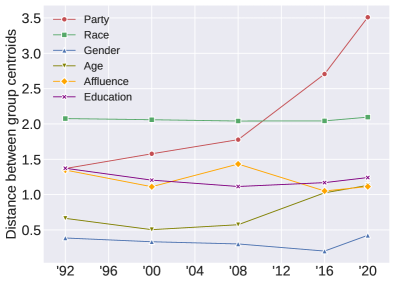
Figure 5: Euclidean distance between the average opinions (centroids) of the opposite groups of each attribute, for every year.

In order to check that the centroid distances are statistically significant, we build a null model assuming that opinions do not differ across groups. More specifically, we run a bootstrap analysis for each attribute, by randomly assigning each data point to one of the two groups while preserving their proportion. We repeat this process $10^{5}$ times for each attribute, obtaining the centroids of the two opposite groups in every iteration. We assume that this sample of centroids follows a bivariate normal distribution. The distance $R$ between the observed centroid and such a two-dimensional distribution is defined as the Mahalanobis distance. In Materials and Methods we show that, if the null hypothesis (opinions do not differ across groups) is correct, the probability of obtaining a centroid distribution compatible with the observed centroids (p-value Fisher (1955)) is given by $p\left(R\right)=\mathrm{e}^{-R^{2}/2}$. We found that the p-values corresponding to the less polarized attributes are greater than the ones corresponding to the most polarized attributes. The largest p-value is obtained for Gender in 2016 (equal to $p=0.016$), the p-value of Gender and Age is lower than $10^{-4}$ in the rest of the years, while Party, Race, Affluence, and Education show a p-value always lower than $10^{-10}$. This finding indicates that most socio-demographic groups are characterized by different, and in some cases very distant, opinions, as also indicated by the KS test.

While the centroid distance provides relevant information regarding the relative displacement of the two groups within the ideological space, we are also interested in charting the trajectory of each group across time. With this aim, we study the evolution of the position of the average opinion of the most polarized groups (Party, Race, Affluence, and Education) in different years in the ideological space. First, we note that the average opinion of the general population varies across time, especially in 2008 and 2020 (see Fig. 6 in the SM). Therefore, to meaningfully compare the trajectory of each group, in Fig. 6 we discard such a drift by subtracting the average population opinion from each group, for every year. In this way, we can see if groups move closer or not to the average population opinion, located at (0,0) in the Figure.

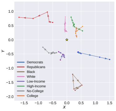
Figure 6: Average opinion (centroid) of the Party, Race, Affluence, and Education groups across years in the ideological space. The centroids are linked by arrows in chronological sequence. The average opinion of the population of each year is subtracted from each group, being located at (0,0) and marked with a star. As in Fig. 1, the $X$- and $Y$-axes are arbitrary, combinations of the 29 questions selected.

Note that we recover the spatial disposition of the groups in the ideological space found in Figs. 2 and 3: Republicans, White, High-Income, and College groups are located in the upper region above the center (0,0), whereas we find their counterparts at the bottom. While most groups orbit in the ideological space without moving much across years, we note two notable exceptions. First, the average opinions of the Black group and the general population were particularly similar in 2008. This could be the result of the “Obama Effect” Welch and Sigelman (2011), or how Barack Obama’s election in 2008 influenced the white prejudice against blacks. Between July 2008 and January 2009, racial prejudices were reduced by a rate that was at least five times faster than in the previous two decades Goldman (2012). The Obama Effect could be reflected in the trajectories charted in the ideological space, with the Black group closer to the general population in 2008. Second, the increasing partisan polarization reported in Fig. 5 is due to both Republicans and Democrats moving away from the center, especially in 2016 and 2020. We address this point more in detail in Fig. 7, showing the distance between the Democrats and Republicans from the center each year. We observe that Republicans are constantly further away from the center than Democrats, as they steadily depart from it since 1992. In 2016 and 2020, however, Democrats almost caught up with the gap.

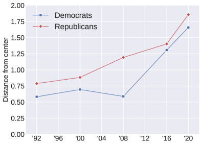
Figure 7: Euclidean distance of the average opinions of Democrats and Republicans from the center, for every year.

It is important to bear in mind that the geometric center only provides information about the average opinion of the group. One can further characterize the opinion of groups by taking into account the heterogeneity of their distribution. If a group populates a large region of the ideological space, their opinions are very heterogeneous, while groups localized within a small region are characterized by more homogeneous opinions. In Fig. 7 of the SM we show the radius of gyration of the opinion distribution of all groups considered, for every year. This magnitude, defined as $R_{g}=\sqrt{\sigma_{x}^{2}+\sigma_{y}^{2}}$, where $\sigma_{x}^{2}$ and $\sigma_{y}^{2}$ are the variances of the coordinates $x$ and $y$ of the embedded opinions, respectively, describes quantitatively how dispersed is the distribution in space, see Materials and Methods. We observe that the opinion dispersion depends more on time than the specific group. The radius of gyration, indeed, clearly increased for all groups in 2016 and particularly in 2020. In general, opinions within a certain group became more heterogeneous over time, with the exception of Black and Republicans, whose opinions remained more homogeneous.

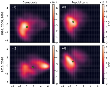
Figure 8: Probability density function (PDF) of Democrats [(a) and (c)] and Republicans [(b) and (d)] in the ideological space. We show the results aggregated over 1992, 2000, and 2008 in (a) and (b), and results over 2016 and 2020 in (c) and (d). The green crosses represent the centroid of each distribution. As in Fig. 1, the axes are arbitrary, combinations of the 29 questions selected.

This last observation indicates that not only has society become much more polarized in the last 10 years, but also the opinions of demographic and political groups have become more heterogeneous. This suggests that ideological polarization could be partially ascribed to minorities departing from the average opinion of their group. Fig. 8 supports this intuition, by showing the opinion distribution of Democrats and Republicans aggregated before 2010 (years 1992, 2000, and 2008) and after 2010 (years 2016 and 2020). One can see that, while the Republican distribution does not change much from the first 20 years to the last 10, the Democrat distribution has become more dispersed in recent years, extending over a large region of the ideological space. Note that the average opinion (centroid) of Democrats in the years 2016 and 2020, represented by a green cross in Fig. 8(c), is poorly representative of the whole distribution, as it falls in the middle of the two most populated areas. Indeed, a group of respondents emerges in a new region of the space (on the right side of the plots), indicating a clear opinion shift in a share of Democratic voters. By comparing their opinions in the two periods, we discovered that the observed shift is mainly due to stronger opinions with respect to affirmative action (particularly regarding Blacks and homosexuals, see SM for details). Therefore, the observed growth in the distance between Democrats and Republicans (shown in Fig. 5) is also due to increasing ideological polarization: A part of Democrats changed their opinions with respect to several issues, moving away from Republican voters. We remark that this opinion change in a part of the population did not lead to an increase in the distance between the average opinions of any demographic group (such as White vs Black), as shown in Fig. 5. Fig. 8 of the SM confirms this intuition, by showing that the respondents occupying the new region of the ideological space are overwhelmingly Democrats (87% Democrats in the new region vs 47% in the general population in 2016 and 2020). Conversely, these respondents show demographic attributes similar to the general population, they are only slightly more educated (College degree: 88% in the new region vs 69% in the general population, High-Income: 43% vs 32%, aged 17-35: 31% vs 23%, Female: 55% vs 53%, Black: 7% vs 9%). Therefore, the observed growth in the partisan divide is due to a combination of partisan sorting and increasing ideological polarization, mainly occurring after 2010.

Conclusions

The ongoing debate about the roots of increasing political polarization revolves around ideological polarization and partisan sorting. While some scientists suggest that ideological polarization has been dramatically increasing over the past several decades Abramowitz and Saunders (2008), others claim instead that Americans sorted themselves into their partisan affiliation Fiorina and Abrams (2008). In this paper, we offer a novel approach to discern between these hypotheses, by embedding the ANES respondents into a two-dimensional ideological space and quantifying their ideological polarization there. First, we confirm that the partisan divide has intensified, especially over the past decade Iyengar et al. (2019); Druckman et al. (2021). The continuous nature of the ideological space allows us to measure the gradient vectors of opinions, discovering that income and racial groups strongly sort into parties. This observation is in line with recent studies Westwood and Peterson (2022), which show that partisanship and race are inseparably linked in American political behavior. However, we also discover that a part of the growing partisan segregation can be attributed to increasing ideological polarization, as quantified by the diverging trajectories of political groups in time. In recent years, indeed, a part of Democratic voters moved into a novel region of the ideological space, closely associated with opinions concerning minority rights. Interestingly, by looking at the voting history of U.S. Congress members, recent research found different trends, i.e., Republicans moved on average further away from the ideological center than Democrats did Desilver (2022). This apparent contradiction can be reconciled by observing that elite polarization does not always go hand-in-hand with mass polarization, especially when the electorate is poorly aware of politics Claassen and Highton (2009).

Our work is not exempted from some limitations. For example, the number of respondents is not the same every year, e.g., it was particularly low in the year 2000. Therefore, we reduced the number of individuals from the more participated surveys, (2016 and 2020), to have a similar number of individuals across years, see Materials and Methods. Likewise, the number of respondents in opposite groups is similar but not equal: Some groups are more populated than their counterparts (see Fig. 3 in the SM). The case of the Race attribute is especially noteworthy, since the majority of ANES respondents are White. Most importantly, we quantify ideological polarization by the distance between average opinions of opposite groups, represented by centroids in the ideological space. This definition might be problematic, since the centroids lose significance for very heterogeneous distributions, such as the one reported in Fig. 8(c). Respondents belonging to the same group could hold substantially different opinions, while the center is located where the density of individuals is almost zero. Similarly, the centroid might be influenced by a few extreme opinions, despite the majority of individuals remaining moderate. To overcome this limitation, we implement measures going beyond simple means Levendusky and Pope (2011); Lelkes (2016), such as the KS distance measuring overlap between distributions, and the radius of gyration gauging heterogeneity. Finally, we remark that our findings are valid within the boundaries of the ANES dataset used, and limited to the questions selected to build the ideological space.

Despite this latter limitation, we believe the novel methodology proposed here can help political and social scientists to better quantify ideological polarization and social sorting. Our framework, indeed, can be applied to any dataset including multiple topics and demographic features of individuals, encompassing a single temporal point or several ones. In this latter case, our approach proved particularly useful, allowing us to chart the trajectories of different demographic and political groups into a single ideological space. In the future, we hope the ANES will continue to collect data regarding the same (or very similar) political, social, and economic topics, to allow tracking of the temporal evolution of these groups. Assembling data sets rich in the temporal dimension is indeed pivotal for a longitudinal assessment of affective polarization among the electorate Phillips (2022). Likewise, with similar data sets it would be possible to gauge more precisely the evolution of social sorting in time. Furthermore, our methods could be applied to countries different from the U.S., where high demographic segregation has been associated with higher levels of affective polarization Harteveld (2021). Interestingly, the increase in partisan divide has also been observed in many countries, while it is not generalizable to all established democracies Garzia et al. (2023). Finally, while our results are purely observational, future work is needed to asses causal connections between ideological polarization, social sorting, and the increase in affective polarization.

Materials and Methods

Here we describe the ANES dataset, the robustness of the dimensionality reduction, and the null model testing the significance of the centroids. Further details can be found in the Supplementary Material (SM).

The ANES dataset

The American National Election Studies (ANES) ane is a continuation of a series of academically-run surveys, asking questions to a representative sample of citizens in the United States about their opinions on all sorts of topics. The 2022 release includes the answers of 68225 respondents throughout a sample of 32 years from 1948 to 2020. The dataset encompasses 1030 variables in total: 161 variables are related to survey information (year, language used, interview mode, etc.) and to information about both interviewer and respondent (gender, race, age, etc.), while the remaining 869 variables consist in the different questions collected by the surveys.

Our objective is to study the ideology of the American population about general topics, thus we narrow down the question list as follows. First, we excluded questions about political parties or election candidates (including presidential candidates). Then, we excluded binary questions (with only two possible answers), which most of the time refer to single events and not general topics, like “Do you read a daily newspaper?”. Since not all the questions have the same number of options to answer, we normalized all the scales to the range $\left[0,1\right]$, with negative and positive extreme answers close to $0$ and $1$, respectively. The ANES dataset is reduced to a total of 99 questions collecting opinions on different topics such as the state of the economy, government spending, religion, or minority rights.

The questions vary over the years, according to the particular socio-economic situation. For example, the disease AIDS was not discovered until the beginning of the eighties, so the question “Should federal spending on AIDS research be increased?” was only included after 1988. To compare the opinions collected throughout different years, we can only take into account shared questions. Since the number of shared questions between pairs of years is maximum after 1990 (see Fig. 1 in the SM), we focus on the last 30 years. Within this time window, we selected the years 1992, 2000, 2008, 2016, and 2020. These years correspond to the election years of the last 5 U.S. Presidents, and are also the ones with the largest number of collected questions. This leaves us with a total of 41 questions. After discarding the ones with a rate of missing answers greater than 20%, the number of shared questions is reduced to 29, which are reported in the SM. Moreover, since the number of respondents in the years 2016 and 2020 is much greater than in 1992, 2000, and 2008, we reduced the former by choosing a random number of respondents, to have a similar number of respondents across years. We checked that this random selection of respondents does not alter our results. In chronological sequence, each year finally contains 2485, 1807, 2322, 2500, and 2500 respondents. This set with 11614 individuals in total forms the final dataset used in the paper.

Dimensionality reduction

To perform the dimensionality reduction of the dataset we apply the Isomap algorithm Tenenbaum et al. (2000). Isomap considers the distribution of the $K$ neighboring data points by attempting to preserve pairwise geodesic (or curvilinear) distances van der Maaten et al. (2009). Isomap estimates the geodesic distance between data points with the shortest path using Dijkstra’s algorithm Dijkstra (1959). The only hyperparameter of the algorithm is then the number $K$ of nearest neighbors. All our findings are obtained by setting $K=10$. Figs. 9-12 in the SM shows that a different choice of the hyperparameter $K$ leads to fully equivalent results. Our Isomap implementation uses manifold from the open-source machine learning library scikit-learn Pedregosa et al. (2011).

Regarding the classification task, we relied on cross-validation for the evaluation of the classification performance, and we used logistic regression as the classification algorithm. As a strategy to split the data into training and testing sets, we used a Stratified K-Fold with 10 splitting iterations. Our computational implementation uses cross_val_score and LogisticRegression from the library scikit-learn Pedregosa et al. (2011).

Furthermore, we tested the robustness of our findings by implementing a different embedding algorithm, the Principal Component Analysis (PCA) Jolliffe (2002). PCA is a linear dimensionality reduction technique, i.e., the new lower dimensions are a linear combination of the original dimensions. In essence, the low-dimensional representation describes as much of the variance in the high-dimensional data as possible. Figs. 13-16 in the SM shows that the PCA embedding leads to similar results. We use PCA from scikit-learn Pedregosa et al. (2011).

Null-hypothesis significance testing

We tested the statistical significance of the average opinions (centroids) of different demographic groups. Our null hypothesis is that opinions do not differ across groups. To test it, we randomly assign each respondent to a demographic group, by preserving the group sizes, $10^{5}$ times for each attribute. If each of the resulting $10^{5}$ centroids is given by the real random vector $\mathbf{X}=\left(X,Y\right)$, we assume that it follows a bivariate normal distribution

$$f\left(\mathbf{x}\right)=\frac{1}{2\pi\sqrt{\left|\Sigma\right|}}\exp{\left[-\frac{1}{2}\left(\mathbf{x}-\mathbf{\mu}\right)\Sigma^{-1}\left(\mathbf{x}-\mathbf{\mu}\right)^{T}\right]},$$ (1)

where $\Sigma$ is the covariance matrix, $\left|\Sigma\right|\equiv\mathrm{det}\left(\Sigma\right)$ and $\mathbf{\mu}=\left(\mu_{x},\mu_{y}\right)$ is the mean vector. The most general form of $\Sigma$ is the symmetric and positive definite matrix

$$\Sigma=\begin{pmatrix}\sigma_{x}^{2}&\rho\sigma_{x}\sigma_{y}\\ \rho\sigma_{x}\sigma_{y}&\sigma_{y}^{2}\end{pmatrix},$$ (2)

where $\sigma_{x},\sigma_{y}$ are the standard deviations of $x$ and $y$, respectively, and $\rho$ is the Pearson correlation coefficient between both coordinates.

By definition, the distance of a point $\mathbf{x}=\left(x,y\right)$ to the bivariate Gaussian given by (1) reads as

$$r\left(\mathbf{x}\right)=\sqrt{\left(\mathbf{x}-\mathbf{\mu}\right)\Sigma^{-1}\left(\mathbf{x}-\mathbf{\mu}\right)^{T}},$$ (3)

which is known as the Mahalanobis distance. If we keep it constant, then the location of $\mathbf{x}$ draws an ellipse centered in $\mu$ with semi-major and semi-minor axes given by the greatest and smallest eigenvalues of $\Sigma$ as $r\sqrt{\lambda_{1}}$ and $r\sqrt{\lambda_{2}}$, respectively Ojer et al. (2022). In a polar coordinate system $\left(r,\theta\right)$, with $r$ given by the Mahalanobis distance defined in (3), a parametric representation of $\mathbf{x}$ can be found as a function of both polar coordinates. Computing analytically the eigenvalues $\lambda_{1}$ and $\lambda_{2}$, we write

$$x = r\sigma_{x}\cos{\left(\theta\right)}+\mu_{x}$$

$$y = r\sigma_{y}\left[\rho\cos{\left(\theta\right)}+\sqrt{1-\rho^{2}}\sin{\left(\theta\right)}\right]+\mu_{y}.$$ (4)

Thus, its Jacobian determinant is $\mathbf{J}_{\mathbf{x}}=r\sigma_{x}\sigma_{y}\sqrt{1-\rho^{2}}=r\sqrt{\left|\Sigma\right|}$.

In the null-hypothesis statistical testing, the p-value is defined as the probability of obtaining results equally or more extreme than the result actually observed, under the assumption that a null-hypothesis is true Fisher (1955). Then, our null hypothesis stands that the observed opinion centroid $\mathbf{x}^{*}$ results from random data distribution, which would mean that it does not give significant information about the system. Following this definition, we compute the p-value corresponding to the observed opinion centroid as

$$p\left(R\right) = \frac{1}{2\pi\sqrt{\left|\Sigma\right|}}\int_{0}^{2\pi}d\theta\int_{R}^{\infty}\mathbf{J}_{\mathbf{x}}\mathrm{e}^{-\frac{r^{2}}{2}}dr$$ (5)

$$= \int_{R}^{\infty}r\mathrm{e}^{-\frac{r^{2}}{2}}dr=\int_{R^{2}/2}^{\infty}\mathrm{e}^{-r}dr=\mathrm{e}^{-R^{2}/2},$$

where $R\equiv r\left(\mathbf{x}^{*}\right)$. As usual, we reject the null-hypothesis if the p-value is less than or equal to the predefined threshold value 0.05 Moore and McCabe (1989).

Heterogeneity of the opinion distribution

Each respondent opinion in the low-dimensional space can be written as a data point $\mathbf{x}=\left(x,y\right)$. How heterogeneous is the distribution of opinions can be computed by means of the covariance matrix given by (2). This square matrix is also known as the radius of gyration tensor, since its greatest and smallest eigenvalues $\lambda_{1}$ and $\lambda_{2}$, respectively, quantify the mean extension of the distribution Rudnick and Gaspari (1987); Ojer et al. (2022). Commonly, therefore, the radius of gyration is used to describe the average dispersion or heterogeneity, and it is defined as $R_{g}=\sqrt{\lambda_{1}+\lambda_{2}}=\sqrt{\mathrm{tr}\left(\Sigma\right)}=\sqrt{\sigma_{x}^{2}+\sigma_{y}^{2}}$.

Charting multidimensional ideological polarization across demographic groups in the United States 
 
Supplementary Material

Jaume Ojer

David Cárcamo

Romualdo Pastor-Satorras

Michele Starnini

Supplementary Material

I ANES dataset

I.1 Preprocessing

In the current release (2022-09-16) of the ANES Cumulative Data File, surveys are performed every 2 to 4 years and conducted in two sessions: before and after presidential elections. Once questions filtered, in Table 2 we collect the number of shared questions for all of the combinations of the ANES editions under consideration: 1992, 2000, 2008, 2016, 2020. We see that if the number of editions increases or they are more distant in time between each other, the number of available questions decreases.

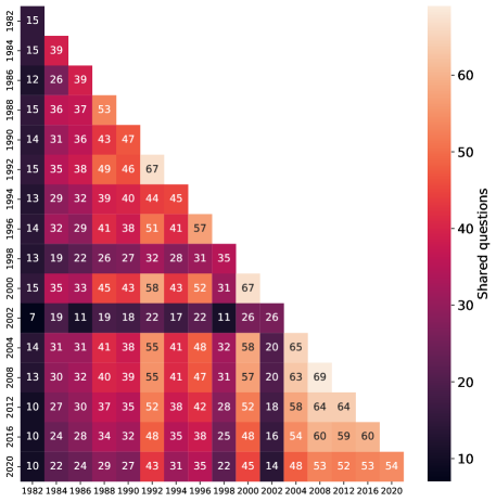
Supplementary Figure SF 1: Number of shared questions between pairs of years for ANES editions after 1980. The main diagonal shows the total number of questions collected in every single year regarding the maximum possible of 99 filtered questions.

Years		Shared questions
(1992, 2000)		58
(1992, 2008)		55
(1992, 2016)		48
(1992, 2020)		43
(2000, 2008)		57
(2000, 2016)		48
(2000, 2020)		45
(2008, 2016)		60
(2008, 2020)		53
(2016, 2020)		53
(1992, 2000, 2008)		52
(1992, 2000, 2016)		45
(1992, 2000, 2020)		41
(1992, 2008, 2016)		48
(1992, 2008, 2020)		43
(1992, 2016, 2020)		43
(2000, 2008, 2016)		48
(2000, 2008, 2020)		44
(2000, 2016, 2020)		44
(2008, 2016, 2020)		53
(1992, 2000, 2008, 2016)		45
(1992, 2000, 2008, 2020)		41
(1992, 2000, 2016, 2020)		41
(1992, 2008, 2016, 2020)		43
(2000, 2008, 2016, 2020)		44
(1992, 2000, 2008, 2016, 2020)		41

Table 2: Number of shared questions available for all of the combinations that result from the ANES editions 1992, 2000, 2008, 2016, 2020.

I.2 Missing data imputation

Missing values in the ANES dataset refer to all the answers to specific questions that are not filled in. This can be due either because no particular opinion is held, or simply because the respondent does not want to answer. Fig. SF 2 shows that for some of the shared questions, the missing rate among the respondents in each ANES edition is high. To work with the most representative samples, we discarded all the questions with a missing rate greater than 20%. The total number of shared questions is then reduced to 29.

Roughly, the underlying mechanism to which the data is missing categorizes it into different classes: missing completely at random (MCAR) or missing not at random (MNAR) Little and Rubin (2002). In the context of opinion surveys, the former refers to the case when the probability of having a missing answer does not depend on either the filled answers or the missing answer itself, whereas the latter refers to the case when the data missingness depends equally on both missing and non-missing data. However, it is mostly impossible to unambiguously categorize missing data into these mechanisms, since finding if missing data is related or not to other non-missing variables can be very challenging Graham (2009). Therefore, the most common alternative is to consider the missing data as missing at random (MAR), i.e., independent of the missing values but related to the filled answers Schafer (1997).

There are different treatment methods intended for handling missing data. One of the simplest approaches is case deletion, which consists of removing all entries with missing values and considering only the remainers. However, this method not only substantially decreases the size of the available dataset, but also introduces bias in data distribution and statistical analysis, especially when missing data is neither MCAR nor MAR. Thus, the most popular process is imputation, which involves replacing missing values with an estimate of the distribution of the non-missing values Little and Rubin (2002); Donders et al. (2006). Simple imputation, for example, replaces missing data by the mean or the median of the available values. However, using constants to replace missing data changes the characteristics of the original dataset, which may produce bias and unrealistic results mostly when dealing with high-dimensional datasets. Another widely used method is regression imputation, which replaces missing data with predicted values created on a regression model. This then assumes that each value depends in some linear way on the other values, although in most cases the relationship is not linear. To achieve the highest possible predictive precision, in this work we impute the missing data through machine learning Emmanuel et al. (2021). In particular, we use the $k$ nearest neighbor ($k$NN) algorithm, by selecting the nearest neighbors of missing values and treating the average value of them as the prediction for imputation. For selecting the $k$ nearest neighbors, the similarity between them and missing data should be maximal, i.e., the Euclidean distance is minimized. Our implementation uses KNNImputer from the open-source machine learning library scikit-learn Pedregosa et al. (2011). The value selection of the hyperparameter $k$ is probably the most sensitive issue when applying the $k$NN algorithm. The substitution of missing data with values that are as close as possible to the true value ceases to be plausible if the data distribution is distorted. Although $k>1$ would in principle lead to better results in terms of imputation precision, 1NN is the only method capable of preserving original data structure  Beretta and Santaniello (2016). For this reason, in this work, we use 1NN to impute all the missing answers.

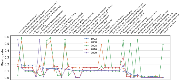
Supplementary Figure SF 2: Rate of missing data for each of the 41 shared questions within the years 1992, 2000, 2008, 2016, and 2020. For our work, we considered the 29 questions with a missing rate lower than 20%.

I.3 Final dataset

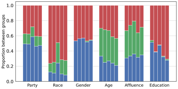
Supplementary Figure SF 3: Proportion of individuals belonging to the different socio-demographic groups of all the attributes considered, over the years (ordered from left to right for each attribute). Following Fig. 2 of the main text, we colored in blue (red) the groups of Democrats, Black, Female, 17-34, Low-Income, and No-College (Republicans, White, Male, 55+, High-Income, and College). We colored in green the remaining groups that were not considered in our work. The total number of individuals is 2485, 1807, 2322, 2500, and 2500 for the years 1992, 2000, 2008, 2016, and 2020, respectively.

Issue	Question	ANES ID
Federal wasted money	Do you think that people in the government waste a lot of money we pay in taxes, waste some of it, or don’t waste very much of it? [A lot, Some, Not very much]	VCF0606
Elections make government pay attention	How much do you feel that having elections makes the government pay attention to what the people think? [Not much, Some, A good deal]	VCF0624
Authority of the Bible	Which of these statements comes closest to describing your feelings about the Bible? [The Bible is the actual Word of God and is to be taken literally, word for word; The Bible is the Word of God but not everything in it should be taken literally, word for word; The Bible is a book written by men and is not the Word of God]	VCF0850
Should adjust view of moral behavior to changes	‘The world is always changing and we should adjust our view of moral behavior to those changes.’ [Agree strongly, Agree somewhat, Neither agree nor disagree, Disagree somewhat, Disagree strongly]	VCF0852
Should be more emphasis on traditional values	‘This country would have many fewer problems if there were more emphasis on traditional family ties.’ [Agree strongly, Agree somewhat, Neither agree nor disagree, Disagree somewhat, Disagree strongly]	VCF0853
Preference on blacks when hiring	Are you for or against preferential hiring and promotion of blacks? [Favor strongly, Favor not strong, Oppose not strong, Oppose strongly]	VCF0867a
Better economy than past year	Would you say that over the past year the nation’s economy has gotten better, stayed the same or gotten worse? [Much better, Somewhat better, Stayed same, Somewhat worse, Much worse]	VCF0871
Protection to homosexuals	Do you favor or oppose laws to protect homosexuals/gays and lesbians against job discrimination? [Favor strongly, Favor not strong, Oppose not strong, Oppose strongly]	VCF0876a
Federal spending: poor people	Should federal spending on aid to poor people be increased, decreased, or kept about the same? [Increased, Same, Decreased or cut out entirely]	VCF0886
Federal spending: dealing with crime	Should federal spending on dealing with crime be increased, decreased, or kept about the same? [Increased, Same, Decreased or cut out entirely]	VCF0888
Federal spending: public schools	Should federal spending on public schools be increased, decreased, or kept about the same? [Increased, Same, Decreased or cut out entirely]	VCF0890
Federal spending: welfare programs	Should federal spending on welfare programs be increased, decreased, or kept about the same? [Increased, Same, Decreased or cut out entirely]	VCF0894
Ensure equal opportunity to succeed	‘Our society should do whatever is necessary to make sure that everyone has an equal opportunity to succeed.’ [Agree strongly, Agree somewhat, Neither agree nor disagree, Disagree somewhat, Disagree strongly]	VCF9013
Life unfair by default	‘It is not really that big a problem if some people have more of a chance in life than others.’ [Agree strongly, Agree somewhat, Neither agree nor disagree, Disagree somewhat, Disagree strongly]	VCF9016
Should worry less about how equal people are	‘This country would be better off if we worried less about how equal people are.’ [Agree strongly, Agree somewhat, Neither agree nor disagree, Disagree somewhat, Disagree strongly]	VCF9017
All should be treated equally	‘If people were treated more equally in this country we would have many fewer problems.’ [Agree strongly, Agree somewhat, Neither agree nor disagree, Disagree somewhat, Disagree strongly]	VCF9018
Blacks have it difficult to succeed	‘Generations of slavery and discrimination have created conditions that make it difficult for blacks to work their way out of the lower class.’ [Agree strongly, Agree somewhat, Neither agree nor disagree, Disagree somewhat, Disagree strongly]	VCF9039

Blacks should not be favored	‘Irish, Italians, Jewish and many other minorities overcame prejudice and worked their way up. Blacks should to the same without any special favors.’ [Agree strongly, Agree somewhat, Neither agree nor disagree, Disagree somewhat, Disagree strongly]	VCF9040
Blacks must try harder	‘It’s really a matter of some people not trying hard enough; if blacks would only try harder they could be just as well off as whites.’ [Agree strongly, Agree somewhat, Neither agree nor disagree, Disagree somewhat, Disagree strongly]	VCF9041
Blacks gotten less than deserved	‘Over the past few years blacks have gotten less than they deserve.’ [Agree strongly, Agree somewhat, Neither agree nor disagree, Disagree somewhat, Disagree strongly]	VCF9042
Federal spending: environment	Should federal spending on improving and protecting the environment be increased, decreased, or stay the same? [Increased, Same, Decreased]	VCF9047
Federal spending: social security	Should federal spending on social security be increased, decreased, or stay the same? [Increased, Same, Decreased]	VCF9049
Presidency and congress splitted	Do you think it is better when one party controls both the presidency and Congress, or when control is split between the Democrats and Republicans? [One party control both, Control is split, It doesn’t matter]	VCF9206
Death penalty	Do you favor or oppose the death penalty for persons convicted of murder? [Favor strongly, Favor not strong, Oppose not strong, Oppose strongly]	VCF9237
Child attribute: curiosity vs good manners	Which one you think is more important for a child to have? [Curiosity, Both, Good manners]	VCF9246
Child attribute: considerate vs well-behaved	Which one you think is more important for a child to have? [Being considerate, Both, Well behaved]	VCF9248
Child attribute: independence vs respect for elders	Which one you think is more important for a child to have? [Independence, Both, Respect for elders]	VCF9249
Hardworking for whites	Where would you rate whites on a scale of 1 to 7? (where 1 indicates hard working, 7 means lazy, and 4 indicates most whites are not closer to one end or the other.) [1. Hard-working - 7. Lazy]	VCF9270
Hardworking for blacks	Where would you rate blacks on a scale of 1 to 7? (where 1 indicates hard working, 7 means lazy, and 4 indicates most blacks are not closer to one end or the other.) [1. Hard-working - 7. Lazy]	VCF9271

Table 3: Overview of all the 29 questions and their respective ANES IDs.

I.4 Opinion shift of Democrats

Table 4 shows the 5 ANES questions with the largest opinion shift by comparing the answers of Democrats of the years 1992, 2000, 2008 with the ones of 2016, 2020 (see Fig. 8 of the main text). Since the amount of Democratic respondents was greater in the first time window than in the second one, we have arbitrarily reduced it in order to work with the same number of individuals in both periods, that is, 2341 Democrats. Taking into account that the answers of respondents range in the numerical interval $\left[0,1\right]$, we calculate the opinion shift before and after 2010 by computing the respective average answers. Therefore, values closer to 0 or 1 represent negative or positive stances, respectively. For example, in the case of “Blacks should not be favored” with the largest shift, the Democratic respondents in (1992, 2000, 2008) agree more strongly than the ones in (2016, 2020). We see that questions are mainly related to minority rights, favoring Blacks and homosexuals, as well as to religion and lifestyle, moving to a more lay and liberal stance.

(1992, 2000, 2008)	(2016, 2020)	Issue
0.656	0.392	Blacks should not be favored
0.558	0.301	Blacks must try harder
0.630	0.400	Authority of the bible
0.681	0.905	Protection to homosexuals
0.749	0.534	Should be more emphasis on traditional values

Table 4: Opinion shift of Democratic respondents between the first 20 years (1992, 2000, 2008) and the last 10 years (2016, 2020). The 5 ANES questions with the largest variation between both periods are shown.

II Supplementary Figures

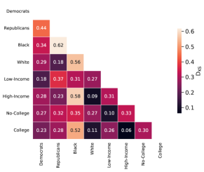
Supplementary Figure SF 4: KS distance $D_{KS}$ between the different socio-demographic groups of the most polarized attributes, aggregated over time. We made the computations by using an updated Python implementation given by the ndtest package syr .

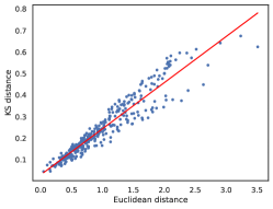
Supplementary Figure SF 5: KS distance as a function of the Euclidean distance between the centroids of all the socio-demographic groups considered. Each point corresponds to one year among 1992, 2000, 2008, 2016, and 2020. The red line represents the linear regression between both distances.

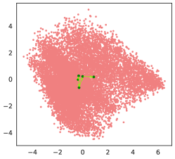
Supplementary Figure SF 6: Two-dimensional ideological space, where each point corresponds to the embedded opinion of each ANES respondent. The average opinions of the different years (1992, 2000, 2008, 2016, 2020) are linked by arrows in chronological sequence.

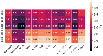
Supplementary Figure SF 7: Radius of gyration $R_{g}$ of the opinion distributions for each group and year.

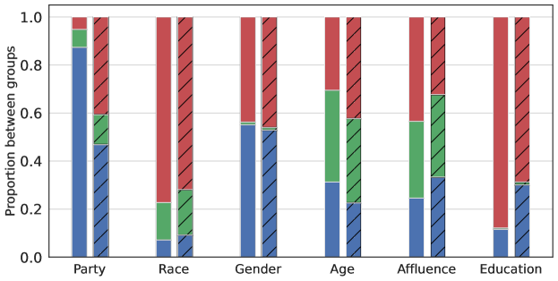
Supplementary Figure SF 8: Proportion of individuals belonging to the different socio-demographic groups of all the attributes considered, by comparing the respondents occupying the new region of the ideological space (solid bars) with the ones aggregated over 2016 and 2020 (hatched bars). Following Fig. 2 of the main text, we colored in blue (red) the groups of Democrats, Black, Female, 17-34, Low-Income, and No-College (Republicans, White, Male, 55+, High-Income, and College). We colored in green the remaining groups that were not considered in our work. The total number of individuals is 1259 in the novel region, and 5000 for the years 2016 and 2020.

II.1 Isomap $K=5$ main results

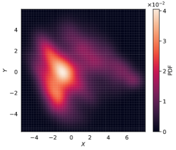
Supplementary Figure SF 9: Probability density function (PDF) of the ANES respondents in the two-dimensional ideological space obtained by Isomap with $K=5$. The lighter (darker) areas are the ones with greater (lower) density. The $X$- and $Y$-axes of the ideological space are arbitrary, combinations of the 29 questions selected.

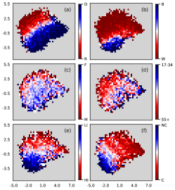
Supplementary Figure SF 10: Density distribution of opposite groups in the ideological space, for different attributes: (a) Democrats (D) and Republicans (R), (b) Black (B) and White (W), (c) Female (F) and Male (M), (d) aged 17-34 and 55+, (e) Low-Income (LI) and High-Income (HI), (f) No-College degree (NC) and College (C). Darker (lighter) cells have a strong (weak) prevalence of one group with respect to the other. Cells with no respondents are colored in gray. We bin the opinion space into 43 $\times$ 39 cells. We slightly smooth data by applying a different Gaussian filter with a low standard deviation for each attribute.

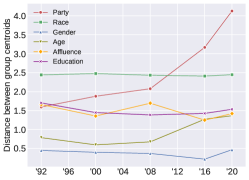
Supplementary Figure SF 11: Euclidean distance between the average opinions (centroids) of the opposite groups of each attribute, for every year.

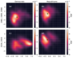
Supplementary Figure SF 12: Probability density function (PDF) of Democrats [(a) and (c)] and Republicans [(b) and (d)] in the ideological space. We show the results aggregated over 1992, 2000, and 2008 in (a) and (b), and results over 2016 and 2020 in (c) and (d). The green crosses represent the centroid of each distribution. The axes are arbitrary, combinations of the 29 questions selected.

II.2 PCA main results

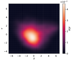
Supplementary Figure SF 13: Probability density function (PDF) of the ANES respondents in the two-dimensional ideological space obtained by PCA. The lighter (darker) areas are the ones with greater (lower) density. The $X$- and $Y$-axes of the ideological space are arbitrary, combinations of the 29 questions selected.

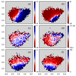
Supplementary Figure SF 14: Density distribution of opposite groups in the ideological space, for different attributes: (a) Democrats (D) and Republicans (R), (b) Black (B) and White (W), (c) Female (F) and Male (M), (d) aged 17-34 and 55+, (e) Low-Income (LI) and High-Income (HI), (f) No-College degree (NC) and College (C). Darker (lighter) cells have a strong (weak) prevalence of one group with respect to the other. Cells with no respondents are colored in gray. We bin the opinion space into 43 $\times$ 36 cells. We slightly smooth data by applying a different Gaussian filter with a low standard deviation for each attribute.

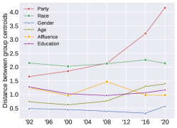
Supplementary Figure SF 15: Euclidean distance between the average opinions (centroids) of the opposite groups of each attribute, for every year.

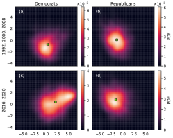
Supplementary Figure SF 16: Probability density function (PDF) of Democrats [(a) and (c)] and Republicans [(b) and (d)] in the ideological space. We show the results aggregated over 1992, 2000, and 2008 in (a) anb (b), and results over 2016 and 2020 in (c) and (d). The green crosses represent the centroid of each distribution. The axes are arbitrary, combinations of the 29 questions selected.