Phase separation of a repulsive two-component Fermi gas at the two- to three-dimensional crossover

Abstract

We present a theoretical analysis of phase separations between two repulsively interacting components in an ultracold fermionic gas, occurring at the dimensional crossover in a harmonic trap with varying aspect ratios. A tailored kinetic energy functional is derived and combined with a density-potential functional approach to develop a framework that is benchmarked with the orbital-based method. We investigate the changes in the density profile of the phase-separated gas under different interaction strengths and geometries. The analysis reveals the existence of small, partially polarized domains in certain parameter regimes, which is similar to the purely two-dimensional limit. However, the density profile is further enriched by a shell structure found in anisotropic traps. We also track the transitions that can be driven by either a change in interaction strength or trap geometry. The developed framework is noted to have applications for other systems with repulsive interactions that combine continuous and discrete degrees of freedom.

I Introduction

Reduced-dimensional systems are of great interest in condensed matter and statistical physics due to the enhanced influence of quantum fluctuations. Such systems are crucial in experimental and technological applications, with examples spanning, e.g., high-temperature superconductors, layered semiconductors, and graphene. Recent advancements in trapping ultracold atomic gases in quasi-two-dimensional geometries [1, 2] have enabled the measurement of zero- [3, 4, 5] and finite-temperature effects [6, 7, 8, 9, 10]. This is usually achieved through strongly anisotropic trapping potentials and one-dimensional optical lattices, which allow for the experimental realization of quasi-two-dimensional quantum gases and dimensional crossovers [11, 12, 13, 14, 15].

Dimensional crossovers provide access to additional degrees of freedom, leading to the emergence of new quantum states with discrete energies. In quasi-two-dimensional Fermi gases, where the transverse confinement energy is comparable to the Fermi energy, the occupation of new transverse states results in a shell structure [11]. This, in turn, causes steps in the density profile, chemical potential, and specific heat to appear as the system size increases due to Pauli exclusion principle [16, 17, 18, 19, 11].

Most of the theoretical and experimental efforts have focused mostly on various many-body effects in two-dimensional Fermi gases, including crossover from Bose-Einstein condensate to Bardeen-Cooper-Schrieffer superfluid [20, 21, 22, 23, 24, 25, 26, 14, 27], or pairing pseudogap [28, 29, 10, 30]. As in realistic experimental scenarios, the anisotropy of confining potentials does not usually allow for purely two-dimensional regime, the analysis of dimensional crossovers has been of particular interest [11, 12, 13, 31, 32, 14, 5, 33, 34, 15, 35]. Such transitions happen close to the ground state of the considered system and manifest the underlying bonding mechanism in a Fermi gas.

However, when excited, the spin components of a Fermi gas, i.e., given by two chosen hyperfine states, may exhibit repulsive correlations, being brought to the so-called repulsive branch. In the case of a gas trapped in a harmonic potential, that repulsion may lead to a metastable phase separation between the components, an ultracold analog of celebrated Stoner instability in Coulomb-interacting electronic gas [36]. Experimentally elusive in both three and two dimensions due to the eventual decay to the ground state, this itinerant ferromagnetic state has been widely researched both theoretically [37, 38, 39, 40, 41, 42, 43, 44, 45, 46, 47, 48, 49, 50, 51, 52, 51, 53, 54, 55, 56, 57, 58, 59, 60] and experimentally [61, 62, 63, 64, 65, 66, 67, 68, 69, 70, 71], also in different mixtures [72, 73, 74].

We focus on previously unexplored crossover of the Stoner instability between two and three dimensions, analyzing the purely repulsive system of two fermionic components trapped in an anisotropic trap with varying aspect ratio and interaction strength. In the three-dimensional limit, the repulsive gas in a radially symmetric trap exhibits both partially and fully polarized phases, whose density profiles remain highly regular, either in a ring structure, with one of the components dominating in the center of the trap, or in two halves separated by a single domain wall [49]. In contrast, in two dimensions, contact-interacting gas can form a plethora of partially polarized states manifesting many small domains, due to a lack of scaling of critical interaction strength with respect to the density of gas in the leading order [57]. In each of these cases, refined treatment of the kinetic energy, going beyond the usual Thomas-Fermi approach, is necessary, as the competition between the kinetic, interaction, and correlation energy drives the exact shape of the density profile.

To take that into account and to describe systems of sizes reaching usual experimental scenarios of large Fermi clouds, we utilize orbital-free density-potential functional theory (DPFT) that was proven to accurately determine the complex phases of interacting Fermi gases [75, 76, 77, 78, 79, 80, 81, 82, 83]. It achieves this by simplifying the many-body problem to two self-consistent equations: one for the single-particle density and another for an effective potential that accounts for the interactions. DPFT is particularly useful for simulating trapped quantum gases, especially in two-dimensional configurations. Conventional density-functional theory (DFT) techniques are unable to match DPFT’s capabilities in this regard, as they are either limited to small particle numbers [84, 85], periodic confinement [86], or rely on ad-hoc parameterizations of the kinetic energy [87, 88]. Although systematic gradient corrections in two dimensions are available for electronic systems [89], DPFT offers a scalable approach that can be systematically expanded beyond the Thomas-Fermi approximation across one-, two-, and three-dimensional geometries.

In this work we examine phase transitions from para- to ferromagnetic states in a binary Fermi gas, involving two- to three-dimensional crossover using density-potential functional theory and Hartree-Fock methods. To this end, we derive a tailored kinetic energy functional for a dimensional crossover of the Fermi gas and combine it with the density–potential functional approach to allow the description of large particle numbers. We use the Hartree-Fock method to benchmark our results in the low-atom-number limit. Our findings indicate highly degenerate ground-state profiles during the transition, featuring various shapes like isotropic and anisotropic separations, ring-shaped polarization, and central splits within a shell structure. These profiles can be manipulated by adjusting particle number, interaction strength, and trapping aspect ratio, offering a versatile exploration of interacting quantum mixtures.

The paper is structured as follows. Section II outlines the derivations of the kinetic and interaction energy functionals for the dimensional crossover, with specific details placed in Appendices A and B, along with the presentation of the DPFT and Hartree-Fock methods. Section III provides a description of the results we have obtained, including interaction- and aspect-ratio-driven phase transitions, comparison between two methods, and analysis of large-particle-number limit. We conclude the paper in Section IV, providing a summary and outlook for the future.

II Methods

II.1 Density functional approach for a Fermi gas at a two- to three-dimensional crossover

We derive the Thomas-Fermi kinetic energy expression for a two-dimensional (2D) noninteracting, zero-temperature, uniformly polarized Fermi gas of mass $m$ with an extra degree of freedom tied to successive energy states of a harmonic oscillator. This analysis captures a Fermi gas confined perpendicularly by a harmonic potential, creating a quasi-2D scenario. In strong confinement, when perpendicular excitation energy $\hbar\omega$ greatly exceeds Fermi energy $E_{F}$ an exact 2D description emerges. We explore cases where $E_{F}$ slightly surpasses $\hbar\omega$ without violating the assumption of low perpendicular density of states. Within this assumption, we obtain the following kinetic energy functional (the detailed calculation is provided in App. A):

$$\epsilon_{K}[n]=\frac{\pi\hbar^{2}}{(l+1)m}n^{2}+\frac{m\omega^{2}}{48\pi}l(l+1)(l+2),$$ (1)

where $l$ has to be self-consistently calculated as

$$\left\lfloor{\frac{2\pi\hbar^{2}}{(l+1)m\hbar\omega}n+\frac{1}{2}l}\right\rfloor=l.$$ (2)

The full energy functional, including the perpendicular degree of freedom yields:

$$\epsilon[n]=\frac{\pi\hbar^{2}}{(l+1)m}n^{2}+\frac{1}{2}l\hbar\omega n-\frac{l(l+1)(l+2)m\omega^{2}}{48\pi}.$$ (3)

The functional derivative of the functional is then:

$$\frac{\delta}{\delta n(\mathbf{r})}\int\text{d}\mathbf{r}\,\epsilon[n(\mathbf{r})]=\frac{2\pi\hbar^{2}}{(l+1)m}n(\mathbf{r})+\frac{l\hbar\omega}{2},$$ (4)

where dependence on spatial coordinate $\mathbf{r}=(x,y)$ signifies nonuniform density profile $n(\mathbf{r})$. As a next step, we introduce the Ansatz for three-dimensional density,

$$\widetilde{n}_{3D}(n_{2D},z)=\frac{m}{2\pi\hbar^{2}}\times$$

$$\sum_{j=0}^{l}\left\{\frac{1}{l+1}\left(\frac{2\pi\hbar^{2}}{m}n_{2D}+\frac{1}{2}\hbar\omega l\left(l+1\right)\right)-j\hbar\omega\right\}n_{j}(z),$$ (5)

whose derivation can be found in App. A. Here,

$$n_{j}(z)=\frac{1}{2^{j}j!}\sqrt{\frac{m\omega}{\pi\hbar}}e^{-\frac{m\omega z^{2}}{\hbar}}H_{j}^{2}\left(\sqrt{\frac{m\omega}{\hbar}}z\right),$$ (6)

where $H_{j}$ is j${}^{\text{th}}$ Hermite’s polynomial.

Let us now consider a binary mixture of two spin-polarized Fermi gases with densities $n_{1}$ and $n_{2}$ and define the total contact interaction energy as

$$E_{\text{int}}=g\int n_{1}(\bm{r})\ n_{2}(\bm{r})\ \differential\bm{r},$$ (7)

where $g$ is a three-dimensional coupling constant. Then, if we define two-dimensional interaction energy functional $\epsilon_{\text{int}}[n_{1}(x,y),n_{2}(x,y)]$ as

$$E_{\text{int}}=\int\epsilon_{\text{int}}[n_{1}(x,y),n_{2}(x,y)]\differential x\differential y,$$ (8)

we can simplify it to

$$\epsilon_{\text{int}}[n_{1}(x,y),n_{2}(x,y)]=$$

$$g\sqrt{\frac{m\omega}{\hbar}}n_{1}n_{2}\eta_{1}(l_{1},l_{2})+g\sqrt{\frac{m\omega}{\hbar}}\frac{m\omega}{2\pi\hbar}n_{1}\eta_{2}(l_{1},l_{2})+$$

$$g\sqrt{\frac{m\omega}{\hbar}}\frac{m\omega}{2\pi\hbar}n_{2}\eta_{2}(l_{2},l_{1})+g\sqrt{\frac{m\omega}{\hbar}}\frac{m^{2}\omega^{2}}{4\pi^{2}\hbar^{2}}\eta_{3}(l_{1},l_{2}),$$ (9)

where exact forms of functions $\eta_{i}$ are given in App. B. With these formulas, we are equipped to construct a density–potential functional theory framework for the dimensional crossover of a Fermi gas.

II.2 Density–potential functional theory

The exact DFT energy functional can be rephrased as a bifunctional of the densities $\mathbold{n}$ (here, ${\mathbold{n}=\{n_{s}\}=(n_{1},n_{2})}$ for fermion species ${s=1,2}$) and effective potential energies $\{V_{s}\}$ that combine the interaction effects with the external potential energies $V_{s}^{\mathrm{ext}}$ [80, 81, 90, 91, 57, 92, 93, 94, 95]. We find the ground-state densities $n_{1}$ and $n_{2}$ among the stationary points of this bifunctional by self-consistently solving

$$n_{s}[V_{s}-\mu_{s}](\mathbold{r})=\frac{\delta E_{1}[V_{s}-\mu_{s}]}{\delta V_{s}(\mathbold{r})}$$ (10)

and

$$V_{s}[\mathbold{n}](\mathbold{r})=V_{s}^{\mathrm{ext}}(\mathbold{r})+\frac{\delta E_{\mathrm{int}}[\mathbold{n}]}{\delta n_{s}(\mathbold{r})}\,.$$ (11)

Here, $E_{1}[V_{s}-\mu_{s}]$ is the Legendre transform of the kinetic energy functional $E_{\mathrm{kin}}[n_{s}]$, $\mu_{s}$ is the chemical potential for species $s$, and the interaction energy $E_{\mathrm{int}}[\mathbold{n}]$ generally couples all densities. For the general formalism and many applications of this density–potential functional theory (DPFT) we refer to [80, 81, 90, 91, 57, 92, 93, 94, 95] and references therein. In particular, we will deploy the exact same machinery for two-component interacting fermion gases as in [57], with the twist of transferring the kinetic energy contribution that stems from the transversal direction to the interaction energy. This augmentation of the DPFT framework allows us to predict the properties of 3D systems at the cost of 2D calculations.

Specifically, by adding and subtracting the TF kinetic energy density ${\epsilon^{\mathrm{TF,2D}}_{\mathrm{kin}}=\pi n^{2}}$ (in harmonic oscillator units) for spin-polarized fermions in 2D, we write the full energy density (3) as

$$\epsilon[n]=\epsilon^{\mathrm{TF,2D}}_{\mathrm{kin}}+\epsilon^{\mathrm{2D3D}}_{\mathrm{int}}\,.$$ (12)

Here, the effective interaction energy density

$$\epsilon^{\mathrm{2D3D}}_{\mathrm{int}}=\left(\frac{\pi}{l+1}-\pi\right)n^{2}+\frac{1}{2}l\,n\,\omega-\frac{\omega^{2}}{48\pi}l(l+1)(l+2)$$ (13)

compensates for the introduction of the 2D TF kinetic energy in (12). Since $l(n)$ is piecewise constant, the functional derivative of the energy ${E^{\mathrm{2D3D}}_{\mathrm{int}}[n]=\int\mathrm{d}\mathbold{r}\,\epsilon^{\mathrm{2D3D}}_{\mathrm{int}}}$ is

$$\frac{\delta E^{\mathrm{2D3D}}_{\mathrm{int}}[n]}{\delta n(\mathbold{r})}=\frac{-2\pi\,n(\mathbold{r})\,l}{l+1}+\frac{\omega\,l}{2},$$ (14)

which we incorporate into the effective interaction potential in (11), such that we can execute the self-consistent program of (10) and (11) in a pure 2D setting.

Finally, we may replace the quasi-classical TF kinetic energy $E^{\mathrm{TF,2D}}_{\mathrm{kin}}$ by semiclassical approximations of the (Legendre-transformed) kinetic energy functional, viz., approximations of $E_{1}[V-\mu]$; all details of the numerical procedures are discussed in [57]. Accordingly, we deploy the nonlocal quantum-corrected successor

$$n_{3^{\prime}}(\mathbold{r})=g\int(\mathrm{d}\mathbold{r}^{\prime})\left(\frac{k_{3^{\prime}}}{2\pi r^{\prime}}\right)^{D}J_{D}(2r^{\prime}\,k_{3^{\prime}})$$ (15)

of the local TF density for $D$ dimensions, see [82, 57], with the Bessel function $J_{D}(\,)$ of order $D$ and the effective Fermi wave number

$$k_{3^{\prime}}=\frac{1}{\hbar}\big{[}2m\big{(}\mu-V(\mathbold{r}+\mathbold{r}^{\prime})\big{)}\big{]}_{+}^{1/2},$$ (16)

where ${[z]_{+}=z\,\Theta(z)}$, and $\Theta(\,)$ is the Heaviside step function.

II.3 Orbital approach

We benchmark $n_{3^{\prime}}$-based DPFT densities against Hartree–Fock (HF) results. In this work, we use time-dependent HF equations

$$i\hbar\frac{\partial}{\partial t}\varphi_{i}^{(s)}({\mathbold{r}},t)=\left[-\frac{\hbar^{2}}{2m}\nabla^{2}+V_{ext}({\mathbold{r}},t)\right.$$

$$+\left.\frac{\delta E_{\text{int}}[\mathbold{n}]}{\delta n_{s}(\mathbold{r},t)}\;\right]\;\varphi_{i}^{(s)}({\mathbold{r}},t)$$ (17)

for the two-component spin mixture (${s\in\{1,2\}}$). The derivation of these equations is shown in App. C. Here, $\varphi_{i}^{(1)}(\mathbold{r},t)$ and $\varphi_{i}^{(2)}(\mathbold{r},t)$, with ${i=1,...,N/2}$, are spatial orbitals of the first and the second spin component, respectively. The interaction terms $\frac{\delta E_{\text{int}}[\mathbold{n}]}{\delta n_{1/2}(\mathbold{r},t)}$ are defined below through equation (7). The one-particle densities

$$n_{s}(\mathbold{r},t) = \sum_{i=1}^{N/2}|\varphi_{i}^{(s)}(\mathbold{r},t)|^{2}$$ (18)

associated with the spin components $s$ sum to the total one-particle density $n(\mathbold{r},t)=n_{1}(\mathbold{r},t)+n_{2}(\mathbold{r},t)$.

We are looking for the ground-state densities. We are solving the set of equations (II.3) by the imaginary time propagation technique [96] where real time is replaced by imaginary time $t\rightarrow-i\tau$. After that, the evolution operator is no longer a unitary operator. Both the norm and the orthogonality are lost during the imaginary time propagation. To keep the orthogonality and the norm of the spatial orbitals we use the Gram-Schmidt orthonormalization technique. This way, propagating $N$ spatial orbitals we obtain the ground state of $N$ particles.

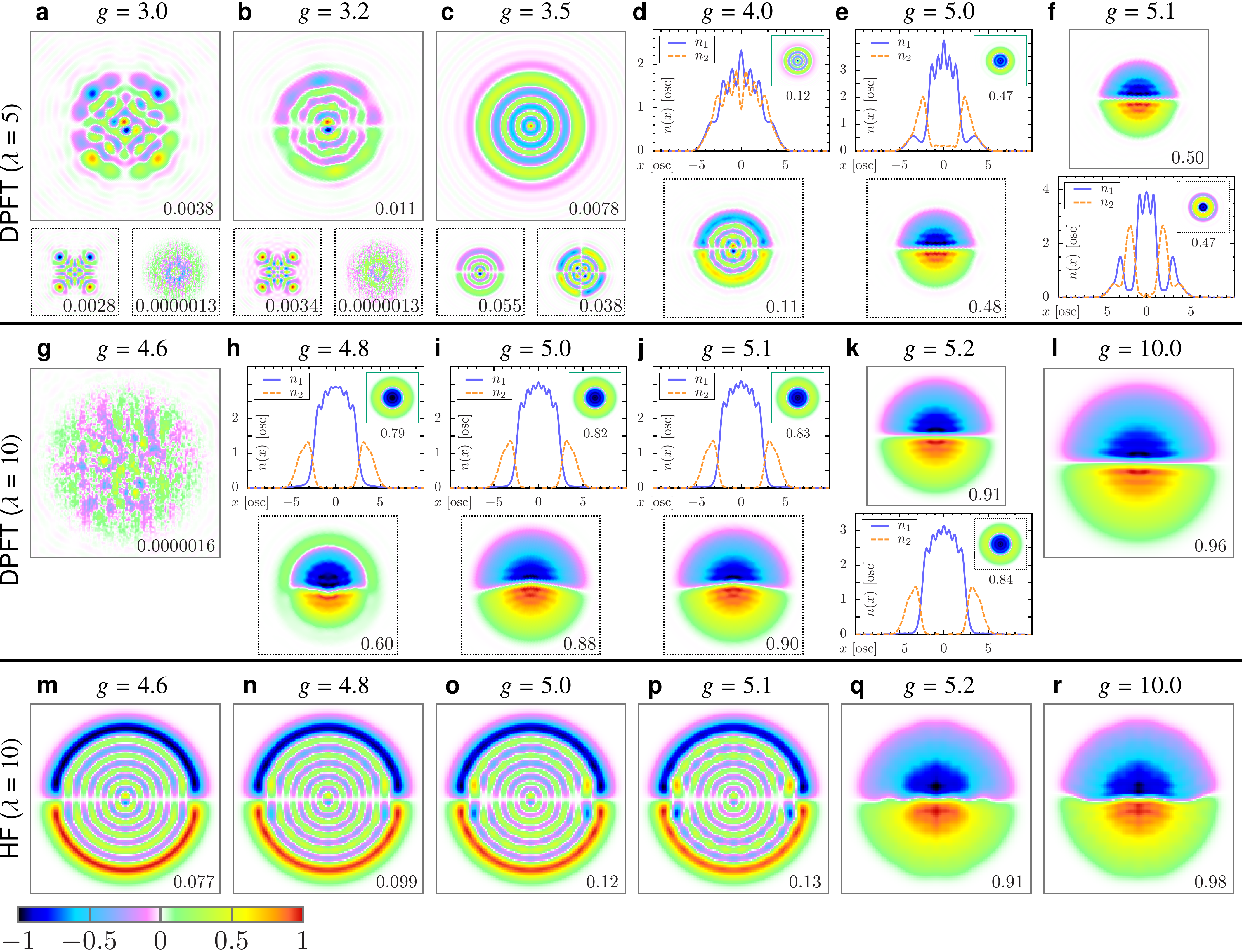
Figure 1: The density profiles for a two-component repulsive Fermi gas across interaction-driven phase transitions. The top (bottom) plots in each panel present the ground-state (metastable, closely matched in energy) profiles. The density profiles are plotted either as density differences $n_{1}-n_{2}$, scaled by $\mathrm{max}_{\mathbold{r}}|n_{1}(\mathbold{r})-n_{2}(\mathbold{r})|$, which are presented as contour plots in a square box with edge lengths of 6 [osc] (the color legend applies to all the contour plots); or as density cross-sections at ${y=0}$. (a-f) Ground-state density profiles for a fixed aspect ratio of the harmonic trap ($\lambda=5$) and a constant total number of particles ($N_{1}=N_{2}=55$). These profiles vary with the three-dimensional repulsive coupling constant between the two species, denoted as $g$, and are characterized through a global polarization $\mathcal{P}$. Notably, two distinct phase transitions are observable: one from a paramagnetic to an isotropic, partially polarized phase, followed by a transition to a two-hemisphere state. The findings are obtained using a density-potential functional approach. (g-l) Similarly presented are ground-state density profiles for a higher aspect ratio of the trap ($\lambda=10$). (m-r) The results in this row are analogous to those in the second row; however, they are computed using the Hartree-Fock approach. Although the weak- and large-interaction limits yield comparable outcomes, disparities become evident within the phase transition regime. See Table 1 for details of each panel, including interaction strength, scaling factor, energy, polarization, and transverse excitations.

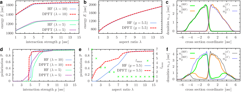
Figure 2: (a,b) Total energy of a two-component Fermi gas throughout interaction and aspect ratio sweeps for two methods—density–potential functional theory and Hartree-Fock. Both methods show similar predictions. (d,e) The same but for the total polarization. In this case, the two methods match for strong interactions and high aspect ratios, but otherwise yield density profiles with quite different polarizations—a sign of near-degenerate states across the transitions w.r.t. $g$ and $\lambda$. (c,f) Comparison of density cross-section for both methods. The slopes of the densities match very well for strongly interacting clouds.

III Results

Our focus lies predominantly on analyzing phase transitions in a binary Fermi gas, dependent on three key physical parameters: the number of particles, the aspect ratio, and the strength of three-dimensional interactions. These transitions manifest as distinct phase transitions in the ground-state densities of the gas components. Past research has highlighted that in radially symmetric harmonic trapping, transitions occur from uniform density profiles of the two fermion species to both isotropic and anisotropic separations. Furthermore, within a purely two-dimensional configuration with bare contact interaction, an analogous transition arises [57]. This transition shifts from a paramagnetic state at low repulsive interactions to ferromagnetic density profiles at higher interaction strengths. However, intricate particle-number-dependent phases emerge between these limits. Moreover, a range of metastable configurations with energy levels comparable to ground-state density profiles have been identified within the transitional regime. These configurations are likely to be observed in experimental settings. Hence, our analysis seeks to uncover the crossover between these two scenarios, achievable by transitioning dimensionally through adjustments in the trap’s aspect ratio. For the analysis of spatial separation at the crossover, we will utilize a total polarization $\mathcal{P}$ of the trapped mixture:

$$\mathcal{P}=\frac{\int\mathrm{d}\mathbf{r}\left|n_{1}(\mathbf{r})-n_{2}(\mathbf{r})\right|}{N}.$$ (19)

III.1 Interaction-driven phase transitions

We begin by examining a specific scenario where we vary interaction strengths while keeping the aspect ratio $\lambda=5$ and particle count $N_{1}=N_{2}=55$ constant. We present it in Fig 1(a-f). At low interaction strengths, a paramagnetic phase is observed, where nearly identical density profiles with accordingly small energy differences make it difficult to distinguish the ground state from metastable states. Although overall polarization remains low as we increase the interaction strength to around $g=3.5$, slight polarization modulations emerge near the center due to a relative decrease in interaction energy at the expense of kinetic energy. At ${g=3.5}$ this trade-off between the energy components begins to favor ground-state profiles with isotropic separations. This transition is characterized by visible domains without breaking radial symmetry. We identify states in close energy proximity that break radial symmetry and possess nonzero polarization. These states bear a resemblance to findings in purely 2D scenarios. Further along, as the interaction strength reaches $g=5$, the gas segregates into two hemispheres, mirroring the analogous behavior observed in both 2D and 3D.

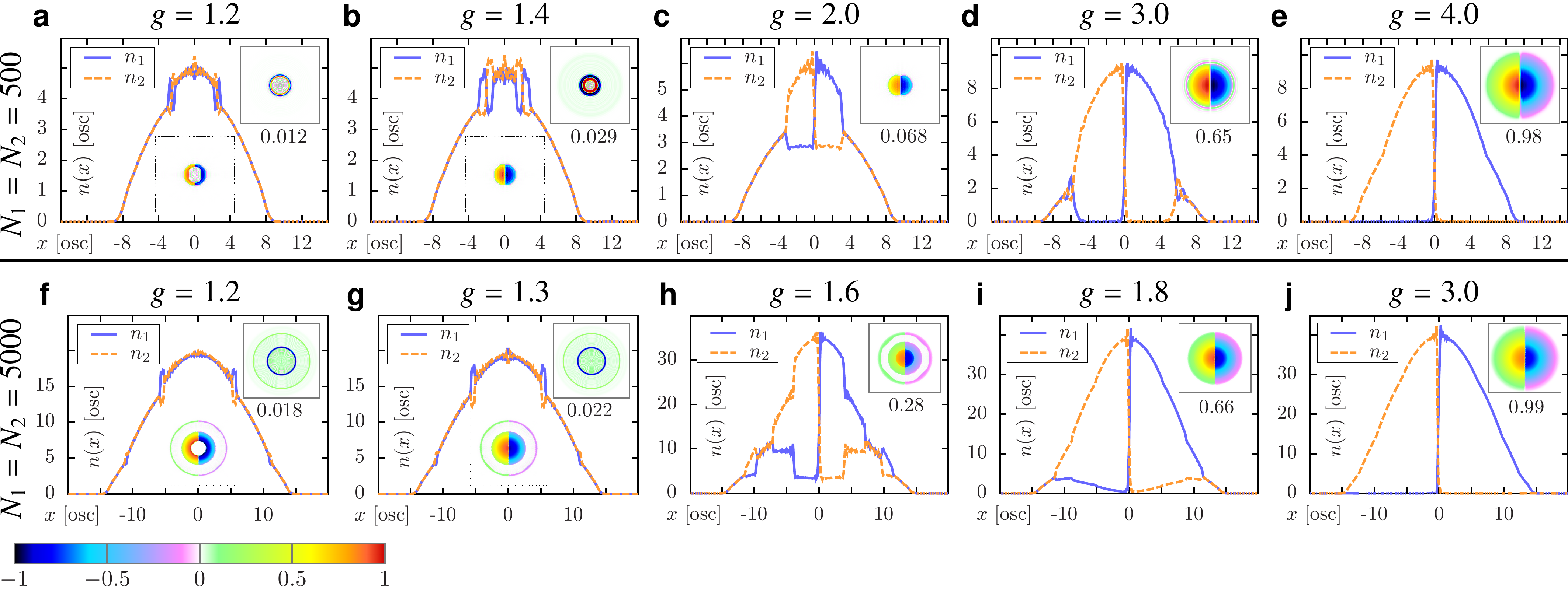
Figure 3: (a-e) Ground-state density profiles for a two-component repulsive Fermi gas, with a fixed aspect ratio of the harmonic trap ($\lambda=25$) and a constant total number of particles ($N_{1}=N_{2}=500$). These profiles vary with the three-dimensional repulsive coupling constant between the two species, denoted as $g$. Richer density profile structure across the para- to ferromagnetic phase transition is visible, as compared to the lower atom number case, exhibiting ring-shaped polarization and central-split patterns. (f-j) The same but for $\lambda=30$ and $N_{1}=N_{2}=5000$. The density profile gets even more intricate, showing the coexistence of ring-shaped polarization and central-split patterns for some values of interaction strength. The main plot and the top right inset in each panel present the ground-state profiles. In panels a, b, f, and g, we also show metastable profiles. The density differences $n_{1}-n_{2}$, scaled by ${\mathrm{max}}_{\mathbold{r}}|n_{1}(\mathbold{r})-n_{2}(\mathbold{r})|$, are presented as contour plots in a square box with edge lengths of 10 [osc] (15 [osc]) for $N_{1/2}=500$ ($N_{1/2}=5000$); the color legend applies to all the contour plots. See Table 2 for details.

Subsequently, we compare these results with those from an altered aspect ratio, $\lambda=10$ [refer to Fig. 1(g-l)]. We observe analogous behavior; however, the initial transition from no separation to isotropic separation is more pronounced, lacking an easily distinguishable transitional regime characterized by minor polarization modulations. This transition occurs at $g=4.65$ and is followed by a mirror-symmetric separation at ${g=5.15}$ that grows into an almost complete split separation at ${g=10}$. Again, we find metastable states across the transitions, which show competition between different types of splittings. However, for this particular aspect ratio and atom number, the competition is mainly between isotropic and anisotropic separation states.

These findings are consistent with both two- and three-dimensional cases; however, they indicate that the fine structure of coexisting metastable states strongly depends on the perpendicular excitation structure. Symmetry-breaking partially polarized profiles are unveiled for lower aspect ratios when the perpendicular degree of freedom is more intensely excited, in contrast to the higher aspect ratio case where such structures are not easily discernible, cf. Table 1. This showcases nontrivial behavior, similar to the scenario in the limit of pure two-dimensional geometry where these metastable states are present.

III.2 Benchmarking DPFT against Hartree–Fock

We now move on to validate the previously described low-atom-number outcomes using the orbital approach. We compare density profiles throughout the interaction-induced phase transition for $\lambda=10$ and $N_{1}=N_{2}=55$, as displayed in Fig 1(m-r). While we observe that within the weak interaction limit, the paramagnetic, identical density profiles of both clouds are consistent across both methods, a slight discrepancy emerges at the onset of the phase transition. The isotropic transition is not evident, but instead, the ground state just above the transition assumes a partially polarized, symmetry-breaking configuration. It’s worth noting that the density structure of this state bears a resemblance to certain profiles of metastable states identified using the DPFT method. This observation suggests that the ground state at the transition is nearly degenerate, with various density profiles being realized by states with minute energy differences. We hypothesize that the divergence between the methods regarding the true ground state arises from the proximity of these states. Importantly, in Hartree-Fock calculations, the subsequent phase transition to a two-hemisphere state occurs at a similar value of the interaction strength as observed in the DPFT method. In the scenario of a large interaction limit, density profiles between the two methods align remarkably well.

To conduct a more comprehensive analysis of this comparison, we present in Fig. 2 the comparison between the two methods across both interaction and aspect ratio variations. We employ total energy and total polarization as metrics for assessment. First, we find that energies match very well across both transitions, suggesting consistency between both methods. As for the total polarization, the behavior across the transition is qualitatively captured with a good quantitative match in the strong coupling regime. This slight quantitative mismatch suggests that the total polarization is a sensitive probe for specifying which state is realized experimentally. Importantly, comparing the cuts through the density profiles, we find that the slopes of the density profiles match in both methods, implying a mutually consistent description of the interplay of kinetic and interaction energies in both methods. Such a behavior is of particular interest as domain-wall density profile determines, e.g., dimer formation rates in ultracold gases.

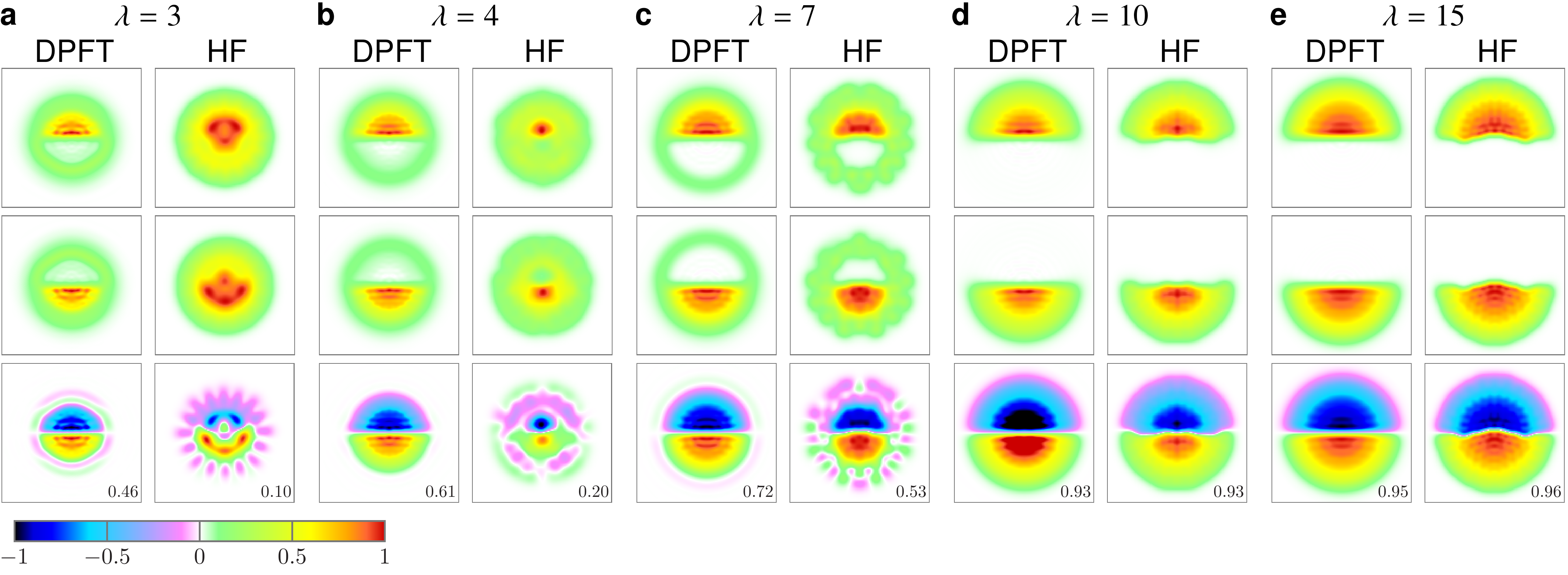
Figure 4: Ground-state density profiles for a two-component repulsive Fermi gas, with a fixed coupling constant between two fermionic components ($g=5.5$) and a constant total number of particles ($N_{1}=N_{2}=55$). These profiles vary with the aspect ratio of the harmonic trap $\lambda$, exhibiting a transition from partially to fully polarized state. The top (bottom) plots in each panel present the ground-state (metastable) profiles. The density differences $n_{1}-n_{2}$, scaled by ${\mathrm{max}}_{\mathbold{r}}|n_{1}(\mathbold{r})-n_{2}(\mathbold{r})|$, are presented as contour plots in a square box with edge lengths of 6 [osc]; the color legend applies to all the contour plots. See Table 3 for details.

III.3 Large-atom-number limit

We now proceed to analyze large atom number setups that go beyond the manageability of the Hartree-Fock approach due to numerical cost. In Fig. 3 we present two cases, $N_{1}=N_{2}=500$ and $N_{1}=N_{2}=5000$, both computed with DPFT approach. In these cases, the shell structure of the density profiles, usual in low-dimensional experimental setups, i.e., sharp transitions in the densities due to discretized energy spectrum in transversal direction, becomes apparent. First, we observe that the existence of these sharp density changes makes the competition between kinetic and interaction energy even more intricate. As we go through the interaction-induced transition for $N_{1}=N_{2}=500$, we find that partial polarization may be favored at these density changes, revealing a ring-shaped polarization pattern that might or might not preserve radial symmetry. As the interaction strength increases above ${g\approx 1.4}$, the preferred density profile involves the anisotropic split at the center of the trap and a shell structure at the perimeter. With the further growing interaction, this central split occupies more volume, becoming two fully separated hemispheres in the strong interaction regime. Notably, in this case, no ground-state isotropic separation is observed. The $N_{1}=N_{2}=5000$ case exhibits similar behavior. Across the phase transition toward a ferromagnetic state, one observes the coexistence of both isotropic and anisotropic ring-shaped polarization structures and the central anisotropic split, shown in the lower atom number case.

III.4 Geometry-driven transitions

Up to now, we have analyzed a phase transition driven by the varying interaction. Here, we would like to focus on the case in which the ground-state density profile is altered through the change of geometry via the aspect ratio of the harmonic trap. In Fig. 4 we plot the transition for $g=5.5$ and $N_{1}=N_{2}=55$, while the aspect ratio is changed from $\lambda=3$ to $\lambda=15$ [compare Fig. 2(e), where total polarization is plotted for this transition]. Such a sweep realizes a transition from a partially polarized anisotropic split to the fully separated hemispheres. In the limiting cases, the phase separation occurs at $g\approx 7$ for $\lambda=1$ the [49] and at $g\approx 15.7/\sqrt{\lambda}$ for the two-dimensional limit $\lambda\rightarrow\infty$ [57] (which equals $g=5.0$ and $g=4.1$ for $\lambda=10$ and $\lambda=15$, respectively). It shows how the geometry can be used to drive the phase transition, similarly to experiment with, e.g., confinement-induced resonances [97].

IV Conclusions and outlook

Summarizing, we have analyzed para- to ferromagnetic phase transition in a binary repulsive Fermi gas at a two- to three-dimensional crossover utilizing two distinctive methods—density–potential functional theory and Hartree-Fock methods. We have found out that in a quasi-two-dimensional regime, the ground-state profile across the phase transition is nearly degenerate and exhibits a variety of shapes, including isotropic and anisotropic separations, ring-shaped polarization patterns, and central-split patterns in the usual shell structure. These density profiles can be tuned via means of varying particle number, interaction strength, and aspect ratio of the external trapping, providing a versatile playground for the physics of interacting quantum mixtures. As these various density profiles stem from an intricate interplay between kinetic, potential, and interaction energy, as a direction for future analysis one may include quantum corrections to the mean-field treatment of the interaction energy and allow for nonzero temperature that would smear out fine density features in more realistic experimental scenarios. As a concluding remark, it’s worth noting that the multiparticle Hamiltonian governing the system in this paper exhibits axial symmetry. This implies that, unless degenerate, the ground state must also possess axial symmetry. However, the observed symmetry-breaking single-particle patterns, detailed in this study, are entirely physical as they accurately describe individual experimental shots. This somewhat paradoxical aspect of the density functional method was recently highlighted in [98].

V Acknowledgements

The Center for Theoretical Physics of the Polish Academy of Sciences is a member of the National Laboratory of Atomic, Molecular and Optical Physics (KL FAMO). This work has been supported by the National Research Foundation, Singapore and A*STAR under its CQT Bridging Grant and its Quantum Engineering Programme. Part of the results were obtained using computers of the Computer Center of the University of Białystok.

Appendix A Derivation of a kinetic energy functional

We derive an expression for Thomas-Fermi kinetic energy functional for two-dimensional noninteracting zero-temperature uniform polarized Fermi gas under the assumption that it has another degree of freedom, as it can occupy consecutive energy states of the harmonic oscillator. The aim of this treatment is to describe a Fermi gas that is strongly confined in one direction (perpendicular) by a harmonic potential, namely in the quasi-2D situation. In the limit of very strong confinement, when the energy of excitation in the perpendicular direction $\hbar\omega$ is much higher than the Fermi energy of the gas $E_{F}$, we retrieve a description that is exactly two-dimensional. We consider the situation in which we allow the Fermi energy to exceed the perpendicular excitation energy but not too much in order not to destroy the assumption of the low density of states in the perpendicular direction.

We start with a semi-classical picture of two-dimensional Fermi gas. To calculate kinetic energy functional we first assume that consecutive fermions occupy consecutive energy levels described by two quantum numbers, $k_{x}$ and $k_{y}$, up to Fermi energy. We integrate over the $k$-space, effectively calculating the volume of a 2D sphere of radius $k_{F}$. We then assume that every state resides in $1/(2\pi/L)^{2}$ fraction of the sphere’s volume and this way we get the number of all particles $N$ and following that, the density of particles, $n=N/L^{2}$. Then we similarly calculate the expectation value of the kinetic energy, $\frac{\hbar^{2}k^{2}}{2m}$, getting its value as the function of $E_{F}$. We can now get rid of $E_{F}$ as we know its dependence on $n$. The results are proportional to $n^{2}$. We now proceed to perform this approach in the situation with an additional degree of freedom.

The one-particle state that we consider is described by three quantum numbers: $\left|\mathbf{k},j\right\rangle$, where $j$ is a natural number. The energy of that state is

$$E_{\left|\mathbf{k},j\right\rangle}=\frac{\hbar^{2}k^{2}}{2m}+j\hbar\omega.$$ (20)

Let us focus on how the fermions consecutively, with growing energy, occupy these states.

For energies from $0$ to $\hbar\omega$, we can only have states $\left|\mathbf{k},0\right\rangle$, as there’s not enough energy to excite the perpendicular direction. The volume of the $k$-space that is occupied is as follows:

$$\left|\mathbf{k},0\right\rangle\longrightarrow 0<\frac{\hbar^{2}k^{2}}{2m}<\hbar\omega.$$ (21)

When the energy is from $\hbar\omega$ to $2\hbar\omega$, a particle can either occupy a state with high momentum and still be in the perpendicular ground state or a state with low momentum and be in the first perpendicular excited state:

$$\left|\mathbf{k},0\right\rangle\longrightarrow\hbar\omega<\frac{\hbar^{2}k^{2}}{2m}<2\hbar\omega,$$

$$\left|\mathbf{k},1\right\rangle\longrightarrow 0<\frac{\hbar^{2}k^{2}}{2m}<\hbar\omega.$$ (22)

When the energy is even higher, from $2\hbar\omega$ to $3\hbar\omega$, a particle can be in up to three situations – $\left|\mathbf{k},0\right\rangle$ with high momentum, $\left|\mathbf{k},2\right\rangle$ with low momentum and $\left|\mathbf{k},1\right\rangle$ with momentum which is between these two. In general, for the energy from $j\hbar\omega$ to $(j+1)\hbar\omega$ there are $j+1$ options:

$$\left|\mathbf{k},0\right\rangle\longrightarrow j\hbar\omega<\frac{\hbar^{2}k^{2}}{2m}<(j+1)\hbar\omega,$$

$$\left|\mathbf{k},1\right\rangle\longrightarrow(j-1)\hbar\omega<\frac{\hbar^{2}k^{2}}{2m}<j\hbar\omega,$$

$$\,\,\,...$$

$$\left|\mathbf{k},j\right\rangle\longrightarrow 0<\frac{\hbar^{2}k^{2}}{2m}<\hbar\omega.$$ (23)

We have to take special care for $l$ such that $l\hbar\omega<E_{F}<(l+1)\hbar\omega$. Again, we have $l$ options, but the limiting values of momentum are bounded by the Fermi energy:

$$\left|\mathbf{k},0\right\rangle\longrightarrow l\hbar\omega<\frac{\hbar^{2}k^{2}}{2m}<E_{F}-\hbar\omega,$$

$$\left|\mathbf{k},1\right\rangle\longrightarrow(l-1)\hbar\omega<\frac{\hbar^{2}k^{2}}{2m}<E_{F}-\hbar\omega,$$

$$\,\,\,...$$

$$\left|\mathbf{k},l\right\rangle\longrightarrow 0<\frac{\hbar^{2}k^{2}}{2m}<E_{F}-l\hbar\omega.$$ (24)

As we now see how the particles occupy the single-particle states we can proceed to construct a method to properly integrate over the whole $k$-space. Let $\Omega$ be a volume in the space of quantum numbers $(\mathbf{k},j)$ in which the states are occupied. We introduce three further definitions:

$$k_{j} =\sqrt{\frac{2m}{\hbar^{2}}j\hbar\omega},$$ (25)

$${}_{j}k_{F} =\sqrt{\frac{2m}{\hbar^{2}}\left(E_{F}-j\hbar\omega\right)},$$ (26)

$$\Lambda =\left\{\mathbf{k}:\,k<k_{j},\,k>k_{i}\right\},$$

$$\int_{\Lambda}\text{d}\mathbf{k}\,\, =\int_{k_{i}}^{k_{j}}\text{d}\mathbf{k}\,\,.$$ (27)

Then the integration over $\Omega$ is given by:

$$\int_{\Omega}= \int_{k_{0}}^{k_{1}}\text{d}\mathbf{k}\,\,+\left(\int_{k_{1}}^{k_{2}}\text{d}\mathbf{k}\,\,+\int_{k_{0}}^{k_{1}}\text{d}\mathbf{k}\,\,\right)+$$

$$\left(\int_{k_{2}}^{k_{3}}\text{d}\mathbf{k}\,\,+\int_{k_{1}}^{k_{2}}\text{d}\mathbf{k}\,\,+\int_{k_{0}}^{k_{1}}\text{d}\mathbf{k}\,\,\right)+$$

$$...+\left(\int_{k_{l}}^{{}_{0}k_{F}}\text{d}\mathbf{k}\,\,+\int_{k_{l-1}}^{{}_{1}k_{F}}\text{d}\mathbf{k}\,\,+...+\int_{k_{0}}^{{}_{l}k_{F}}\text{d}\mathbf{k}\,\,\right)=$$

$$\int_{k_{0}}^{{}_{0}k_{F}}\text{d}\mathbf{k}\,\,+\int_{k_{0}}^{{}_{1}k_{F}}\text{d}\mathbf{k}\,\,+...+\int_{k_{0}}^{{}_{l}k_{F}}\text{d}\mathbf{k}\,\,.$$ (28)

Now we can calculate both $n$ and $\epsilon_{K}$ as $n=\frac{1}{(2\pi)^{2}}\int_{\Omega}1$ and $\epsilon_{K}=\frac{1}{(2\pi)^{2}}\int_{\Omega}\frac{\hbar^{2}k^{2}}{2m}$:

$$n= \frac{1}{(2\pi)^{2}}\int_{\Omega}1$$

$$= \frac{1}{(2\pi)^{2}}\pi\left({}_{0}k_{F}^{2}-k_{0}^{2}+{}_{1}k_{F}^{2}-k_{0}^{2}+...+{}_{l}k_{F}^{2}-k_{0}^{2}\right)$$

$$= \frac{1}{4\pi}\frac{2m}{\hbar^{2}}\left(E_{F}+E_{F}-\hbar\omega+...+E_{F}-l\hbar\omega\right)$$

$$= \frac{m}{2\pi\hbar^{2}}\left(\left(l+1\right)E_{F}-\frac{1}{2}\hbar\omega l\left(l+1\right)\right).$$ (29)

We can extract Fermi energy from this equation:

$$E_{F}=\frac{1}{l+1}\left(\frac{2\pi\hbar^{2}}{m}n+\frac{1}{2}\hbar\omega l\left(l+1\right)\right).$$ (30)

As for the kinetic energy:

$$\epsilon_{K} =\frac{1}{(2\pi)^{2}}\int_{\Omega}\frac{\hbar^{2}k^{2}}{2m}$$

$$=\frac{\hbar^{2}}{8\pi^{2}m}2\pi\frac{1}{4}\left({}_{0}k_{F}^{4}-k_{0}^{4}+{}_{1}k_{F}^{4}-k_{0}^{4}+...+{}_{l}k_{F}^{4}-k_{0}^{4}\right)$$

$$=\frac{\hbar^{2}}{16\pi m}\frac{4m^{2}}{\hbar^{4}}\left[E_{F}^{2}+(E_{F}-\hbar\omega)^{2}+...+(E_{F}-l\hbar\omega)^{2}\right]$$

$$=\frac{m}{4\pi\hbar^{2}}\Big{[}(l+1)E_{F}^{2}+\frac{1}{6}\hbar^{2}\omega^{2}l(l+1)(2l+1)$$

$$\quad\quad\quad\quad-E_{F}\hbar\omega l(l+1)\Big{]}.$$ (31)

We can now insert (30) into (A) and get the functional:

$$\epsilon_{K}[n]=\frac{\pi\hbar^{2}}{(l+1)m}n^{2}+\frac{m\omega^{2}}{48\pi}l(l+1)(l+2),$$ (32)

which in case $l=0$ simplifies into standard 2D kinetic energy of the Fermi gas $\epsilon_{K}^{2D}[n]=\frac{\pi\hbar^{2}}{m}n^{2}$.

On the other hand, the energy coming from the perpendicular degree of freedom can be written as:

$$\epsilon_{z}[n]= \sum_{j=0}^{l}\int_{k_{0}}^{{}_{j}k_{F}}\text{d}\mathbf{k}\,\,j\hbar\omega=\sum_{j=0}^{l}j\hbar\omega\frac{2m}{4\pi\hbar^{2}}\left(E_{F}-j\hbar\omega\right)$$

$$= \frac{l\hbar\omega}{24\pi}\left[12\pi n-(l+1)(l+2)\frac{m\omega}{\hbar}\right]$$ (33)

Then, the full energy functional yields:

$$\epsilon[n]=\frac{\pi\hbar^{2}}{(l+1)m}n^{2}+\frac{1}{2}l\hbar\omega n-\frac{l(l+1)(l+2)m\omega^{2}}{48\pi}.$$ (34)

The functional derivative of the functional is then:

$$\frac{\delta}{\delta n(\mathbf{r})}\int\text{d}\mathbf{r}\,\epsilon[n(\mathbf{r})]=\frac{2\pi\hbar^{2}}{(l+1)m}n(\mathbf{r})+\frac{l\hbar\omega}{2},$$ (35)

where $l$ has to be self-consistently calculated as

$$\left\lfloor{\frac{2\pi\hbar^{2}}{(l+1)m\hbar\omega}n+\frac{1}{2}l}\right\rfloor=l.$$ (36)

A.1 Constructing the density

Now we aim to construct a mapping from our two-dimensional description to a real, three-dimensional density $n_{3D}(x,y,z)$. In the LDA we want to have:

$$n_{2D}(x,y) \longrightarrow$$

$$n_{2D}(x,y)\widetilde{n}(z,n_{2D})\equiv\widetilde{n}_{3D}(x,y,z)\approx n_{3D}(x,y,z).$$ (37)

It is meant to work when the confinement in the perpendicular direction is strong and the effective potential in this direction is the harmonic potential. Locally, we have $n_{2D}=const$ and if we assume that there are $N$ atoms per surface unit $S$, we want $\widetilde{n}(z,n_{2D})=\widetilde{n}(z)$, such that:

$$\int\text{d}x\,\text{d}y\,\text{d}z\,n_{2D}\widetilde{n}(z)=N,$$ (38)

where the integration is over $S$ and the whole $z$-direction. Note that $\widetilde{n}(z)$ is an auxiliary object and it is normalized, $\int\widetilde{n}(z)\text{d}z=1$. Let us construct it in such a way that it satisfies the above conditions. First, let us recall the densities of the eigensolutions of the harmonic oscillator potential:

$$n_{j}(z)=\frac{1}{2^{j}j!}\sqrt{\frac{m\omega}{\pi\hbar}}e^{-\frac{m\omega z^{2}}{\hbar}}H_{j}^{2}\left(\sqrt{\frac{m\omega}{\hbar}}z\right),$$ (39)

where $H_{j}(x)$ is the j-th Hermite polynomial. So, we can write:

$$N= n_{2D}S=S\frac{1}{(2\pi)^{2}}\int_{\Omega}1=\frac{S}{(2\pi)^{2}}\sum_{j=0}^{l}\int_{k_{0}}^{{}_{j}k_{F}}\text{d}\mathbf{k}\,\,=$$

$$\frac{S}{(2\pi)^{2}}\sum_{j=0}^{l}\int_{-\infty}^{\infty}n_{j}(z)\text{d}z\int_{k_{0}}^{{}_{j}k_{F}}\text{d}\mathbf{k}\,\,=$$

$$Sn_{2D}\frac{1}{n_{2D}}\int_{-\infty}^{\infty}\text{d}z\frac{1}{(2\pi)^{2}}\sum_{j=0}^{l}\left\{n_{j}(z)\int_{k_{0}}^{{}_{j}k_{F}}\text{d}\mathbf{k}\,\,\right\}.$$ (40)

Therefore, we extract the expression for the density in $z$-direction:

$$\widetilde{n}(z)=\frac{\sum_{j=0}^{l}n_{j}(z)\int_{k_{0}}^{{}_{j}k_{F}}\text{d}\mathbf{k}\,\,}{\sum_{j=0}^{l}\int_{k_{0}}^{{}_{j}k_{F}}\text{d}\mathbf{k}\,\,}=\frac{\sum_{j=0}^{l}\left(E_{F}-j\hbar\omega\right)n_{j}(z)}{\left(l+1\right)E_{F}-\hbar\omega l\left(l+1\right)/2}.$$ (41)

Note that other Ansatz choices satisfying earlier properties are possible. It can be treated as a function of two-dimensional density $\widetilde{n}=\widetilde{n}(z,n_{2D})$ as local Fermi energy in the local density approximation is a one-to-one function of the density:

$$\widetilde{n}(z)=\frac{m}{2\pi\hbar^{2}}\frac{1}{n_{2D}}\times$$

$$\sum_{j=0}^{l}\left\{\frac{1}{l+1}\left(\frac{2\pi\hbar^{2}}{m}n_{2D}+\frac{1}{2}\hbar\omega l\left(l+1\right)\right)-j\hbar\omega\right\}n_{j}(z).$$ (42)

That leaves us with an expression for constructed three-dimensional density as a function of n:

$$\widetilde{n}_{3D}(n_{2D},z)=$$

$$\frac{m}{2\pi\hbar^{2}}\sum_{j=0}^{l}\left\{\frac{1}{l+1}\left(\frac{2\pi\hbar^{2}}{m}n_{2D}+\frac{1}{2}\hbar\omega l\left(l+1\right)\right)-j\hbar\omega\right\}n_{j}(z).$$ (43)

Now we move to map the densities the other way—we want to extract $n_{2D}$ from $n_{3D}$. We define

$$n_{2D3D}(x,y)\equiv\int_{-\infty}^{\infty}n_{3D}(x,y,z)\text{d}z.$$ (44)

It is supposed to satisfy

$$\widetilde{n}_{3D}(x,y,z)\approx n_{2D3D}(x,y)\,\widetilde{n}(z,n_{2D3D}).$$ (45)

Appendix B Derivation of an interaction energy functional

Let us consider a binary mixture of two spin-polarized Fermi gases with densities $n_{1}$ and $n_{2}$. Let us define the total contact interaction energy as

$$E_{\text{int}}=g\int n_{1}(\bm{r})\ n_{2}(\bm{r})\ \differential\bm{r},$$ (46)

where $g$ is a three-dimensional coupling constant. Then, if we define two-dimensional interaction energy functional $\epsilon_{\text{int}}[n_{1}(x,y),n_{2}(x,y)]$ as

$$E_{\text{int}}=\int\epsilon_{\text{int}}[n_{1}(x,y),n_{2}(x,y)]\differential x\differential y,$$ (47)

we can simplify it to

$$\epsilon_{\text{int}}[n_{1}(x,y),n_{2}(x,y)]=$$

$$g\sqrt{\frac{m\omega}{\hbar}}n_{1}n_{2}\eta_{1}(l_{1},l_{2})+g\sqrt{\frac{m\omega}{\hbar}}\frac{m\omega}{2\pi\hbar}n_{1}\eta_{2}(l_{1},l_{2})+$$

$$g\sqrt{\frac{m\omega}{\hbar}}\frac{m\omega}{2\pi\hbar}n_{2}\eta_{2}(l_{2},l_{1})+g\sqrt{\frac{m\omega}{\hbar}}\frac{m^{2}\omega^{2}}{4\pi^{2}\hbar^{2}}\eta_{3}(l_{1},l_{2}),$$ (48)

where

$$\eta_{1}(l_{1},l_{2})=$$

$$\frac{1}{(l_{1}+1)(l_{2}+1)}\sqrt{\frac{\hbar}{m\omega}}\sum_{j_{1},j_{2}}^{l_{1},l_{2}}\int n_{j_{1}}(z)n_{j_{2}}(z)\differential z,$$

$$\eta_{2}(l_{a},l_{b})=$$

$$\frac{1}{l_{a}+1}\sqrt{\frac{\hbar}{m\omega}}\sum_{j_{1},j_{2}}^{l_{1},l_{2}}\left(\frac{l_{b}}{2}-j_{b}\right)\int n_{j_{a}}(z)n_{j_{b}}(z)\differential z,$$

$$\eta_{3}(l_{1},l_{2})=$$

$$\sqrt{\frac{\hbar}{m\omega}}\sum_{j_{1},j_{2}}^{l_{1},l_{2}}\left(\frac{l_{1}}{2}-j_{1}\right)\left(\frac{l_{2}}{2}-j_{2}\right)\int n_{j_{1}}(z)n_{j_{2}}(z)\differential z.$$ (49)

Here, $l_{\pm}$ corresponds to a given component and is defined as in Eq. (36). The functional derivative reads

$$\frac{\delta\int\epsilon_{\text{int}}[n_{1}(x,y),n_{2}(x,y)]\differential x\differential y}{\delta n_{\pm}(x,y)}=$$

$$g\sqrt{\frac{m\omega}{\hbar}}n_{\mp}\eta_{1}(l_{1},l_{2})+g\sqrt{\frac{m\omega}{\hbar}}\frac{m\omega}{2\pi\hbar}\eta_{2}(l_{\pm},l_{\mp}).$$ (50)

Appendix C Derivation of time-dependent Hartree-Fock equations

In HF approximation one assumes that $N$ fermions are described by the wave function in the following form

$$\Psi=\frac{1}{\sqrt{N!}}\left|\begin{array}[]{llllll}\psi_{1}(1)&\psi_{1}(2)&.&.&.&\psi_{1}(N)\\ \psi_{2}(1)&\psi_{2}(2)&.&.&.&\psi_{2}(N)\\ \phantom{aa}.&\phantom{aa}.&.&&&\phantom{aa}.\\ \phantom{aa}.&\phantom{aa}.&&.&&\phantom{aa}.\\ \phantom{aa}.&\phantom{aa}.&&&.&\phantom{aa}.\\ \psi_{N}(1)&\psi_{N}(2)&.&.&.&\psi_{N}(N)\end{array}\right|,$$ (57)

where $\psi_{i}(j)$ are spin-orbitals. In general, the spin-orbital can be written as

$$\psi_{i}(j)=\left[\begin{array}[]{c}\varphi_{i}(1,{\mathbold{r}}_{j},t)\\ \varphi_{i}(2,{\mathbold{r}}_{j},t)\\ \dots\\ \varphi_{i}(s,{\mathbold{r}}_{j},t)\end{array}\right],$$ (58)

where $\varphi_{i}(s_{j},{\bf r}_{j},t)$ are spatial orbitals. The spin-orbitals fulfill the orthonormality condition

$$\langle\psi_{i}|\psi_{k}\rangle = \sum_{s_{j}=1}^{s_{max}}\int\varphi_{i}^{*}(s_{j},{\mathbold{r}}_{j},t)\varphi_{k}(s_{j},{\mathbold{r}}_{j},t)d{\mathbold{r}}_{j}$$ (59)

$$= \delta_{ik}\,,$$

where $s_{max}$ is the number of spin components. The wave function can be used to construct the lagrangian density

$$\mathcal{L} = \frac{i\hbar}{2}\Psi^{\dagger}\frac{\partial\Psi}{\partial t}-\frac{i\hbar}{2}\left(\frac{\partial\Psi^{\dagger}}{\partial t}\right)\Psi-\frac{\hbar^{2}}{2m}\sum_{i=1}^{N}\nabla_{i}\Psi^{\dagger}\nabla_{i}\Psi$$ (60)

$$- \sum_{i=1}^{N}\Psi^{\dagger}V_{ext}({\mathbold{r}}_{i})\Psi-\sum_{i<j}\Psi^{\dagger}V_{int}({\mathbold{r}}_{i}-{\mathbold{r}}_{j})\Psi\,.$$

Then one can build the Lagrangian

$$L=\int\mathcal{L}\,d{\mathbold{r}}_{1}\,d{\mathbold{r}}_{2}\cdots d{\mathbold{r}}_{N}\,.$$ (61)

And finally the action

$$S=\int_{t_{1}}^{t_{2}}L\,dt\,.$$ (62)

The principle of stationary action reads

$$0=\delta S = \sum_{i}\left[\frac{\partial S}{\partial\varphi_{i}^{*}(s_{j},{\mathbold{r}}_{j},t)}\delta\varphi_{i}^{*}(s_{j},{\mathbold{r}}_{j},t)\right.$$ (63)

$$+ \left.\frac{\partial S}{\partial\varphi_{i}(s_{j},{\mathbold{r}}_{j},t)}\delta\varphi_{i}(s_{j},{\mathbold{r}}_{j},t)\right]$$

The variations over $\varphi_{i}^{*}(s_{j},{\mathbold{r}}_{j},t)$ and $\varphi_{i}(s_{j},{\mathbold{r}}_{j},t)$ are independent. Taking the variation over $\varphi_{i}^{*}(s_{j},{\mathbold{r}}_{j},t)$ one gets the Euler-Lagrange equation for $\varphi_{i}(s_{j},{\mathbold{r}}_{j},t)$. Here the Euler-Lagrange equations are called the Hartree-Fock equations and are the following

$$i\hbar\frac{\partial}{\partial t}\varphi_{i}(s,{\mathbold{r}},t)=\left[-\frac{\hbar^{2}}{2m}\nabla^{2}+V_{ext}({\bf r})\right]\varphi_{i}(s,{\mathbold{r}},t)$$ (64)

$$+\sum_{k=1}^{N}\sum_{s^{\prime}=1}^{s_{max}}\int\,d^{3}r^{\prime}\Big{[}\varphi_{i}(s,{\mathbold{r}},t)V_{int}({\mathbold{r}}-{\mathbold{r}^{\prime}})\times$$

$$\varphi_{k}^{*}(s^{\prime},{\mathbold{r}^{\prime}},t)\varphi_{k}(s^{\prime},{\mathbold{r}^{\prime}},t)$$

$$-\varphi_{k}(s,{\mathbold{r}},t)V_{int}({\mathbold{r}}-{\mathbold{r}^{\prime}})\varphi_{k}^{*}(s^{\prime},{\mathbold{r}^{\prime}},t)\varphi_{i}(s^{\prime},{\mathbold{r}^{\prime}},t)\Big{]}\,.$$

In our case $s=1,2$ or $\uparrow,\downarrow$. Then we assume that

$$\left[\begin{array}[]{c}\varphi_{i}(1,{\mathbold{r}},t)\\ \varphi_{i}(2,{\mathbold{r}},t)\end{array}\right]\equiv\left[\begin{array}[]{c}\varphi_{i}^{(1)}({\mathbold{r}},t)\\ 0\end{array}\right]$$ (65)

for $i=1,...,N/2$ and

$$\left[\begin{array}[]{c}\varphi_{i}(1,{\mathbold{r}},t)\\ \varphi_{i}(2,{\mathbold{r}},t)\end{array}\right]\equiv\left[\begin{array}[]{c}0\\ \varphi_{j}^{(2)}({\mathbold{r}},t)\end{array}\right]$$ (66)

for $i=N/2+1,...,N$ and $j=1,...,N/2$. We consider only low energy collisions in $\uparrow\downarrow$ channel

$$V_{int}^{\uparrow\downarrow}({\mathbold{r}}-{\mathbold{r}^{\prime}})=g\,\delta({\mathbold{r}}-{\mathbold{r}^{\prime}})$$ (67)

Collisions in $\uparrow\uparrow$ and $\downarrow\downarrow$ channels are forbidden

$$V_{int}^{\uparrow\uparrow}({\mathbold{r}}-{\mathbold{r}^{\prime}})=V_{int}^{\downarrow\downarrow}({\mathbold{r}}-{\mathbold{r}^{\prime}})=0$$ (68)

Finally one obtains the following equations of motion

$$i\hbar\frac{\partial}{\partial t}\varphi_{i}^{(s)}({\mathbold{r}},t)=\left[-\frac{\hbar^{2}}{2m}\nabla^{2}+V_{ext}({\mathbold{r}},t)\right.$$

$$+\left.\frac{\delta E_{\text{int}}[\mathbold{n}]}{\delta n_{s}(\mathbold{r},t)}\;\right]\;\varphi_{i}^{(s)}({\mathbold{r}},t)\,.$$ (69)

Appendix D Details of Figures

Table 1: Details for the density plots in panels a–r of Fig. 1.

panel	$\lambda$	$g$	$\underset{\mathbold{r}}{\mathrm{max}}|n_{1}(\mathbold{r})-n_{2}(\mathbold{r})|$	$E$	$\mathcal{P}$	$(l_{1},l_{2})$
a	5	3	0.0460	1159.34	0.0038	(1,1)
			0.0389	1159.35	0.0028	(1,1)
			$1.7\times 10^{-5}$	1159.41	$1.3\times 10^{-6}$	(1,1)
b	5	3.2	0.194	1168.62	0.0114	(1,1)
			0.0455	1168.62	0.0034	(1,1)
			$1.6\times 10^{-5}$	1168.73	$1.3\times 10^{-6}$	(1,1)
c	5	3.5	0.0652	1182.17	0.0078	(1,1)
			1.1500	1182.20	0.0552	(1,1)
			0.3417	1182.30	0.0380	(1,1)
d	5	4	1.3240	1204.50	0.1174	(1,1)
			1.0176	1204.60	0.1086	(1,1)
e	5	5	3.9239	1242.91	0.4702	(1,2)
			3.4668	1242.91	0.4773	(2,2)
f	5	5.1	3.6025	1245.63	0.5049	(2,2)
			3.7670	1247.33	0.4700	(2,2)
g	10	4.6	$1.8\times 10^{-5}$	1621.74	$1.6\times 10^{-6}$	(0,0)
h	10	4.8	2.9592	1627.06	0.7875	(0,1)
			3.0182	1629.09	0.6039	(1,1)
i	10	5	3.0595	1631.64	0.8156	(0,1)
			3.0144	1633.82	0.8762	(1,1)
j	10	5.1	3.1148	1633.91	0.8254	(0,1)
			3.0375	1634.71	0.8986	(1,1)
k	10	5.2	3.0632	1635.45	0.9083	(1,1)
			3.1545	1636.47	0.8357	(0,1)
l	10	10	3.2809	1651.59	0.9644	(1,1)
m	10	4.6	0.2606	1601.00	0.0774	—
n	10	4.8	0.3432	1610.79	0.0995	—
o	10	5	0.4113	1620.26	0.1193	—
p	10	5.1	0.4524	1624.87	0.1281	—
q	10	5.2	3.0423	1626.40	0.9086	—
r	10	10	3.1390	1639.25	0.9755	—

Table 2: Details for the density plots in panels a–j of Fig. 3.

panel	$N_{1}=N_{2}$	$\lambda$	$g$	$\underset{\mathbold{r}}{\mathrm{max}}|n_{1}(\mathbold{r})-n_{2}(\mathbold{r})|$	$E$	$\mathcal{P}$	$(l_{1},l_{2})$
a	500	25	1.2	1.1999	37245.5	0.0117	(1,1)
				1.3325	37246.0	0.0163	(1,1)
b	500	25	1.4	1.7187	37816.0	0.0290	(1,1)
				1.9441	38817.2	0.0345	(1,1)
c	500	25	2	3.6595	39427.4	0.0678	(1,1)
d	500	25	3	9.3638	41337.5	0.6507	(1,1)
e	500	25	4	9.6879	41493.9	0.9835	(1,1)
f	5000	30	1.2	4.5722	863299	0.0179	(2,2)
				7.2395	863554	0.0608	(2,2)
g	5000	30	1.3	5.8071	873039	0.0219	(2,2)
				10.191	873331	0.0996	(2,2)
h	5000	30	1.6	36.125	900706	0.2781	(3,3)
i	5000	30	1.8	41.850	913258	0.6588	(3,3)
j	5000	30	3	46.096	923252	0.9944	(3,3)

Table 3: Details for the density plots in panels a–e of Fig. 4.

panel	$\lambda$	method	$\underset{\mathbold{r}}{\mathrm{max}}|n_{1}(\mathbold{r})-n_{2}(\mathbold{r})|$	$E$	$\mathcal{P}$	$(l_{1},l_{2})$
a	3	DPFT	4.3868	1039.752	0.4630	(3,3)
		HF	1.0436	1022.84	0.0983	—
b	4	DPFT	3.9943	1154.929	0.6109	(3,3)
		HF	3.1287	1140.14	0.2008	—
c	7	DPFT	3.2480	1424.63	0.7200	(1,1)
		HF	3.0663	1411.58	0.5317	—
d	10	DPFT	3.0962	1637.30	0.9255	(1,1)
		HF	3.0997	1628.16	0.9332	—
e	15	DPFT	2.4198	1931.07	0.9463	(1,1)
		HF	2.4210	1920.94	0.9565	—

References

- Bloch et al. [2008] I. Bloch, J. Dalibard, and W. Zwerger, Rev. Mod. Phys. 80, 885 (2008).
- Lewenstein et al. [2012] M. Lewenstein, A. Sanpera, and V. Ahufinger, Ultracold Atoms in Optical Lattices (Oxford University Press, 2012).
- Boettcher et al. [2016] I. Boettcher, L. Bayha, D. Kedar, P. A. Murthy, M. Neidig, M. G. Ries, A. N. Wenz, G. Zürn, S. Jochim, and T. Enss, Phys. Rev. Lett. 116, 045303 (2016).
- Holten et al. [2018] M. Holten, L. Bayha, A. C. Klein, P. A. Murthy, P. M. Preiss, and S. Jochim, Phys. Rev. Lett. 121, 120401 (2018).
- Toniolo et al. [2018] U. Toniolo, B. C. Mulkerin, X.-J. Liu, and H. Hu, Phys. Rev. A 97, 063622 (2018).
- Tung et al. [2010] S. Tung, G. Lamporesi, D. Lobser, L. Xia, and E. A. Cornell, Phys. Rev. Lett. 105, 230408 (2010).
- Plisson et al. [2011] T. Plisson, B. Allard, M. Holzmann, G. Salomon, A. Aspect, P. Bouyer, and T. Bourdel, Phys. Rev. A 84, 061606 (2011).
- Ries et al. [2015] M. G. Ries, A. N. Wenz, G. Zürn, L. Bayha, I. Boettcher, D. Kedar, P. A. Murthy, M. Neidig, T. Lompe, and S. Jochim, Phys. Rev. Lett. 114, 230401 (2015).
- Fenech et al. [2016] K. Fenech, P. Dyke, T. Peppler, M. G. Lingham, S. Hoinka, H. Hu, and C. J. Vale, Phys. Rev. Lett. 116, 045302 (2016).
- Murthy et al. [2018] P. A. Murthy, M. Neidig, R. Klemt, L. Bayha, I. Boettcher, T. Enss, M. Holten, G. Zürn, P. M. Preiss, and S. Jochim, Science 359, 452 (2018).
- Dyke et al. [2011] P. Dyke, E. D. Kuhnle, S. Whitlock, H. Hu, M. Mark, S. Hoinka, M. Lingham, P. Hannaford, and C. J. Vale, Phys. Rev. Lett. 106, 105304 (2011).
- Sommer et al. [2012] A. T. Sommer, L. W. Cheuk, M. J. H. Ku, W. S. Bakr, and M. W. Zwierlein, Phys. Rev. Lett. 108, 045302 (2012).
- Cheng et al. [2016] C. Cheng, J. Kangara, I. Arakelyan, and J. E. Thomas, Phys. Rev. A 94, 031606 (2016).
- Peppler et al. [2018] T. Peppler, P. Dyke, M. Zamorano, I. Herrera, S. Hoinka, and C. J. Vale, Phys. Rev. Lett. 121, 120402 (2018).
- Gong et al. [2023] H. Gong, H. Liu, B. Jiao, H. Zhang, H. Yu, Q. Peng, S. Peng, T. Shu, Y. Zhu, J. Li, and L. Luo, Phys. Rev. A 107, 053321 (2023).
- Schneider and Wallis [1998] J. Schneider and H. Wallis, Phys. Rev. A 57, 1253 (1998).
- Vignolo and Minguzzi [2003] P. Vignolo and A. Minguzzi, Phys. Rev. A 67, 053601 (2003).
- Mueller [2004] E. J. Mueller, Phys. Rev. Lett. 93, 190404 (2004).
- Kumagai et al. [2006] K. Kumagai, M. Saitoh, T. Oyaizu, Y. Furukawa, S. Takashima, M. Nohara, H. Takagi, and Y. Matsuda, Phys. Rev. Lett. 97, 227002 (2006).
- Pitaevskii and Rosch [1997] L. P. Pitaevskii and A. Rosch, Phys. Rev. A 55, R853 (1997).
- Olshanii et al. [2010] M. Olshanii, H. Perrin, and V. Lorent, Phys. Rev. Lett. 105, 095302 (2010).
- Taylor and Randeria [2012] E. Taylor and M. Randeria, Phys. Rev. Lett. 109, 135301 (2012).
- Hofmann [2012] J. Hofmann, Phys. Rev. Lett. 108, 185303 (2012).
- Gao and Yu [2012] C. Gao and Z. Yu, Phys. Rev. A 86, 043609 (2012).
- Chafin and Schäfer [2013] C. Chafin and T. Schäfer, Phys. Rev. A 88, 043636 (2013).
- Hu et al. [2019] H. Hu, B. C. Mulkerin, U. Toniolo, L. He, and X.-J. Liu, Phys. Rev. Lett. 122, 070401 (2019).
- Murthy et al. [2019] P. A. Murthy, N. Defenu, L. Bayha, M. Holten, P. M. Preiss, T. Enss, and S. Jochim, Science 365, 268 (2019).
- Tsuchiya et al. [2009] S. Tsuchiya, R. Watanabe, and Y. Ohashi, Phys. Rev. A 80, 033613 (2009).
- Gaebler et al. [2010] J. P. Gaebler, J. T. Stewart, T. E. Drake, D. S. Jin, A. Perali, P. Pieri, and G. C. Strinati, Nat. Phys. 6, 569 (2010).
- Richie-Halford et al. [2020] A. Richie-Halford, J. E. Drut, and A. Bulgac, Phys. Rev. Lett. 125, 060403 (2020).
- Ptok [2017] A. Ptok, J. Phys.: Condens. Matter 29, 475901 (2017).
- Toniolo et al. [2017] U. Toniolo, B. C. Mulkerin, C. J. Vale, X.-J. Liu, and H. Hu, Phys. Rev. A 96, 041604 (2017).
- Adachi and Ikeda [2018] K. Adachi and R. Ikeda, Phys. Rev. B 98, 184502 (2018).
- Faigle-Cedzich et al. [2021] B. M. Faigle-Cedzich, J. M. Pawlowski, and C. Wetterich, Phys. Rev. A 103, 033320 (2021).
- Zheng et al. [2023] Q. Zheng, Y. Wang, L. Liang, Q. Huang, S. Wang, W. Xiong, X. Zhou, W. Chen, X. Chen, and J. Hu, Phys. Rev. Res. 5, 013136 (2023).
- Stoner [1938] C. Stoner, Proc. R. Soc. Lond. A 165, 372 (1938).
- Sogo and Yabu [2002] T. Sogo and H. Yabu, Phys. Rev. A 66, 043611 (2002).
- Karpiuk et al. [2004] T. Karpiuk, M. Brewczyk, and K. Rzążewski, Phys. Rev. A 69, 043603 (2004).
- Duine and MacDonald [2005] R. A. Duine and A. H. MacDonald, Phys. Rev. Lett. 95, 230403 (2005).
- LeBlanc et al. [2009] L. J. LeBlanc, J. H. Thywissen, A. A. Burkov, and A. Paramekanti, Phys. Rev. A 80, 013607 (2009).
- Conduit et al. [2009] G. J. Conduit, A. G. Green, and B. D. Simons, Phys. Rev. Lett. 103, 207201 (2009).
- Cui and Zhai [2010] X. Cui and H. Zhai, Phys. Rev. A 81, 041602(R) (2010).
- Pilati et al. [2010] S. Pilati, G. Bertaina, S. Giorgini, and M. Troyer, Phys. Rev. Lett. 105, 030405 (2010).
- Chang et al. [2011] S.-Y. Chang, M. Randeria, and N. Trivedi, Proc. Natl. Acad. Sci. 108, 51 (2011).
- Pekker et al. [2011] D. Pekker, M. Babadi, R. Sensarma, N. Zinner, L. Pollet, M. W. Zwierlein, and E. Demler, Phys. Rev. Lett. 106, 050402 (2011).
- Massignan and Bruun [2011] P. Massignan and G. M. Bruun, Eur. Phys. J. D 65, 83 (2011).
- Massignan et al. [2014] P. Massignan, M. Zaccanti, and G. M. Bruun, Rep. Prog. Phys. 77, 034401 (2014).
- Levinsen and Parish [2015] J. Levinsen and M. M. Parish, in Annual Review of Cold Atoms and Molecules (World Scientific, 2015) pp. 1–75.
- Trappe et al. [2016a] M.-I. Trappe, P. Grochowski, M. Brewczyk, and K. Rzążewski, Phys. Rev. A 93, 023612 (2016a).
- Miyakawa et al. [2017] T. Miyakawa, S. Nakamura, and H. Yabu, J. Phys. Soc. Jpn. 86, 035004 (2017).
- Grochowski et al. [2017] P. T. Grochowski, T. Karpiuk, M. Brewczyk, and K. Rzążewski, Phys. Rev. Lett. 119, 215303 (2017).
- Koutentakis et al. [2019] G. M. Koutentakis, S. I. Mistakidis, and P. Schmelcher, New J. Phys. 21, 053005 (2019).
- Ryszkiewicz et al. [2020] J. Ryszkiewicz, M. Brewczyk, and T. Karpiuk, Phys. Rev. A 101, 013618 (2020).
- Karpiuk et al. [2020] T. Karpiuk, P. T. Grochowski, M. Brewczyk, and K. Rzążewski, SciPost Phys. 8, 66 (2020).
- Grochowski et al. [2020a] P. T. Grochowski, T. Karpiuk, M. Brewczyk, and K. Rzążewski, Phys. Rev. Res. 2, 013119 (2020a).
- Koutentakis et al. [2020] G. M. Koutentakis, S. I. Mistakidis, and P. Schmelcher, New J. Phys. 22, 63058 (2020).
- Trappe et al. [2021] M.-I. Trappe, P. T. Grochowski, J. H. Hue, T. Karpiuk, and K. Rzążewski, New J. Phys. 23, 103042 (2021).
- Ryszkiewicz et al. [2022] J. Ryszkiewicz, M. Brewczyk, and T. Karpiuk, Phys. Rev. A 105, 023315 (2022).
- Syrwid et al. [2022] A. Syrwid, M. Łebek, P. T. Grochowski, and K. Rzążewski, Phys. Rev. A 105, 013314 (2022).
- Łebek et al. [2022] M. Łebek, A. Syrwid, P. T. Grochowski, and K. Rzążewski, Phys. Rev. A 105, L011303 (2022).
- DeMarco and Jin [2002] B. DeMarco and D. S. Jin, Phys. Rev. Lett. 88, 040405 (2002).
- Du et al. [2008] X. Du, L. Luo, B. Clancy, and J. E. Thomas, Phys. Rev. Lett. 101, 150401 (2008).
- Jo et al. [2009] G.-B. Jo, Y.-R. Lee, J.-H. Choi, C. A. Christensen, T. H. Kim, J. H. Thywissen, D. E. Pritchard, and W. Ketterle, Science 325, 1521 (2009), 19762638 .
- Sommer et al. [2011] A. Sommer, M. Ku, G. Roati, and M. W. Zwierlein, Nature 472, 201 (2011).
- Sanner et al. [2012] C. Sanner, E. J. Su, W. Huang, A. Keshet, J. Gillen, and W. Ketterle, Phys. Rev. Lett. 108, 240404 (2012).
- Lee et al. [2012] Y.-R. Lee, M.-S. Heo, J.-H. Choi, T. T. Wang, C. A. Christensen, T. M. Rvachov, and W. Ketterle, Phys. Rev. A 85, 063615 (2012).
- Valtolina et al. [2017] G. Valtolina, F. Scazza, A. Amico, A. Burchianti, A. Recati, T. Enss, M. Inguscio, M. Zaccanti, and G. Roati, Nat. Phys. 13, 704 (2017).
- Amico et al. [2018] A. Amico, F. Scazza, G. Valtolina, P. E. S. Tavares, W. Ketterle, M. Inguscio, G. Roati, and M. Zaccanti, Phys. Rev. Lett. 121, 253602 (2018).
- Scazza et al. [2020] F. Scazza, G. Valtolina, A. Amico, P. E. Tavares, M. Inguscio, W. Ketterle, G. Roati, and M. Zaccanti, Phys. Rev. A 101, 013603 (2020).
- Adlong et al. [2020] H. S. Adlong, W. E. Liu, F. Scazza, M. Zaccanti, N. D. Oppong, S. Fölling, M. M. Parish, and J. Levinsen, Phys. Rev. Lett. 125, 133401 (2020).
- Ji et al. [2022] Y. Ji, G. L. Schumacher, G. G. T. Assumpção, J. Chen, J. T. Mäkinen, F. J. Vivanco, and N. Navon, Phys. Rev. Lett. 129, 203402 (2022).
- Lous et al. [2018] R. S. Lous, I. Fritsche, M. Jag, F. Lehmann, E. Kirilov, B. Huang, and R. Grimm, Phys. Rev. Lett. 120, 243403 (2018).
- Huang et al. [2019] B. Huang, I. Fritsche, R. S. Lous, C. Baroni, J. T. M. Walraven, E. Kirilov, and R. Grimm, Phys. Rev. A 99, 041602(R) (2019).
- Grochowski et al. [2020b] P. T. Grochowski, T. Karpiuk, M. Brewczyk, and K. Rzążewski, Phys. Rev. Lett. 125, 103401 (2020b).
- Englert and Schwinger [1982] B. G. Englert and J. Schwinger, Phys. Rev. A 26, 2322 (1982).
- Englert and Schwinger [1984] B. G. Englert and J. Schwinger, Phys. Rev. A 29, 2331 (1984).
- Englert and Schwinger [1985] B. G. Englert and J. Schwinger, Phys. Rev. A 32, 47 (1985).
- Englert [1988] B.-G. Englert, Lecture Notes in Physics: Semiclassical Theory of Atoms (Springer, Berlin, Heidelberg, 1988).
- Englert [1992] B. G. Englert, Phys. Rev. A 45, 127 (1992).
- Trappe et al. [2016b] M.-I. Trappe, Y. L. Len, H. K. Ng, C. A. Müller, and B.-G. Englert, Phys. Rev. A 93, 042510 (2016b).
- Trappe et al. [2017] M.-I. Trappe, Y. L. L. Len, H. K. K. Ng, and B. G. Englert, Ann. Phys. 385, 136 (2017).
- Chau et al. [2018] T. T. Chau, J. H. Hue, M.-I. Trappe, and B. G. Englert, New J. Phys. 20, 073003 (2018).
- Englert [2019a] B.-G. Englert, Julian Schwinger and the Semiclassical Atom (Proceedings of the Julian Schwinger Centennial Conference; World Scientific, 2019).
- Ancilotto [2015] F. Ancilotto, Phys. Rev. A 92, 061602(R) (2015).
- Das and Banerjee [2018] A. K. Das and A. Banerjee, Eur. Phys. J. D 72, 111 (2018).
- Ma et al. [2012] P. N. Ma, S. Pilati, M. Troyer, and X. Dai, Nat. Phys. 8, 601 (2012).
- Van Zyl et al. [2013] B. P. Van Zyl, E. Zaremba, and P. Pisarski, Phys. Rev. A 87, 043614 (2013).
- Gangwar et al. [2020] R. Gangwar, A. Banerjee, and A. Das, J. Phys. B 53, 035301 (2020).
- Vilhena et al. [2014] J. G. Vilhena, E. Räsänen, M. A. Marques, and S. Pittalis, J. Chem. Theory Comput. 10, 1837 (2014).
- Trappe et al. [2019] M.-I. Trappe, D. Y. Ho, and S. Adam, Phys. Rev. B 99, 235415 (2019).
- Englert [2019b] B.-G. Englert, arXiv:1907.04751, Chapter 17, pp. 261-269 in: Proceedings of the Julian Schwinger Centennial Conference; B.-G. Englert (ed.); World Scientific (2019b).
- Trappe et al. [2023a] M.-I. Trappe, J. H. Hue, and B.-G. Englert, arXiv:2106.07839, pp. 251–267 in: Density Functionals for Many-Particle Systems: Mathematical Theory and Physical Applications of Effective Equations; B.-G. Englert, H. Siedentop, and M.-I. Trappe (eds.); Lecture Notes Series, IMS, World Scientific, Singapore (2023a).
- Englert et al. [2023] B.-G. Englert, J. H. Hue, Z. C. Huang, M. M. Paraniak, and M.-I. Trappe, arXiv:2206.10097, pp. 287–308 in: Density Functionals for Many-Particle Systems: Mathematical Theory and Physical Applications of Effective Equations; B.-G. Englert, H. Siedentop, and M.-I. Trappe (eds.); Lecture Notes Series, IMS, World Scientific, Singapore (2023).
- Trappe and Chisholm [2023] M.-I. Trappe and R. A. Chisholm, Nat. Commun. 14, 1089 (2023).
- Trappe et al. [2023b] M.-I. Trappe, W. C. Witt, and S. Manzhos, arXiv.2304.10059 (2023b).
- Aichinger and Krotscheck [2005] M. Aichinger and E. Krotscheck, Comput. Mater. Sci. 34, 188 (2005).
- Haller et al. [2010] E. Haller, M. J. Mark, R. Hart, J. G. Danzl, L. Reichsöllner, V. Melezhik, P. Schmelcher, and H.-C. Nägerl, Phys. Rev. Lett. 104, 153203 (2010).
- Perdew et al. [2021] J. P. Perdew, A. Ruzsinszky, J. Sun, N. K. Nepal, and A. D. Kaplan, Proc. Natl. Acad. Sci. 118, e2017850118 (2021).