Time-Varying Identification of Monetary Policy Shocks

Abstract

We propose a new Bayesian heteroskedastic Markov-switching structural vector autoregression with data-driven time-varying identification. The model selects alternative exclusion restrictions over time and, as a condition for the search, allows to verify identification through heteroskedasticity within each regime. Based on four alternative monetary policy rules, we show that a monthly six-variable system supports time variation in US monetary policy shock identification. In the sample-dominating first regime, systematic monetary policy follows a Taylor rule extended by the term spread, effectively curbing inflation. In the second regime, occurring after 2000 and gaining more persistence after the global financial and COVID crises, it is characterized by a money-augmented Taylor rule. This regime’s unconventional monetary policy provides economic stimulus, features the liquidity effect, and is complemented by a pure term spread shock. Absent the specific monetary policy of the second regime, inflation would be over one percentage point higher on average after 2008.

1 Introduction

The targeting strategy of the Federal Reserve (Fed) to reach its dual mandate of price stability and economic output has evolved over the last sixty years (see Boivin et al., 2010). The Fed moved in the 1980s from acting via adjustments of the money supply towards inflation-targeting interest rate policy, adopted a new unconventional toolkit when the federal funds rate reached its effective zero lower bound in December 2008, and faced changes in the regulatory environment or the importance of the financial sector. Despite these policy changes, empirical studies on the effects of monetary policy analyzing variables’ responses to exogenous shifts to the monetary policy rule in structural vector autoregressions assume that restrictions used to identify the structural shocks do not change over time following the setup proposed by Sims (1980). This time-invariance in identification is imposed in the literature regardless of the identification strategy implemented or time variation in the parameter values (see, e.g., Primiceri, 2005; Sims and Zha, 2006). However, such time-invariant identification strategies might be at odds with data and reality. We relax this time-invariance assumption implementing time-varying identification via a data-driven search mechanism.

To that end, we develop a novel model, a Bayesian Markov-switching (MS) structural vector autoregression (SVAR) with time-varying identification (TVI) and heteroskedasticity following stochastic volatility (SV). It automatically selects from alternative patterns of exclusion restrictions identifying monetary policy shocks within each MS regime via a data-driven search process. Facilitated by a new prior distribution, we can estimate a TVI indicator altering the identification pattern in each regime. Consequently, the structural parameters might take different values and different exclusion restrictions might be selected in each of the MS states.

Additionally, our regime-dependent selection from a range of alternative exclusion restrictions is valid thanks to identification via heteroskedasticity. Our structural matrix follows a slow-moving MS process. The structural shocks’ variances instead evolve at a higher frequency according to an SV process identifying the shocks irrespective of the exclusion restrictions, which allows discriminating among these restrictions. Therefore, the exclusion restrictions become overidentifying and provide economic labelling of the shocks identified via heteroskedasticity. We verify identification via heteroskedasticity in each regime by adapting the framework by Lütkepohl et al. (2023) to the MS setting. Finally, we boost the model’s flexibility by applying a three-level equation-specific hierarchical prior distribution to the autoregressive and structural parameters, enabling prior shrinkage estimation.

We select the monetary policy shock identifying patterns from alternatives motivated by theoretical and empirical SVAR literature. The first such pattern is the Taylor Rule proposed by Taylor (1993), in which interest rates are related to inflation and output fluctuations, and which was employed in the seminal SVAR paper by Leeper et al. (1996). Another two monetary policy rules extend the Taylor Rule by the term spread as in Vázquez et al. (2013) and Diebold et al. (2006), or money as suggested by Andrés et al. (2006) and Belongia and Ireland (2015). As the last alternative in our benchmark model, we consider a simple money-interest rate rule used in Leeper and Roush (2003), Leeper and Zha (2003), and Sims and Zha (2006). We also report results where the Taylor Rule is extended by credit spread as in Curdia and Woodford (2010), or stock prices as in Fuhrer and Tootell (2008) and Castelnuovo and Nisticò (2010). We acknowledge that we do not inspect the empirical Taylor Rule with respect to other features discussed in Orphanides (2003), Lee et al. (2015), or Belongia and Ireland (2016).

For each regime, we estimate the probability for all rules by our TVI mechanism. Hence, no identifying pattern is associated with a specific regime. In fact, the search allows the data-supported identifying pattern to be the same across all regimes and, hence, data would favor time-invariant identification. In order to verify which of the policy rules are supported by the data, we use six US monthly time series from January 1960 to June 2023, including industrial production, consumer price index inflation, federal funds rate, term spread, M3 money, and stock prices. We allow for two MS regimes as our data do not favor a larger number of regimes.

We show that data strongly support time variation in US monetary policy shock identification. In the first regime, which dominates before 2000 and in more tranquil economic conditions, data robustly opt for including term spreads in the Taylor Rule in the spirit of Diebold et al. (2006). This suggests that conventional monetary policy is implemented giving consideration to the slope of the bond yield curve. It is also effective in curbing inflation, including that on the stock exchange, and features the liquidity effect. An expansionary monetary policy shock flattens the bond yield curve in this regime.

In contrast, in the second regime occurring mainly after 2000, predominately during the global financial crisis (GFC) and COVID-19 pandemic and during periods of unconventional monetary policy actions, data support a monetary policy rule augmented by the monetary aggregate as advocated by Belongia and Ireland (2015). A monetary policy shock lowering interest rates provides a substantial stimulus to economic activity, boosts money supply much stronger than in the first regime, and steepens the bond yield curve. Additionally, it is complemented by a pure term spread shock that moves the term spread not affecting interest rates simultaneously as defined by Baumeister and Benati (2013). We show that if monetary policy as implemented in the second regime did not occur, inflation would be on average 1 percentage point (pp) higher and the interest rate would follow the shadow rate path after 2008.

Our results clearly indicate that monetary policy provided a cushioning effect in the aftermath of sharp crises by boosting economic activity. This came with over half-year delay and at a cost of a slight increase in inflation. Our interpretations would not hold in the absence of TVI which sharpens identification and addresses model misspecifications that lead to the price puzzle. We provide evidence for partial identification of the monetary policy shock via heteroskedasticity validating the regime-dependent TVI.

To the best of our knowledge, we are the first to introduce time-varying identification via a data-driven search. Only few previous papers adopt regime dependent identification patterns, albeit setting restrictions a priori without further validation. Bacchiocchi and Fanelli (2015) impose two identification patterns with an additive relationship in an heteroskedastic SVAR which Bacchiocchi et al. (2017) apply to study the effects of monetary policy. They report differences in impulse responses during the Great Moderation compared to previous periods. Kimura and Nakajima (2016) analyze changes in Japan’s monetary policy using two exogenously given regimes, an interest rate or bank reserves rule, embeded within a latent threshold time-varying parameter SVAR. With our search mechanism, we challenge the common assumption of time-invariant US monetary policy shock identification and we estimate the probabilities of regime occurrences. Moreover, we contribute to the discussion on appropriate exclusion restrictions to identify US monetary policy shocks by including a range of various patterns in our search mechanism.

In the following, we introduce our new model in Section 2, report the empirical evidence on time-varying identification in Section 3, and discuss the effects of US monetary policy shocks in Section 4.

2 Time-varying identification in heteroskedastic SVARs

In this section, we introduce our heteroskedastic SVAR with MS time variation in the structural matrix and TVI, and the four monetary policy rules TVI selects from in each regime. We discuss the new prior distribution facilitating the data-dependent search of time-varying exclusion restrictions. Finally, we explain identification via heteroskedasticity, based on which we achieve that the exclusion restrictions are over-identifying, and the priors for all parameter groups.

2.1 Model specification

To study time variation in the identification of US monetary policy shocks, we estimate a structural vector autoregressive model:

$$\mathbf{y}_{t} =\sum_{l=1}^{p}\mathbf{A}_{l}\mathbf{y}_{t-l}+\mathbf{A}_{d}\mathbf{d}_{t}+\boldsymbol{\varepsilon}_{t}$$ (1)

$$\mathbf{B}\left(s_{t},\boldsymbol{\kappa}(s_{t})\right)\boldsymbol{\varepsilon}_{t} =\mathbf{u}_{t}$$ (2)

where the vector $\mathbf{y}_{t}$ of $N=6$ dependent variables at time $t$ follows a vector autoregressive model in equation (1) with $p=6$ lags, an $d=1$ deterministic term $\mathbf{d}_{t}$ that we set to a constant term, an error term $\boldsymbol{\varepsilon}_{t}$, and $N\times N$ autoregressive matrices $\mathbf{A}_{l}$, for lag $l=1,\dots,p$, and the $N\times d$ matrix $\mathbf{A}_{d}$ of deterministic term slopes. The structural equation (2) links the reduced form residuals to the structural shocks $\mathbf{u}_{t}$ in a time-varying linear relationship via the $N\times N$ structural matrix $\mathbf{B}\left(s_{t},\boldsymbol{\kappa}(s_{t})\right)$.

The system contains monthly data on industrial production, denoted by $y_{t}$, consumer price index inflation, $\pi_{t}$, federal funds rates, $R_{t}$, term spread, $TS_{t}$, measured as the 10-year treasury constant maturity rate minus the federal funds rate, M2 money supply, $m_{t}$, and the S&P500 stock price index, $sp_{t}$. $R_{t}$ and $TS_{t}$ are expressed in annual terms, as is $\pi_{t}$ computed as the logarithmic rates of returns on the consumer price index expressed in percent. $y_{t}$, $m_{t}$, and $sp_{t}$ are taken in log-levels multiplied by 100. A gives details on the data. These variables allow us to specify various identification patterns for monetary policy shocks and to study the impact of unexpected monetary tightening on the economic environment, monetary measures, and financial indicators.

The crucial feature of our model is the relationship between the reduced- and structural-form shocks in equation (2) captured by the structural matrix that is regime-dependent and, hence, restrictions to identify structural shocks imposed on the contemporaneous relations as well as the parameter estimates can vary over time. The structural matrix $\mathbf{B}\left(s_{t},\boldsymbol{\kappa}(s_{t})\right)$ depends on a regime indicator $s_{t}$ of a discrete Markov process with $M=2$ states and on a regime-specific collection of TVI indicators, $\boldsymbol{\kappa}(s_{t})$. The TVI indicator selects amongst $K=4$ patterns of the exclusion restrictions imposed on the monetary policy equation for each regime. Thus, we can select structural shocks’ identification patterns which are specific to the regimes identified by the MS process. We do not associate a priori an identifying pattern with a specific regime but estimate for each of the four exclusion restriction schemes the occurrence probability within each regime. Moreover, irrespective of TVI, MS in the structural coefficients enables that impulse responses are time-varying on impact which Lütkepohl and Schlaak (2022) find to be important in heteroskedastic models.

We assume that the MS process, $s_{t}$, by Hamilton (1989) is stationary, aperiodic, and irreducible, with a $M\times M$ transition matrix $\mathbf{P}$ and an $N$-vector of initial values $\boldsymbol{\pi}_{0}$

$$s_{t} \sim\mathcal{M}arkov(\mathbf{P},\boldsymbol{\pi}_{0}).$$ (3)

Our model includes heteroskedastic structural shocks that follow SV. We specify that the structural shocks at time $t$ are contemporaneously and temporarily uncorrelated and jointly conditionally normally distributed given the past observations on vector $\mathbf{y}_{t}$, denoted by $\mathbf{Y}_{t-1}$, with zero mean and a diagonal covariance matrix:

$$\mathbf{u}_{t}\mid\mathbf{Y}_{t-1} \sim\mathcal{N}_{T}\left(\mathbf{0}_{N},\operatorname{diag}\left(\boldsymbol{\sigma}_{t}^{2}\right)\right)$$ (4)

where $\boldsymbol{\sigma}_{t}^{2}$ is an $N$-vector of structural shocks’ conditional variances at time $t$ filling in the main diagonal of the covariance matrix, and $\mathbf{0}_{N}$ is a vector of $N$ zeros. The third element in $\mathbf{u}_{t}$ is the monetary policy shock that is heteroskedastic.

2.2 Four monetary policy rules

Table 1: Monetary policy shocks identification patterns used in regime-specific time-varying identification

		$y_{t}$	$\pi_{t}$	$R_{t}$	$TS_{t}$	$m_{t}$	$sp_{t}$
TR	Taylor rule	$*$	$*$	$*$	0	0	0
TR with TS	Taylor rule with term spread	$*$	$*$	$*$	$*$	0	0
TR with m	Taylor rule with money	$*$	$*$	$*$	0	$*$	0
MIR	Money-interest rate rule	0	0	$*$	0	$*$	0

Note: $*$ indicates an unrestricted parameter and $0$ an exclusion restriction

Our selection of identifying patterns chooses from four monetary policy rules specified for the third equation and, thus, the third row of the structural matrix in each of the MS regimes. At the same time, we impose a lower-triangular structure on the remaining rows of the structural matrix.

Our restriction patterns embed four policy rule specifications, shown in Table 1. We denote the monetary policy reaction function depicting the standard empirical Taylor rule (TR) (Taylor, 1993), in which short-term interest rates react contemporaneously only to movements in prices and output, by TR. Another identification pattern that extends the TR by the term spread, $TS_{t}$ is labeled TR with TS. We consider this policy rule in response to the monetary policy shock identification strategies applied by Baumeister and Benati (2013), Feldkircher and Huber (2018), and Liu et al. (2019) but emphasise the spread’s role in determining the interest rates. The additional estimated parameter captures the yield curve’s slope effect and explores participants’ future expectations in the bond market (Nimark, 2008; Tillmann, 2020). Moreover, a shift in the term spread is an early indicator of business cycle fluctuations to which the central bank should react by adjusting interest rates (see Rudebusch and Wu, 2008; Ang et al., 2011; Vázquez et al., 2013; Hördahl et al., 2020).

A version of the TR that contains no exclusion restriction on the contemporaneous reaction to money is inspired by (Belongia and Ireland, 2015) and labeled TR with m. Here, the data reflects interest rate setting which targets money and can arise due to unconventional monetary policy actions, such as quantitative easing, that have been shown to lead to a systematic expansion of the money supply. Including money in the monetary policy reaction function suggests simultaneity in interest rates and market liquidity levels. Finally, Belongia and Ireland (2015) and Lütkepohl and Woźniak (2020) found empirical support for money in policy rules in SVARs without time variation in the parameters.

The fourth identification pattern for the monetary policy reaction function depicts a money-interest rate rule and is labeled MIR. It highlights the simultaneity between short-term interest rates and a monetary aggregate. Allowing money to enter the monetary policy reaction function contemporaneously is in line with the identification used by Leeper and Roush (2003), Leeper and Zha (2003), and Sims and Zha (2006).

Examples of such generalized TRs can also be found in dynamic general equilibrium or New Keynesian models. In those theoretical models, the monetary authority changes interest rates additionally in response to term spreads (Vázquez et al., 2013), growth in money (Andrés et al., 2006), or changes in credit spread and aggregated credit (Curdia and Woodford, 2010), or stock prices (Fuhrer and Tootell, 2008; Castelnuovo and Nisticò, 2010; Lengnick and Wohltmann, 2016). Likewise, Gertler and Karadi (2011) and Gertler and Karadi (2013) characterize monetary policy by a standard Taylor rule in normal times, but when the credit spread rises sharply, they allow the central bank to react to credit policy or implement large-scale asset purchases. Related to these generalized TR specifications, theoretical and empirical multi-country models encompass monetary policy reaction functions augmented by exchange rate movements (e.g., Lubik and Schorfheide, 2007; Camehl and von Schweinitz, 2023).

2.3 Time-varying identification

To search for changes in the identification pattern of US monetary policy shocks across regimes, we introduce the TVI mechanism and implement it via a new prior distribution. For simplicity, denote by $\mathbf{B}_{m.k}$ the matrix $\mathbf{B}\left(s_{t},\boldsymbol{\kappa}(s_{t})\right)$ for given realisations of the MS process $s_{t}=m$, where $m$ denotes one of the $M$ regimes, and the TVI indicator $\boldsymbol{\kappa}(m)=k$, where $k$ stands for one out of four exclusion restrictions pattern. Following Waggoner and Zha (2003), we decompose the monetary policy reaction function, that is, the third row of the structural matrix, $[\mathbf{B}_{m.k}]_{n\cdot}$ for $n=3$, into a $1\times r_{n.m.k}$ vector $\mathbf{b}_{n.m.k}$, collecting the unrestricted elements to be estimated, and an $r_{n.m.k}\times N$ matrix $\mathbf{V}_{n.m.k}$, containing zeros and ones placing the elements of $\mathbf{b}_{n.m.k}$ at the appropriate spots:

$$[\mathbf{B}_{m.k}]_{n\cdot} =\mathbf{b}_{n.m.k}\mathbf{V}_{n.m.k},$$ (5)

where $r_{n.m.k}$ is the number of parameters to be estimated for the restriction pattern $k$. Hence, the restriction matrix $\mathbf{V}_{n.m.k}$ contains the information on which parameters are estimated and on which an exclusion restriction is imposed for regime $m$ and restriction pattern $k$. We pre-specify the four different restriction patterns on the monetary policy rule to identify the monetary policy shock as given in Table 1 while imposing a lower-triangular structure on the remaining rows of the structural matrix.

Statistical selection from the four monetary policy rules in each of the regimes is facilitated by a hierarchical prior distribution. Given the fixed regime $s_{t}=m$ and TVI component indicator, $\boldsymbol{\kappa}(m)=k$, we set a 3-level local-global hierarchical prior on the unrestricted elements $\mathbf{b}_{n.m.k}$. We assume that $\mathbf{b}_{n.m.k}$ is zero-mean normally distributed with an estimated shrinkage. This equation-specific level of shrinkage for $\gamma_{B.n}$ follows an inverted gamma 2 distribution with scale $\underline{s}_{B.n}$ and shape $\underline{\nu}_{B}$. The former hyper-parameter has a local-global hierarchical gamma-inverse gamma 2 prior, with the global level of shrinkage determined by $\underline{s}_{\gamma_{B}}$:

$$\mathbf{b}_{n.m.k}^{\prime} \mid\gamma_{B.n},\boldsymbol{\kappa}(m)=k\sim\mathcal{N}_{r_{n.m.k}}\left(\mathbf{0}_{r_{n.m.k}},\gamma_{B.n}\mathbf{I}_{r_{n.m.k}}\right),\qquad\text{with}$$ (6)

$$\gamma_{B.n}\mid\underline{s}_{B.n} \sim\mathcal{IG}2\left(\underline{s}_{B.n},\underline{\nu}_{B}\right),\qquad\underline{s}_{B.n}\mid\underline{s}_{\gamma_{B}}\sim\mathcal{G}\left(\underline{s}_{\gamma_{B}},\underline{\nu}_{\gamma_{B}}\right),\qquad\underline{s}_{\gamma_{B}}\sim\mathcal{IG}2\left(\underline{s}_{s_{B}},\underline{\nu}_{s_{B}}\right),$$ (7)

where $\mathbf{I}_{r_{n.m.k}}$ is the identity matrix. The subscript $n$ denotes an equation-specific parameter. The equation-specific hierarchical prior guarantees high flexibility and avoids arbitrary choices as the level of shrinkage is estimated within the model. We set $\underline{\nu}_{B}=10,\underline{\nu}_{\gamma_{B}}=10,\underline{s}_{s_{B}}=100,$ and $\underline{\nu}_{s_{B}}=1$ to allow a wide range of values for the structural matrix elements and show extraordinary prior sensitivity of our results that applies as long as the shrinkage towards the zero prior mean is not too imposing. This conditional normal prior is equivalent to that by Waggoner and Zha (2003) for a time-invariant model and to a variant of the generalised–normal prior of Arias et al. (2018). We combine (6) with a multinomial prior distribution for the TVI component indicator $\boldsymbol{\kappa}(m)=k\in\{1,\dots,K\}$ with flat probabilities equal to $\frac{1}{K}$:

$$\boldsymbol{\kappa}(m) \sim\mathcal{M}ultinomial\left(K^{-1},\dots,K^{-1}\right).$$ (8)

This prior setup allows us to estimate posterior probabilities for each TVI component in each regime and provides data-driven evidence in favour of the underlying identification pattern. The indiscriminate multinomial prior reflects our agnostic view of which policy rule applies.

Our TVI prior specification is a multi-component generalisation of Geweke (1996)’s spike-and-slab prior (see Malsiner-Walli and Wagner, 2011, for a recent review). It is closely related to the stochastic search variable selection (George and Mcculloch, 1997; George et al., 2008; Koop and Korobilis, 2016), which we generalize by allowing for multiple components and by the treatment of the restricted component. In line with a spike-and-slap prior, we can write the prior distribution for an $(n,i)^{\text{th}}$ element of the regime-specific matrix $\mathbf{B}(m,\boldsymbol{\kappa}(m))$, denoted by $[\mathbf{B}_{m}]_{n.i}$, marginalised over $\boldsymbol{\kappa}(m)$ as

$$[\mathbf{B}_{m}]_{n.i}\mid\gamma_{B.n} \sim\frac{K-K_{R}}{K}\mathcal{N}(0,\gamma_{B})+\frac{K_{R}}{K}\delta_{0}.$$ (9)

The element $[\mathbf{B}_{m}]_{n.i}$ is restricted to zero in $K_{R}$ components, whereas it stays unrestricted and normally distributed in $K-K_{R}$ of them. Therefore, its prior distribution is a Dirac mass at value zero, $\delta_{0}$, with probability $\frac{K_{R}}{K}$, and normal with probability $\frac{K-K_{R}}{K}$.

To estimate the parameters of the structural model, we use a Gibbs sampler discussed in the Online Appendix. Having obtained $S$ posterior draws, we can easily calculate which set of exclusion restrictions is best supported by the data by estimating the posterior probability for each restriction pattern:

$$\widehat{\Pr}\left[\kappa(m)=k\mid\mathbf{Y}_{T}\right]=S^{-1}\sum_{s=1}^{S}\mathcal{I}(\kappa(m)^{(s)}=k).$$ (10)

The probability is estimated by a fraction of posterior draws of the TVI component indicator, $\kappa(m)^{(s)}$, for which it takes a particular value $k$, for each of its values from 1 to $K$.

In general, the TVI mechanism can also be applied to multiple rows in the structural matrix and, hence, can search for TVI of multiple structural shocks making it adaptable to a broad set of applications. It is then straightforward to calculate the conditional posterior distribution of the $n\textsuperscript{th}$ equation specification given a particular specification of the $i\textsuperscript{th}$ row. Also, if a specific economic interpretation is given to a particular combination of exclusion restrictions for the structural matrix, one can estimate the joint posterior probability of such a specification by computing the fraction of the posterior draws for which this combination of TVI indicators holds.

2.4 Identification via heteroskedasticity

Our search of the identification pattern is feasible only if data can distinguish between the monetary policy rules, which requires that the third row of the structural matrix is identified in each regime. Note that as long as patterns TR and MIR lead to identified systems, monetary rules TR with TS and TR with m do not satisfy the conditions for global or partial identification using exclusion restrictions only according to the rank conditions by Rubio-Ramírez et al. (2010). Our TVI mechanism in the third row of $\mathbf{B}$ requires that the third structural shock, which we label as the monetary policy shock based on the exclusion restrictions, is identified within each regime, absent the potential additional restrictions we are searching for. We partially identify the monetary policy shock and, thus, the third row of the structural matrix via heteroskedasticity using the result by Lütkepohl et al. (2023). The feasibility of identification via heteroskedasticity within regimes relies on the volatility of the structural shocks evolving at a higher frequency than the structural matrix following MS with persistent states – an essential feature of our model. Once the identification of this shock via heteroskedasticity is verified in each of the regimes, data can discriminate between the policy rules as the various patterns of exclusion restrictions over-identify the shock.

In order to swiftly check whether the structural shock is identified via heteroskedasticity within each regime, we introduce as a second new feature of our model that the SV process of the structural shocks has a regime-dependent volatility parameter. Each of the $N$ conditional variances, $\sigma_{n.t}^{2}$, follows a non-centered SV process with regime-dependent volatility of the volatility that decomposes the conditional variances into

$$\sigma_{n.t}^{2}=\exp\{\omega_{n}(s_{t})h_{n.t}\}\quad\text{with}\quad h_{n.t}=\rho_{n}h_{n.t-1}+v_{n.t}\quad\text{and}\quad v_{n.t}\sim\mathcal{N}(0,1)$$ (11)

where $\omega_{n}(s_{t})$ is the volatility of the volatility parameter defined as plus-minus square-root of the conditional variance of the log-conditional variances $\log\sigma_{n.t}^{2}$. The log-volatility of the $n^{\text{th}}$ structural shock at time $t$, $h_{n.t}$, follows an autoregressive model with initial value $h_{n.0}=0$, where $\rho_{n}$ is the autoregressive parameter and $v_{n.t}$ a standard normal innovation. The specification extends the SV process by Kastner and Frühwirth-Schnatter (2014), which Lütkepohl et al. (2023) incorporate into an SVAR, by the regime-dependence in the parameter $\omega_{n}(s_{t})$. Therefore, the Markov process $s_{t}$ drives the time variation in both $\mathbf{B}\left(s_{t},\boldsymbol{\kappa}(s_{t})\right)$ and $\omega_{n}(s_{t})$, which is essential for the verification of the identification through heteroskedasticity within each regime.

We adapt the verification procedure for time-invariant heteroskedastic SVARs by Lütkepohl et al. (2023) (see also Chan, 2018) to our model with MS in the structural matrix and the volatility of the volatility parameters. Hence, we can easily verify the hypothesis of within-regime homoskedasticity of each of the shocks by checking the restriction

$$\omega_{n}(m)=0.$$ (12)

If it holds, the $n\textsuperscript{th}$ structural shock is homoskedastic in the $m\textsuperscript{th}$ regime.

By means of heteroskedasticity of the structural shocks, one can uniquely recover all elements in $\mathbf{B}_{m.\mathbf{k}}$. Within a regime, we can apply the same identification result as derived by Lütkepohl et al. (2023) using our specific parameterization as given in equation (11). That is, the $n^{\text{th}}$ row of $\mathbf{B}_{m.\mathbf{k}}$ is identified through heteroskedasticity if changes in the conditional variances are non-proportional. Consequently, two cases guarantee the identification of the monetary policy shock. First, this shock, and no other, is homoskedastic within a specific regime. Hence, the condition in equation (12) only holds for the third shock. Second, in the presence of any other homoskedastic shock in the system, the third structural shock is heteroskedastic in that regime implying that equation (12) is not satisfied for the monetary policy shock.

2.5 Remaining Prior Distributions and Posterior Sampler

In this section, we discuss the prior specification of the remaining parameters of the model and their estimation. We use the following notation: $\mathbf{e}_{n.N}$ is the $n\textsuperscript{th}$ column of the identity matrix of order $N$, $\boldsymbol{\imath}_{n}$ is a vector of $n$ ones, $\mathbf{p}$ is a vector of integers from 1 to $p$, and $\otimes$ is the Kronecker product.

Let the $N\times(Np+d)$ matrix $\mathbf{A}=\begin{bmatrix}\mathbf{A}_{1}&\dots&\mathbf{A}_{p}&\mathbf{A}_{d}\end{bmatrix}$ collect all autoregressive and constant parameters. Extending the prior by Giannone et al. (2015), each row of matrix $\mathbf{A}$ follows an independent conditional multivariate normal distribution with a 3-level global-local hierarchical prior on the equation-specific shrinkage parameters $\gamma_{A.n}$:

$$[\mathbf{A}]_{n\cdot}^{\prime} \mid\gamma_{A.n}\sim\mathcal{N}_{Np+d}\left(\underline{\mathbf{m}}_{A.n}^{\prime},\gamma_{A.n}\underline{\boldsymbol{\Omega}}_{A}\right),\qquad\text{with}$$ (13)

$$\gamma_{A.n}\mid\underline{s}_{A.n} \sim\mathcal{IG}2\left(\underline{s}_{A.n},\underline{\nu}_{A}\right),\qquad\underline{s}_{A.n}\mid\underline{s}_{\gamma_{A.n}}\sim\mathcal{G}\left(\underline{s}_{\gamma_{A}},\underline{\nu}_{\gamma_{A}}\right),\qquad\underline{s}_{\gamma_{A}}\sim\mathcal{IG}2\left(\underline{s}_{s_{A}},\underline{\nu}_{s_{A}}\right),$$ (14)

where $\underline{\mathbf{m}}_{A.n}=\begin{bmatrix}\mathbf{e}_{n.N}^{\prime}&\mathbf{0}_{N(p-1)+d}^{\prime}\end{bmatrix}$, $\underline{\boldsymbol{\Omega}}_{A}$ is a diagonal matrix with vector $\begin{bmatrix}\mathbf{p}^{-2\prime}\otimes\boldsymbol{\imath}_{N}^{\prime}&100\boldsymbol{\imath}_{d}^{\prime}\end{bmatrix}^{\prime}$ on the main diagonal, and $\mathbf{p}$ is a vector containing a sequence of integers from 1 to $p$, hence, incorporating the ideas of the Minnesota prior of Doan et al. (1984). We set $\underline{\nu}_{A},\underline{\nu}_{\gamma_{A}},\underline{s}_{s_{A}},$ and $\underline{\nu}_{s_{A}}$ all equal to 10, which facilitates relatively strong shrinkage that gets updated, nevertheless. Providing sufficient flexibility on this 3-level hierarchical prior distribution occurred essential for a robust shape of the estimated impulse responses.

Each row of the transition probabilities matrix $\mathbf{P}$ of the Markov process follows independently a Dirichlet distribution, as is the initial regime probabilities vector $\boldsymbol{\pi}_{0}$:

$$[\mathbf{P}]_{m\cdot}\sim\mathcal{D}irichlet(\boldsymbol{\imath}_{M}+d_{m}\mathbf{e}_{m.M}),\qquad\boldsymbol{\pi}_{0}\sim\mathcal{D}irichlet(\boldsymbol{\imath}_{M}).$$ (15)

To assure the prior expected regime duration of 12 months, we set $d_{m}=11$ for models with $M=2$, and show the robustness of our results to alternative assumptions regarding the expected regime duration of 1 and 42 months.

The prior distribution for the regime-specific volatility of the volatility process, $\omega_{n}(s_{t})$, follows a conditional normal distribution with a gamma distribution on the shrinkage level. The prior distribution for the autoregressive parameter of the log-volatility process is uniform over the stationarity region. Summarizing, the prior distributions for the SV process are:

$$\omega_{n}(m)\mid\sigma^{2}_{\omega.n}\sim\mathcal{N}\left(0,\sigma^{2}_{\omega.n}\right),\qquad\sigma^{2}_{\omega.n}\sim\mathcal{G}(0.5,1),\qquad\rho_{n}\sim\mathcal{U}(-1,1).$$ (16)

This prior setup following Lütkepohl et al. (2023) implies that the marginal prior for $\omega_{n}(m)$ combines extreme prior probability mass around the restriction for homoskedasticity $\omega_{n}(m)=0$ and fat tails. Consequently, it centres the prior probability mass of conditional variances along value one that implies homoskedasticity. Therefore, whenever a shock is identified through heteroskedasticity, the signal comes entirely from data. All these properties hold given some additional assumptions shown in Lütkepohl et al. (2023). Additionally, our results hold true if we change the prior scale of $\sigma^{2}_{\omega.n}$ to 0.1 or 1.

To draw from the posterior distributions we use a Gibbs sampler. We provide the details on the exact algorithm in the Online Appendix and an R package bsvarTVPs facilitating the reproduction of our results as well as new applications.

3 Empirical evidence on TVI

In this section, we present the empirical evidence on time-variation in US monetary policy shock identification. We report the posterior probabilities for the four policy rules in each of the regimes as well as the estimated regime probabilities disclosing the timing of the rules’ occurrence. We document the remarkable robustness of these results. Our insights summarise the conclusions from over three hundred models we estimated, including over one hundred twenty versions of our benchmark model.

3.1 TVI probabilities

We find that data support TVI of US monetary policy shocks. In the two estimated MS regimes, data favor two different generalized Taylor rule identification schemes with remarkably sharp posterior probabilities of the TVI indicators reported in Figure 1.

In the first regime indicated by the light color in Figure 1, we find strong data support for including the term spread in the monetary policy reaction function. The posterior probability of the TVI component indicator for the restriction pattern imposing on the contemporaneous relations the TR augmented by term spreads (TR with TS) is numerically equal to one. Hence, monetary policy reacts simultaneously to changes in the term spread signaling adjusted expectations on future economic developments.

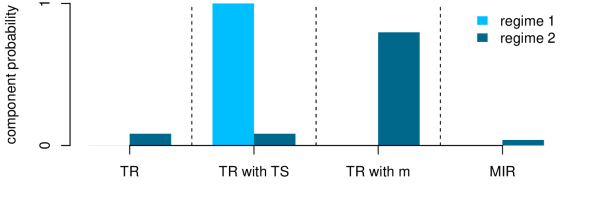
Figure 1: Posterior probabilities of the TVI components, the monetary policy reaction functions, in both regimes

Note: Figure shows the posterior probabilities of $\kappa_{n}(m)$ for four identification pattern in the monetary policy reaction function for regime one (light color) and regime two (dark color). US monetary policy shocks are identified via exclusion restrictions imposing on the contemporaneous relations either an empirical Taylor rule setting (“TR”), a TR augmented with term spread (“TR with TS”), a TR augmented with money (“TR with m”), or a money-interest rate rule (“MIR”).

Several papers argue that term spreads are a target of unconventional monetary policy as long term interest rates are the main transmission channel of the large asset purchase programs (Baumeister and Benati, 2013; Liu et al., 2019; Feldkircher and Huber, 2018; Tillmann, 2020). The monetary authority can target term spreads via the portfolio balance channel; increased asset purchases decrease the supply of long-term securities and lower long-term yields. Gagnon et al. (2011), Krishnamurthy and Vissing-Jorgensen (2011), and D’Amico and King (2013), among others, provide evidence that the large asset purchase programs during the zero lower bound period affect long-term yields. Our results extend those findings by showing that the monetary policy reaction function of the Fed accounts for the information revealed by term spreads even before the start of unconventional monetary policy since the first regime occurs mainly before 2008. This suggests that the interest rates are established with consideration to the whole bond yield curve in the spirit of Diebold et al. (2006).

In the second regime visualized by the dark color in Figure 1, the monetary authority responds simultaneously to changes in the monetary aggregate. The posterior value of the TVI component indicator for the exclusion restriction pattern based on a TR augmented by money (TR with m) is 0.8. The posterior probability of the remaining components is very low, with TR and TR with TS both having 0.08 posterior probability and the money-interest rate rule 0.04.

Our findings are in line with Belongia and Ireland (2015) supporting that after 2008 monetary policy actions lead to changes in the monetary aggregates. While the Fed officially targeted money supply before 1982, Belongia and Ireland (2015) argue that unconventional monetary policy can be seen as attempts to increase money growth. Similar to the strong support of data for money in the monetary policy rule in the second regime, the authors show that excluding a monetary measure from the interest rate rule is rejected by the data in the sample to 2007. Similarly, Lütkepohl and Woźniak (2020) find empirical evidence for monetary policy rules containing money in models identified via heteroskedasticity for data up to 2013. Neither of these papers considers rules including the term spread or time variation of the structural matrix.

The posterior means of the contemporaneous coefficients in the monetary policy reaction function, the third row of the structural matrix, with the bounds of the 90% highest density interval in parentheses,

Regime 1: $$\quad\underset{(-0.04;\ 0.23)}{0.10}y_{t}\underset{(-0.11;\ -0.04)}{-0.07}\pi_{t}\underset{(3.23;\ 3.84)}{+3.53}R_{t}\underset{(3.71;\ 4.27)}{+3.99}TS_{t}$$

Regime 2: $$\quad\underset{(-0.66;\ -0.31)}{-0.48}y_{t}\underset{(-0.09;\ 0.03)}{-0.03}\pi_{t}\underset{(8.91;\ 16.36)}{+12.60}R_{t}\underset{(-1.75;\ -0.41)}{-1.13}m_{t}$$

show notable differences across the regimes. In the first regime, interest rates and term spreads are clearly contemporaneously related. The posterior mean of the contemporaneous coefficient on term spreads in the monetary reaction function is positive, with strong evidence that it is different from zero. Interest rates react also to inflation, whereas the coefficient on output is not different from zero. In the second regime, money aggregate plays the dominant role in the policy rule for interest rates, as evidenced by a significant and relatively highest in absolute terms coefficient on this variable. This regime also observes an increase in the importance of output relative to inflation in the monetary policy reaction function. The coefficient on the latter is insignificant. This fact, together with the timing of the second regime, is in line with the shift in the emphasis in the monetary policy after 2000 described by Belongia and Ireland (2016).

3.2 Robustness of TVI

Selecting two different generalized TR identification patterns over time is remarkably robust with respect to extending or limiting the set of possible exclusion restrictions in the search. First, broadening the set of exclusion restrictions leads to the same posterior probabilities of the TVI mechanism in the monetary policy reaction function – shown in Figure 2(a) for a model which includes a fifth option setting exclusion restrictions according to a TR with stock prices.

Figure 2: Posterior probabilities of the TVI mechanism in the monetary policy reaction function for extended or restricted TVI specifications

(a) extended by TR with sp

(b) TR and TR with TS

(c) TR and TR with m

(d) TR and unrestricted

Note: Figure shows the posterior probabilities of $\kappa_{n}(m)$ for the identification pattern in the monetary policy reaction function for regime one (light color) and regime two (dark color) for three different models. Model (a) allows for TR, TR with TS, TR with m, TR with sp, and MIR. Model (b) allows for TR and TR with TS, model (c) for TR and TR with m, and model (d) for TR and unrestricted.

Second, limiting the set of possible exclusion restrictions to the TR and one generalized alternative supports the role of the term spread and money in the respective regimes. Allowing for either the TR or TR with TS as exclusion restriction patterns data support the generalized TR in the first regime with 100% posterior probability as shown in Figure 2(b). Absent the relevant alternative, the search in the second regime is uninformative placing equal probability on both specifications. Imposing exclusion restrictions either in line with the TR or TR with m, the posterior probability of the TR with m is around 80% in the second regime, exactly matching the result from our benchmark model, while it is 50% in the first regime in Figure 2(c).

When the TR is compared with an unrestricted third row of the structural matrix, the latter is strongly preferred in both regimes as shown in Figure 2(d). This shows that a rule containing the relevant alternatives such at TR with TS or TR with m is also preferred over the simple TR. Our attempts of estimating a model with an unrestricted policy rule resulted in less persistent regimes and lack of within-regime identification via heteroskedasticity. Overall, this exercise documents that whenever a policy rule preferred by the data or a rule containing it is available, the result is the same as in our benchmark model, and at the absence of it any policy rule is evenly likely.

Moreover, our analysis of an extensive set of alternative specifications changing the model setup reinforces our conclusions regarding the TVI probabilities. These alternative model specifications included those with different lag lengths from one to 12 or changes in the variables included. We used personal consumption expenditures excluding food and energy or an interpolated GDP deflator instead of CPI, interpolated GDP instead of the industrial production index, shadow rates instead of federal funds rates, monetary base as an alternative money aggregate, and added credit spreads or inflation expectations to the model. Furthermore, we changed prior set-ups by changing hyper-parameters on the priors set on the contemporaneous, autoregressive coefficients, SV or the Markov-process with no changes in the TVI probabilities.

3.3 Interpretation of the two Markov-switching regimes

Having established that data clearly support regime-specific identification of US monetary policy shock, we now take a closer look at the two estimated MS regimes.

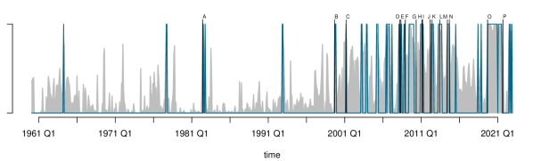
Figure 3: Regime probabilities of the Markov process

Note: Figure shows the estimated regime probabilities of the second regime (shaded areas) and the occurrences of the second regime with probability larger than 0.8 (dark color). Probabilities for the first regime are one minus the probabilities of the second regime. List of events:
A Dec 1982 peak of 1981-1982 recession B Mar 2000 dot-com bubble burst C Sep 2001 September 11 attacks D Sep 2008 bankruptcy of Lehman Brothers on September 15, 2008 E Nov 2008 FOMC announces Quantitative Easing 1 F Jun 2009 NBER declares end of the US great recession G Nov 2010 FOMC announces Quantitative Easing 2 H Aug 2011 FOMC announces to keep the federal funds rate at its effective zero lower bound “at least through mid-2013”^∗ I Sep 2011 FOMC announces Operation Twist J Sept 2012 FOMC announces Quantitative Easing 3 K Dec 2012 FOMC announces to purchase 45B$ of longer-term Treasuries per month for the future, and to keep the federal funds rate at its effective zero lower bound  L Dec 2013 FOMC announces to start lowering the purchases of longer-term Treasuries and mortgage-backed securities (to $40B and $35B per month, respectively) M Dec 2014 FOMC announces “it can be patient in beginning to normalize the stance of monetary policy” N Mar 2015 FOMC announces “an increase in the target range for the federal funds rate remains unlikely at the April FOMC meeting” O Mar 2020 start of COVID-19 pandemic. First unscheduled FOMC meeting on March 3 in response to the outbreak of the pandemic announcing to “lower the target range for the federal funds rate by 1/2 percentage point” and to “use its tools and act as appropriate to support the economy.” On March 23, FOMC statement to “continue to purchase Treasury securities and agency mortgage-backed securities in the amounts needed to support smooth market functioning”. P Mar 2022 First indications of changes in monetary policy with FOMC annoucing that one member voted against keeping the federal funds rate at the same rate. In May and June the federal funds rate was increased with the largest hikes since May 2000 and 1994, respectively.
^∗ all quotes from https://www.federalreserve.gov/newsevents/pressreleases.htm.

Figure 3 shows the estimated regime probabilities for the second regime (a gray shaded area), together with highlighted periods when the probability for the second regime is larger than 0.8 (dark-colored thick line), and specific events (black vertical lines topped by letters). Regime one is predominant in the first part of the sample until 2000. It is present in periods of rather normal economic developments (aka non-crisis times). After 2000 the second regime occurs more frequent and the periods are characterized by a mixture between the two regimes. The second regime clearly prevails during crisis periods, in particular the financial and COVID-19 ones. In the aftermaths of these events, regime 2 gains persistence. Additionally, it is present at earlier extra-ordinary times such as the peak of the 1981–1982 crisis, the burst of the dot-com bubble in March 2000, or 9/11. Beside its characterization as a crisis regime, it also predominately covers periods of unconventional monetary policy actions such as Quantitative Easing 1, Operation Twist, and several subsequent announcements of the Fed, starting in August 2011, stating that they would keep the federal funds rate at its effective zero-lower bound for a substantial period.

Table 2: Regime-specific sample moments of data and structural shocks

	data						structural shocks
	Regime 1			Regime 2			Regime 1			Regime 2
	mean	sd		mean	sd		mean	sd		mean	sd
$y_{t}$	2.72	8.40		1.46	17.36		0.00	0.97		-0.11	1.65
$\pi_{t}$	4.11	3.61		2.65	4.04		0.00	1.01		-0.04	1.13
$R_{t}$	5.67	3.66		2.54	2.74		0.03	1.05		-0.14	1.23
$TS_{t}$	0.87	1.69		1.48	1.28		-0.02	1.61		-0.07	0.76
$m_{t}$	6.45	3.84		7.41	8.53		-0.02	0.90		0.08	1.23
$sp_{t}$	7.24	51.14		6.15	54.58		0.01	0.99		-0.06	1.01

Note: Table reports sample means and standard deviations for variables and estimated structural shocks in both regimes. The regime-specific moments are given for the series in first differences for $y_{t}$, $m_{t}$, and $sp_{t}$.

As revealed by TVI, the Fed acts on the federal funds rate simultaneously with term spread movements in the first regime and money in the second. Moreover, regime-specific data and structural shocks’ sample moments reported in Table 2 attach an crisis versus non-crisis interpretation to the regimes. The regime-specific means and standard deviations of the variables display patterns characteristic to a lower level of economic activity and higher volatility. This is particularly well-evidenced for the industrial production growth rate and inflation that have considerably lower means and higher standard deviations in the second regime. The federal funds rate is on average lower and the term spread higher in the second regime while they both exhibit lower volatility then. Money is twice as volatile in the second regime. Remarkably, the differences for $sp_{t}$ are small indicating that stock market developments explain rather little in the differences across the regimes.

The sample moments characterising the structural shocks within the regimes reported in Table 2 confirm our interpretation of the second regime as the crisis one. As long as the regime-specific averages of the shocks are equal to zero in the first regime, the signs of all the shocks in the second one are negative, except for the money supply shock. The standard deviations are greater than those in the first regime, except for the term spread shock. The negative averages for industrial production, inflation, and stock price shocks indicate strong recessionary pressures from the economy in the second regime. Particularly indicative is the high in absolute terms and a negative average of the monetary policy shock reaching -14 basis points and that of the term spreads, equal to -7 basis points. This indicates that the second regime captures monetary policy that is characterized by cutting the interest rates and narrowing the bond yield curve supplemented by expanding the monetary basis. These findings confirm our labelling of the second regime as more erratic crisis periods that trigger unconventional monetary policy actions.

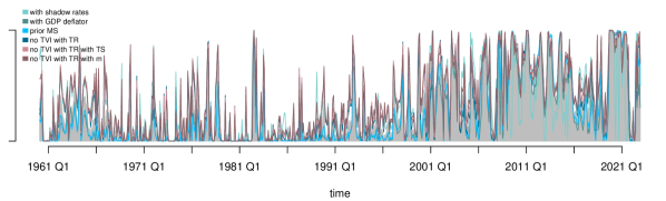
Figure 4: Regime probabilities of the Markov process across alternative model specifications

Note: Figure shows the estimated regime probabilities of the second regime for several model specifications (solid lines) together with those of the base line model (shaded area). Probabilities for the first regime are one minus the probabilities of the second regime.

We find that the regime allocations are robust to various changes in the model specification. We illustrate the role of important factors for the regime allocation by altering the measure of the monetary policy indicator and inflation, changing the prior expected duration of the Markov process, and discarding TVI. The estimated regime probabilities, shown in Figure 4, are very similar for all alternatives: for models including shadow rates of Wu and Xia (2016) as an alternative measures of short term interest rates (labeled as “with shadow rates”), using GDP deflator as measure of inflation (“with GDP deflator”), setting the expected regime duration of the Markov process to 42 months (“prior MS”), with MS but without TVI where we impose on the structural matrix restrictions according to either TR, TR with TS or TR with m (labeled by “no TVI with TR”, “no TVI with TR with TS”, “no TVI with TR with m”, respectively). Additionally, we found that models with $M=3$ states are not supported by the data as they were always characterized by occurrence at a negligible number of dates.

3.4 Within-regime identification through heteroskedasticity

Our search for regime-specific identification patterns requires that the exclusion restrictions on the monetary policy rule over-identify it and, thus, can be tested using statistical methods. We achieve this using identification via heteroskedasticity. Figure 5 plots histograms of the monetary policy shock volatility of the volatility parameter $\omega_{3}(m)$ for both regimes, $m\in\{1,2\}$. Verifying whether these parameters differ from zero implies identifying the underlying shock as argued by Lütkepohl et al. (2023). We find clear evidence for heteroskedasticity within both regimes for the monetary policy reaction function visualized by the bi-modality of the posterior distribution. The mass of the posterior distributions is away from zero, which is more pronounced in the second regime. Therefore, the monetary policy shock is identified via heteroskedasticity and our selection of identifying restrictions is valid in both regimes.

We then label the third shock as the monetary policy shock based on the exclusion restrictions imposed on the monetary policy reaction function. This is sufficient in the second regime featuring the money-augmented TR as the set of restrictions in the corresponding row of the structural matrix is unique. However, in the first regime, the exclusion restrictions selected for the third row of the structural matrix are the same as those for the fourth. Here, we additionally consider the impulse response functions to label the third structural shock as the monetary policy shock.

Figure 5: Marginal posterior and prior densities of the regime-specific volatility of the volatility parameter, $\omega_{3}$, for the monetary policy shock

Note: Figure reports histograms of the posteriors for the regime-specific monetary policy shock volatility of the volatility parameters $\omega_{3}(m)$ for regime one (light color) and regime two (dark color). The marginal prior distribution is given by the solid line. The concentration of the posterior probability mass away from zero indicates that the monetary policy shock is identified via heteroskedasticity in both regimes.

We find that the identification of the monetary policy shocks via heteroskedasticity is robust to changes of hyper-parameters in the prior distributions on contemporaneous effects, autoregressive coefficients, SV, or the Markov process. Crucially, changing the scale hyper-parameter of the prior controlling for the volatility of the volatility level by order of magnitude (we tried values ranging from 0.1 to 2) only marginally affects the posterior distribution of $\omega_{3}(m)$ in both regimes. Also, using alternative measurements for our variables, such as shadow rates instead of federal funds rates or an interpolated GDP deflator for CPI inflation, has no impact on identification via heteroskedasticity. However, there are some factors impeding identification via heteroskedasticity especially in the second regime. They include, for instance, using interpolated GDP as an economic activity measure or specifying a model with MS in the structural matrix but without TVI.

4 Effects of US monetary policy shocks with TVI

In this section we present regime-specific impulse response to a US monetary policy shock. We then focus on the role of the term spread in more detail, analyze time-variation of the effects of monetary policy shocks and a counterfactual scenario in which the monetary policy in the second regime does not emerge, and discuss the importance of TVI for solving the price puzzle.

4.1 Dynamic responses to US monetary policy shocks

We find notable differences in the dynamic responses to the US monetary policy shock across the regimes. They lead to distinguishing interpretations of the monetary policy conducted in the particular sub-periods. Based on its effects in the first regime, the monetary policy can be characterised as conventionally inflation-targeting, whereas in the second one, as strongly expansionary with specific macro-financial interactions. Our analysis is based on Figure 6 reporting the median impulse responses to a monetary policy shock decreasing interest rates by 25 basis points in the first (light color) and second (dark color) regime together with the 68% posterior highest density sets. As in the second regime the monetary policy shocks are on average negative as reported in Table 2, we discuss the effects of a negative shock.

Figure 6: Impulse response to US monetary policy shocks

(a) response of $y$

(b) response of $\pi$

(c) response of $R$

(d) response of $TS$

(e) response of $m$

(f) response of $sp$

Note: Figure shows posterior median impulse responses to a expansionary monetary policy shock of 25 basis points (solid lines) for regime 1 (light color) and regime 2 (dark color) together with 68% posterior highest density sets (shaded areas).

In the first regime, an unexpected monetary loosening leads to a persistent level shift in the federal funds rate. The response falls to the lowest point after 15 months at 77 basis points. This shock is effective in increasing inflation within the perspective of the following 19 months and with the highest impact of 0.55 pp after seven months. The effect on output is negative and statistically significant up to two years. The system features the liquidity effect with the money supply substantially and permanently increasing. In line with Ang et al. (2011), the lower interest rates decrease the slope of the bond yield curve for the following 15 months, with the trough response narrowing the term spread by 118 basis points after one month. They also lead to a sharp increase in stock prices.

Moreover, in line with the inflation-targeting goal, our results imply that an unexpected monetary tightening is effective in curbing inflation in the first regime. An increase in the federal funds rate induced by a positive monetary policy shock would result in a statistically significant decrease in inflation reaching up to 0.55 pp after seven months.

In the second regime, a negative monetary policy shock decreases the federal funds rate permanently but slightly more moderately than in the first regime. In this regime, the monetary policy is strongly expansionary as output increases permanently and by nearly 1% within the first year. At the same time, inflation’s response is negligible and only significant at the horizon of four months following the shock reaching 0.2 pp. These phenomena are in line with the Fed’s shifting emphasis from inflation to output after 2000, discussed in Section 3.1.

In these times of crises, the liquidity effect is positive and even more pronounced in this regime with the response stronger by 1 pp nearly at all horizons. The slope of the bond yield curve is only slightly affected as the term spread widens by 30 basis points after one month, strengthening the conclusion by Tillmann (2020) on time variation in this effect. The response cools off gradually but remains significant at all horizons. The stock prices contract by nearly 2% on impact – the reaction gradually fading out within ten months. This result closely follows the change over time of the impulse responses reported by Galí and Gambetti (2015) that the authors explained by the existence of rational bubbles in the stock market.

These effects are in line with the characterisation of the monetary policy in the US as unconventional in the periods aligning with the second regime. The main objectives of these policies were to stimulate the economy in the aftermaths of the crises and provide liquidity, all of which was implemented without substantially increasing inflation in line with “missing inflation“ during the 2010s (see Bobeica and Jarocinski, 2019), a period which is covered by the second regime.

Our results indicate time-variation in the monetary policy shock identification. Time-varying parameters and identification play a crucial role in the interpretability of the shocks. It is not obtained if any of these features are omitted from the model formulation. Nevertheless, our results are robust to many other alterations in the specification. The impulse responses keep their shapes irrespectively of changing the lag order as long as it is greater than 4, replacing the variables by alternative measurements, such as using interpolated real GDP or shadow rates for industrial production or interest rates, respectively, or altering the prior hyper-parameter values. Finally, TVI allows us to obtain distinctive interpretations of the monetary policy effects in both MS regimes. We show other aspects of the monetary policy in the second regime, characterising it as unconventional by analysing the effects of the term spread shock.

4.2 Dynamic responses to US term spread shocks

To understand the differences of the term spread response to the monetary policy shock across regimes, we relate it to the responses of interest rates, term spread, and money to a term spread shock, shown in Figure 7. The spread shock – an unexpected narrowing of the term spread – describes an unanticipated change in the financial markets such as shifts in liquidity or risk preferences, or inflation expectations. When the federal funds rate is at its effective zero lower bound, a term spread shock can be interpreted as a result of the Feds bond purchase programs (Baumeister and Benati, 2013). Capturing different monetary policy facets with multiple shocks is also applied by the large literature following Gürkaynak et al. (2005).

Figure 7: Impulse response to US term spread shocks

(a) response of $R$

(b) response of $TS$

(c) response of $m$

Note: Figure shows posterior median impulse responses to a negative spread shock of 10 basis points (solid lines) for regime (light color) and regime 2 (dark color) together with 68% posterior credibility sets (shaded areas).

A negative spread shock of 10 basis points lowers terms spreads for at least two years in both regimes. The reaction in the first regime is stronger and lasts longer. We find notable differences across regimes for the response of the federal funds rate and money.

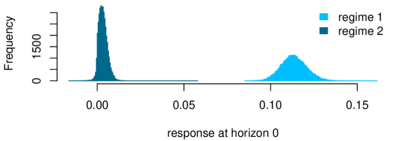
Figure 8: Zero horizon response of interest rates to US term spread shocks

Note: Figure shows posterior distribution of zero horizon response of interest rates to a negative spread shock of 10 basis points for regime (light color) and regime 2 (dark color). For regime 2 only those draws are taken where TR with m was selected.

The short term interest rates increase in the first regime by 0.11 pp on impact and peaks at 0.19 pp within one year. In the second regime, interest rates do not move within one month and decrease afterwards by $-$0.04 pp at maximum. The differences in the impact response are remarkable, visualized in the histograms of the zero horizon responses in Figure 8. The posterior estimates are positive and clearly away from zero in the first regime, while in the second the posterior distribution of the estimated impact response is tightly centered around zero with considerable mass at zero. In the second regime, which predominately covers the period of the zero-lower-bound environment, monetary policy interventions can have a narrowing effect on the term spread while the short term interest rate does not move. That finding provides empirical evidence for the restriction that short term interest rates do not react to a term spread shock for four quarters imposed by Baumeister and Benati (2013) and Feldkircher and Huber (2018). However, we found support for the restriction the other authors assume only for the second regime, and we obtained it in the process of estimation using TVI rather than imposing it in a system otherwise identified by sign restrictions. Nevertheless, this result confirms the identification of a pure term spread shock flattening the bond yield curve without affecting the interest rate contemporaneously that characterises unconventional monetary policy according to Baumeister and Benati (2013).

Money increases in reaction to a negative spread shock in the second regime and decreases in the first. The effect is long lasting in both regimes. The positive reaction of money in the second regime – which is predominate during unconventional monetary policy periods – aligns with the interpretation of the term spread shock as mirroring quantitative easing (see Baumeister and Benati, 2013; Feldkircher and Huber, 2018; Liu et al., 2019).

4.3 What does monetary policy do?

How effective was the Fed in reaching its dual mandate of price stability and economic growth over time? To quantify this, we show the cumulative effects of monetary policy shocks over one year at each point in time for industrial production and inflation in Figure 9.

Figure 9: Cumulative effects of the last year’s monetary policy shocks over time

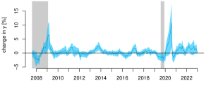
(a) $y$

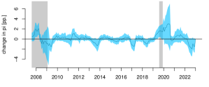
(b) $\pi$

Note: Figure shows the impulse responses of industrial production and inflation to monetary policy shocks cumulated over one year (solid lines) together with the 68% highest posterior density set, starting in January 2008. The gray shaded areas mark the NBER recessions during the reported period.

Post GFC and COVID-19 crisis monetary policy had buffering effects. After the crisis, expansionary monetary policy lead to sharp increases in economic activity reaching 6.5% in August 2009 and 10.8% in January 2021. The effects are clearly different from zero then. Compared to these episodes, monetary policy shocks lead to minor changes in industrial production in the remaining periods.

The cumulative responses of inflation to monetary policy shocks are positive and clearly different from zero in the aftermaths of the GFC and COVID-19 crisis. Mitigating the recessions comes at the cost of higher inflation in the short term. For a year, starting in mid-2009, monetary policy had a disinflationary effect, reaching up to -1.5 pp in November 2009. The effect seems not statistically different from zero, though. During the period starting in 2010 up to early 2020 inflation reacted little to recent monetary policy shocks. The sharp inflationary effect in late 2020 reached 3 pp. Finally, tightening of the monetary policy after 2022 was deflationary with the strongest cumulative response at the level of -2 pp in February 2023.

Overall, our model indicates that in the last fifteen years, US monetary policy targeted mainly sharp economic crises providing a cushioning effect on the economy. Their actions were strongly expansionary in the aftermaths of the global financial and COVID-19 crises. The stimuli came with a delay and put substantial inflationary pressure. In normal times, the central bank intervenes to a minor extent.

4.4 What if monetary policy as conducted in the second regime never emerged?

The interventions of the Fed were particularly essential after the GFC and COVID-19 crisis. Since systematic monetary policy predominately can be characterized by a TR augmented with money during these periods, we further investigate the time-varying effects of these policy actions. Specifically, we ask the question of how economic activity, inflation, short-term interest rates, term spread, money, and stock prices would have evolved if the monetary policy as conducted in the second regime never emerged.

To that end, we generate a counterfactual scenario in which the economic developments propagate according to the monetary policy rule from the first regime and compare it to the actual values predicted by our unaltered model. Consequently, we first isolate standardized shocks deprived of the mean, volatility, and contemporaneous relationships and propagate them according to the parameter values where the third row of the structural matrix – the monetary policy reaction function – and the corresponding volatility of the volatility parameter include the values from the first regime only. Subsequently, we calculate counterfactual values of the economic outcomes.

Figure 10: Counterfactual and actual values of the time series

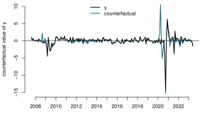
(a) $y$

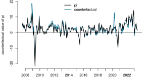
(b) $\pi$

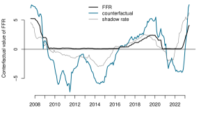
(c) $R$

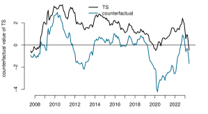
(d) $TS$

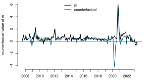
(e) $m$

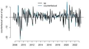
(f) $sp$

Note: Figure shows the actual values of the six time series (dark lines) together with the counterfactual value (light lines) starting in January 2008. The analysis transforms $y_{t}$, $m_{t}$, and $sp_{t}$ to their growth rates.

Figure 10 shows the counterfactual values in comparison to the the actual values of the time series for January 2008 until June 2023. If monetary policy as conducted in the second regime did not occur, inflation would be on average 1 pp higher after the GFC as reported in Figure 10(b). This result is in line with the stronger impulse response of inflation in the first regime combined with on average negative monetary policy shocks for the considered period. We also link this result to the missing inflation interpretation by Bobeica and Jarocinski (2019). In our model, if the second regime in the monetary policy reaction function did not emerge and inflation was forecasted using the parameter values and identification from the first regime, the model would predict a much higher inflation rate after 2008 than that which eventuated.

Short term interest rates would be on average 1.4 pp lower. During zero lower bound periods including the COVID-19 pandemic, the counterfactual value of the federal funds rates is negative. Indeed, albeit more volatile, it follows closely the movements in the shadow rate represented by the gray line in Figure 10(c). The term spread would be considerably lower, especially from 2011 to 2016, on average by around 1.2 pp. A similar result is reported by Baumeister and Benati (2013) and, as the authors argue, it does not contradict the stabilizing effects of the monetary policy during this period. This is supported by the lower standard deviations of the term spread shock in regime 2 reported in Table 2.

Money and industrial production growth rates as well as stock returns are not substantially different from the actual values except for specific episodes. For instance, in the second quarter of 2020, the counterfactual value of money growth is much lower and those of stock returns and industrial production growth are higher than the actual values. Money growth is also visibly lower in the counterfactual scenario throughout 2021. Summarizing, our counterfactual analysis provides evidence that monetary policy as conducted in the second regime was effective in lowering inflation, providing liquidity in the time of stress, and stabilizing the bond yield curve after 2008.

4.5 Solving the price puzzle

Our results show that unexpected contractionary monetary policy actions effectively lower or keep the same level of inflation. Thus, our findings do not exhibit a price puzzle as frequently discussed in the literature for SVARs. We find two crucial conditions under which our results do not feature the price puzzle. First, we include as measure of inflation the price index in log first differences. Including prices in their level leads to increasing prices in response to a contractionary monetary policy shock. Note, that the inflation series includes a unit root as other series do while the log CPI price index is integrated of order two. Second, TVI is essential to avoid model misspecification resulting in the puzzle. To illustrate the latter conclusion, we estimate models with MS but without TVI. We investigate three different models where we impose restrictions on the structural matrix according to either TR, TR with TS or TR with m.

Figure 11: Inflation response to US monetary policy shocks for models without TVI

(a) no TVI with TR

(b) no TVI with TR with TS

(c) no TVI with TR with m

Note: Figure shows posterior median impulse responses of inflation to an expansionary monetary policy shock of 25 basis points (solid lines) for regime (light color) and regime 2 (dark color) together with 68% posterior credibility sets (shaded areas) for three different models (in subplots). The models are without TVI and the imposed restrictions to identify a monetary policy shock are according to either TR, TR with TS or TR with m

In Figure 11, reporting inflation impulse responses for these three models, inflation decreases in response to an expansionary monetary policy shock in both regimes and, thus, exhibiting the price puzzle. Hence, TVI allows for an enriched analysis of the time-varying nature of monetary policy effects and enhances the interpretability of impulse responses. We attribute this finding to a correct policy rule specification that TVI facilitates. An additional aspect of the miss-specification in regime 2 in Figure 11(b) and regime 1 in Figure 11(c) is that the identification fails, generating unnecessarily wide credibility sets.

5 Conclusions

We propose a new Bayesian structural vector autoregression which allows for time-varying identification. Our model facilitates a data-driven search of regime-specific exclusion restriction patterns. It features persistent Markov-switching regimes in the structural matrix and the volatility of the volatility as well as structural shock variances evolving at a much higher frequency following stochastic volatility. These components allow us to study time-variation in monetary policy identification, time-varying impulse responses, and provide an easy way to check identification via heteroskedasticity within each regime as a validity condition of regime-specific identification.

We find solid and robust support for time-variation in US monetary policy shock identification. Time-varying identification is essential to characterise unconventional monetary policy in the aftermath of the global financial and COVID-19 crises. Moreover, correctly specifying the model in the state-dependent setting enables sharp identification in each of the Markov-switching regimes, and provides wide interpretability of various reported outcomes.

Our results show that in the last fifteen years, monetary policy was conducted unconventionally and acted mainly as a buffer against the adverse economic effects of the financial crisis and the COVID-19 pandemic. The Fed provided stimuli to economic activity and liquidity to the market. At the same time, the central bank effectively curbs inflation which in the absence of extraordinary means, would be on average one pp higher.

Appendix A Data

$ip$	log industrial production (INDPRO), Total Index, Index 2017=100, Seasonally Adjusted, Source: Board of Governors of the Federal Reserve System (2023b), retrieved from FRED database [accessed 15.08.2023]
$cpi$	log difference of consumer price index (CPALTT01USM661S), Total All Items, Index 2015=100, Seasonally Adjusted, Source: Organization for Economic Co-operation and Development (2023), retrieved from FRED database [accessed 15.08.2023]
$R$	federal funds rate (DFF), Source: Board of Governors of the Federal Reserve System (2023a), retrieved from FRED database [accessed 15.08.2023]
$TS$	$ts=r_{L}-r$, 10-year Treasury constant maturity rate minus federal funds rate (T10YFFM), Source: Federal Reserve Bank of St. Louis (2023)
$m$	log M2 (M2SL), Billions of Dollars, Seasonally Adjusted, Source: Board of Governors of the Federal Reserve System (2023c), retrieved from FRED database [accessed 15.08.2023]
$sp$	log S&P500 stock price index, monthly average of closing price (^GSPC), Source: yahoo finance (2023) [accessed 15.08.2023]
shadow rates	United States shadow fed funds rate of Wu and Xia (2016), downloaded at https://sites.google.com/view/jingcynthiawu/shadow-rates [accessed 15.08.2023]
GDP deflator	interpolated, log difference of Gross Domestic Product: Implicit Price Deflator (GDPDEF); Index Apr 1947=100, Seasonally Adjusted, Source: U.S. Bureau of Economic Analysis (2023), retrieved from FRED database [accessed 15.08.2023]

Appendix B Gibbs sampler

For simplicity, we write the VAR model in compact form

$$\mathbf{y}_{t} =\mathbf{A}\mathbf{x}_{t}+\boldsymbol{\varepsilon}_{t}$$ (17)

where the $N\times(Np+d)$-matrix $\mathbf{A}=\begin{bmatrix}\mathbf{A}_{1}&\dots&\mathbf{A}_{p}&\mathbf{A}_{d}\end{bmatrix}$ collects autoregressive and constant parameters and the $(Np+d)$-vector $\mathbf{x}_{t}=\begin{bmatrix}\mathbf{y}_{t-1}^{\prime}&\dots&\mathbf{y}_{t-p}^{\prime}&\mathbf{d}_{t}^{\prime}\end{bmatrix}^{\prime}$ contains lagged endogenous variables and constant terms.

Sampling parameters in the structural matrix

To estimate the parameters in the structural matrix, we use a Gibbs sampler. The full conditional posterior distribution of the unrestricted elements in regime $m$, equation $n$, and TVI component $k$ is generalised-normal, proportional to

$$|\det\left(\mathbf{B}_{m.\mathbf{k}}\right)|^{T_{m}}\exp\left\{-\frac{1}{2}\mathbf{b}_{n.m.k}\mathbf{V}_{n.m.k}\overline{\boldsymbol{\Omega}}_{B.nm}^{-1}\mathbf{V}_{n.m.k}^{\prime}\mathbf{b}_{n.m.k}^{\prime}\right\}$$ (18)

where $\mathbf{B}_{m.\mathbf{k}}$ is the matrix from regime $m$ and TVI component $k$, with scale matrix

$$\overline{\boldsymbol{\Omega}}_{B.nm}^{-1} =\gamma_{B.n}^{-1}\mathbf{I}_{N}+\sum_{t:s_{t}=m}(\mathbf{y}_{t}-\mathbf{A}\mathbf{x}_{t})(\mathbf{y}_{t}-\mathbf{A}\mathbf{x}_{t})^{\prime}$$ (19)

where $T_{m}$ is the number of observations in regime $m$. Within each regime, we sample the structural matrix and the TVI indicators jointly.

1. Sample parameters of the structural matrix: $\mathbf{B}$ row-by-row following the algorithm by Waggoner and Zha (2003) by sampling $K$ vectors $\mathbf{b}_{n.m.k}$ from (18) given $\kappa(m)=k$ for all $k\in\{1,\dots,K\}$.

2. Sample TVI indicators: by computing the conditional posterior probabilities of each of these TVI components, $\overline{p}_{n.m.k}$, proportional to the product of the likelihood function, $L(\theta\mid\mathbf{Y}_{T})$, and the prior distributions:

   $$\overline{p}_{n.m.k} \propto L(\theta\mid\mathbf{Y}_{T},\kappa(m)=k)p\left(\mathbf{B}_{n.m.k}\mid\gamma_{B},\kappa(m)=k\right)p\left(\kappa(m)=k\right).$$ (20)

   Sample the TVI indicator from the multinomial distribution using the probabilities $\overline{p}_{n.m.k}$ for $k=1,\dots,K$, and return the draw from the joint posterior $\left(\mathbf{b}_{n.m.k},k\right)$.

3. Sample structural hyper-parameters: $\gamma_{B.n}$, $\underline{s}_{B.n}$, and $\underline{s}_{\gamma_{B}}$ from their respective full conditional posterior distributions:

   $$\gamma_{B.n}\mid\mathbf{B}_{n.m.k},k,\underline{s}_{B.n} \sim\mathcal{IG}2\left(\underline{s}_{B.n}+\sum_{m}\mathbf{b}_{n.m.k_{n}}\mathbf{b}_{n.m.k_{n}}^{\prime},\quad\underline{\nu}_{B}+\sum_{m}r_{n.m.k_{n}}\right)$$ (21)

   $$\underline{s}_{B.n}\mid\gamma_{B},\underline{s}_{\gamma_{B}} \sim\mathcal{G}\left((\underline{s}_{\gamma_{B}}^{-1}+(2\gamma_{B.n})^{-1})^{-1},\underline{\nu}_{\gamma_{B}}+0.5\underline{\nu}_{B}\right)$$ (22)

   $$\underline{s}_{\gamma_{B}}\mid\underline{s}_{B} \sim\mathcal{IG}2\left(\underline{s}_{s_{B}}+2\sum_{n=1}^{N}\underline{s}_{B.n},\underline{\nu}_{s_{B}}+2N\underline{\nu}_{\gamma_{B}}\right)$$ (23)

If TVI is not implemented in a particular row, sample $\mathbf{b}_{n.m}$ bypassing Step 2 of the algorithm.

Sampling of the remaining parameters

Estimation of the remaining is implemented by the Gibbs sampler. Our emphasis was put on the selection of the most efficient sampling techniques that would facilitate estimation in larger systems of variables for which the dimension of the parameter space grows rapidly.

The rows of the transition probabilities matrix, $\mathbf{P}$, and the initial state probabilities vector, $\boldsymbol{\pi}_{0}$, are all sampled from independent $M$-variate Dirichlet full conditional posterior distributions as in Frühwirth-Schnatter (2006). The sampling procedure for the Markov process realisations follows the forward-filtering backward-sampling algorithm proposed by Chib (1996).

Sampling autoregressive parameters

We follow Chan et al. (2022) and sample the autoregressive parameters of the $\mathbf{A}$ matrix efficiently row-by-row, where the $n\textsuperscript{th}$ row is denoted by $[\mathbf{A}]_{n\cdot}$. Denote by $\mathbf{A}_{n=0}$ the $\mathbf{A}$ matrix with its $n\textsuperscript{th}$ row set to zeros. To derive the sampler for the row of the autoregressive matrix, rewrite the structural form equation (2) in an equivalent form as:

$$\mathbf{B}_{m.k}\left(\mathbf{y}_{t}-\mathbf{A}_{n=0}\mathbf{x}_{t}\right) =\left([\mathbf{B}_{m.k}]_{\cdot n}\otimes\mathbf{x}_{t}^{\prime}\right)[\mathbf{A}]^{\prime}_{n\cdot}+\boldsymbol{\varepsilon}_{t}$$ (24)

Define an $n\times 1$ vector $\mathbf{z}_{t}^{n}=\mathbf{B}_{m.k}\left(\mathbf{y}_{t}-\mathbf{A}_{n=0}\mathbf{x}_{t}\right)$ and an $N\times(Np+d)$ matrix $\mathbf{Z}_{t}^{n}=\left([\mathbf{B}_{m.k}]_{\cdot n}\otimes\mathbf{x}_{t}^{\prime}\right)$ and rewrite equation (24) as:

$$\mathbf{z}_{t}^{n} =\mathbf{Z}_{t}^{n}[\mathbf{A}]^{\prime}_{n\cdot}+\boldsymbol{\varepsilon}_{t},$$ (25)

where the shocks follow the normal distribution defined in equation (4). This results in the multivariate normal full conditional posterior distribution for the rows of $\mathbf{A}$:

$$[\mathbf{A}]^{\prime}_{n\cdot}\mid\mathbf{Y}_{T},[\mathbf{A}]_{n=0},\mathbf{B}_{m.k},\boldsymbol{\sigma}^{2}_{1},\dots\boldsymbol{\sigma}^{2}_{T},\gamma_{A.n} \sim\mathcal{N}_{Np+d}\left(\overline{\boldsymbol{\Omega}}_{A.n}\overline{\mathbf{m}}_{A.n}^{\prime},\overline{\boldsymbol{\Omega}}_{A.n}\right)$$ (26)

$$\overline{\boldsymbol{\Omega}}_{A.n}^{-1} =\gamma_{A.n}^{-1}\underline{\boldsymbol{\Omega}}_{A}^{-1}+\sum_{t}\mathbf{Z}_{t}^{n\prime}\operatorname{diag}\left(\boldsymbol{\sigma}_{t}^{2}\right)^{-1}\mathbf{Z}_{t}^{n}$$ (27)

$$\overline{\mathbf{m}}_{A.n}^{\prime} =\gamma_{A.n}^{-1}\underline{\boldsymbol{\Omega}}_{A}^{-1}\underline{\mathbf{m}}_{A.n}^{\prime}+\sum_{t}\mathbf{Z}_{t}^{n\prime}\operatorname{diag}\left(\boldsymbol{\sigma}_{t}^{2}\right)^{-1}\mathbf{z}_{t}^{n}$$ (28)

Finally, the hyper-parameters of the autoregressive shrinkage hierarchical prior are sampled from their respective full conditional posterior distributions:

$$\gamma_{A.n}\mid[\mathbf{A}]_{n\cdot},\underline{s}_{A.n} \sim\mathcal{IG}2\left(\underline{s}_{A.n}+\left([\mathbf{A}]_{n\cdot}-\underline{\mathbf{m}}_{A.n}\right)\underline{\boldsymbol{\Omega}}_{A.n}^{-1}\left([\mathbf{A}]_{n\cdot}-\underline{\mathbf{m}}_{A.n}\right)^{\prime},\quad\underline{\nu}_{A}+Np+d\right)$$ (29)

$$\underline{s}_{A.n}\mid\gamma_{A.n},\underline{s}_{\gamma_{A}} \sim\mathcal{G}\left((\underline{s}_{\gamma_{A}}^{-1}+(2\gamma_{A.n})^{-1})^{-1},\underline{\nu}_{\gamma_{A}}+0.5\underline{\nu}_{A}\right)$$ (30)

$$\underline{s}_{\gamma_{A}}\mid\underline{s}_{A} \sim\mathcal{IG}2\left(\underline{s}_{s_{A}}+2\sum_{n=1}^{N}\underline{s}_{A.n},\underline{\nu}_{s_{A}}+2N\underline{\nu}_{\gamma_{A}}\right)$$ (31)

Sampling stochastic volatility parameters

Gibbs sampler is facilitated using the auxiliary mixture sampler proposed by Omori et al. (2007).

Specify the $n\textsuperscript{th}$ structural shock as:

$$u_{n.t}=\exp\left\{\frac{1}{2}\omega_{n}(s_{t})h_{n.t}\right\}z_{n.t},$$ (32)

where $z_{n.t}$ is a standard normal innovation. Transform this equation by squaring and taking the logarithm of both sides obtaining:

$$\widetilde{u}_{n.t}=\omega_{n}(s_{t})h_{n.t}+\widetilde{z}_{n.t},$$ (33)

where $\widetilde{u}_{n.t}=\log u_{n.t}^{2}$ and $\widetilde{z}_{n.t}=\log z_{n.t}^{2}$. The distribution of $\widetilde{z}_{n.t}$ is $\log\chi^{2}_{1}$. This non-standard distribution is approximated precisely by a mixture of ten normal distributions defined by Omori et al. (2007). This mixture of normals is specified by $q_{n.t}=1,\dots,10$ – the mixture component indicator for the $n\textsuperscript{th}$ equation at time $t$, the normal component probability $\pi_{q_{n.t}}$, mean $\mu_{q_{n.t}}$, and variance $\sigma^{2}_{q_{n.t}}$. The latter three parameters are fixed and given in Omori et al. (2007), while $q_{n.t}$ augments the parameter space and is estimated. Its prior distribution is multinomial with probabilities $\pi_{q_{n.t}}$.

Define $T\times 1$ vectors: $\mathbf{h}_{n}=\begin{bmatrix}h_{n.1}&\dots&h_{n.T}\end{bmatrix}^{\prime}$ collecting the log-volatilities, $\mathbf{q}_{n}=\begin{bmatrix}q_{n.1}&\dots&q_{n.T}\end{bmatrix}^{\prime}$ collecting the realizations of $q_{n.t}$ for all $t$, $\boldsymbol{\mu}_{\mathbf{q}_{n}}=\begin{bmatrix}\mu_{q_{n.1}}&\dots&\mu_{q_{n.T}}\end{bmatrix}^{\prime}$, and $\boldsymbol{\sigma}^{2}_{\mathbf{q}_{n}}=\begin{bmatrix}\sigma^{2}_{q_{n.1}}&\dots&\sigma^{2}_{q_{n.T}}\end{bmatrix}^{\prime}$ collecting the $n\textsuperscript{th}$ equation auxiliary mixture means and variances, $\widetilde{\mathbf{U}}_{n}=\begin{bmatrix}\widetilde{u}_{n.1}&\dots&\widetilde{u}_{n.T}\end{bmatrix}^{\prime}$, and $\boldsymbol{\omega}_{n}=\begin{bmatrix}\omega_{n}(s_{1})&\dots&\omega_{n}(s_{T})\end{bmatrix}^{\prime}$ collecting the volatility of the volatility parameters according to their current time assignment based on the sampled realizations of the Markov process. Whenever a subscript on these vectors is extended by the Markov process’ regime indicator $m$ it means that the vector contains only the $T_{m}$ observations for $t$ such that $s_{t}=m$, e.g., $\widetilde{\mathbf{U}}_{n.m}$. Finally, define a $T\times T$ matrix $\mathbf{H}_{\rho_{n}}$ with ones on the main diagonal, value $-\rho_{n}$ on the first subdiagonal, and zeros elsewhere, and a $T_{m}\times T_{m}$ matrix $\mathbf{H}_{\rho_{n}.m}$ with rows and columns selected according to the Markov state allocations such that $s_{t}=m$. Sampling latent volatilities $\mathbf{h}_{n}$ proceeds independently for each $n$ from the following $T$-variate normal distribution parameterized following Chan and Jeliazkov (2009) in terms of its precision matrix $\overline{\mathbf{V}}^{-1}_{\mathbf{h}_{n}}$ and location vector $\overline{\mathbf{h}}_{n}$ as:

$$\mathbf{h}_{n}\mid\mathbf{Y}_{T},\mathbf{s}_{n},\mathbf{q}_{n},\mathbf{B},\mathbf{A},\boldsymbol{\omega}_{n},\rho_{n} \sim\mathcal{N}_{T}\left(\overline{\mathbf{V}}_{\mathbf{h}_{n}}\overline{\mathbf{h}}_{n},{}\overline{\mathbf{V}}_{\mathbf{h}_{n}}\right)$$ (34)

$$\overline{\mathbf{V}}_{\mathbf{h}_{n}}^{-1} =\operatorname{diag}\left(\boldsymbol{\omega}_{n}^{2}\right)\operatorname{diag}\left(\boldsymbol{\sigma}^{-2}_{\mathbf{q}_{n}}\right)+\mathbf{H}_{\rho_{n}}^{\prime}\mathbf{H}_{\rho_{n}}$$ (35)

$$\overline{\mathbf{h}}_{n} =\operatorname{diag}\left(\boldsymbol{\omega}_{n}\right)\operatorname{diag}\left(\boldsymbol{\sigma}^{-2}_{\mathbf{q}_{n}}\right)\left(\widetilde{\mathbf{u}}_{n}-\boldsymbol{\mu}_{\mathbf{q}_{n}}\right)$$ (36)

The precision matrix, $\overline{\mathbf{V}}_{\mathbf{h}_{n}}^{-1}$, is tridiagonal, which greatly leads to a simulation smoother proposed by McCausland et al. (2011).

The regime-dependent volatility of the volatility parameters are sampled independently from the following normal distribution:

$$\omega_{n}(m)\mid\mathbf{Y}_{m},\mathbf{s}_{n.m},\mathbf{s}_{n.m},\mathbf{h}_{n.m},\sigma_{\omega_{n}}^{2} \sim\mathcal{N}\left(\overline{v}_{\omega_{n.m}}\overline{\omega}_{n.m},{}\overline{v}_{\omega_{n.m}}\right)$$ (37)

$$\overline{v}_{\omega_{n.m}}^{-1} =\mathbf{h}_{n.m}^{\prime}\operatorname{diag}\left(\boldsymbol{\sigma}_{\mathbf{q}_{n}.m}^{-2}\right)\mathbf{h}_{n.m}+\sigma_{\omega_{n}}^{-2}$$ (38)

$$\overline{\omega}_{n} =\mathbf{h}_{n.m}^{\prime}\operatorname{diag}\left(\boldsymbol{\sigma}_{\mathbf{q}_{n}.m}^{-2}\right)\left(\widetilde{\mathbf{u}}_{n.m}-\boldsymbol{\mu}_{\mathbf{q}_{n}.m}\right)$$ (39)

The autoregressive parameters of the SV equations are sampled independently from the truncated normal distribution using the algorithm proposed by Robert (1995):

$$\rho_{n}\mid\mathbf{Y}_{T},\mathbf{h}_{n}\sim\mathcal{N}\left(\left(\sum_{t=0}^{T-1}h_{n.t}^{2}\right)^{-1}\left(\sum_{t=1}^{T}h_{n.t}h_{n.t-1}\right),{}\left(\sum_{t=0}^{T-1}h_{n.t}^{2}\right)^{-1}\right)\mathcal{I}\left(|\rho_{n}|<1\right).$$ (40)

The prior variances of parameters $\omega_{n}(m)$, $\sigma_{\omega_{n}}^{2}$, are a posteriori independent and sampled from the following generalized inverse Gaussian full conditional posterior distribution:

$$\sigma_{\omega_{n}}^{2}\mid\mathbf{Y}_{T},\omega_{n}(1),\dots,\omega_{n}(M) \sim\mathcal{GIG}\left(M\underline{A}-\frac{1}{2},{}\sum_{m}\omega^{2}_{n}(m),{}\frac{2}{\underline{S}}\right)$$ (41)

The auxiliary mixture indicators $q_{n.t}$ are each sampled independently from a multinomial distribution with the probabilities proportional to the product of the prior probabilities $\pi_{q_{n.t}}$ and the conditional likelihood function.

Finally, proceed to the ancillarity-sufficiency interweaving sampler proposed by Kastner and Frühwirth-Schnatter (2014). Our implementation proceeds as follows: Having sampled random vector $\mathbf{\mathbf{h}}_{n}$ and parameters $\omega_{n}(m)$, compute the parameters of the centered parameterization $\tilde{h}_{n.t}=\omega_{n}(m)h_{n.t}$ and $\sigma_{\upsilon_{n}}^{2}=\omega^{2}_{n}(m)$. Then, sample $\sigma_{\upsilon_{n}.m}^{2}$ from the generalised inverse Gaussian full conditional posterior distribution:

$$\sigma_{\upsilon_{n}.m}^{2}\mid\mathbf{Y}_{m},\tilde{\mathbf{h}}_{n.m},\sigma_{\omega_{n}}^{2}\sim\mathcal{GIG}\left(-\frac{T_{m}-1}{2},{}\tilde{\mathbf{h}}_{n.m}^{\prime}\mathbf{H}_{\rho_{n}.m}^{\prime}\mathbf{H}_{\rho_{n}.m}\tilde{\mathbf{h}}_{n.m},{}\sigma_{\omega_{n}}^{-2}\right)$$ (42)

using the algorithm introduced by Hörmann and Leydold (2014). Resample $\rho_{n}$ using the full conditional posterior distribution from equation (40) where the vector $\mathbf{h}_{n}$ is replaced by $\tilde{\mathbf{h}}_{n}$. Finally, compute $\omega_{n}(m)=\pm\sqrt{\sigma_{\upsilon_{n}.m}^{2}}$ and $h_{n.t}=\frac{1}{\omega_{n}(m)}\tilde{h}_{n.t}$ and return them as the MCMC draws for these parameters.

References

- Andrés et al. (2006) Andrés, J., López-Salido, J.D., Vallés, J., 2006. Money in an Estimated Business Cycle Model of the Euro Area. Economic Journal 116, 457–477.
- Ang et al. (2011) Ang, A., Boivin, J., Dong, S., Loo-Kung, R., 2011. Monetary Policy Shifts and the Term Structure. The Review of Economic Studies 78, 429–457.
- Arias et al. (2018) Arias, J.E., Rubio-Ramírez, J.F., Waggoner, D.F., 2018. Inference based on structural vector autoregressions identified with sign and zero restrictions: Theory and applications. Econometrica 86, 685–720.
- Bacchiocchi et al. (2017) Bacchiocchi, E., Castelnuovo, E., Fanelli, L., 2017. Gimme a Break: Identification and Estimation of the Macroeconomic Effects of Monetary Policy Shocks in the US. Macroeconomic Dynamics 22, 1613–1651.
- Bacchiocchi and Fanelli (2015) Bacchiocchi, E., Fanelli, L., 2015. Identification in Structural Vector Autoregressive Models with Structural Changes, with an Application to US Monetary Policy. Oxford Bulletin of Economics and Statistics 77, 761–779.
- Baumeister and Benati (2013) Baumeister, C., Benati, L., 2013. Unconventional Monetary Policy and the Great Recession: Estimating the Macroeconomic Effects of a Spread Compression at the Zero Lower Bound. International Journal of Central Banking 9, 165–212.
- Belongia and Ireland (2015) Belongia, M.T., Ireland, P.N., 2015. Interest Rates and Money in the Measurement of Monetary Policy. Journal of Business & Economic Statistics 33, 255–269.
- Belongia and Ireland (2016) Belongia, M.T., Ireland, P.N., 2016. The evolution of U.S. monetary policy: 2000–2007. Journal of Economic Dynamics and Control 73, 78–93.
- Board of Governors of the Federal Reserve System (2023a) Board of Governors of the Federal Reserve System, 2023a. Federal Funds Effective Rate [DFF]. Data. URL: https://fred.stlouisfed.org/series/DFF. Retrieved from FRED database [accessed August 15, 2023].
- Board of Governors of the Federal Reserve System (2023b) Board of Governors of the Federal Reserve System, 2023b. Industrial Production: Total Index [INDPRO]. Data. URL: https://fred.stlouisfed.org/series/INDPRO. Retrieved from FRED database [accessed August 15, 2023].
- Board of Governors of the Federal Reserve System (2023c) Board of Governors of the Federal Reserve System, 2023c. M2 [M2SL]. Data. URL: https://fred.stlouisfed.org/series/M2SL. Retrieved from FRED database [accessed August 15, 2023].
- Bobeica and Jarocinski (2019) Bobeica, E., Jarocinski, M., 2019. Missing Disinflation and Missing Inflation: A VAR Perspective. International Journal of Central Banking 15, 199–232.
- Boivin et al. (2010) Boivin, J., Kiley, M.T., Mishkin, F.S., 2010. Chapter 8 - how has the monetary transmission mechanism evolved over time?, Elsevier. volume 3 of Handbook of Monetary Economics, pp. 369 – 422.
- Camehl and von Schweinitz (2023) Camehl, A., von Schweinitz, G., 2023. What explains international interest rate co-movement? IWH Discussion Papers 3/2023. Halle Institute for Economic Research (IWH).
- Castelnuovo and Nisticò (2010) Castelnuovo, E., Nisticò, S., 2010. Stock market conditions and monetary policy in a DSGE model for the U.S. Journal of Economic Dynamics and Control 34, 1700–1731.
- Chan and Jeliazkov (2009) Chan, J., Jeliazkov, I., 2009. Efficient Simulation and Integrated Likelihood Estimation in State Space Models. International Journal of Mathematical Modelling and Numerical Optimisation 1, 101–120.
- Chan et al. (2022) Chan, J.C., Koop, G., Yu, X., 2022. Large Order-Invariant Bayesian VARs with Stochastic Volatility.
- Chan (2018) Chan, J.C.C., 2018. Specification tests for time-varying parameter models with stochastic volatility. Econometric Reviews 37, 807–823.
- Chib (1996) Chib, S., 1996. Calculating Posterior Distributions and Modal Estimates in Markov Mixture Models. Journal of Econometrics 75, 79–7.
- Curdia and Woodford (2010) Curdia, V., Woodford, M., 2010. Credit Spreads and Monetary Policy. Journal of Money, Credit and Banking 42, 3–35.
- Diebold et al. (2006) Diebold, F.X., Rudebusch, G.D., Boraǧan Aruoba, S., 2006. The macroeconomy and the yield curve: A dynamic latent factor approach. Journal of Econometrics 131, 309–338.
- Doan et al. (1984) Doan, T., Litterman, R.B., Sims, C.A., 1984. Forecasting and Conditional Projection Using Realistic Prior Distributions. Econometric Reviews 3, 37–41.
- D’Amico and King (2013) D’Amico, S., King, T.B., 2013. Flow and stock effects of large-scale treasury purchases: Evidence on the importance of local supply. Journal of Financial Economics 108, 425–448.
- Federal Reserve Bank of St. Louis (2023) Federal Reserve Bank of St. Louis, 2023. 10-Year Treasury Constant Maturity Minus Federal Funds Rate [T10YFFM]. Data. URL: https://fred.stlouisfed.org/series/T10YFFM. Retrieved from FRED database [accessed August 15, 2023].
- Feldkircher and Huber (2018) Feldkircher, M., Huber, F., 2018. Unconventional U.S. Monetary Policy: New Tools, Same Channels? Journal of Risk and Financial Management 11, 1–31.
- Frühwirth-Schnatter (2006) Frühwirth-Schnatter, S., 2006. Finite Mixture and Markov Switching Models. Springer Science+Business Media, LLC, New York.
- Fuhrer and Tootell (2008) Fuhrer, J., Tootell, G., 2008. Eyes on the prize: How did the fed respond to the stock market? Journal of Monetary Economics 55, 796–805.
- Gagnon et al. (2011) Gagnon, J., Raskin, M., Remache, J., Sack, B., 2011. The Financial Market Effects of the Federal Reserve’s Large-Scale Asset Purchases. International Journal of Central Banking 7, 3–43.
- Galí and Gambetti (2015) Galí, J., Gambetti, L., 2015. The Effects of Monetary Policy on Stock Market Bubbles: Some Evidence. American Economic Journal: Macroeconomics 7, 233–257.
- George and Mcculloch (1997) George, E.I., Mcculloch, R.E., 1997. Approaches for bayesian variable selection. Statistica Sinica 7, 339–373.
- George et al. (2008) George, E.I., Sun, D., Ni, S., 2008. Bayesian Stochastic Search for VAR Model Restrictions. Journal of Econometrics 142, 553–580.
- Gertler and Karadi (2011) Gertler, M., Karadi, P., 2011. A model of unconventional monetary policy. Journal of Monetary Economics 58, 17 – 34.
- Gertler and Karadi (2013) Gertler, M., Karadi, P., 2013. QE 1 vs. 2 vs. 3. . . : A Framework for Analyzing Large-Scale Asset Purchases as a Monetary Policy Tool. International Journal of Central Banking 9, 5–53.
- Geweke (1996) Geweke, J., 1996. Variable selection and model comparison in regression. In Bayesian Statistics 5 .
- Giannone et al. (2015) Giannone, D., Lenza, M., Primiceri, G.E., 2015. Prior selection for vector autoregressions. Review of Economics and Statistics 97, 436–451.
- Gürkaynak et al. (2005) Gürkaynak, R.S., Sack, B., Swanson, E., 2005. Do Actions Speak Louder Than Words? The Response of Asset Prices to Monetary Policy Actions and Statements. International Journal of Central Banking 1, 55–93.
- Hamilton (1989) Hamilton, J.D., 1989. A new approach to the economic analysis of nonstationary time series and the business cycle. Econometrica: Journal of the econometric society 57, 357–384.
- Hördahl et al. (2020) Hördahl, P., Remolona, E.M., Valente, G., 2020. Expectations and Risk Premia at 8:30 a.m.: Deciphering the Responses of Bond Yields to Macroeconomic Announcements. Journal of Business & Economic Statistics 38, 27–42.
- Hörmann and Leydold (2014) Hörmann, W., Leydold, J., 2014. Generating generalized inverse gaussian random variates. Statistics and Computing 24, 547–557.
- Kastner and Frühwirth-Schnatter (2014) Kastner, G., Frühwirth-Schnatter, S., 2014. Ancillarity-sufficiency interweaving strategy (asis) for boosting mcmc estimation of stochastic volatility models. Computational Statistics & Data Analysis 76, 408 – 423.
- Kimura and Nakajima (2016) Kimura, T., Nakajima, J., 2016. Identifying conventional and unconventional monetary policy shocks: a latent threshold approach. The B.E. Journal of Macroeconomics 16, 277–300.
- Koop and Korobilis (2016) Koop, G., Korobilis, D., 2016. Model uncertainty in Panel Vector Autoregressive models. European Economic Review 81, 115–131.
- Krishnamurthy and Vissing-Jorgensen (2011) Krishnamurthy, A., Vissing-Jorgensen, A., 2011. The Effects of Quantitative Easing on Interest Rates: Channels and Implications for Policy. Brookings Papers on Economic Activity 42, 215–287.
- Lee et al. (2015) Lee, K., Morley, J., Shields, K., 2015. The Meta Taylor Rule. Journal of Money, Credit and Banking 47, 73–98.
- Leeper and Roush (2003) Leeper, E., Roush, J.E., 2003. Putting ”M” back in monetary policy. Journal of Money, Credit and Banking 35, 1217–1256.
- Leeper et al. (1996) Leeper, E.M., Sims, C.A., Zha, T., Hall, R.E., Bernanke, B.S., 1996. What Does Monetary Policy Do? Brookings Papers on Economic Activity 1996, 1–78.
- Leeper and Zha (2003) Leeper, E.M., Zha, T., 2003. Modest policy interventions. Journal of Monetary Economics 50, 1673–1700.
- Lengnick and Wohltmann (2016) Lengnick, M., Wohltmann, H.W., 2016. Optimal monetary policy in a new Keynesian model with animal spirits and financial markets. Journal of Economic Dynamics and Control 64, 148–165.
- Liu et al. (2019) Liu, P., Mumtaz, H., Theodoridis, K., Zanetti, F., 2019. Changing Macroeconomic Dynamics at the Zero Lower Bound. Journal of Business & Economic Statistics 37, 391–404.
- Lubik and Schorfheide (2007) Lubik, T.A., Schorfheide, F., 2007. Do central banks respond to exchange rate movements? A structural investigation. Journal of Monetary Economics 54, 1069–1087.
- Lütkepohl and Schlaak (2022) Lütkepohl, H., Schlaak, T., 2022. Heteroscedastic Proxy Vector Autoregressions. Journal of Business & Economic Statistics 40, 1268–1281.
- Lütkepohl et al. (2023) Lütkepohl, H., Shang, F., Uzeda, L., Woźniak, T., 2023. Partial identification of heteroskedastic structural vars: Theory and bayesian inference.
- Lütkepohl and Woźniak (2020) Lütkepohl, H., Woźniak, T., 2020. Bayesian inference for structural vector autoregressions identified by Markov-switching heteroskedasticity. Journal of Economic Dynamics and Control 113, 103862.
- Malsiner-Walli and Wagner (2011) Malsiner-Walli, G., Wagner, H., 2011. Comparing spike and slab priors for bayesian variable selection. Austrian Journal of Statistics 40, 241–264.
- McCausland et al. (2011) McCausland, W.J., Miller, S., Pelletier, D., 2011. Simulation smoothing for state–space models: A computational efficiency analysis. Computational Statistics & Data Analysis 55, 199–212.
- Meade et al. (2017) Meade, B., Lafayette, L., Sauter, G., Tosello, D., 2017. Spartan HPC-Cloud Hybrid: Delivering Performance and Flexibility. University of Melbourne .
- Nimark (2008) Nimark, K., 2008. Monetary policy with signal extraction from the bond market. Journal of Monetary Economics 55, 1389–1400.
- Omori et al. (2007) Omori, Y., Chib, S., Shephard, N., Nakajima, J., 2007. Stochastic Volatility with Leverage: Fast and Efficient Likelihood Inference. Journal of Econometrics 140, 425–449.
- Organization for Economic Co-operation and Development (2023) Organization for Economic Co-operation and Development, 2023. Main Economic Indicators: Consumer Price Index: All Items: Total for United States [CPALTT01USM661S]. Data. URL: https://fred.stlouisfed.org/series/CPALTT01USM661S. Retrieved from FRED database [accessed August 15, 2023].
- Orphanides (2003) Orphanides, A., 2003. Historical monetary policy analysis and the Taylor rule. Journal of Monetary Economics 50, 983–1022.
- Primiceri (2005) Primiceri, G.E., 2005. Time Varying Structural Vector Autoregressions and Monetary Policy. The Review of Economic Studies 72, 821–852.
- Robert (1995) Robert, C.P., 1995. Simulation of truncated normal variables. Statistics and computing 5, 121–125.
- Rubio-Ramírez et al. (2010) Rubio-Ramírez, J.F., Waggoner, D.F., Zha, T., 2010. Structural Vector Autoregressions: Theory of Identification and Algorithms for Inference. Review of Economic Studies 77, 665–696.
- Rudebusch and Wu (2008) Rudebusch, G.D., Wu, T., 2008. A Macro-Finance Model of the Term Structure, Monetary Policy and the Economy. The Economic Journal 118, 906–926.
- Sims (1980) Sims, C.A., 1980. Macroeconomics and Reality. Econometrica 48, 1–48.
- Sims and Zha (2006) Sims, C.A., Zha, T., 2006. Were There Regime Switches in U.S. Monetary Policy? American Economic Review 96, 54–81.
- Taylor (1993) Taylor, J.B., 1993. Discretion versus policy rules in practice. Carnegie-Rochester Conference Series on Public Policy 39, 195–214.
- Tillmann (2020) Tillmann, P., 2020. Monetary Policy Uncertainty and the Response of the Yield Curve to Policy Shocks. Journal of Money, Credit and Banking 52, 803–833.
- U.S. Bureau of Economic Analysis (2023) U.S. Bureau of Economic Analysis, 2023. Gross Domestic Product: Implicit Price Deflator [GDPDEF]. Data. URL: https://fred.stlouisfed.org/series/GDPDEF. Retrieved from FRED database [accessed August 15, 2023].
- Vázquez et al. (2013) Vázquez, J., María-Dolores, R., Londoño, J.M., 2013. On the informational role of term structure in the US monetary policy rule. Journal of Economic Dynamics and Control 37, 1852–1871.
- Waggoner and Zha (2003) Waggoner, D.F., Zha, T., 2003. A Gibbs sampler for structural vector autoregressions. Journal of Economic Dynamics and Control 28, 349–366.
- Wu and Xia (2016) Wu, J.C., Xia, F.D., 2016. Measuring the macroeconomic impact of monetary policy at the zero lower bound. Journal of Money, Credit and Banking 48, 253–291.
- yahoo finance (2023) yahoo finance, 2023. S&P 500 ^GSPC. Data. URL: https://finance.yahoo.com/quote/%5EGSPC?p=^GSPC&.tsrc=fin-srch. [accessed August 15, 2023].