A 76 minute $\gamma$-ray periodicity in Sagittarius A*

Abstract

Using publicly available $\gamma$-ray observations of Saggitarius A* (Sgr A*), we constructed its $\sim 6$ months (from 2022 June 22 to 2022 December 19) light curve and subsequently we built its associated periodogram to search for a clear periodical signal. The lightcurve was constructed using the Fermitools package from observations of the Fermi satellite. The associated periodogram was built using the R-package RobPer algorithm, through a two-step model-fitting procedure employing the unweighted $\tau$-regression method. To reduce the likelihood of false positive detections, we incorporated a Window Function method into our analysis. We identify a clear significant peak on the periodogram at $76.32$ minutes. The found periodicity is consistent with two other works in the literature at different wavelengths, supporting the idea of a unique oscillatory physical mechanism.

I Introduction

Sagittarius A* (Sgr A*) is a compact radio source situated at the Galactic centre at a distance of $8.2$ kpc from Earth (GRAVITY Collaboration et al., 2019) with a R.A. $17^{\mathrm{h}}45^{\mathrm{m}}40.05^{\mathrm{s}}$ and Dec. $-29^{\circ}$ $00^{\prime}$ $27.9^{\prime\prime}$. It is a candidate for supermassive black hole (SMBH) of a mass $\sim 4.1\times\mathrm{10}^{6}\ \mathrm{M_{\odot}}$ (Boehle et al., 2016, Genzel, Eisenhauer, and Gillessen, 2010, Ghez et al., 2008).

One of the notable characteristics of Sgr A* is its significant variability in emissions across different wavelengths. It was first recorded in radio wavelengths by Balick and Brown (1974). Observations in the infrared and X-ray regions, have been performed by Boyce et al. (2019), Fazio et al. (2018).

Sgr A* is also a source of $\gamma$-rays (Cafardo, Nemmen, and Fermi LAT Collaboration, 2021). The detection of this emission points to the presence of high-energy processes, such as particle acceleration and interactions that contributes to our understanding of extreme phenomena and energetic events near the supermassive black hole.

In this work we report a periodicity in $\gamma$-ray that can be in connexion with other periodicities at other frequencies reported in the literature (in particular in X-ray and radio). The letter is organised in the following manner. The $\gamma$-ray dataset and its corresponding data reduction is presented in the Section 2. Section 3 describes the methods (periodogram and window function) to find periodicities of the reduced light curve. We discuss our results in the Section 4 and finally we show the conclusions.

II Data and Light curve

The Fermi public database, containing $\gamma$-ray measurements, includes fluxes ranging from $100$ MeV to $300$ GeV. Specifically for Sgr A*, this dataset covers the period between June 22, 2022, and December 19, 2022 (180 days recorded). Our dataset consists of the publicly available Fermi/LAT data, focused on the P8R3 SOURCE $\gamma$-ray event selection within a 15-degree search radius. To ensure data quality, only events occurring during good-time intervals with DATA_QUAL $>$ 0 and LAT_CONFIG == 1 were retained, and events with a telescope zenith angle exceeding 90 degrees were excluded. Data reduction was carried out using version 2.0.8 of the Fermitools package. This analysis was applied to galactic and extragalactic diffuse emissions, using the gll_iem_v07.fits and iso_P8R3_SOURCE_V2_v1.txt models. The spectral shape was assumed to adhere to a LogParabola model.

The Fermi observatory data was processed by handling files that contain both photon data and information regarding the satellite’s position and orientation. These files were formatted in the Flexible Image Transport System (FITS), and the processing was performed using the Fermitools software. To perform this processing effectively, it is essential to have specific parameters related to the observed object. These parameters include the object’s right ascension, declination, the energy range of interest, and the starting and ending times for data processing (see e.g Magallanes-Guijón, 2020).

The satellite’s information undergoes a thorough review to apply various time and position adjustments. This information is critical for performing maximum likelihood estimation analysis, which uses the FITS files as explained by Cabrera et al. (2013).

Finally, a table is generated, containing information about the light curve. This table is essentially a file that provides discrete data points, including time, luminosity, and associated uncertainties. Data points with a signal-to-noise ratio below $2\sigma$ are included in this table.

The resulting $\gamma$-ray light curve is presented in Figure 1 employing a $3\sigma$ confidence level threshold. This threshold ensures that data points with a signal-to-noise ratio above $3\sigma$ are included, resulting in an accepted fraction of bins totalling 99.7%. Table 1 reports a detailed breakdown of the processed data related to Sgr A*.

Records	Duration	Total
	(y, m, d)	(d)
$66963$	$0,5,26$	$180$

Table 1: The table shows the properties of the $\gamma$-ray band dataset obtained and reduced for Sag A*. From left to right, the columns on the table represent: the total number of records, the interim in years, months, and days and the total days. It covers a time interval from 2022 June 22 up to 2022 December 19.

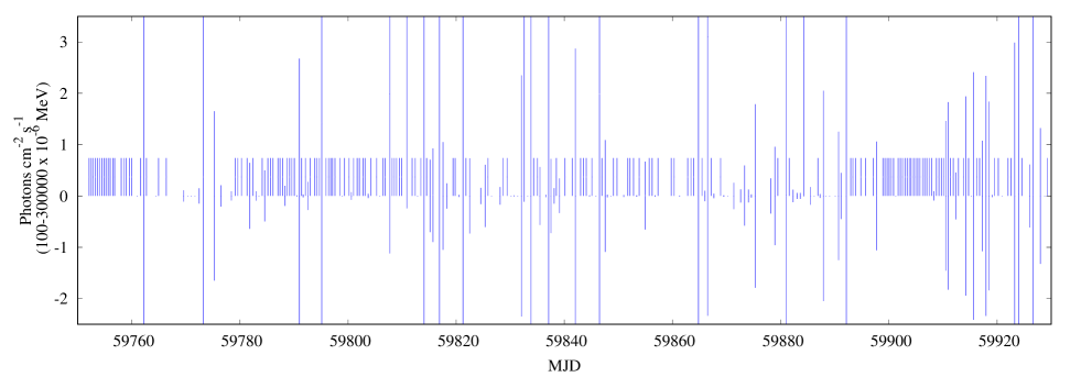
Figure 1: The figure represents the $\gamma$-ray light curve of Sag A* in the $\gamma$-ray band at a 3$\sigma$ confidence level from 2022 June 22 up to 2022 December 19 with a record of 180 days.

III Methods

III.1 Periodogram and Window Function

Following the data processing, an analysis was conducted to search for periodic patterns. To accomplish this, the R-package RobPer proved to be a valuable tool, enabling the examination of associated periodograms over extended time scales, spanning several years. This package was specifically developed for the analysis of astrophysical time series as discussed by Thieler, Rathjens, and Fried (2014).

RobPer operates by robustly fitting periodic functions to the given time series, typically in the form of light curves. It calculates periodograms even when observations are irregular and not evenly spaced in time. The RobPer identify significant peaks using various statistical techniques, as described by Thieler, Rathjens, and Fried (2014, and references therein). These techniques include options like least squares, least absolute deviations, least trimmed squares, M-, S-, and $\tau$ regression, and account for measurement accuracies by assigning weights to data points.

As mentioned by Thieler, Rathjens, and Fried (2014), one of the distinguishing features of RobPer is its ability to encompass different regression models, introducing flexibility in the analysis. In the search of critical values, it uses an outlier search to identify valid periods. This approach recognises that traditional assumptions may not always hold and aims to identify periodicities in a more robust manner. It is a susceptible to the influence of outliers, making it a robust method, inclusive to significant fluctuations.

For our case study of the $\gamma$-ray datasample of Sag A*, periodogram bars were computed by employing a two-step model-fitting approach, and the unweighted $\tau$-regression method was applied.

To enhance the reliability of the detected periods in the RobPer periodogram analysis and to mitigate the risk of false positives, we implemented a windowing program inspired by the methodology outlined in the work of Dawson and Fabrycky (2010).

With this Window Function we can differentiates between aliases and positive falses. This method is represented as $|f\pm f_{s}|$, where $f$ denotes the frequency of interest, and $f_{s}$ corresponds to a feature in the window function. To discern between aliases and true frequencies, a comparison is made between the phase and amplitude of expected aliases, generated from a sinusoidal waveform with the candidate frequency, and the data. By evaluating whether the predicted aliases align with the data in terms of amplitude, phase, and pattern, it becomes possible to ascertain the presence of the true period. When all aliases exhibit consistency in terms of these characteristics, we can confidently conclude that the genuine period has been successfully identified.

Therefore, the spectral Window Function of a regularly spaced time series is defined as follows (Magallanes-Guijón and Mendoza, 2022):

$$W(\nu)=\frac{1}{N}\sum_{r=1}^{N}e^{-2\pi i\nu t_{r}}$$ (1)

where the total number of data points is $N$, the time of the $r$-th is $t_{r}$ and data point $m$ is an integer. The peaks are observed at frequencies of $mf_{s}$.

In this approach, false positives are effectively eliminated through a direct comparison between a diagram of $W(\nu)$ vs $\nu$ (where $W(\nu)$ represents the spectral Window Function) and the periodograms generated using RobPer. This comparison allows for the identification of false positive periodicities within the dataset. For instance, if there is a spurious periodicity in the data caused by external factors, such as an annual cycle due to vacation days when no observations were made, it would manifest as a peak in the window function (WF). Figure 2 illustrates the periodograms produced with RobPer along with their respective time window functions for further clarity and validation.

IV Discussion

Figure 2 shows two prominent peaks in the light curve corresponding to $0.033$ d ($47.52$ min) and $0.053$ d ($76.32$ min). The peak at $0.053$ d ($76.32$ min) corresponds to a minimum in the WF and the peak at $0.033$ d ($47.52$ min) has a maximum in the WF. Therefore it is very likely that the $47.52$ min peak is a false positive and as such, a true single periodicity well defined at $76.32$ min with a strong peak on its light curve is very likely to occur.

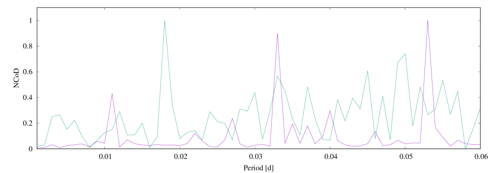
Figure 2: The magenta curve represents the $\gamma$-ray periodogram of the data sample of Figure 1 produced with RobPer and represented by their Normalised Coefficient of Determination (NCoD), with its corresponding normalised Window Function (green line). The strongest peak at $0.053$ d ($76.32$ min) is very likely due to a periodicity on the signal since it corresponds to a minimum on its Window Function.

The periodicity found in this work is very similar to two other periodicities:

• At millimetre wavelengths using the Atacama Large Millimiter/submillimeter Array (ALMA), Wielgus et al. (2022) studied the polarised light curves of Sgr A* and (Event Horizon Telescope Collaboration, 2022) reported a rotation in the electric vector position angle a timescale of $74\pm 6$ min as a signature of the orbital motion of a hot spot embedded in a magnetic field.

• An X-ray periodicity of about $149$ min in Sgr A* was reported by Leibowitz (2018). This periodicity is about two times the one found in this work, so it is quite possible this X-ray periodicity represents a harmonic of our $76.32$ min periodicity.

The coincidence of the multiwavelength periodicity in millimitre, X-ray and $\gamma$-ray points towards a single physical mechanism that produce it.

V Conclusions

Using the Fermi database, we have constructed the light curve of Sgr A* in $\gamma$-rays with a $3\sigma$ confidence level from 2022 June 22 up to 2022 December 19. We constructed its associated periodogram using RobPer. To avoid any false positive peaks in the periodogram, we compared any found peak with its Window Function. As a result, we found a $76.32$ min in the $\gamma$-ray lightcurve.

This periodicity is very close to that reported by Wielgus et al. (2022), and it is quite similar to a half of the one reported by Leibowitz (2018), suggesting the latter to be a harmonic of the $\sim\!76$ minutes. As such, all these periodicities point to the same physical mechanism as the one described by Wielgus et al. (2022), in which a blob of magnetised matter orbits about the central supermassive black hole in Sag A*.

References

- Balick and Brown (1974) Balick, B.and Brown, R. L., apj 194, 265 (1974).
- Boehle et al. (2016) Boehle, A., Ghez, A. M., Schödel, R., Meyer, L., Yelda, S., Albers, S., Martinez, G. D., Becklin, E. E., Do, T., Lu, J. R., Matthews, K., Morris, M. R., Sitarski, B., and Witzel, G., apj 830, 17 (2016), arXiv:1607.05726 [astro-ph.GA] .
- Boyce et al. (2019) Boyce, H., Haggard, D., Witzel, G., Willner, S. P., Neilsen, J., Hora, J. L., Markoff, S., Ponti, G., Baganoff, F., Becklin, E. E., Fazio, G. G., Lowrance, P., Morris, M. R., and Smith, H. A., apj 871, 161 (2019), arXiv:1812.05764 [astro-ph.HE] .
- Cabrera et al. (2013) Cabrera, J. I., Coronado, Y., Benítez, E., Mendoza, S., Hiriart, D., and Sorcia, M., MNRAS 434, L6 (2013), arXiv:1212.0057 [astro-ph.HE] .
- Cafardo, Nemmen, and Fermi LAT Collaboration (2021) Cafardo, F., Nemmen, R., and Fermi LAT Collaboration,, apj 918, 30 (2021), arXiv:2107.00756 [astro-ph.HE] .
- Dawson and Fabrycky (2010) Dawson, R. I.and Fabrycky, D. C., Astrophys. J. 722, 937 (2010), arXiv:1005.4050 [astro-ph.EP] .
- Event Horizon Telescope Collaboration (2022) Event Horizon Telescope Collaboration,, ApJL 930, L12 (2022).
- Fazio et al. (2018) Fazio, G. G., Hora, J. L., Witzel, G., Willner, S. P., Ashby, M. L. N., Baganoff, F., Becklin, E., Carey, S., Haggard, D., Gammie, C., Ghez, A., Gurwell, M. A., Ingalls, J., Marrone, D., Morris, M. R., and Smith, H. A., The Astrophysical Journal 864, 58 (2018).
- Genzel, Eisenhauer, and Gillessen (2010) Genzel, R., Eisenhauer, F., and Gillessen, S., Reviews of Modern Physics 82, 3121 (2010), arXiv:1006.0064 [astro-ph.GA] .
- Ghez et al. (2008) Ghez, A. M., Salim, S., Weinberg, N. N., Lu, J. R., Do, T., Dunn, J. K., Matthews, K., Morris, M. R., Yelda, S., Becklin, E. E., Kremenek, T., Milosavljevic, M., and Naiman, J., apj 689, 1044 (2008), arXiv:0808.2870 [astro-ph] .
- GRAVITY Collaboration et al. (2019) GRAVITY Collaboration,, Abuter, R., Amorim, A., Bauböck, M., Berger, J. P., Bonnet, H., Brandner, W., Clénet, Y., Coudé Du Foresto, V., de Zeeuw, P. T., Dexter, J., Duvert, G., Eckart, A., Eisenhauer, F., Förster Schreiber, N. M., Garcia, P., Gao, F., Gendron, E., Genzel, R., Gerhard, O., Gillessen, S., Habibi, M., Haubois, X., Henning, T., Hippler, S., Horrobin, M., Jiménez-Rosales, A., Jocou, L., Kervella, P., Lacour, S., Lapeyrère, V., Le Bouquin, J. B., Léna, P., Ott, T., Paumard, T., Perraut, K., Perrin, G., Pfuhl, O., Rabien, S., Rodriguez Coira, G., Rousset, G., Scheithauer, S., Sternberg, A., Straub, O., Straubmeier, C., Sturm, E., Tacconi, L. J., Vincent, F., von Fellenberg, S., Waisberg, I., Widmann, F., Wieprecht, E., Wiezorrek, E., Woillez, J., and Yazici, S., Astronomy and Astrophysics 625, L10 (2019), arXiv:1904.05721 [astro-ph.GA] .
- Leibowitz (2018) Leibowitz, E., MNRAS 474, 3380 (2018), arXiv:1711.04687 [astro-ph.HE] .
- Magallanes-Guijón and Mendoza (2022) Magallanes-Guijón, G.and Mendoza, S., arXiv e-prints , arXiv:2210.15884 (2022), arXiv:2210.15884 [astro-ph.HE] .
- Magallanes-Guijón (2020) Magallanes-Guijón, G., “Fermi-Tools Workshop: Light Curves,” (2020).
- Thieler, Rathjens, and Fried (2014) Thieler, A. M., Rathjens, J., and Fried, R., The RobPer-package (2014), r package version 1.2.
- Wielgus et al. (2022) Wielgus, M., Moscibrodzka, M., Vos, J., Gelles, Z., Martí-Vidal, I., Farah, J., Marchili, N., Goddi, C., and Messias, H., Astronomy and Astrophysics 665, L6 (2022), arXiv:2209.09926 [astro-ph.HE] .