A study for the energy structure of the Mott system with a low-energy excitation, in terms of the pseudo-gap in HTSC.

Abstract

The Mott system with a low-energy excitation may well constitute the underlying system for high temperature superconductivity (HTSC) of under-doped cuprates. This paper explores the above through the Hubbard-1 approximation (the Green function method), especially in terms of its self-energy. Results show it appears the pseudo-gap of HTSC is due to the self-energy effect on a quasi-particle excitation of $\sim 4t^{2}/U$ per two electrons, which is the Mott’s $J$.

I Introduction

The research objective of this study is to evaluate a strongly-correlated electron system near the Mott insulating state, the half-filled system, as the basis for high-temperature superconductivity (HTSC) of under-doped cuprates.

The mechanism of HTSC has remained unknown and is considered to be different from that of the BCS theory. For instance, the superconducting state of HTSC cuprates appears near the Mott insulators, and possess two types of energy-gaps (a superconductivity-gap and a pseudo-gap) reference4 ; reference5 ; reference6 ; reference7 ; reference8 under the Fermi surface reconstruction reference9 ; reference10 ; reference11 , as have been observed in spectroscopic experiments such as STS and ARPES. On the other hand, many researchers have proposed the occurrence of a low-energy excitation near this half-filled, such as due to spin-fluctuation reference12 ; reference13 , density-wave reference14 ; reference15 , spin-charge separation reference16 , two-component fermion reference17 , and multi orbital effects reference18 ; reference19 .

In light of the above, the Mott system with a low-energy excitation seems to be well suited to representing the underlying system of HTSC cuprates. Therefore, an investigation of this system may afford a new insight into the physical phenomena of HTSC cuprates and hopefully other unconventional superconductors reference20 ; reference21 ; reference22 .

First, this paper presents the effective Hamiltonian for the Hubbard model with a low-energy excitation, in order to provide the concept of this subject, and second, investigates it using the Hubbard-1 approximation (non-interacting single-particle Green function method) reference3 reference27 ; reference28 ; reference29 ; reference30 ; reference31 , which represents electron systems incorporating self-energy near the Mott system, and third, evaluates the theoretical values of this model through the experimental values of Bi2212s, while verifying the resulting self-energy effect with the effective-mass at $T=0K$, in order to clarify the origin of the pseudo-gap in HTSC.

Typically, the Hubbard-1 approximation first finds the self-energy at the atomic limit, and then considers dispersion relations $\epsilon(\textbf{k})$ (including $t$), when expanding into a band structure reference30 ; reference31 . In contrast, this paper incorporates a particular excitation of the Mott system into the approximation, instead of $\epsilon(\textbf{k})$. This excitation ($\Delta_{J}$) is assumed to appear at [0, $\pi$] and [$\pi$, 0] in $k$-space (reciprocal lattice space) in HTSCs reference7 and be some quasi-particle excitation related to an antiferromagnetic interaction, $J$ ($\sim 4t^{2}/U$) of the Mott system.

II Effective Hamiltonian

The effective Hamiltonian ($H_{eff}$) for the Mott system with a low-energy excitation is shown as follows, which does not include the self-energy effect of this system.

$$H_{eff} = H_{kinetic}+H_{potential}+H_{coulomb-energy}.$$ (1a)

$$= -t\sum_{<i,j>\sigma}\left(c^{\dagger}_{r_{i}\sigma}c_{r_{j}\sigma}+c^{\dagger}_{r_{j}\sigma}c_{r_{i}\sigma}\right)$$

$$+ \gamma\sum_{<i,j>\sigma}\left(c^{\dagger}_{r_{i}\sigma}c_{r_{i}\sigma}+c^{\dagger}_{r_{j}\sigma}c_{r_{j}\sigma}\right)$$

$$+ U\sum_{(i)}^{N}n_{i\uparrow}n_{i\downarrow}.$$

$$\gamma = 0~{}~{}or~{}~{}\Delta_{J}.$$ (1b)

$$2\Delta_{J} = (1/2)\sum_{(l)}~{}\Delta_{J}~{}|cos(k_{x})-cos(k_{y})|.$$ (1c)

$$l = [k_{x},k_{y}]=[0,\pi]~{}and~{}[\pi,0].$$ (1d)

where $t$ is the transfer integral, $U$ is the coulomb repulsion (Mott gap), and $\Delta_{J}$ is an assumed low-energy excitation per electron, where $U/t=8$ and $U=3.2~{}eV$. $r_{i}\sigma$ and $r_{j}\sigma$ represent a pair of nearest-neighbor sites with spin $\sigma(=\uparrow or\downarrow)$, $n$ is the spin-density operator. The coefficient $\gamma$ of the second term in Eq(Equation). (1a) has a value of either $0$ or $\Delta_{J}$, which is a quasi-particle excitation (a quasi-particle level) specific to the Mott system. The occupancy ratio $\nu$ is considered to be 1 here. The self-energy effect of this system shifts $\Delta_{J}$ into $\delta$ as demonstrated in Section 3.

III Green function

III.1 Green function

The physical properties based on the above Hamiltonian are investigated through the Green function method as described below reference3 reference30 ; reference31 . The calculation of the Green function and the self-energy is divided into two spectra, that is, $G^{R}_{1}(\textbf{}\omega)$ and $\Sigma^{R}_{1}(\textbf{}\omega)$ per electron, which are independent of k reference30 , as well as $G^{R}_{2}(\textbf{}\omega)$ and $\Sigma^{R}_{2}(\textbf{}\omega)$ per electron, which relates to an additional self-energy caused by $\Delta_{J}$.

The following Green functions build on the thermal average of the number of particles. But it is assumed that what an electron hops into the $\Delta_{J}$ level is possible even at lower temperatures than that of thermal excitation, as a quasi-particle excitation with a finite lifetime.

III.2 Single-particle Green function

The single-particle Green functions ($G^{R}(\omega)$) of the Hubbard model with a low-energy excitation at the atomic limit is shown as follows.

$$G^{R}(\omega) = G^{R}_{1}(\textbf{}\omega)+G^{R}_{2}(\textbf{}\omega).$$ (2a)

$$G^{R}_{1}(\textbf{}\omega) = \frac{1-<n_{-\sigma,\bar{\Delta_{J}}}>}{\omega+\mu^{{}^{\prime}}-0}+\frac{<n_{-\sigma,\bar{\Delta_{J}}}>}{\omega+\mu^{{}^{\prime}}-U}.$$ (2b)

$$G^{R}_{2}(\textbf{}\omega) = \frac{1-<n_{-\sigma,\Delta_{J}}>}{\omega+\mu^{{}^{\prime}}-\Delta_{J}}+\frac{<n_{-\sigma,\Delta_{J}}>}{\omega+\mu^{{}^{\prime}}-U}.$$ (2c)

$$\mu^{{}^{\prime}} = 0.$$ (2d)

$$~{}<n_{-\sigma,\bar{\Delta_{J}}}> + <n_{-\sigma,\Delta_{J}}>=\nu$$ (2e)

And also,

$$\textless n_{-\sigma,~{}x}\textgreater = \nu f(x).~{}~{}~{}~{}~{}~{}~{}~{}~{}$$ (3a)

$$\textless n_{-\sigma,~{}\bar{x}}\textgreater = \nu(1-f(x)).~{}~{}$$ (3b)

$$f(x) = \frac{1}{1+e^{(\beta x)}}~{}~{}$$ (3c)

$$\nu f(x)+\nu(1-f(x)) = \nu$$ (3d)

where $\mu$ ($\mu{{}^{\prime}}$ and $\mu^{{}^{\prime\prime}}$) is the chemical potential, $\Delta_{J}$ is the original low-excitation per electron, $\nu$ is the occupation ratio, which is equal to ”1 minus the hole concentration” and has a range of $0.7<\nu<1$ in this under-doped study, $f(x)$ is the modified Fermi-Dirac distribution function in which $x$ itself represents the energy difference from the chemical potential (Fermi-level), $\beta=1/kT$, and $\textless n_{-\sigma,x}\textgreater$ (weighting factor) is the thermal average of the density of opposite-spin particles as the nearest-neighbors. The number of sites per energy-level is 1 and double occupancy is not allowed, so that the combination of $\textless n_{-\sigma,\bar{x}}\textgreater$ and $\textless n_{-\sigma,x}\textgreater$ satisfies $\textless n_{-\sigma,\bar{x}}\textgreater+\textless n_{-\sigma,x}\textgreater=1\times\nu$ at finite temperature.

The chemical potential in a hole-doped region ($\nu<1$) lies at the top of the lower-band (valence band) at this step. Note that the chemical potential at the half-filled ($\nu=1$) rises to the center of the energy-gap as a feature of the Mott system.

In this model, a free electron of these Green functions is assumed to be subject to the same restrictions as that on a doped CuO₂ plane, hopping from one of the nearest-neighbor sites under the antiferromagnetic condition to either a vacancy site ($1-\textless n_{-\sigma,x(~{}or~{}\bar{x})}\textgreater$) or an opposite-spin site ($\textless n_{-\sigma,x(~{}or~{}\bar{x})}\textgreater$, single occupied state) at the energy-level $0$ or $\Delta_{J}$. When it is added to an opposite-spin site and then hopped back, the energy of this system increases to $U$ for a moment.

III.3 Self-energy

The self-energy of the atomic limit ($\Sigma^{R}(\omega)$) based on the above Green functions is shown as follows, through the Dyson equation.

$$\Sigma^{R}(\omega) = \Sigma^{R}_{1}(\textbf{}\omega)+\Sigma^{R}_{2}(\textbf{}\omega).$$ (4a)

$$\Sigma^{R}_{1}(\textbf{}\omega) = U<n_{-\sigma,\bar{\delta}}>+0\times(1-<n_{-\sigma,\bar{\delta}}>)$$ (4b)

$$+ U^{2}\times\frac{<n_{-\sigma,\bar{\delta}}>(1-<n_{-\sigma,\bar{\delta}}>)}{\omega+\mu^{{}^{\prime}}+0-U(1-<n_{-\sigma,\bar{\delta}}>)}.$$

$$\Sigma^{R}_{2}(\textbf{}\omega) = U<n_{-\sigma,\delta}>+\Delta_{J}(1-<n_{-\sigma,\delta}>)$$

$$+(U-\Delta_{J})^{2} \times \frac{<n_{-\sigma,\delta}>(1-<n_{-\sigma,\delta}>)}{\omega+\mu^{{}^{\prime}}-\Delta_{J}<n_{-\sigma,\delta}>-U(1-<n_{-\sigma,\delta}>)}.$$

$$\mu^{{}^{\prime}} = 0.$$ (4d)

$$<n_{-\sigma,\bar{\delta}}> + <n_{-\sigma,\delta}>=\nu$$ (4e)

where $\delta$ is a quasi-particle spectral gap that is produced from Eq. (6a) and is self-consistently determined through Eqs. (4a)-(4e) and Eqs. (6a)-(6c) as these equations are in an equilibrium state. $\Sigma^{R}_{2}(\textbf{}\omega)$ is a constant at $T=0~{}K$.

III.4 Hubbard-1 approximation

The spectrum of the Hubbard-1 approximation ($G^{R}_{H1}(\omega)$) with the self-energy is shown as follows.

$$G^{R}_{H1}(\mathbf{k},\omega) = \frac{1-\textless n_{-\sigma,\bar{\delta}}\textgreater}{\omega+\mu^{{}^{\prime\prime}}-0-\epsilon(\mathbf{k})-\Sigma^{R}_{1}(\omega)}.$$ (5a)

$$+ \frac{1-\textless n_{-\sigma,\delta}\textgreater}{\omega+\mu^{{}^{\prime\prime}}-\Delta_{J}-(\Sigma^{R}_{1}(\omega)+\Sigma^{R}_{2}(\omega))}.$$

At $\textbf{k}=\textbf{k}_{F}$ ($\epsilon(\textbf{k}_{F})=0$) in the first term,

$$G^{R}_{H1}(\omega) = \frac{1-\textless n_{-\sigma,\bar{\delta}}\textgreater}{\omega+\mu^{{}^{\prime\prime}}-0-\Sigma^{R}_{1}(\omega)}.$$ (6a)

$$+ \frac{1-\textless n_{-\sigma,\delta}\textgreater}{\omega+\mu^{{}^{\prime\prime}}-\Delta_{J}-(\Sigma^{R}_{1}(\omega)+\Sigma^{R}_{2}(\omega))}.$$

$$\mu^{{}^{\prime\prime}} = \Sigma^{R}_{1}(\omega=0).$$ (6b)

$$\textless n_{-\sigma,\bar{\delta}}\textgreater + \textless n_{-\sigma,\delta}\textgreater=\nu$$ (6c)

where $\epsilon(\textbf{k})$ is a dispersion relation across the entire k, and $\textbf{k}_{F}$ is the wave vector at the Fermi-level. The first term creates a pole at the Fermi-level and the second term creates a pole ($+\delta$) above the Fermi-level. The chemical potential is set to $\mu^{{}^{\prime\prime}}=\Sigma^{R}(\omega=0)$. The additional self-energy $\Sigma^{R}_{2}(\textbf{}\omega)$ is assumed to overlap the local self-energy $\Sigma^{R}_{1}(\textbf{}\omega)$ at $\Delta_{J}$.

IV Results

The study of the Hubbard model with a low-energy excitation through the Green function methods in this paper shows the following results. This investigation focuses on the energy spectra of the Fermi-level ($\epsilon(\textbf{k}_{F})=0$) and $\delta$ at [0,$\pi$] or [$\pi$,0] in k-space, using $G^{R}(\omega)$ (Gray lines, thereafter) in Eq. (2a) and $G^{R}_{H1}(\omega)$ (Red lines, thereafter) in Eq. (6a), the latter of which shifts an original excitation $\Delta_{J}$ into a spectral gap $\delta$ of the Green function through the self-energy effect of this system.

Setting its original excitation as $\Delta_{J}=0.1~{}eV$ results in a spectral gap $\delta=0.038~{}eV$ as shown in Fig(Figure).1, where $\nu=0.8$, $T=0K$, $U=3.2~{}eV$, and $U/t=8$. The relation between $\Delta_{J}$ - $\delta$ near $\Delta_{J}=0.1~{}eV$ is shown in Fig.2, with the same $\nu$, $T$, and $U/t$ as the above : ($\Delta_{J}$[$eV$], $\delta$[$eV$]) = (0.075, 0.029), (0.1, 0.038), and (0.125, 0.047).

The size of $\delta$ is also dependent on an occupation ratio $\nu$ and/or slightly temperature $T$ as shown in Figs.1,3-5 : ($\nu$, $T$[$K$], $\delta$[$eV$]) = (0.8, 0, 0.038), (0.9, 0, 0.019), (0.7, 0, 0.058), and (0.8, 100, 0.040).

Besides, Fig.6 shows the wider range of the spectral curves for Fig.1 with $\nu=0.8$, $T=0~{}K$, $\Delta_{J}=0.1~{}eV$ and $U/t=8$, in which the poles of $G^{R}_{H1}(\omega)$ appear at 0, 0.038, 3.2, and 3.36 $eV$. Fig.7 shows the relation between occupancy ratios and the sizes of $\delta$s.

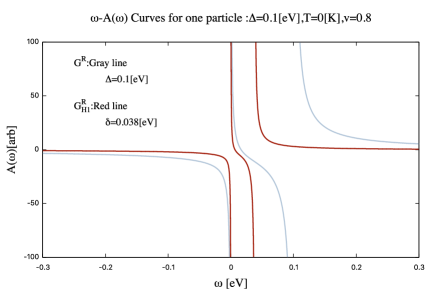
Figure 1: $\omega-G(\omega$) (indicated as $A(\omega$) in the figure) curves for one particle: Gray ($G^{R}(\omega)$) denotes the Green function not including self-energy, Red ($G^{R}_{H1}(\omega)$) denotes that including self-energy. $|\delta|\sim 0.038~{}eV$ ($2\delta\sim 0.076~{}eV$), when $\nu=0.8$, $T=0~{}K$, $\Delta_{J}=0.1~{}eV$, and $U/t=8$.

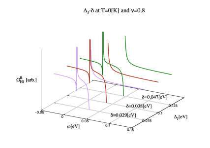
Figure 2: $\Delta_{J}-\delta$: ($\Delta_{J}$[$eV$], $\delta$[$eV$]) = (0.075, 0.029), (0.1, 0.038) and (0.125, 0.047), where $\nu=0.8$, $T=0~{}K$, and $U/t=8$.

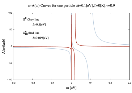
Figure 3: $\omega-G(\omega$) curves for one particle: $|\delta|\sim 0.019~{}eV$, when $\nu=0.9$, $T=0~{}K$, $\Delta_{J}=0.1~{}eV$, and $U/t=8$. Refer to Fig. 1.

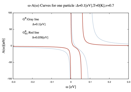
Figure 4: $\omega-G(\omega$) curves for one particle: $|\delta|\sim 0.058~{}eV$, when $\nu=0.7$, $T=0~{}K$, $\Delta_{J}=0.1~{}eV$, and $U/t=8$. Refer to Fig. 1.

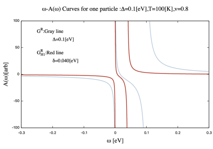
Figure 5: $\omega-G(\omega)$ curves for one particle: $|\delta|\sim 0.040~{}eV$, when $\nu=0.8$, $T=100~{}K$, $\Delta_{J}=0.1~{}eV$, and $U/t=8$. $\mu^{"}$ is assumed to be the same as that at $T=0~{}K$. Refer to Fig. 1.

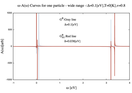
Figure 6: $\omega-G(\omega$) curves for one particle (Wide range): $|\delta|\sim 0.038~{}eV$, when $\nu=0.8$, $T=0~{}K$, $\Delta_{J}=0.1~{}eV$, and $U/t=8$. The poles of $G^{R}(\omega)$ are 0, 0.1, and 3.2 $eV$. The poles of $G^{R}_{H1}(\omega)$ are 0, 0.038, 3.2, and 3.36 $eV$. Refer to Fig.1.

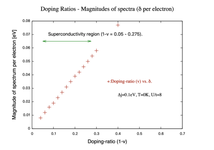
Figure 7: Doping-ratios - Magnitudes of spectral gaps ($\delta$ per electron), where $T=0K$, $\Delta_{J}=0.1~{}eV$, and $U/t=8$.

IV.1 Effective mass

The effective-mass ratio is expressed as $m^{*}/m=1/Z$ at $T=0~{}K$, where Z is the quasi-particle renormalization factor as follows reference23 , because of a discontinuity of the momentum distribution at $\textbf{k}=\textbf{k}_{F}$ and $T=0~{}K$.

$$m^{*}/m = 1/Z~{}~{}~{}\mbox{($T=0~{}K$)}$$ (7a)

Z $$= [1-\partial Re\Sigma^{R}_{1}(\omega)/\partial\omega]^{-1}|_{\textbf{k}=\textbf{k}_{F},\omega=0^{+}}.$$ (7b)

The effective-mass ratio $m^{*}/m$ of this model varies $3-10$ at $T=0~{}K$ as the occupation ratio $\nu$ varies $0.7-0.9$, a region in a superconducting state of HTSCs reference7 , to which the Fermi liquid theory can be applied, shown in Fig. 8, where $\Delta_{J}=0.1~{}eV$ and $U/t=8$ : ($\nu$, $m^{*}/m$)= (0.9, 10), (0.8, 5), (0.7, 3.3), (0.6, 2.5), and (0.5, 2.0). The effective-mass ratio depends on $\nu$ (not $\Delta_{J}$) at $T=0~{}K$.

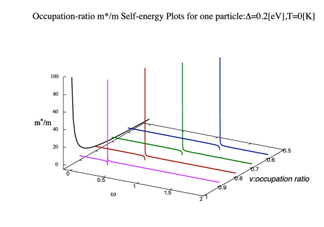
Figure 8: Occupation ratios ($\nu$) - Effective-mass ratio ($m^{*}/m$) curve for one particle: The effective-mass ratio $m^{*}/m$ varies $2-10$ at $T=0~{}K$ as the occupation ratio $\nu$ varies $0.5-0.9$, where $\omega=0^{+}$, $T=0~{}K$, $\Delta_{J}=0.1~{}eV$, and $U/t=8$.

V Discussion

This section verifies the above results derived from the model of this paper, using the past experimental results. It is assumed that Bi2212 should have the pseudo-gap of $\sim 0.04~{}eV$ (per electron) as its maximum value at the occupancy ratio $\nu=0.8$ and $T=0~{}K$ reference7 .

First, when an original excitation is set as $\Delta_{J}=0.1~{}eV$ (per electron), the resulting spectral gap $\delta\sim 0.038~{}eV$ (per electron) at $\nu=0.8$ and $T=0~{}K$ appears. Notably, the magnitude of $0.1eV$ (per electron) is on the order of the exchange interaction constant $J$ of the Mott system when $t=0.4eV$ and $U=3.2eV$, that is $J=4t^{2}/U=0.2eV=2\Delta_{J}$ (per two electrons).

In addition, both the occupancy-ratio dependence and the temperature dependence of the size of $\delta$ are also similar to what are expected from the experiments of Bi2212. The higher the temperature or the smaller the occupation ratio is, the larger the size of $\delta$ is. As the occupation ratio approaches zero, the size of $\delta$ approaches $\Delta_{J}$, and when the occupation ratio is unity, $\delta$ vanishes.

However, upon closer inspection, whereas in experiments, the relation between occupancy ratios and the sizes of pseudo-gaps depicts a dome shape, in this model, the relation between those is linear as shown in Fig.7.

Second, the effective mass of this model is in good agreement with the experimental results of HTSCs reference24 ; reference25 ; reference26 . In particular, the effective-mass ratio $m^{*}/m$ of this model varies from 3 to 10 at $T=0~{}K$ as the occupation ratio $\nu$ varies from 0.7 to 0.9. This is because, as the occupation ratio decreases and/or temperature increases, the pole of the self-energy of this system moves upward from the Fermi-level to $U$, and accordingly the rate of change in the self-energy decreases at the Fermi-level.

Note that Fig.9 shows the gap of $\delta$ in the $\omega-G(\omega$) curves becomes symmetric with respect to the chemical potential, when it is taken as $\mu^{{}^{\prime\prime}}=\Sigma^{R}_{1}(\omega=0)+\Sigma^{R}_{2}(\omega=0)$ in Eq. (6b).

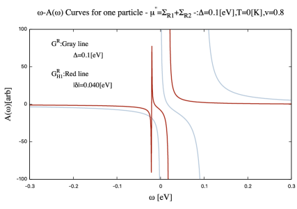
Figure 9: $\omega-G(\omega$) curves for one particle: Gray ($G^{R}(\omega)$) denotes the poles of the Green function not including self-energy, Red ($G^{R}_{H1}(\omega)$) denotes those including self-energy. The chemical potential $\mu^{{}^{\prime\prime}}=\Sigma^{R}_{1}(\omega=0)+\Sigma^{R}_{2}(\omega=0)$. $|\delta|\sim 0.040~{}eV$ ($2\delta\sim 0.080~{}eV$), when $\nu=0.8$, $T=0~{}K$, $\Delta_{J}=0.1~{}eV$, and $U/t=8$.

VI Conclusions

This paper has constructed the underlying model for HTSC cuprates in the under-doped region, that is, a Mott electron system with a low-energy excitation, and investigated its gap spectra in terms of self-energy, while evaluating the calculation of self-energy using effective mass ratio. This model incorporates an additional self-energy at $\textbf{k}^{{}^{\prime}}=(0,\pi)|(\pi,0)$, in addition to the self-energy across the entire k.

The results suggest the pseudo-gap of HTSC is considered to be due to the self-energy effect on a quasi-particle excitation of the Mott system, and the energy order of this excitation is $J$ ($\sim 4t^{2}/U$) per two electrons.

It is quite possible that the excitation of $4t^{2}/U$ appears in this system, since $4t^{2}/U$ is the energy of quadruple degenerate second-order perturbation in the Mott system, which is the origin of its magnetism. Furthermore, the self-energy estimate appears to be adequate with respect to its effective mass ratio. The effective mass is calculated from the self-energy at $\omega=0$.

Concerning the effective-mass ratio, it also suggests the underlying system of HTSC evolves from an insulator, and through the suppression of self-energy, behaves as a Fermi liquid in the optimal-doping region.

It follows from the above that, the underlying system of HTSC is depicted as the Fermi liquid state, with a low-energy excitation, that activates antiferromagnetic correlations while being enveloped in a cloud of self-energy, both of which, that is, antiferromagnetic correlation and self-energy are inherent in the Mott system in the under-doped region.

At last, the possibility of the equivalence between the pseudo-gap of HTSC and the Mott’s J derived from this study may contribute to the elucidation of superconductivity in hole-doped cuprates.

VII The Bibliography

References

- (1) J.Bardeen, L.N.Cooper, J.R.Schrieffer, Phys.Rev. (1957).
- (2) N.F.Mott, Rev.Mod.Phys.40,677 (1968).
- (3) Hubbard,J.(1963). Proceedings of the Royal Society A 276 (1365): 238.
- (4) T.Timusk, and B. Statt, Rep.Prog. Phys.62,61(1999).
- (5) Kiyohisa.Tanaka, W.S.Lee, D.H.Lu, A.Fujimori, T.Fujii, Risdiana, I.Terasaki, D.J.Scalapino, T.P.Devereaux, Z.Hussain, and Z.-X.Shen, Science 314, 1910-1913 (2006).
- (6) T.Kondo, T.Takeuchi, A.Kaminski, S.Tsuda, and S.Shin, Phys.Rev.Lett. 98 (2007) 267004.
- (7) W.S. Lee, I.M. Vishik, K.Tanaka, D.H.Lu, T.Sasagawa, N.Nagaosa, T.P.Devereaux, Z. Hussain, Z.-X. Shen, Nature 450, 81-84 (2007)
- (8) Ch.Renner, B.Revaz, J.-Y. Genoud, K.Kadowaki, and O.Fischer, Phys.Rev.Lett. 80,149 (1998).
- (9) M.R.Norman, H.Ding, M.Randeria, J.C.Campuzano, T.Yokoya, T.Takeuchi, T.Takahashi, T.Mochiku, K.Kadowaki, P.Guptasarma, and D.G.Hinks, Nature 392, 157 (1998).
- (10) M.Hashimoto, R.-H.He, K.Tanaka, J.P.Testaud, W.Meevasana, R.G.Moore, D.-H.Lu, H.Yas, Y.Yoshida, H.Eisaki, Z.Hussain, and Z.-X.Shen, Nat.Physics 6, 414 (2010).
- (11) H.-B.Yang, J.D.Rameau, Z.-H.Pan, G.D.Gu, P.D.Johnson, H.Claus, D.G.Hinks, and T.E.Kidd, Phys.Rev.Lett. 107, 047003 (2011).
- (12) P.Monthoux, A.V.Balatsky, and D.Pines, Rev.B.46(22),14803-14817 (1992).
- (13) K.Kurashima, T.Adachi, K.M.Suzuki, Y.Fukunaga, T.Kawamata, T.Noji, H.Miyasaka, I.Watanabe, M.Miyazaki, A.Koda, R.Kadono, and Y.Koike, Phys. Rev. Lett.121,057002
- (14) E.Demler, S.Sachdev, and Y.Zhang, Phys.Rev.Lett. 87, 067202 (2001).
- (15) B.Lake, G.Aeppli, K.N.Clausen, D.F.McMorrow, K.Lefmann, N.E.Hussey, N.Mangkorntong, M.Nohara, H.Takagi, T.E.Mason, and A.Schröder, Science 291,1759-1762 (2001).
- (16) M.Kohno, Phys.Rev.Lett.105 106402 (2010).
- (17) S Sakai, M.Civelli, and M.Imada, Phys.Rev.Lett.116, 057003 (2016)
- (18) H.Kontani and S.Onari, Phys.Rev.Lett.104,157001 (2010).
- (19) H.Sakakibara, K.Suzuki, H.Usui, S.Miyao, I.Maruyama, K.Kusakabe, R.Arita, H.Aoki, and K.Kuroki, Phys.Rev.B 89,224505 (2014)
- (20) Nagamatsu, J.; Nakagawa, N.; Muranaka, T.; Zenitani, Y.; Akimitsu, J. Nature 410: 63 (2001).
- (21) M.Hiraishi, S.Iimura, K.M.Kojima, J.Yamaura, H.Hiraka, K.Ikeda, P.Miao, Y.Ishikawa, S.Torii, M.Miyazaki, I.Yamauchi, A.Koda, K.Ishii, M.Yoshida, J.Mizuki, R.Kadono, R.Kumai, T.Kamiyama, T.Otomo, Y.Murakami, S.Matsuishi and H.Hosono, Nature physics,10, pages 300-303 (2014)
- (22) Y.Maeno, H.Hashimoto, K.Yoshida, S.Nishizaki, T.Fujita, J.G.Bednorz, and F.Lichtenberg, Nature 372,532 (1994)
- (23) R.Asgari, B.Davoudi, M.Polini, Gabriele F.Giuliani, M.P.Tosi, and G.Vignale: Phys.Rev. B71, 045323 (2005).
- (24) N. D. Leyraud, C. Proust, D. LeBoeuf, J. Levallois, J. B. Bonnemaison, R. Liang, D. A. Bonn, W. N. Hardy, L. Taillefer, Nature 447 (2007) 565.
- (25) S. E. Sebastian, N. Harrison, M. M. Altarawneh, C. H. Mielke, R. Liang, D. A. Bonn, W. N. Hardy, G. G. Lonzarich, Proc. Natl. Acad. Sci. 107 (2010) 6175.
- (26) J. Singleton, C. delaCruz, R. D. McDonald, S. Li, M. Altarawneh, P. Goddard, I. Franke, D. Rickel, C. H. Mielke, X. Yao, P. Dai, Phys. Rev. Lett. 104 (2010) 086403.
- (27) M.C.Gutzwiller: Phys.Rev.Lett.10,159 (1963).
- (28) F.C.Zhang and T.M.Rice: Phys.Rev.B37,3759 (1988).
- (29) L.F.Feiner, J.H.Jefferson, and R.Raimondi: Phys.Rev.B53,8751 (1996).
- (30) M.S.Laad, ”Local approach to the one-band Hubbard model: Extension of the coherent-potential approximation”, Phys.Rev.B 49(4), 2327-2330 (1994)
- (31) F. Gebhard, “The Mott Metal-Insulator Transition - Models and Methods”, No. 137 in Springer Tracts in Modern Physics (Springer, Heidelberg, 1997).