MALCOM-PSGD: Inexact Proximal Stochastic Gradient Descent for Communication-Efficient Decentralized Machine Learning

Abstract

Recent research indicates that frequent model communication stands as a major bottleneck to the efficiency of decentralized machine learning (ML), particularly for large-scale and over-parameterized neural networks (NNs). In this paper, we introduce Malcom-PSGD, a new decentralized ML algorithm that strategically integrates gradient compression techniques with model sparsification. Malcom-PSGD leverages proximal stochastic gradient descent to handle the non-smoothness resulting from the $\ell_{1}$ regularization in model sparsification. Furthermore, we adapt vector source coding and dithering-based quantization for compressed gradient communication of sparsified models. Our analysis shows that decentralized proximal stochastic gradient descent with compressed communication has a convergence rate of $\mathcal{O}\left(\ln(t)/\sqrt{t}\right)$ assuming a diminishing learning rate and where $t$ denotes the number of iterations. Numerical results verify our theoretical findings and demonstrate that our method reduces communication costs by approximately $75\%$ when compared to the state-of-the-art method.

1 Introduction

With the growing prevalence of computationally capable edge devices, there is a necessity for efficient learning algorithms that preserve data locality and privacy. One popular approach is decentralized ML. Under this regime, nodes within the network learn a global model by iterative model communication, whilst preserving data locality (Lalitha et al., 2018). It has been shown that decentralized ML algorithms can achieve similar accuracy and convergence rates to their centralized counterparts under certain network connectivity conditions (Nedic & Ozdaglar, 2009; Scaman et al., 2017; Koloskova et al., 2019; Lian et al., 2017). While decentralized ML eliminates the need for data uploading, (Bonawitz et al., 2019; Van Berkel, 2009; Li et al., 2020) observed that iterative model communication over rate-constrained channels creates a bottleneck. Particularly, the performance of decentralized training of large-scale deep neural network (DNN) models is substantially limited by excessively high communication costs (Chilimbi et al., 2014; Seide et al., 2014; Ström, 2015). This emphasizes the importance of designing efficient protocols for the communication and aggregation of high-dimensional local models.

Recent research has shown that efficiency of model communication can be enhanced by model sparsification and gradient/model compression. Model sparsification involves reducing the dimensionality of model parameters by exploiting their sparsity (Tan et al., 2011). On the other hand, model and gradient compression for decentralized ML has been studied in Alistarh et al. (2017); Koloskova et al. (2021; 2019); Han et al. (2015); Wen et al. (2017); Lin et al. (2018); Seide et al. (2014). It typically leverages lossy compression methods, such as quantization and source coding, to compress local model updates prior to communication. While this approach reduces communication bandwidth, it inevitably introduces imprecision during model aggregation.

Related Work. Kempe et al. (2003); Xiao & Boyd (2004); Boyd et al. (2006); Dimakis et al. (2010) proposed gossiping algorithms for consensus aggregation of local optimization results by leveraging peer-to-peer or neighborhood communication. Recently, Koloskova et al. (2019); Zhang et al. (2017); Scaman et al. (2017) adopted the gossiping algorithm for decentralized ML with convex and smooth loss functions, where convergence is guaranteed with constant and diminishing step sizes. Continuing this work, Koloskova et al. (2021); Lian et al. (2017); Nadiradze et al. (2021); Tang et al. (2018) generalized the approach to smooth but non-convex loss functions and provided convergence guarantees. Furthermore, (Koloskova et al., 2019) and (Tang et al., 2018) utilized gradient compression by compressing the model updates before communication and aggregation. Notably, Alistarh et al. (2017) proposed a dithering-based quantization scheme as well as a symbol-wise source coding method for ML model compression. Meanwhile, Nadiradze et al. (2021) analyzed the convergence of asynchronous decentralized optimization with model compression. While communication compression is advantageous in of itself, Alistarh et al. (2018); Stich et al. (2018) analytically and numerically demonstrated the bandwidth gains from gradient sparsfication.

Nesterov (2013) proposed proximal gradient descent (PGD) for the optimization of a non-smooth function with separable convex and smooth components. Subsequently, Beck & Teboulle (2009) studied the convergence of PGD when the proximal optimization step can be effectively executed via a soft-thresholding operation. Continuing this work, Schmidt et al. (2011) generalized the method for a convex objective with inexact gradient descent steps, while Sra (2012) established the convergence rate of inexact PGD for non-convex objectives. Meanwhile, in the decentralized convex optimization setting, Chen (2012) proved the convergence of inexact PGD with sub-optimal proximal optimization. Furthermore, Zeng & Yin (2018b) introduced general decentralized PGD algorithms and established the convergence rates for both constant and decreasing step sizes. However, to the best of our knowledge, the perturbations caused by data sub-sampling alongside stochastic gradient descent (SGD) updates and the lossy gradient compression have been overlooked in the literature.

Our Contributions. In this work, we address the challenge of enhancing the communication efficiency in compressed decentralized ML with a non-convex loss. We introduce the Multi-Agent Learning via Compressed updates for Proximal Stochastic Gradient Descent (Malcom-PSGD) algorithm, which communicates compressed and coded model updates. Our algorithm leverages model sparsification to reduce the model dimension by incorporating $\ell_{1}$ regularization during the SGD update. However, this non-smooth regularization term complicates the direct use of existing decentralized SGD algorithms in local training. In response, we introduce a strategy that combines decentralized proximal SGD to solve the regularized decentralized optimization, alongside gradient compression to alleviate the communication cost. Our findings suggest that the gradient quantization process introduces notable aggregation errors during the consensus step, making the conventional analytical tools on exact PGD inapplicable. We introduce an analytical framework to elucidate the influence of model compression on consensus aggregation and overall learning convergence. Furthermore, our theoretical analysis established the convergence rate of the proposed algorithm under decreasing SGD and consensus stepsizes. The contributions of this work are summarized as follows.

• We introduce a decentralized ML algorithm, Malcom-PSGD, by adopting the gossiping algorithm to coordinate local model communication and aggregation. To improve upon model compression, we promote model sparsity by optimizing an $\ell_{1}$ regularized training loss function on the local devices. Since this non-smooth optimization makes traditional decentralized SGD infeasible, we employ proximal SGD for local model update, together with residual (i.e., local model changes) compression via quantization and source coding methods. Furthermore, the proposed aggregation scheme merges the local model with its neighbor’s model prior to proximal optimization. Here, consensus and local updates find balance through the choice of the stepsize. In comparison to the existing decentralized SGD algorithm in (Koloskova et al., 2021), our consensus step boosts training convergence even without maintaining a constant average over iterations.

• We prove that Malcom-PSGD converges in the objective value for non-convex and smooth loss functions with a given quantization error. In particular, Malcom-PSGD exhibits a convergence rate of $\mathcal{O}(\ln{t}/\sqrt{t})$ and a consensus rate of $\mathcal{O}(1/t)$ with diminishing learning rates and consensus stepsizes, where $t$ represents the number of training rounds. Our convergence analysis quantifies the effects of mini-batch data sampling and lossy model compression on convergence.

• We employ the vector source coding scheme from Woldemariam et al. (2023) to further minimize communication requirements, by encoding the support vector of entries that match a certain quantization level. Our use of compressed model updates and differential encoding allows us to reasonably assume we are creating a structure within our updates that this encoding scheme is most advantageous under. This allows us to benefit from the compression under this scheme. We numerically demonstrate that our chosen scheme considerably reduces the communication bit requirement when compared to the existing model compression method in Alistarh et al. (2017).

We evaluate the performance of the proposed algorithm over various decentralized ML tasks. Numerical experiments demonstrate that our algorithm outperforms the state-of-the-art baseline, achieving a $75\%$ reduction in communication costs.

2 Decentralized Learning

We consider a decentralized learning system composed of $n$ nodes, whose goal is to collaboratively minimize an empirical loss function for a neural network model, as

$$\min_{{\bm{x}}}\dfrac{1}{n}\sum_{i=1}^{n}F_{i}(\bm{x};\mathcal{D}_{i}),~{}~{}~{}~{}F_{i}({\bm{x}}):=\dfrac{1}{|D_{i}|}\sum^{|D_{i}|}_{j=1}f_{i}({\bm{x}};\xi_{i,j}),$$ (1)

where ${\bm{x}}\in\mathbb{R}^{d}$ represents the model parameters, $F_{i}(\cdot;\mathcal{D}_{i})$ is the local loss on node $i$ with respect to (w.r.t.) the local dataset $\mathcal{D}_{i}$, and $f_{i}(\cdot;\xi_{i,j})$ represents the loss w.r.t. the data sample $\xi_{i,j}$. Here, we assume that $F_{i}$ is finite-sum, smooth, and non-convex, which represents a broad range of machine learning applications, such as logistic regression, support vector machine, DNNs, etc.

Communication. At each iteration of the algorithm, nodes individually update local models using the proximal gradient of the cost obtained with a mini-batch of their own data sets. Then, they communicate the update with their neighbors according to a network topology specified by an undirected graph $\mathcal{G}(\{1,\cdots,n\},E)$, where $E$ denotes the edge set representing existing communication links among the nodes. Let $\mathcal{N}_{i}:=\{j\in V:(i,j)\in E\}$ denote the neighborhood of $i$. We define a mixing matrix ${\bm{W}}\in\mathbb{R}^{n\times n}$, with the $(i,j)-$th entry $w_{ij}$ denoting the weight of the edge between $i$ and $j$. We make the following standard assumptions about ${\bm{W}}$:

Assumption 1 (The mixing matrix).

The mixing matrix ${\bm{W}}$ satisfies the following conditions:

• $w_{ij}>0$ if and only if there exists an edge between nodes $i$ and $j$.

• The underlying graph is undirected, implying that ${\bm{W}}$ is symmetric.

• The rows and columns of ${\bm{W}}$ have a sum equal to one, i.e., it is doubly-stochastic.

• $\mathcal{G}(\{1,\cdots,n\},E)$ is strongly connected, implying that ${\bm{W}}$ is positive semi-definite.

We align the eigenvalues of ${\bm{W}}$ in descending order of magnitude as $|\lambda_{1}|=1>|\lambda_{2}|\geq\cdots\geq|\lambda_{n}|.$ In practice, the weights in ${\bm{W}}$ can be chosen by multiple metrics, such as node degrees, link distances, and communication channel conditions (Dimakis et al., 2010).

Model Sparsification. As shown in (Chilimbi et al., 2014; Seide et al., 2014; Ström, 2015), the frequent model communication is regarded as the bottleneck in the decentralized optimization of (1), especially when optimizing large-scale ML models, such as DNNs. To facilitate the compression of the models updates, we promote model sparsity by adding $\ell_{1}$ regularization to the objective. Specifically, we replace the original objective in (1) with the following problem:

$$\min_{{\bm{x}}\in\mathbb{R}^{d}}\left\{\mathcal{F}(\bm{x}):=\dfrac{1}{n}\sum_{i=1}^{n}F_{i}(\bm{x};\mathcal{D}_{i})+\mu\|{\bm{x}}\|_{1}\right\},$$ (2)

where $\mu>0$ is a predefined penalty parameter. The $\ell_{1}$ regularization is an effective convex surrogate for the $\ell_{0}$-norm sparsity function, and thus is established as a computationally efficient approach for promoting sparsity in the fields of compression and sparse coding (Donoho, 2006). However, we note that adding $\ell_{1}$ regularization makes the objective in (2) non-smooth. This motivates our analysis, since all prior analysis on convergence of quantized models relied on smoothness.

Preliminaries on Decentralized Optimization. Decentralized optimization algorithms solve (2) by an alternation of local optimization and consensus aggregation. Specifically, defining ${\bm{x}}_{i}$ as the local model parameters in node $i$ for $\forall 1\leq i\leq n$, (2) can be recast as

$$\min_{{\bm{x}}_{i}\in\mathbb{R}^{d},\forall i}~{}~{}\dfrac{1}{n}\sum_{i=1}^{n}\left(F_{i}(\bm{x}_{i};\mathcal{D}_{i})+\mu\|{\bm{x}}_{i}\|_{1}\right)~{}~{}\mbox{subject to}~{}~{}{\bm{x}}_{i}={\bm{x}}_{j},\forall(i,j)\in E.$$ (3)

The nodes iteratively update the local solutions $\{{\bm{x}}_{i}\}$ throughout $T$ iterations. Denote the $i$-th local model in iteration $t$ as ${\bm{x}}^{(t)}_{i}$. In iteration $t+1$, each node $i$ first updates a local solution, denoted by ${\bm{x}}^{(t+\frac{1}{2})}_{i}$, by minimizing $\mathcal{F}_{i}(\bm{x}_{i})$ using the local dataset and the preceding solution ${\bm{x}}^{(t)}_{i}$. Once every node completes its local update, they communicate with their neighbors and aggregate the local models by using the gossip algorithm in (Dimakis et al., 2010) as follows.

$${\bm{x}}_{i}^{(t+1)} ={\bm{x}}^{(t+1/2)}_{i}+\gamma_{t}\sum_{j=1}^{n}w_{i,j}\left({\bm{y}}_{j}^{(t)}-{\bm{x}}^{(t+1/2)}_{i}\right)=(1-\gamma_{t}){\bm{x}}^{(t+1/2)}_{i}+\gamma_{t}\sum_{j\in\mathcal{N}_{i}}^{n}w_{ij}{\bm{y}}^{(t)}_{j},$$ (4)

Here, $\gamma_{t}$ is the consensus step size (i.e., consensus “learning rate”) and ${\bm{y}}^{(t)}_{j}$ is the inexact reconstruction of ${\bm{x}}_{j}$ using the compressed information node $j$ shared with node $i$. Additionally, we define ${\bm{y}}^{(t)}_{i}={\bm{x}}^{(t+1/2)}_{i}$. It is shown in (Dimakis et al., 2010) that the consensus condition in (2) can be achieved with (4) if $\lambda_{2}>0$, i.e., $\mathcal{G}$ is connected with “sufficient” local communication.

Objective of This Work. While all we specified above is fairly standard, our goal is two-fold. First, we seek an algorithm for locally optimizing (2) that also incorporates quantized model updates. Second, we aim to design a communication protocol that effectively compresses model updates to minimize the total number of bits needed for the gossiping aggregation in (4).

3 Proposed Algorithm

Malcom-PSGD seeks to solve (2) using decentralized proximal SGD with five major steps: SGD, residual compression, communication and encoding, consensus aggregation, and proximal optimization. We refer to Algorithm 1 for the illustration of the steps. At a high level, each node $i$ computes its local SGD update w.r.t. its local dataset $D_{i}$ (Step 2 of Alg. 1). Then, node $i$ computes the model residual as the difference between its previously shared model and the new model (Step 3). This residual is then compressed and transmitted to its corresponding neighbors (Steps 3-6). After receiving the residuals from its neighbours, node $i$ aggregates its own model with the reconstructed models of its neighbors (Steps 7-8) and then executes the proximal operation (Step 9).

Algorithm 1 Malcom-PSGD

1:${\bm{x}}_{i}^{(0)},{\bm{y}}^{(-1)}_{i}={\bm{0}}\in\mathbb{R}^{d}$,$\forall 1\leq i\leq n$.

2:for $t\in[0,\ldots,T-1]$ do $\triangleright$ All nodes $i$ do in parallel

3:     ${\bm{x}}^{(t+1/2)}_{i}={\bm{x}}_{i}^{(t)}-\eta_{t}\nabla F_{i}({\bm{x}}_{i}^{(t)},{\bf\xi}^{(t)}_{i})$

4:     ${\bm{q}}_{i}^{(t)}=Q({\bm{x}}^{(t+1/2)}_{i}-{\bm{y}}^{(t-1)}_{i})$ $\triangleright$ Residual quantization; see (6).

5:     for $j\in\mathcal{N}_{i}$ do

6:         Encode and send ${\bm{q}}_{i}^{(t)}$ $\triangleright$ Residual communication with source encoding.

7:         Receive and decode ${\bm{q}}_{j}^{(t)}$ $\triangleright$ Receiver decoding.

8:         ${\bm{y}}^{(t)}_{j}={\bm{q}}^{(t)}_{j}+{\bm{y}}_{j}^{(t-1)}$      

9:     ${\bm{z}}_{i}^{(t+1)}={\bm{x}}^{(t+1/2)}_{i}+\gamma_{t}\sum_{j\neq i}w_{i,j}\left({\bm{y}}_{j}^{(t)}-{\bm{x}}^{(t+1/2)}_{i}\right)$$\triangleright$ Consensus aggregation; cf. (4).

10:     ${\bm{x}}^{(t+1)}_{i}=\mathcal{S}_{\eta_{t}\mu}\left({\bm{z}}_{i}^{(t+1)}\right)$$\triangleright$ Proximal optimization by soft-thresholding; see (7).

SGD. At iteration $t$, each nodes $i$ performs the mini-batch SGD update w.r.t. the gradient of the local empirical loss $F_{i}({\bm{x}};\mathcal{D}_{i})$ with input ${\bm{x}}_{i}^{(t)}$. The updated local model is denoted by ${\bm{x}}_{i}^{(t+1/2)}$ in Step 2 of Alg. 1, where ${\bf\xi}^{(t)}_{i}$ is the mini-batch data sampled from $\mathcal{D}_{i}$.

Residual Quantization. We consider a quantization function $Q(x)$ with a bounded quantization error in expectation by following (Koloskova et al., 2019, Section 3.5).

Assumption 2.

For any input ${\bm{x}}$, $Q({\bm{x}})$ satisfies that

$$\mathbb{E}[\lVert{Q({\bf x})}\rVert^{2}]\leq\frac{1}{\tau}\lVert{\bf x}\rVert^{2},\qquad\mathbb{E}[\lVert{Q({\bf x})-\bf x}\rVert^{2}]\leq(1-\frac{1}{\tau})\lVert{\bf x}\rVert^{2},\qquad Q({\bf 0})={\bf 0},$$ (5)

where $\tau\in(0,1)$ is a constant representing the expected quantization error.

Assumption 2 models a broad range of popular gradient quantization methods such as the scheme QSGD in Alistarh et al. (2017). For more examples on the quantization methods under Assumption 2, we refer to (Koloskova et al., 2019, Section 3.5). Here, we integrate the uniform quantization scheme QSGD with uniform dithering and adaptive normalization as follows.

$$Q(x_{i}) =\underset{x_{i}\neq 0}{{\bm{1}}}\dfrac{1}{\tau}\left(\zeta\left(\dfrac{x_{i}-\min({\bm{x}})}{\max({\bm{x}})-\min({\bm{x}})},L\right)\right),~{}~{}\zeta(x,L)=\frac{1}{L}\lfloor xL+u\rfloor,$$ (6)

where $\tau=1+d/L^{2}$, $x_{i}$ denotes the $i$-th entry of the input vector ${\bm{x}}$, ${\bm{1}}_{A}$ is the indicator function, $\zeta(x,L)$ is the uniform scalar quantizer with $L$ quantization levels, and $u$ is drawn from the uniform distribution over $[0,1]$. We show in Appendix A.3 that the quantizer in (6), combined with the corresponding de-normalization process at the receiver, satisfies Assumption 2. We apply $Q(\cdot)$ element-wise to quantize the model differential ${\bm{x}}^{(t+\frac{1}{2})}_{i}-{\bm{y}}^{(t-1)}_{i}$ for each $i$ in the network. Here, the input values are adaptively normalized into the range $[0,1]$ by the extreme values of the input vector. We emphasize the importance of this adaptive normalization process in limiting the quantization error during the training, particularly when dealing with small input values.

Source Coding. Intuitively, the proximal operation promotes sparsity in the local models, encouraging shrinkage in the quantized model residuals, and thus motivating us to use fewer bits for fixed precision. This is accomplished by encoding the frequencies and positions of non-zero values over the support of each ${\bf q}_{i}^{(t)}$ by using a vector source encoder.

We employ the source coding scheme proposed in Woldemariam et al. (2023), where the details are discussed in Algorithm 2 of Appendix A.1. The idea behind the scheme is inspired by the notion of encoding the support of a sparse input. If the quantized coefficients that are non-zero tend to be concentrated around a limited number of modes, we can encode the support of those coefficients for each level efficiently as we expect most quantization levels to appear at a lower frequency. For notational simplicity, we omit the indices $i$ and $t$ from the quantized encoding input vector ${\bf q}_{i}^{(t)}$, representing it as $\bf q$ in the sequel. The type vector $\bm{t}(\bf q)$ storing the frequency information of each level, denoted by $\chi_{\ell},0\leq\ell\leq L-1$, is first created, where the $\ell$-th type is $t_{\ell}({\bf q})=\sum_{j=1}^{d}\delta(q_{j}-\chi_{\ell})$. Each entry of the type vector has an associated support vector $s_{\ell}$ denoting the positions in $\bf q$ that are equal to $s_{\ell}$, i.e., $s_{\ell}[j]=1$ if $q_{j}=\chi_{\ell}$ and $s_{\ell}[j]=0$ otherwise. Because $\sum_{\ell=0}^{L-1}s_{\ell}[j]=1,\forall 1\leq j\leq d$, for a support vector $s_{\ell}$ with $s_{\ell}[j]=1$, we know that all subsequent support vectors for levels $\ell^{\prime}>\ell$ have $s_{\ell^{\prime}}[j]=0$. Thus, these subsequent support vectors do not need to encode positional information for the values $\mathcal{I}_{\ell}$, the set of indices where $s_{\ell}[i]=1$. Let $s_{\ell}[\mathcal{I}_{\ell}]$ denote the indices within $s_{\ell}$ that are communicated. It follows from Woldemariam et al. (2023) that $\mathcal{I}_{\ell}=\mathcal{I}_{0}\setminus\bigcup_{\ell^{\prime}<\ell}\mathcal{I}_{\ell^{\prime}}$ where $\mathcal{I}_{0}=\{1,\dots,d\}$. The run-lengths within the support vectors $s_{\ell}[\mathcal{I}_{\ell}]$ are then encoded with Golomb encoding.

To decode, the first $L$ strings encoded with Elias omega coding are decoded with Elias decoding to retrieve the type vector. The run-lengths are then decoded with Golomb decoding and used to iteratively reconstruct the support vectors. With the positional information encoded through the support vectors, the decoder can fill in values of $\chi_{\ell}$ for all $\ell$.

Consensus Aggregation. Each node $i$ aggregates the local models from its neighbors with its updated local model ${\bm{x}}_{i}^{(t+1/2)}$ in Step 9 of Alg. 1, leading to the aggregated model denoted by ${\bf z}_{i}^{(t+1)}$. The proposed consensus process differs from that in Koloskova et al. (2019), since we employ the true local model ${\bm{x}}_{i}^{(t+1/2)}$, rather than the reconstructed one, for aggregation. This approach facilitates the balance betwen consensus and local training by adjusting the stepsize $\gamma_{t}$. In addition, it effectively reduces the consensus error, as shown in Section 5.

Proximal Optimization. To tackle the non-smoothness of the objective function in (2), we adopt the proximal SGD method, which decomposes (2) into a smooth component $F_{i}({\bm{x}})$ and a convex but non-smooth component $\mu\|{\bm{x}}\|_{1}$. Then, ${\bm{x}}$ is updated by the SGD method as previously described and is subsequently combined with neighboring estimates during the consensus step. Finally, the model ${\bm{x}}^{(t+1)}$ is computed by applying a proximal operation w.r.t. $\mu\|{\bm{x}}\|_{1}$. This operation is characterized by a closed-form update expression derived from the soft-thresholding function. Specifically, let $\mathcal{S}_{\eta_{t}\mu}(x)=\max\left\{(|x|-\mu\eta_{t}),0\right\}\operatorname{sign}(x)$ denote the soft-thresholding function. The proximal update step is given by

$${\bm{x}}_{i}^{(t+1)} =\text{prox}_{\eta_{t},\mu\left\|\cdot\right\|}\left({\bm{z}}_{i}^{(t+1)}\right)=\mathcal{S}_{\eta_{t}\mu}\left({\bm{z}}_{i}^{(t+1)}\right),$$ (7)

where $\text{prox}_{\eta_{t},\mu\left\|\cdot\right\|}({\bm{z}})=\operatorname*{arg\,min}_{{\bm{u}}}\{\mu\eta_{t}\left\lVert{\bm{u}}\right\rVert_{1}+{\left\lVert{\bm{u}}-{\bm{z}}\right\rVert^{2}}/2\}$ is the proximal operator. The soft-thresholding operation in (7) reduces the computational complexity in the proximal optimization since it can be applied entry-by-entry to the input vector. The soft-thresholding operation promotes model sparsity by truncating values with a magnitude less than $\mu\eta_{t}$. This step is important in accelerating convergence and conserving communication bandwidth.

Remark. Malcom-PSGD aggregates the local models ${\bm{z}}_{i}^{(t+1)}$, which are updated in the SGD steps, before the proximal operation. This design allows us to model the compression error and the SGD update variance as perturbations to the proximal step. We analyze the impact of these perturbations on the convergence of Malcom-PSGD in Section 5. In the subsequent section, we discuss the coding rate of the introduced compression and encoding schemes.

4 Bit Rate Analysis

As the training converges, we expect a diminishing residual to be quantized in Step 3 of Alg. 1, resulting in a sparse quantized vector. Let $f^{t}(\cdot)$ be the probability mass function (PMF) of the quantization input ${\bf q}_{i}^{(t)}$ at iteration $t$, and denote the corresponding frequency of the $\ell$-th quantization level, $0\leq\ell\leq L-1$, as $f_{\ell}^{t}$. The quantization mapping described above scales an input vector according to its range, essentially shrinking the support of $f^{t}(\cdot)$ as $t$ grows, given that the precision is fixed. In Woldemariam et al. (2023), it is shown that the bit length of each encoded residual vector is upper bounded by

$$d\left(H(f^{t})+2.914(1-f_{0}^{t})+f_{0}^{t}\log_{2}f_{0}^{t}+\sum_{\ell=1}^{L-1}f_{\ell}^{t}\log_{2}(1-\sum_{m=0}^{\ell-1}f_{m}^{t})\right),$$ (8)

where $f_{0}$ is the PMF associated with the most frequent quantization level, $H(f^{t})$ is the entropy of $f^{t}$, and $d$ is the size of the model. By computing the empirical PMF $f^{t}$ in each iteration, (8) provides a formula for the number of bits in model communication. As mentioned before, it is expected that the types will vary greatly as large values will rarely occur, and this is, in essence, the source of compression gain of our scheme.

5 Convergence Analysis

In this section, we analyze the convergence conditions of Malcom-PSGD in terms of 1) the convergence of the consensus in model aggregation, and 2) the convergence of the optimization solution to (2). We denote the average of local models in round $t$ by $\bar{\bm{x}}^{(t)}=\frac{1}{n}\sum_{i=1}^{n}{\bm{x}}_{i}^{(t)}$. For ease of notation, we denote the model parameters in the matrix form by stacking the local models by column as ${\bm{X}}^{(t)}:=[{\bm{x}}_{1}^{(t)},\cdots,{\bm{x}}_{n}^{(t)}]$ and $\overline{\bm{X}}^{(t)}:=[\overline{\bm{x}}^{(t)},\cdots,\overline{\bm{x}}^{(t)}]$. We impose the following assumptions on the training loss function, which is standard in the stochastic optimization literature.

Assumption 3.

Each local empirical loss function, i.e., $F_{i}$ in (1), satisfies the following conditions.

1. Each $F_{i}$ is Lipschitz smooth with constant $L_{i}$. As a result, the sum $\sum_{i}F_{i}$ is Lipschitz smooth with constant $L=\max_{i}L_{i}$.

2. $F_{i}({\bm{x}}_{i})+\mu\|{\bm{x}}_{i}\|_{1}$ is proper, lower semi-continuous, bounded below, and coercive.

3. All the full batch gradient vectors are bounded above by $G<\infty$, i.e., $\|\nabla F_{i}({\bm{x}}_{i}^{(t)})\|^{2}\leq G^{2},\forall{i,t},$ Moreover, the mini-batch stochastic gradient vectors are unbiased with bounded variance, i.e.,

   $$\mathbb{E}[\nabla F_{i}({\bm{x}}_{i}^{(t)};\xi_{i}^{(t)})]=\nabla F_{i}({\bm{x}}_{i}^{(t)}),~{}~{}~{}~{}\mathbb{E}[\|\nabla F_{i}({\bm{x}},\xi_{i})-\nabla F_{i}({\bm{x}})\|^{2}]\leq\sigma_{i}^{2},\forall i,t.$$ (9)

By the AM-GM inequality, (9) implies

$$\sum_{i=1}^{n}\mathbb{E}[\|\nabla F_{i}({\bm{x}},\xi_{i})\|^{2}]\leq 2\mathbb{E}[\|\nabla F_{i}({\bm{x}},\xi_{i})-\nabla F_{i}({\bm{x}})\|^{2}]+2\|\nabla F_{i}({\bm{x}})\|^{2}\leq 2n(G^{2}+\sigma^{2}),$$ (10)

where $\sigma^{2}\triangleq\frac{1}{n}\sum_{i=1}^{n}\sigma_{i}^{2}$ is the average gradient variance. In (10), the term $\sigma^{2}$ measures the inexactness introduced to the mini-batch SGD step.

In this section, we consider a diminishing sublinear learning rate as seen in (Zeng & Yin, 2018b):

$$\eta_{t}=\frac{1}{L(t+a)^{\epsilon}},$$ (11)

where $a\geq 1$ and $\epsilon\in(0,1]$ are predefined hyperparameters controlling the decaying rate. Furthermore, we also choose a decreasing consensus stepsize surrogated by $\eta_{t}$, as

$$\gamma_{0}\leq\frac{1-a^{-\epsilon}}{1-\lambda_{n}},\qquad\gamma_{t}=\mathcal{O}(\eta_{t}),~{}~{}\gamma_{t+1}\leq\gamma_{t},\forall t.$$ (12)

We first show in the following that the consensus error converges to zero in Malcom-PSGD.

Theorem 1.

Suppose Assumptions 1-3 hold. Let $\eta_{t}$ and $\gamma_{t}$ be defined from 11 and 12 and define $\omega=\frac{(1-\lambda_{2})^{2}}{8\tau}$. Suppose the following conditions hold.

$$\gamma_{t}\leq\frac{1-\lambda_{2}}{4\tau};\qquad a\geq\frac{8\epsilon}{\omega};\qquad{\bm{x}}_{i}^{(0)}={\bf 0},\forall i.$$ (13)

Then, for $\forall t>0$, $\forall\epsilon\in(0,1]$, and $\forall Q(\bullet)$ that satisfies Assumption 2 we have

$$\sum_{i=1}^{n}\mathbb{E}\|{\bm{x}}_{i}^{(t)}-\overline{\bm{x}}^{(t)}\|^{2}\leq\frac{C}{\omega^{3}}(2G^{2}+2\sigma^{2}+\dfrac{2}{3}\mu^{2}d)n\eta_{t}^{2},$$ (14)

where $C<116$ is an independent constant. Furthermore, applying the value of $\eta_{t}$ in (11), the consensus error $\sum_{i=1}^{n}\mathbb{E}\|{\bm{x}}_{i}^{(t)}-\overline{\bm{x}}^{(t)}\|^{2}$ converges to zero on the rate of $\mathcal{O}(1/t)$.

For the proof of Theorem 1, we refer to Appendix A.4. Theorem 1 is applicable to a broad range of quantization and coding schemes that satisfy Assumption 2. While the mini-batch sampling variance in the SGD step is characterized by $\sigma$, a more significant quantization error leads to a larger $\tau$, which in turn is manifested by a decreased $\omega$ in (14). Although Theorem 1 suggests a consensus rate of $\mathcal{O}(1/t)$, consistent with the analysis in (Koloskova et al., 2021, Lemma A.2), there are two key differences in the consensus error bound: 1) our analysis involves a decreasing learning rate, as opposed to a constant one; and 2) our upper bound is tighter in relation to the term $C/\omega^{3}$ thanks to the proposed consensus policy in Step 8 of Algorithm 1.

Now we detail the final assumptions required for proving the convergence of Malcom-PSGD.

Assumption 4.

Let $\{\left\|{\bm{X}}^{(t)}\right\|\}^{\infty}_{t=0}$ be the local models’ sequence obtained by Algorithm 1 within the training iterations. $\{\left\|{\bm{X}}^{(t)}\right\|\}^{\infty}_{t=0}$ has a finite $k$-th order moment, bounded by some constant $B<\infty$ almost surely for some $k>0$, i.e., $\mathbb{E}\left[\left\|{\bm{X}}\right\|^{k}\right]\leq B$.

Theorem 2.

Denote $\mathcal{F}({\bm{X}})=1/n\sum_{i=1}^{n}(F_{i}({\bm{x}}_{i})+\mu\left\lVert{\bm{x}}_{i}\right\rVert_{1}$). Let the weighted average objective value be

$$\mathcal{\overline{F}}_{t}=\frac{\sum_{k=0}^{t}\eta_{k}\mathcal{F}(\overline{\bm{X}}^{(k+1)})}{\sum_{k}\eta_{k}}.$$ (15)

Let $\mathcal{F}^{*}$ be the optimal objective value to $\mathcal{F}({\bm{X}})$. With Assumptions 1-4 and (13), $\mathcal{\overline{F}}_{t}$ satisfies

$$\mathbb{E}\left[\mathcal{\overline{F}}_{t}-\mathcal{F}^{\star}\right]\leq\frac{1}{\sum_{k=0}^{t}\eta_{t}}\left(C_{1}+C_{2}\sum_{k=0}^{t}\eta_{t}^{2}\right),$$ (16)

Here, $C_{1}$ and $C_{2}$ are constants independent to $t$ given by $C_{1}=\left\lVert{\bm{X}}^{*}\right\rVert_{F}/2$, and

$$C_{2}\leq \dfrac{C}{2\omega^{3}}\left(2G^{2}+2\sigma^{2}+\mu^{2}d\right)n+\left(B+2C_{1}\right)\sqrt{\dfrac{C}{2\omega^{3}}n\left(2G^{2}+2\sigma^{2}+\mu^{2}d\right)},$$

where $C<116$ is the constant specified in Theorem 1. Furthermore, the convergence rate in (16) can be determined by choice of $\epsilon$ in (11). In particular, $\mathbb{E}\left[\mathcal{\overline{F}}_{t}\right]$ converges to $\mathcal{F}^{\star}$ on the highest rate of $\mathcal{O}(\frac{\ln t}{\sqrt{t}})$ when $\epsilon=\frac{1}{2}$.

The proof of Theorem 2 can be found in Appendix A.6. Theorems 1 and 2 show a trade-off between consensus and convergence rates, depending on the value of $\epsilon$, as both the consensus step size $\gamma_{t}$ and the learning rate $\eta_{t}$ are influenced by $\epsilon$. In particular, Theorem 2 indicates that the optimal value for $\epsilon$ is $\epsilon=\frac{1}{2}$, leading to the convergence rate of $\mathcal{O}(\ln(t)/\sqrt{t})$. We note that Malcom-PSGD exhibits the same convergence rate w.r.t. $t$ as the error-free decentralized PGD approach in Zeng & Yin (2018b). However, the quantization error in $\omega$ and the SGD variance $\sigma^{2}$ amplify the values of the multiplicative terms in $C_{1}$ and $C_{2}$, slowing down the convergence speed.

6 Numerical Results

In this section, we evaluate the performance of Malcom-PSGD through simulations of decentralized learning tasks on the image classification using the MNSIT (Deng, 2012) and CIFAR10 (Krizhevsky & Hinton, 2009) datasets. We compare Malcom-PSGD with the state-of-the-art baseline algorithm in (Koloskova et al., 2021), namely Choco-SGD, paired with the compression scheme of QSGD given in (Alistarh et al., 2017). This scheme applies the quantizer defined in (6) and subsequently employs a scalar Elias encoder Elias (1975). In the following, we evaluate both the learning performance and the communication costs over independently and identically distributed (i.i.d.) and non-.i.i.d data distributions across synchronous and asynchronous setups.

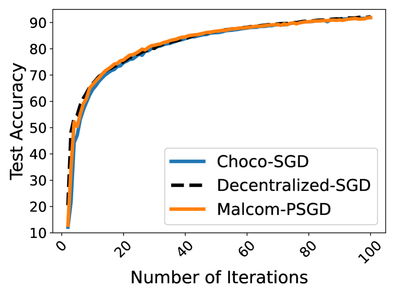
(a) Test accuracy per iterations.

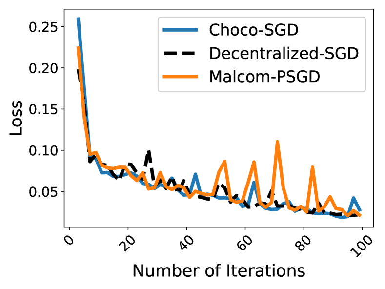
(b) Training loss over iterations.

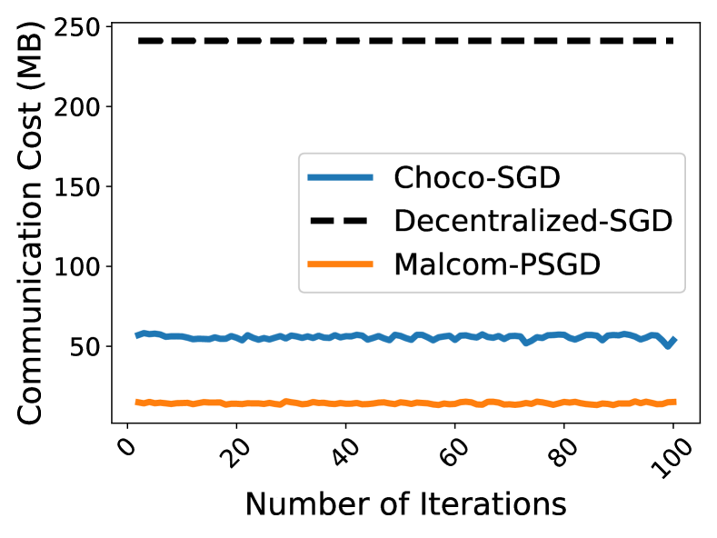
(c) Bits transmitted per iteration.

Figure 1: Synchronous FL with the MNIST dataset and a heterogeneous data distribution

Federated Learning (FL) on MNIST. In this setup we consider 10 nodes within a fully connected DNN. The DNN consists of three fully connected layers with total $d=669,706$ parameters. The training data is distributed in a highly heterogeneous fashion by following Konečný et al. (2016), where each node has data corresponding to exactly two classes/labels with $60$K/$10$K training/testing data in total. The consensus aggregation is performed in a synchronous manner, i.e., at iteration $t$ all the nodes simultaneously perform the aggregation step by (4). Additionally, to validate the efficacy of Malcom-PSGD we use a constant learning rate ($\eta_{t}=.2$) and consensus step size ($\gamma_{t}=1$). Finally, both Malcom-PSGD and Choco-SGD use the quantization scheme in (6) with $3$-bit quantization precision (i.e., $L=8$). In Fig. 1, the results are compared with the error-free decentralized SGD benchmark, which assumes perfect model communication without compression and quantization. It is observed that Choco-SGD and Malcom-PSGD achieve equivalent accuracy and loss as the error-free baseline. However, Malcom-PSGD reduces the communication bit requirements by approximately $74\%$. This matches our analysis of the synchronous setting.

(a) Test accuracy per iterations.

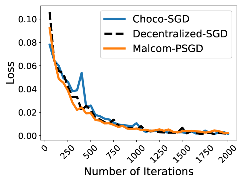
(b) Training loss over iterations.

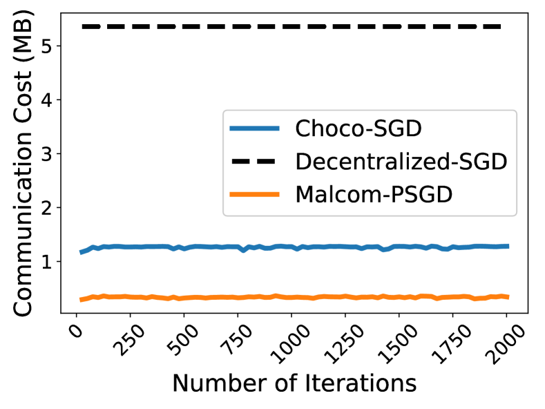
(c) Bits transmitted per iteration.

Figure 2: Asynchronous decentralized learning of MNIST.

Asynchronous Decentralized Learning on MNIST. This setup is identical to the FL setup above, except that we consider pairwise dynamic and asynchronous networking. At each iteration, we randomly pick two nodes for model sharing and aggregation over their communication link, resulting in a time-varying mixing matrix. The results are presented in Fig. 2. Similar to the synchronous case, both Choco-SGD and Malcom-PSGD eventually recover the accuracy and loss of the error-free algorithm, but it should be noted that our algorithm converges at a slightly faster rate. This is because in the asynchronous setting error accumulation during aggregation is more significant due to the high data heterogeneity. Our findings indicate that Malcom-PSGD reduces the communication cost by $94\%$ compared to the error-free baseline and by $74\%$ relative to Choco-SGD. This result highlights the efficiency of Malcom-PSGD in the practical asynchronous setting, which represents numerous real-world situations, including Internet-of-Things (IoT) and device-to-device (D2D) networks.

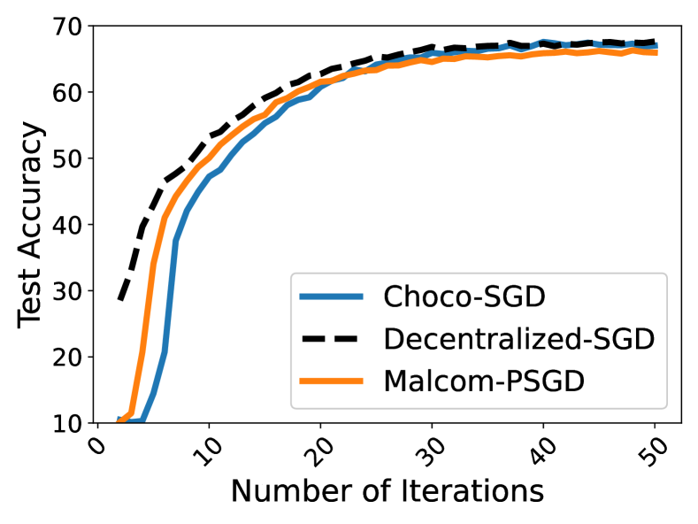
(a) Accuracy per Iterations.

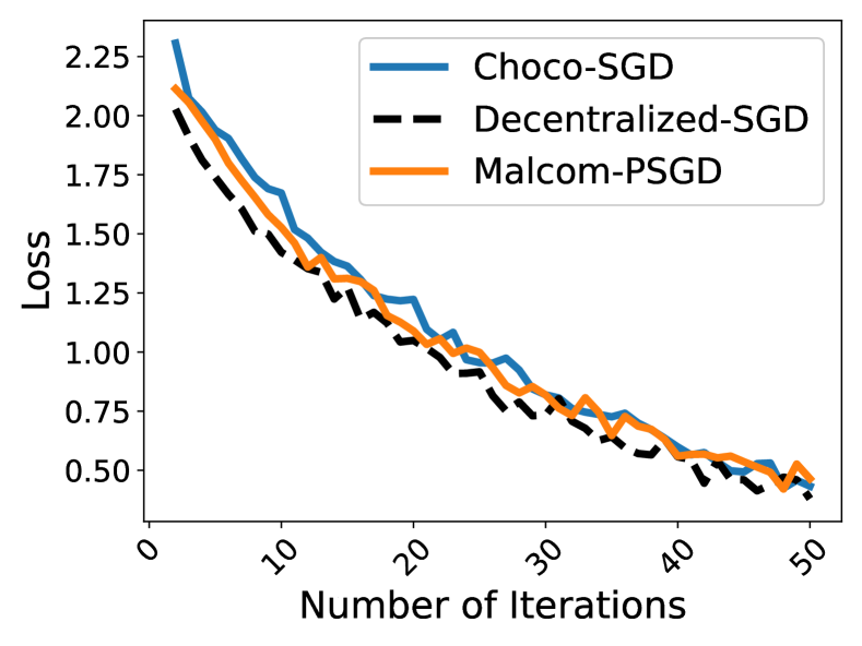
(b) Loss over Iterations.

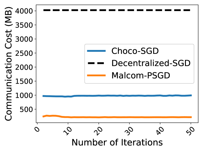
(c) Bits transmitted per iteration.

Figure 3: Synchronous FL with ResNet18 over CIFAR10, where local data is i.i.d. distributed.

FL on CIFAR10. We simulate an FL network with 10 nodes where each node uses the ResNet18 model He et al. (2016) with an i.i.d. distribution of $50,000$ CIFAR10 training samples. Aggregation and communication protocols are the same as those in the above experiments with the MNIST dataset. The results are presented in Fig. 3. We observe similar results to that in Fig. 1, except that Malcom-PSGD converges faster than Choco-SGD. Notably, Malcom-PSGD reduces communication costs from the error-free baseline and Choco-SGD by $95\%$ and $78\%$, respectively.

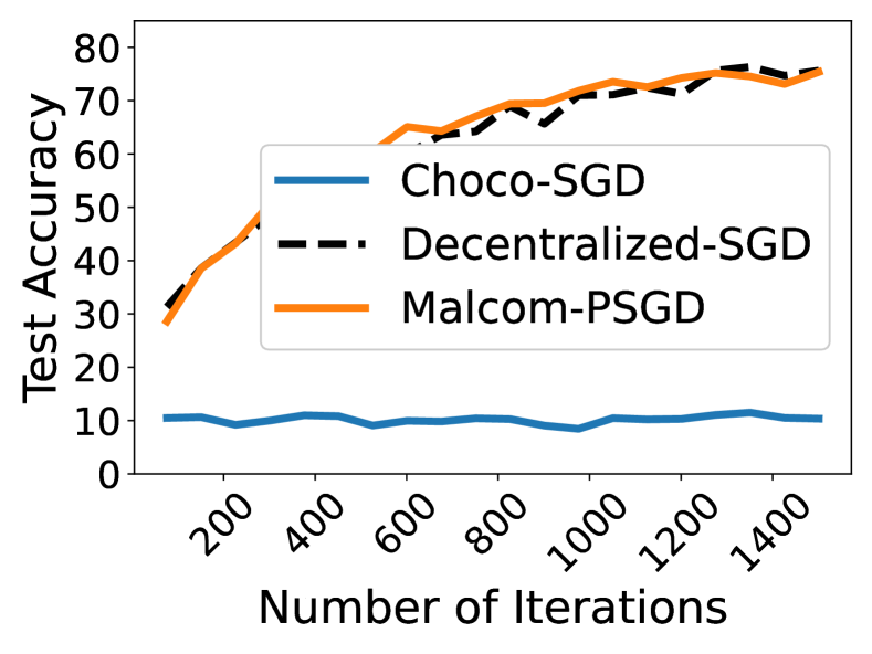
(a) Sync: Acc. versus Iter.

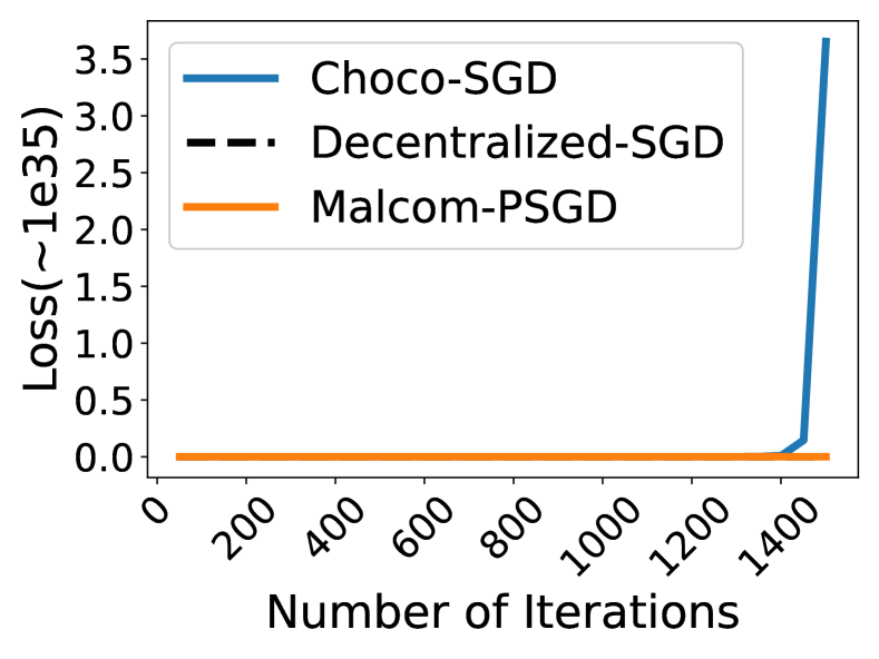
(b) Sync: Loss versus Iter.

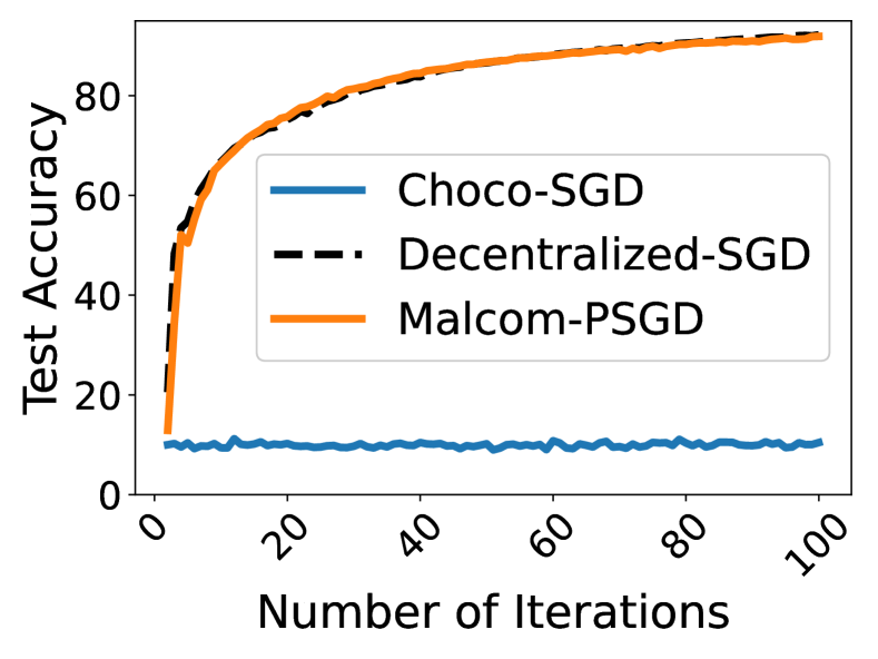
(c) Async: Acc. versus Iter.

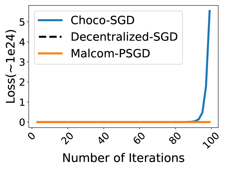
(d) Async: Loss versus Iter.

Figure 4: Decentralzied learning under the communication rate constraints. The loss values of (b) and (d) are on the order of $10^{35}$ and $10^{24}$ respectively.

Learning with Fixed Communication Rates. We simulate decentralized image classification over the MNIST dataset with the aforementioned DNN. Local model residuals are communicated over rate-constrained channels with the channel capacity of $39$ MB/iteration and $1$ MB/iteration for the synchronous and asynchronous systems, respectively. Fig. 4 plots the test accuracy and training loss under the stringent communication rate constraints. While Choco-SGD diverges due to excessive quantization error, Malcom-PSGD capitalizes on more efficient communication and thus allows high-precision quantization.

7 Conclusion

We introduced the Malcom-PSGD algorithm for decentralized learning with finite-sum, smooth, and non-convex loss functions. Our approach sparsifies local models by non-smooth $\ell_{1}$ regularization, rendering the implementation of the conventional SGD-based model updating challenging. To address this challenge, we adopted the decentralized proximal SGD method to minimize the regularized loss, where the residuals of local SGD updates are shared and aggregated prior to the local proximal optimization. Furthermore, we employed dithering-based gradient quantization and vector source coding schemes to compress model communication and leverage the low entropy of the updates to reduce the communication cost. By characterizing data sub-sampling and compression errors as perturbations in the proximal operation, we quantified the impact of gradient compression on training performance and established the convergence rate of Malcom-PSGD with diminishing stepsizes. Moreover, we analyzed the communication cost in terms of the asymptotic code rate for the proposed algorithm. Numerical results validate the theoretical findings and demonstrate the improvement of our method in both learning performance and communication efficiency.

Appendix A Appendix

A.1 Encoding Algorithm

The following algorithm describes the encoding scheme proposed in Woldemariam et al. (2023). In this scheme, the type vector is assumed to be in descending order, while implementation allows for an unordered type vector. In Algorithm 2, the notation $[x]$ denotes the nearest integer of $x$.

A.2 Matrix Representation of Malcom-PSGD and Useful Lemmas

To facilitate our proofs, we recast Malcom-PSGD into an equivalent matrix form. Specifically, we define ${\bm{Y}}^{(t)}=[{\bm{y}}_{1}^{(t)},\cdots,{\bm{y}}_{n}^{(t)}]$, ${\bm{Z}}^{(t)}=[{\bm{z}}_{1}^{(t)},\cdots,{\bm{z}}_{n}^{(t)}]$, ${\bm{Q}}^{(t)}=[{\bm{q}}_{1}^{(t)},\cdots,{\bm{q}}_{n}^{(t)}]$, ${\bf\xi}^{(t)}=[\xi_{1}^{(t)},\cdots,\xi_{n}^{(t)}]^{T}$ , and $\nabla F({\bm{X}}^{(t)},\xi^{(t)})=[\nabla F_{i}({\bm{x}}_{1}^{(t)},\xi_{1}^{(t)}),\cdots,\nabla F_{n}({\bm{x}}_{n}^{(t)},\xi_{n}^{(t)})]$. Together with the matrices ${\bm{X}}^{(t)}$ and $\overline{\bm{X}}^{(t)}$ defined in Section 5, we have the matrix form of Alg. 1, as shown in Alg. 3.

We also provide two useful results for the proof.

Lemma 1.

For any ${\bf A},{\bf B}$ with the same dimension, we have, for any $\alpha>0$:

$$\lVert{{\bf A}+{\bf B}}\rVert_{F}^{2}\leq(1+\alpha)\lVert{{\bf A}}\rVert_{F}^{2}+(1+\alpha^{-1})\lVert{{\bf B}}\rVert_{F}^{2},$$ (17)

$$\|{\bm{A}}{\bm{B}}\|_{F}\leq\|{\bm{A}}\|_{F}\|{\bm{B}}\|_{2}.$$ (18)

Lemma 2.

For the mixing matrix ${\bm{W}}$ satisfying Assumption 1, we have, for any $k>0$,

$$\left\|{\bm{W}}^{k}-\frac{1}{n}{\bf 1}{\bf 1}^{\top}\right\|_{2}\leq\lambda_{2}^{k}=(1-\delta)^{k},$$ (19)

$$\left\|{\bf I}-{\bm{W}}\right\|_{2}^{2}=\lambda_{n}^{2},$$ (20)

where we define $\delta:=1-\lambda_{2}$.

Proof.

See (Koloskova et al., 2019, Lemma 16). ∎

Algorithm 2 The source encoding scheme.

1:function Encode(${\bm{q}}$, $L$)

2:     Compute $\bm{t}({\bm{q}})$ and encode it with Elias omega encoding.

3:     Initialize $\mathcal{I}=\{1,\dots,N\}$.

4:     for $\ell=1,\dots,L-1$ do

5:         $\mathcal{I}^{\prime}=\emptyset$, $\mathcal{R}_{\ell}=\emptyset$.

6:         Compute $M_{\ell}=[(\ln 2)(N-\sum_{m\leq\ell}t_{m}({{\bm{q}}}))/t_{\ell}({{\bm{q}}})]$.

7:         $r=0$.

8:         for $j\in\mathcal{I}$ do

9:              if $\delta(q_{j}-\ell)=0$ then

10:                  $\mathcal{R}_{\ell}=\mathcal{R}_{\ell}\cup\{r\}$.

11:                  if $|\mathcal{R}_{\ell}|<t_{\ell}({{\bm{q}}})$ then

12:                       Encode $r$ by Golomb coding with parameter $M_{\ell}$.                   

13:                  $r=0$.

14:                  $\mathcal{I}^{\prime}=\mathcal{I}^{\prime}\cup\{n\}$.

15:              else

16:                  $r=r+1$.               

17:              $\mathcal{I}=\mathcal{I}$ $\backslash$ $\mathcal{I}^{\prime}$.               

Algorithm 3 The matrix form of Malcom-PSGD.

1:${\bm{X}}^{(0)},{\bm{Y}}^{(-1)}=0$.

2:for $t\in[0,\ldots,T-1]$ do $\triangleright$ All nodes $i$ do in parallel

3:     ${\bm{X}}^{(t+1/2)}={\bm{X}}^{(t)}-\eta_{t}\nabla{\bm{F}}\left({\bm{X}}^{(t)},{\bf\xi}^{(t)}\right)$

4:     $\bm{Q}^{(t)}=Q({\bm{X}}^{(t+1/2)}-{\bm{Y}}^{(t-1)}$) $\triangleright$ Residual quantization; see (6).

5:     for $j\in\mathcal{N}_{i}$ do

6:         Encode and send $\bm{Q}^{(t)}$ $\triangleright$ Residual communication with source encoding.

7:         Receive and decode $\bm{Q}^{(t)}$ $\triangleright$ Receiver decoding.

8:         ${\bm{Y}}^{(t)}=\bm{Q}^{(t)}+{\bm{Y}}^{(t-1)}$      

9:     ${\bm{Z}}^{(t+1)}=(1-\gamma_{t}){\bm{X}}^{(t+1/2)}+\gamma_{t}{\bm{Y}}^{(t)}{\bm{W}}$$\triangleright$ Consensus aggregation; cf. (4).

10:     ${\bm{X}}^{(t+1)}=\mathcal{S}_{\eta_{t}\mu}\left({\bm{Z}}^{(t+1)}\right)$$\triangleright$ Proximal optimization by soft-thresholding; see (7).

A.3 The Quantization Scheme in (6) Satisfies Assumption 2

We denote the effective quantization scheme combining (6) and the de-normalization procedure at the receiver end by $\hat{Q}(\cdot)$. Specifically, for any input vector ${\bm{x}}\in\mathbb{R}^{d}$, the $i$-th entry of the output is given by $\hat{Q}(x_{i})=(\max{({\bm{x}})}-\min{({\bm{x}})})Q(x_{i})+\min{({\bm{x}})}$. Let $h(x_{i})=\dfrac{x_{i}-\min({\bm{x}})}{\max({\bm{x}})-\min({\bm{x}})}$, $r({\bm{x}})=\max({\bm{x}})-\min({\bm{x}})$, and $m=\min({\bm{x}})$. We have

$$\hat{Q}(x_{i})=\dfrac{1}{\tau}\left(\zeta\left(h(x_{i})\right)r({\bm{x}})+m\right).$$

From (Alistarh et al., 2017, Lemma 3.1), the operator $\zeta(\cdot)$ is unbiased, i.e., $\mathbb{E}[\zeta(h({\bm{x}}))]=h({\bm{x}})$, where the expectation is taken w.r.t. the uniform dithering process. Moreover, let $l$ be the quantization region of $x_{i}$ such that $h(x_{i})\in[l/L,(l+1/L)]$. Let $p_{i}$ denote the probability that $h(x_{i})$ is mapped to $(l+1)/L$, where we have $p_{i}=h(x_{i})L-l$. In other words, we have $\zeta(h(x_{i}),L)$ equal to $(l+1)/L$ with probability $p_{i}$ and equal to $(l+1)/L$ with probability $1-p_{i}$. Therefore, we have

$$\mathbb{E}[\zeta(h(x_{i}),L)^{2}] =\mathbb{E}[\zeta(h(x_{i}),L)]^{2}+\mathrm{Var}(\zeta(h(x_{i}),L))=h^{2}(x_{i})+\dfrac{p(1-p)}{L^{2}}\leq h^{2}(x_{i})+\dfrac{1}{4L^{2}},$$

where $\mathrm{Var}(\cdot)$ denotes the variance of the input random variable, and the last inequality follows from $p(1-p)\leq 1/4$.

Note that

$$\mathbb{E}[\|\hat{Q}({\bm{x}})\|^{2}] =\frac{1}{\tau^{2}}\mathbb{E}\left[\sum^{d}_{i=1}\left(r({\bm{x}})\zeta(h(x_{i}),L)+m\right)^{2}\right]$$

$$=\frac{1}{\tau^{2}}\left(\sum^{d}_{i=1}\mathbb{E}\left[r^{2}({\bm{x}})\zeta(h(x_{i}),L)^{2}\right]+\sum^{d}_{i=1}\mathbb{E}\left[2r({\bm{x}})m\zeta(h(x_{i}),L)\right]+\sum^{d}_{i=1}m^{2}\right)$$

$$\leq\frac{1}{\tau^{2}}\left(r^{2}({\bm{x}})\sum^{d}_{i=1}\left(h^{2}(x_{i})+\dfrac{1}{4L^{2}}\right)+2r({\bm{x}})m\sum^{d}_{i=1}h(x_{i})+dm^{2}\right).$$ (21)

For $h(\cdot)$, we have

$$\sum^{d}_{i=1}h(x_{i}) =\dfrac{1}{r({\bm{x}})}(-dm+\sum^{d}_{i=1}x_{i}),$$ (22)

$$\sum^{d}_{i=1}h^{2}(x_{i}) =\dfrac{1}{r^{2}({\bm{x}})}\sum^{d}_{i=1}x_{i}^{2}-\dfrac{2m}{r^{2}({\bm{x}})}\sum^{d}_{i=1}x_{i}+\dfrac{dm^{2}}{r^{2}({\bm{x}})}.$$ (23)

Substituting (22) and (23) into (21) we have:

$$\mathbb{E}[\|\hat{Q}({\bm{x}})\|^{2}] =\frac{1}{\tau^{2}}\left(\|{\bm{x}}\|_{2}^{2}+r^{2}({\bm{x}})\dfrac{d}{4L^{2}}\right)\overset{(a)}{\leq}\frac{1}{\tau^{2}}\left(1+\dfrac{d}{L^{2}}\right)\|{\bm{x}}\|_{2}^{2}\overset{(a)}{=}\frac{\left\lVert{\bm{x}}\right\rVert_{2}^{2}}{\tau},$$

where $(a)$ follows from $r^{2}({\bm{x}})\leq 4\|{\bm{x}}\|_{\infty}^{2}\leq 4\|{\bm{x}}\|_{2}^{2}$ and $(b)$ follows from the definition of $\tau$. Finally, we have

$$\mathbb{E}\left[\|\hat{Q}({\bm{x}})-{\bm{x}}\|^{2}\right] =\mathbb{E}\left[\sum^{d}_{i=1}\hat{Q}(x_{i})^{2}\right]-2\mathbb{E}\left[\sum^{d}_{i=1}\hat{Q}(x_{i})x_{i}\right]+\mathbb{E}\left[\sum^{d}_{i=1}x_{i}^{2}\right]$$

$$\leq\dfrac{1}{\tau}\|{\bm{x}}\|^{2}-\dfrac{2}{\tau}\|{\bm{x}}\|^{2}+\|{\bm{x}}\|^{2}=\left(1-\dfrac{1}{\tau}\right)\|{\bm{x}}\|^{2},$$

which completes the proof.

A.4 Proof of Theorem 1

Before proving Theorem 1, we state the following two lemmas.

Lemma 3.

Suppose $\gamma_{t}\leq\frac{1-\lambda_{2}}{4\tau}$, then for any $\theta>0$ we have:

$$\mathbb{E}_{Q_{t+1}}\left[\left(1+\theta^{-1}\right)\left\|{\bm{Z}}^{(t+1)}-\overline{\bm{Z}}^{(t+1)}\right\|_{F}^{2}+\left\|{\bm{X}}^{(t+3/2)}-{\bm{Y}}^{(t+1)}\right\|_{F}^{2}\right]$$

$$\leq(1+\theta^{-1})(1-\omega)\left(\left\|{\bm{X}}^{(t+1/2)}-\overline{\bm{X}}^{(t+1/2)}\right\|_{F}^{2}+\left\|{\bm{X}}^{(t+1/2)}-{\bm{Y}}^{(t)}\right\|_{F}^{2}\right)$$ (24)

$$~{}~{}~{}~{}+(1+\theta)\eta_{t}^{2}\left\lVert\nabla{\bm{F}}\left({\bm{X}}^{(t+1)},\xi^{(t+1)}+\bm{\Phi}^{(t+1)}\right)\right\rVert_{F}^{2},$$ (25)

where $\omega=\frac{(1-\lambda_{2})^{2}}{8\tau}\leq\frac{1}{8}$.

Proof.

See Appendix A.7.1. ∎

Lemma 3 provides a useful bound on the aggregation error in terms of the model averaging error and the quantization error.

Lemma 4.

Consider a sequence $\{r_{t}\}_{t\geq 1}$ s.t.

$$r_{t+1}\leq(1-c/2)r_{t}+\frac{2}{c}\eta_{t}^{2}A,$$ (26)

for positive constants $c$ and $A$; and $\eta_{t}=\frac{b}{(t+a)^{\epsilon}}$ with $a,b>0$ and $\epsilon\in(0,1]$.

Moreover, suppose $\epsilon<\frac{c}{4(2-c)}a$ and $r_{0}\leq\frac{A\eta_{0}^{2}}{c}\frac{4(a+2\epsilon)}{ac+4(c-2)\epsilon}$. We have

$$r_{t}\leq\frac{\eta_{t}^{2}A}{c}\frac{4(a+2\epsilon)}{ac+4(c-2)\epsilon},\forall t.$$ (27)

Proof.

See Appendix A.7.2. ∎

Equipped with the above results, we are ready to prove Theorem 1. Define the following auxiliary functions:

$$\mathcal{L}_{\eta_{t},\gamma_{t}}({\bm{X}})=\sum_{i=1}^{n}\left(F_{i}({\bm{x}}_{i})+\frac{\gamma_{t}}{2\eta_{t}}\left\|{\bm{x}}_{i}\right\|_{{\bf I}-{\bm{W}}}^{2}\right)={\bf 1}^{T}{\bm{F}}({\bm{X}})+\frac{\gamma_{t}}{2\eta_{t}}\left\|{\bm{X}}\right\|_{{\bf I}-{\bm{W}}}^{2},$$ (28)

$$\mathcal{M}_{\eta_{t},\gamma_{t}}({\bm{X}})=\mathcal{L}_{\eta_{t},\gamma_{t}}({\bm{X}})+\mu\left\|{\bm{X}}\right\|_{1,1}.$$ (29)

Then, Step 9 of Alg. 3 can be represented as

$${\bm{X}}^{(t+1)}=\text{prox}\left((1-\gamma_{t}){\bm{X}}^{(t)}+\gamma_{t}{\bm{Y}}^{(t)}{\bm{W}}-\eta_{t}\nabla{\bm{F}}({\bm{X}}^{(t)},\xi^{(t)})\right)$$

$$={\bm{X}}^{(t)}-\eta_{t}\left(\underbrace{\nabla{\bm{F}}({\bm{X}}^{(t)},\xi^{(t)})+\frac{\gamma_{t}}{\eta_{t}}{\bm{X}}^{(t)}({\bf I}-{\bm{W}})}_{\nabla\mathcal{L}_{\eta_{t},\gamma_{t}}({\bm{X}}^{(t)};\xi_{t})}+\Phi^{(t+1)}\right)-\gamma_{t}\left(\underbrace{{\bm{X}}^{(t)}-{\bm{Y}}^{(t-1)}-Q({\bm{X}}^{(t)}-{\bm{Y}}^{(t-1)})}_{\text{Quantization error }\triangleq{\bm{E}}_{t}}\right){\bm{W}},$$ (30)

for some subdifferential $\Phi^{(t+1)}\in\partial\left(\mu\left\|{\bm{X}}^{(t+1)}\right\|_{1,1}\right)$. We observe the following properties:

Observation 1.

Every subgradient of the regularization function $\bm{\phi}\in\partial(\mu\left\lVert{\bm{x}}\right\rVert_{1})$ has a bounded norm as $\left\lVert\bm{\phi}\right\rVert_{2}\leq\mu\sqrt{d}$. Under Assumption 3, we have $\mathbb{E}[\left\lVert\nabla F({\bm{X}};{\bf\xi})+\bm{\Phi}\right\rVert_{F}^{2}]\leq 2n(2G^{2}+2\sigma^{2}+\mu^{2}d)$ for any $\bm{\phi}_{i}\in\partial(\mu\left\lVert{\bm{x}}_{i}\right\rVert_{1})$, ${\bm{X}}$, and $\bf\xi$.

Define a sequence $\{r_{t}\}_{t}$ such that

$$r_{t}=\mathbb{E}\left[\left\|{\bm{X}}^{(t)}-\overline{\bm{X}}^{(t)}\right\|_{F}^{2}+\left\|{\bm{X}}^{(t+1/2)}-{\bm{Y}}^{(t)}\right\|_{F}^{2}\right].$$ (31)

At iteration $t+1$, we have

$$r_{t+1}=\mathbb{E}\left[\left\lVert{\bm{Z}}^{(t+1)}-\overline{\bm{Z}}^{(t+1)}+\eta_{t+1}\left(\Phi^{(t+1)}\right)\left(\frac{{\bf 1}{\bf 1}^{T}}{n}-{\bf I}\right)\right\rVert_{F}^{2}\right]+\mathbb{E}\left[\left\lVert{\bm{X}}^{(t+3/2)}-{\bm{Y}}^{(t+1)}\right\rVert_{F}^{2}\right]$$

$$\leq\mathbb{E}\left[(1+{\alpha}^{-1})\left\lVert{\bm{Z}}^{(t+1)}-\overline{\bm{Z}}^{(t+1)}\right\rVert_{F}^{2}+\left\lVert\nabla{\bm{X}}^{(t+1)}-{\bm{Y}}^{(t+1)}\right\rVert_{F}^{2}\right]+(1+{\alpha})\eta_{t}^{2}\mathbb{E}\left[\left\lVert\Phi^{(t+1)}\right\rVert_{F}^{2}\right]\left(\left\lVert\frac{{\bf 1}{\bf 1}^{T}}{n}-{\bf I}\right\rVert_{2}^{2}\right)$$

$$\overset{(\ref{eq:lem2_eq}),\theta={\alpha}}{\leq}(1+{\alpha}^{-1})(1-\omega)\left\lVert{\bm{X}}^{(t+1/2)}-\overline{\bm{X}}^{(t+1/2)}\right\rVert^{2}_{F}+(1-\omega)\left\lVert{\bm{X}}^{(t+1/2)}-Y^{(t)}\right\rVert^{2}_{F}$$

$$~{}~{}~{}~{}+(1+\alpha)(\eta_{t}^{2})2n\mu^{2}d+(1+\alpha)\eta_{t}^{2}\left\lVert\nabla F\left({\bm{X}}^{(t+1)},\xi^{(t+1)}\right)+\Phi^{(t+1)}\right\rVert_{F}^{2}$$

$$\leq(1+{\alpha}^{-1})(1+\beta^{-1})(1-\omega)\left\lVert{\bm{X}}^{(t)}-\overline{\bm{X}}^{(t)}\right\rVert^{2}_{F}+(1+\beta)(1-\omega)\eta_{t}^{2}\left\lVert{\bm{F}}({\bm{X}}^{(t+1)})\right\rVert_{F}^{2}$$

$$~{}~{}~{}~{}+(1+\alpha)(\eta_{t}^{2})2n\mu^{2}d+(1-\omega)\left\lVert{\bm{X}}^{(t+1/2)}-Y^{(t)}\right\rVert_{F}^{2}+(1+\alpha)\eta_{t}^{2}\left\lVert\nabla{\bm{F}}\left({\bm{X}}^{(t+1)},\xi^{(t+1)}\right)+\Phi^{(t+1)}\right\rVert_{F}^{2}$$

$$\overset{{\beta=6/(\omega(1-\omega)})}{\leq}(1+{\alpha}^{-1})(1+\dfrac{\omega(1-\omega)}{6})(1-\omega)r_{t}+(1+{\alpha})(1+\dfrac{6}{\omega(1-\omega)})(1-\omega)4n\eta_{t}^{2}(2G^{2}+2\sigma^{2}+\mu^{2}d)$$

$$\overset{\alpha=\omega/{(3-\omega)}}{\leq}(1+\omega/2)(1-\omega)r_{t}+\left(\dfrac{9}{\omega}\right)4n\eta_{t}^{2}(2G^{2}+2\sigma^{2}+\mu^{2}d)$$

$$\leq(1-\omega/2)r_{t}+\frac{36}{\omega}n\eta_{t}^{2}(2G^{2}+2\sigma^{2}+\mu^{2}d).$$

Combining the recursion of $r_{t+1}$ and Lemma 4, we have (26) with $A=18n(2G^{2}+2\sigma^{2}+\mu^{2}d)$. Applying Lemma 4 and assuming $\epsilon<\frac{\omega}{4(2-\omega)}a$, we have

$$r_{t}\leq\frac{56(a+2\epsilon)}{\omega(a\omega+4(\omega-2)\epsilon)}n\eta_{t}^{2}(2G^{2}+2\sigma^{2}+\mu^{2}d).$$ (32)

To prove (14), we first note that if $a\geq 8\epsilon/\omega$,

$$\frac{a}{\epsilon}\geq\frac{8}{\omega}>\frac{4(2-\omega)}{\omega}.$$

(32) follows from the assumption of $\left\|{\bm{x}}^{(0)}\right\|=0$. Furthermore, define the function $h(x)=\frac{1+2x}{\omega+4(\omega-2)x}$. We have

$$h^{\prime}(x)=2\cdot\frac{\omega+4(\omega-2)x-2(1+2x)(\omega-2)}{(\omega+4(\omega-2)x)^{2}}=\frac{8-2\omega}{(\omega+4(\omega-2)x)^{2}}>0.$$

For $\epsilon/a\leq\omega/8$, we have

$$h(\epsilon/a)\leq h(\omega/8)=\frac{2+\omega/2}{\omega^{2}}\leq\frac{33}{16\omega^{2}},$$ (33)

where the last inequality follows from $\omega\leq 1/8$. Substituting (33) into (32) and applying $\mathbb{E}[\left\|{\bm{X}}^{t}-\overline{\bm{X}}^{t}\right\|_{F}^{2}]\leq r_{t}$, we have

$$\mathbb{E}\left\|{\bm{X}}^{(t)}-\overline{\bm{X}}^{(t)}\right\|_{F}^{2}\leq r_{t}\leq\frac{56}{\omega}n\eta_{t}^{2}(2G^{2}+2\sigma^{2}+\mu^{2}d)h(\omega/8)\leq\frac{C}{\omega^{3}}n\eta_{t}^{2}(2G^{2}+2\sigma^{2}+\mu^{2}d),$$ (34)

where $C<116$ is a constant.

A.5 Corollary 1

Theorem 1 implies the following corollary that will be useful in the convergence proof.

Corollary 1.

Under the same conditions of Theorem 1, one has that

$$\mathbb{E}\left\lVert\overline{\bm{x}}^{(t+1)}-\overline{\bm{x}}^{(t)}\right\rVert^{2}\leq\frac{1}{n}\sum_{i=1}^{n}\mathbb{E}\left\lVert{\bm{x}}_{i}^{(t+1)}-{\bm{x}}_{i}^{(t)}\right\rVert^{2}\leq(2G^{2}+2\sigma^{2}+\mu^{2}d)\left(1+6\sqrt{\frac{C}{32\omega^{3}}+1}\right)^{2}\eta^{2}_{t},$$ (35)

where $C<116$ is the constant defined in Theorem 1.

Proof.

Note that

$$\left\lVert\overline{\bm{X}}^{(t+1)}-\overline{\bm{X}}^{(t)}\right\rVert_{F}^{2}=\left\lVert({\bm{X}}^{(t+1)}-{\bm{X}}^{(t)}){\bf 1}{\bf 1}^{T}/n\right\rVert_{F}^{2}\leq\left\lVert{\bm{X}}^{(t+1)}-{\bm{X}}^{(t)}\right\rVert_{F}^{2}.$$ (36)

Applying (17), for any ${\alpha},\beta>0$,

$$\mathbb{E}\left\lVert{\bm{X}}^{(t+1)}-{\bm{X}}^{(t)}\right\rVert^{2}_{F}\leq(1+{\alpha}^{-1})\mathbb{E}\left\lVert{\bm{X}}^{(t+1)}-\overline{\bm{X}}^{(t+1)}\right\rVert^{2}_{F}$$

$$+(1+{\alpha})(1+\beta^{-1})\mathbb{E}\left\lVert{\bm{X}}^{(t)}-\overline{\bm{X}}^{(t)}\right\rVert^{2}_{F}+(1+{\alpha})(1+\beta)\mathbb{E}\left\lVert\overline{\bm{X}}^{(t+1)}-\overline{\bm{X}}^{(t)}\right\rVert^{2}_{F}.$$ (37)

The last term in (A.5) can be simplified as

$$\mathbb{E}\left\lVert\overline{\bm{X}}^{(t+1)}-\overline{\bm{X}}^{(t)}\right\rVert_{F}^{2} \leq\mathbb{E}\left\lVert\eta_{t}\left(\nabla{\bm{F}}({\bm{X}}^{(t)},\xi^{(t)})+\Phi^{(t+1)}\right)-\gamma_{t}({\bm{X}}^{(t)}-{\bm{Y}}^{(t)})\right\rVert^{2}_{F}\left\lVert{\bf 1}{\bf 1}^{T}/n\right\rVert^{2}_{2}$$

$$\leq 2\eta^{2}_{t}\mathbb{E}\left\lVert\nabla{\bm{F}}({\bm{X}}^{(t)},\xi^{(t)})+\Phi^{(t+1)}\right\rVert_{F}^{2}+2\gamma_{t}^{2}\mathbb{E}\left\lVert{\bm{X}}^{(t)}-{\bm{Y}}^{(t)}\right\rVert_{F}^{2}$$

$$\leq 4n(2G^{2}+2\sigma^{2}+\mu^{2}d)\eta^{2}_{t}+2\gamma_{t}^{2}\mathbb{E}\left\lVert{\bm{X}}^{(t)}-{\bm{Y}}^{(t)}\right\rVert_{F}^{2}.$$ (38)

Combining (A.5), (A.5), and (31), for $\forall{\alpha},\beta>0$,

$$\mathbb{E}[\left\lVert{\bm{X}}^{(t+1)}-{\bm{X}}^{(t)}\right\rVert^{2}_{F}]\leq (1+{\alpha}^{-1})r_{t+1}+(1+{\alpha})r_{t}\max\{1+\beta^{-1},2\gamma_{t}^{2}(1+\beta)\}$$

$$+(1+{\alpha})(1+\beta)4n(2G^{2}+2\sigma^{2}+\mu^{2}d)\eta^{2}_{t}.$$ (39)

In particular, setting $\beta=8$, we have $1+\beta^{-1}=9/8$ and $2\gamma_{t}^{2}(1+\beta)=18/\gamma_{t}^{2}\leq 9/8$. Applying (34),

$$\mathbb{E}[\left\lVert{\bm{X}}^{(t+1)}-{\bm{X}}^{(t)}\right\rVert^{2}_{F}]\leq \left(1+{\alpha}^{-1}+(1+{\alpha})\left(\frac{9C}{8\omega^{3}}+36\right)\right)n(2G^{2}+2\sigma^{2}+\mu^{2}d)\eta^{2}_{t}.$$ (40)

By the inequality of arithmetic and geometric means, we have

$$1+{\alpha}^{-1}+(1+{\alpha})\left(\frac{9C}{8\omega^{3}}+36\right)\geq\left(1+\sqrt{\frac{9C}{8\omega^{3}}+36}\right)^{2},$$ (41)

where the inequality holds if ${\alpha}^{-2}=\frac{9C}{8\omega^{3}}+36$. Combining (40) and (41) completes the proof. ∎

A.6 Proof of Theorem 2

We first state the following proposition which provides a bound for the average residual:

Proposition 1 (Average residual).

Suppose we initialize the model by ${\bm{x}}^{(0)}={\bm{y}}^{(-1)}=\bf 0$. The residual to be transmitted at iteration $0$ is $\bf 0$. Under the conditions of Theorem 1, the average residual to be quantized and transmitted (i.e., the quantity applied to $Q(\cdot)$) in iteration $t+1,t=0,1,\cdots,$ is bounded by

$$\frac{1}{n}\sum_{i=1}^{n}\mathbb{E}[\left\lVert{\bm{x}}_{i}^{(t+1)}-{\bm{y}}_{i}^{(t)}\right\rVert^{2}]\leq 2\left(1+\sqrt{\frac{C}{\omega}}\frac{1-\gamma_{t}\lambda_{n}}{\omega}\right)^{2}(2G^{2}+2\sigma^{2}+\mu^{2}d)\eta_{t}^{2},$$ (42)

where $C<116$ is the constant defined in Theorem 1.

Proof.

See Appendix A.7.3. ∎

We prove the convergence of Malcom-PSGD by using Proposition 1 and Theorem 1 as follows. First, note that $\eta_{t}\leq\frac{1}{a^{\epsilon}}\leq\frac{1-(1-\lambda_{n})\gamma_{t}}{L},\forall t$ with $\gamma_{t}\leq\frac{1-a^{-\epsilon}}{1-\lambda_{n}}$. Leveraging $L^{\prime}=L+\gamma_{t}\eta_{t}^{-1}(1-\lambda_{n})$ in Observation LABEL:obs2, we have $L^{\prime}\leq\eta_{t}^{-1}$. Following (Zeng & Yin, 2018a, Eqs. (88)-(89) ), for any given ${\bm{U}}\in\mathbb{R}^{d\times n}$ that is independent to $t$,

$$\mathcal{M}_{\eta_{t},\gamma_{t}}({\bm{U}})-\mathcal{M}_{\eta_{t},\gamma_{t}}({\bm{X}}^{(t+1)})\geq\left<\nabla\mathcal{L}_{\eta_{t},\gamma_{t}}({\bm{X}}^{(t)})+\bm{\Phi}^{(t+1)},{\bm{U}}-{\bm{X}}^{(t+1)}\right>-\frac{L^{\prime}}{2}\left\|{\bm{X}}^{(t+1)}-{\bm{X}}^{(t)}\right\|_{F}^{2},$$

where $\bm{\Phi}^{(t+1)}\in\partial(\mu\left\lVert{\bm{X}}^{(t+1)}\right\rVert_{1,1})$. Substituting $\Phi^{(t+1)}$ in (30) and taking ${\bm{U}}$ to be an optimal solution ${\bm{X}}^{\star}\in\mathcal{X}^{\star}$,

$$\mathbb{E}[\mathcal{M}_{\eta_{t},\gamma_{t}}({\bm{X}}^{(t+1)})-\mathcal{M}_{\eta_{t},\gamma_{t}}({\bm{X}}^{\star})]$$

$$\leq-\eta_{t}^{-1}\mathbb{E}\left<{\bm{X}}^{(t)}-{\bm{X}}^{(t+1)}-\gamma_{t}({\bm{X}}^{(t)}-{\bm{Y}}^{(t)}){\bm{W}},{\bm{X}}^{\star}-{\bm{X}}^{(t+1)}\right>+\frac{L^{\prime}}{2}\mathbb{E}\left\lVert{\bm{X}}^{(t+1)}-{\bm{X}}^{(t)}\right\rVert_{F}^{2}$$

$$~{}~{}~{}~{}-\underbrace{\left<\mathbb{E}_{t}[\nabla\mathcal{L}_{\eta_{t},\gamma_{t}}({\bm{X}}^{(t)})-\nabla\mathcal{L}_{\eta_{t},\gamma_{t}}({\bm{X}}^{(t)};\xi^{t})],{\bm{X}}^{\star}-\mathbb{E}_{t+1}[{\bm{X}}^{(t+1)}]\right>}_{=0}$$

$$\overset{L^{\prime}\leq\eta_{t}^{-1}}{\leq}\frac{\eta_{t}^{-1}}{2}\mathbb{E}\left\lVert{\bm{X}}^{(t+1)}-{\bm{X}}^{(t)}\right\rVert_{F}^{2}-\eta_{t}^{-1}\mathbb{E}\left<{\bm{X}}^{(t)}-{\bm{X}}^{(t+1)}-\gamma_{t}({\bm{X}}^{(t)}-{\bm{Y}}^{(t)}){\bm{W}},{\bm{X}}^{\star}-{\bm{X}}^{(t+1)}\right>$$

$$=\frac{1}{2\eta_{t}}(\mathbb{E}\left\lVert{\bm{X}}^{(t)}-{\bm{X}}^{\star}\right\rVert_{F}^{2}-\mathbb{E}\left\lVert{\bm{X}}^{(t+1)}-{\bm{X}}^{\star}\right\rVert_{F}^{2})+\gamma_{t}\eta_{t}^{-1}\mathbb{E}\left<({\bm{X}}^{(t)}-{\bm{Y}}^{(t)}){\bm{W}},{\bm{X}}^{\star}-{\bm{X}}^{(t+1)}\right>$$

$$\leq\frac{1}{2\eta_{t}}\left(\mathbb{E}\left\lVert{\bm{X}}^{(t)}-{\bm{X}}^{\star}\right\rVert_{F}^{2}-\mathbb{E}\left\lVert{\bm{X}}^{(t+1)}-{\bm{X}}^{\star}\right\rVert_{F}^{2}+2\gamma_{t}\mathbb{E}_{t}\left\lVert{\bm{X}}^{(t)}-{\bm{Y}}^{(t)}\right\rVert_{F}\mathbb{E}_{t+1}\left\lVert{\bm{X}}^{\star}-{\bm{X}}^{(t+1)}\right\rVert_{F}\right)$$

$$\overset{\text{Pro. }\ref{prop:avg_residual}}{\leq}\frac{1}{2\eta_{t}}\left(\mathbb{E}\left\lVert{\bm{X}}^{(t)}-{\bm{X}}^{\star}\right\rVert_{F}^{2}-\mathbb{E}\left\lVert{\bm{X}}^{(t+1)}-{\bm{X}}^{\star}\right\rVert_{F}^{2}+2C_{0}\underbrace{\gamma_{t}\eta_{t}\mathbb{E}_{t+1}\left\lVert{\bm{X}}^{\star}-{\bm{X}}^{(t+1)}\right\rVert_{F}}_{\triangleq A_{t+1}}\right),$$ (43)

where $C_{0}$ is a constant given by the square root of the r.h.s. of Theorem 1.

Taking the summation of (43) recursively w.r.t. $k=0,1,...,t$ and using ${\bm{X}}^{(0)}=\bf 0$, we have

$$\sum_{k=0}^{t}\eta_{k}(\mathbb{E}[\mathcal{M}_{\eta_{k},\gamma_{k}}({\bm{X}}^{(k+1)})]-\mathcal{F}^{\star}))\leq\frac{1}{2}\left\lVert{\bm{X}}^{\star}\right\rVert_{F}^{2}+C_{0}\sum_{k=0}^{t}A_{k+1}.$$ (44)

On the other hand, note that

$$\left\lVert{\bm{X}}^{(k+1)}\right\rVert_{1,1} \geq\left\lVert\overline{\bm{X}}^{(k+1)}\right\rVert_{1,1}-\left\lVert{\bm{X}}^{(k+1)}-\overline{\bm{X}}^{(k+1)}\right\rVert_{1,1}\geq\left\lVert\overline{\bm{X}}^{(k+1)}\right\rVert_{1,1}-\sqrt{d}\left\lVert{\bm{X}}^{(k+1)}-\overline{\bm{X}}^{(k+1)}\right\rVert_{F};$$ (45)

and

$$\mathcal{L}_{\eta_{k},\gamma_{k}}({\bm{X}}^{(k+1)}) \geq\mathcal{L}_{\eta_{k},\gamma_{k}}(\overline{\bm{X}}^{(k+1)})+<\nabla\mathcal{L}_{\eta_{k},\gamma_{k}}({\bm{X}}^{(k+1)}),{\bm{X}}^{(k+1)}-\overline{\bm{X}}^{(k+1)}>-\frac{L^{\prime}}{2}\left\lVert{\bm{X}}^{(k+1)}-\overline{\bm{X}}^{(k+1)}\right\rVert_{F}^{2}$$

$$\geq\mathcal{L}_{\eta_{k},\gamma_{k}}(\overline{\bm{X}}^{(k+1)})-G\left\lVert{\bm{X}}^{(k+1)}-\overline{\bm{X}}^{(k+1)}\right\rVert_{F}-\frac{L^{\prime}}{2}\left\lVert{\bm{X}}^{(k+1)}-\overline{\bm{X}}^{(k+1)}\right\rVert_{F}^{2}.$$ (46)

Combining (45) and (A.6) and noting that $\overline{\bm{X}}$ is consensus by definition, we have

$$\mathcal{M}_{\eta_{k},\gamma_{k}}({\bm{X}}^{(k+1)})\geq\mathcal{F}(\overline{\bm{X}}^{(k+1)})-(G+\mu\sqrt{d})\left\lVert{\bm{X}}^{(k+1)}-\overline{\bm{X}}^{(k+1)}\right\rVert_{F}-\frac{L^{\prime}}{2}\left\lVert{\bm{X}}^{(k+1)}-\overline{\bm{X}}^{(k+1)}\right\rVert_{F}^{2}.$$ (47)

Combining (44) and (47) and applying $L^{\prime}\leq\eta_{t}^{-1}$,

$$\sum_{k}\eta_{k}(\mathbb{E}\mathcal{F}(\overline{\bm{X}}^{(k+1)})- \mathcal{F}^{\star})\leq\frac{1}{2}\left\lVert{\bm{X}}^{\star}\right\rVert_{F}^{2}+(G+\mu\sqrt{d})\sum_{k}\eta_{k}\mathbb{E}\left\lVert{\bm{X}}^{(k+1)}-\overline{\bm{X}}^{(k+1)}\right\rVert_{F}$$

$$~{}~{}~{}~{}+\frac{1}{2}\sum_{k}\mathbb{E}\left\lVert{\bm{X}}^{(k+1)}-\overline{\bm{X}}^{(k+1)}\right\rVert_{F}^{2}+C_{0}\sum_{k=0}^{t}A_{k+1}.$$ (48)

Applying Theorem 1 and Corollary 1, we have $\mathbb{E}\left\lVert{\bm{X}}^{(k+1)}-\overline{\bm{X}}^{(k+1)}\right\rVert_{F}=\mathcal{O}(\eta_{k})$ and $\mathbb{E}\left\lVert{\bm{X}}^{(k+1)}-\overline{\bm{X}}^{(k+1)}\right\rVert_{F}^{2}=\mathcal{O}(\eta_{k}^{2})$. Note that the left-hand side of (A.6) equals to $(\sum_{k}\eta_{k})(\mathcal{\overline{F}}_{t}-\mathcal{F}^{\star})$. Therefore,

$$\mathbb{E}\mathcal{\overline{F}}_{t}-\mathcal{F}^{\star}\leq\frac{\frac{1}{2}\left\lVert{\bm{X}}^{\star}\right\rVert_{F}^{2}+C_{3}\sum_{k=0}^{t}\eta_{k}^{2}+C_{0}\sum_{k=0}^{t}{\gamma_{k}\eta_{k}\mathbb{E}\left\lVert{\bm{X}}^{\star}-{\bm{X}}^{(k+1)}\right\rVert_{F}}}{\sum_{k=0}^{t}\eta_{k}},$$ (49)

where the constants $C_{0}$ and $C_{3}$ are given by

$$C_{3}\leq \dfrac{C}{2\omega^{3}}\left(2G^{2}+2\sigma^{2}+\mu^{2}d\right)n,$$

$$C_{0}\leq \sqrt{\dfrac{C}{2\omega^{3}}\left(2G^{2}+2\sigma^{2}+\mu^{2}d\right)n}.$$

Note that $\gamma_{k}\eta_{k}\mathbb{E}\left\lVert{\bm{X}}^{\star}-{\bm{X}}^{(k+1)}\right\rVert_{F}\leq(\left\lVert{\bm{X}}^{\star}\right\rVert_{F}+\mathbb{E}\left\lVert{\bm{X}}^{(k+1)}\right\rVert_{F})\gamma_{k}\eta_{k}\leq(B+\left\lVert{\bm{X}}^{\star}\right\rVert_{F})\gamma_{k}\eta_{k}\leq C_{4}\eta_{k}^{2}$ with $C_{4}\leq B+\|{\bm{X}}^{*}\|_{F}$ and B defined in Assumption 4. From (49), we have

$$\mathbb{E}\mathcal{\overline{F}}_{t}-\mathcal{F}^{\star}\leq\frac{1}{\sum_{k=0}^{t}\eta_{t}}\left(C_{1}+C_{2}\sum_{k=0}^{t}\eta_{t}^{2}\right),$$ (50)

where $C_{1}=\left\lVert{\bm{X}}^{\star}\right\rVert_{F}^{2}/2$ and

$$C_{2}=C_{3}+C_{0}C_{4}\leq \dfrac{C}{2\omega^{3}}\left(2G^{2}+2\sigma^{2}+\mu^{2}d\right)n+\left(B+\|{\bm{X}}^{*}\|_{F}\right)\sqrt{\dfrac{C}{2\omega^{3}}\left(2G^{2}+2\sigma^{2}+\mu^{2}d\right)n}.$$

Finally, applying the result in (Chen, 2012, Sect. 3.2.4) to characterize the order of $\mathcal{O}\left(\dfrac{1}{\sum_{k=1}^{\infty}\eta_{k}}+\dfrac{\sum_{k=1}^{\infty}\eta_{k}^{2}}{\sum_{k=1}^{\infty}\eta_{k}}\right)$, it follows that the right-hand side of (50) exhibits the order of

$$\begin{cases}O(\frac{1}{t^{\epsilon}})&\text{ if }\epsilon\in(0,\frac{1}{2}),\\ O(\frac{\ln t}{\sqrt{t}})&\text{ if }\epsilon=\frac{1}{2},\\ O(\frac{1}{t^{(1-\epsilon)}})&\text{ if }\epsilon\in(\frac{1}{2},1),\\ O(\frac{1}{\ln t})&\text{ if }\epsilon=1.\end{cases}$$

This completes the proof.

A.7 Lemma and Proposition Proofs

A.7.1 Proof of Lemma 3

For any $\alpha_{1}>0$, we have

$$\left\|{\bm{Z}}^{(t+1)}-\overline{\bm{Z}}^{(t+1)}\right\|_{F}^{2}$$

$$=\left\|(1-\gamma_{t})({\bm{X}}^{(t+1/2)}-\overline{\bm{X}}^{(t+1/2)})+\gamma_{t}({\bm{Y}}^{(t)}-{\bm{X}}^{(t+1/2)})({\bm{W}}-{\bf 1}{\bf 1}^{T}/n)\right.\left.+\gamma_{t}({\bm{X}}^{(t+1)}-\overline{\bm{X}}^{(t+1/2)})({\bm{W}}-{\bf 1}{\bf 1}^{T}/n)\right\|_{F}^{2}$$

$$\overset{(\ref{eq:a_plus_b})}{\leq}(1+\alpha_{1})\left\|({\bm{X}}^{(t+1/2)}-\overline{\bm{X}}^{(t+1/2)})((1-\gamma_{t}){\bf I}+\gamma_{t}({\bm{W}}-{\bf 1}{\bf 1}^{T}/n))\right\|_{F}^{2}+(1+\alpha_{1}^{-1})\gamma_{t}^{2}\lambda_{2}^{2}\left\|{\bm{Y}}^{(t)}-{\bm{X}}^{(t+1)}\right\|_{F}^{2}$$

$$\overset{(\ref{eq:i_minus_W}),(\ref{eq:a_times_b})}{=}(1+\alpha_{1})\left\|({\bm{X}}^{(t+1/2)}-\overline{\bm{X}}^{(t+1/2)})((1-\gamma_{t}){\bf I}+\gamma_{t}({\bm{W}}-{\bf 1}{\bf 1}^{T}/n))\right\|_{F}^{2}+(1+\alpha_{1}^{-1})\gamma_{t}^{2}\lambda_{2}^{2}\left\lVert{\bm{Y}}^{(t)}-{\bm{X}}^{(t+1/2)}\right\rVert_{F}^{2}.$$ (51)

Applying Jensen’s inequality, we can bound the first term on the right-hand side above as

$$\left\|\left({\bm{X}}^{(t+1/2)}-\overline{\bm{X}}^{(t+1/2)}\right)\left(\left(1-\gamma_{t}\right){\bf I}+\gamma_{t}\left({\bm{W}}-\dfrac{1}{n}{\bf 1}{\bf 1}^{\top}\right)\right)\right\|_{F}$$

$$\overset{(\ref{eq:w_minus_avg})}{\leq} (1-\gamma_{t})\left\|{\bm{X}}^{(t+1/2)}-\overline{\bm{X}}^{(t+1/2)}\right\|_{F}+\gamma_{t}\lambda_{2}\left\|{\bm{X}}^{(t+1/2)}-\overline{\bm{X}}^{(t)}\right\|_{F}$$

$$\leq \left(1-\gamma_{t}(1-\lambda_{2})\right)\left\|{\bm{X}}^{(t+1/2)}-\overline{\bm{X}}^{(t+1/2)}\right\|_{F}.$$ (52)

Denoting $\tilde{\lambda}=1-\lambda_{2}$ and substituting A.7.1 into equation A.7.1, we have

$$\left\|{\bm{Z}}^{(t+1)}-\overline{\bm{Z}}^{(t+1)}\right\|_{F}^{2} \leq\left(1+\alpha_{1}\right)\left(1-\gamma_{t}\tilde{\lambda}\right)^{2}\left\|{\bm{X}}^{(t+1/2)}-\overline{\bm{X}}^{(t+1/2)}\right\|_{F}^{2}$$

$$~{}~{}~{}~{}+\left(1+\alpha_{1}^{-1}\right)\gamma_{t}^{2}\left(1-\tilde{\lambda}\right)^{2}\left\|{\bm{Y}}^{(t)}-{\bm{X}}^{(t+1/2)}\right\|_{F}^{2}.$$ (53)

On the other hand, for any $\alpha_{2},\theta>0$,

$$\mathbb{E}_{Q}\left[\left\|{\bm{X}}^{(t+3/2)}-{\bm{Y}}^{(t+1)}\right\|_{F}^{2}\right]=\mathbb{E}_{Q}\left[\left\|{\bm{X}}^{(t+3/2)}-Q\left({\bm{X}}^{(t+3/2)}-{\bm{Y}}^{(t)}\right)-{\bm{Y}}^{(t)}\right\|_{F}^{2}\right]$$

$$\overset{\text{Lemma \ref{lem:quant}}}{\leq}(1-\tau^{-1})\left\|{\bm{X}}^{(t+3/2)}-{\bm{Y}}^{(t)}\right\|_{F}^{2}$$

$$=(1-\tau^{-1})\left\|\text{prox}_{\eta_{t},\mu\left\lVert\cdot\right\rVert_{1}}\left((1-\gamma_{t}){\bm{X}}^{(t+1/2)}+\gamma_{t}{\bm{Y}}^{(t)}{\bm{W}}\right)-{\bm{Y}}^{(t)}-\eta_{t+1}\nabla{\bm{F}}({\bm{X}}^{(t+1)},\zeta^{(t+1)})\right\|_{F}^{2}$$

$$=(1+\theta^{-1})(1-\tau^{-1})\left\|(1-\gamma_{t}){\bm{X}}^{(t+1/2)}+\gamma_{t}{\bm{Y}}^{(t)}{\bm{W}}-{\bm{Y}}^{(t)}\right\|_{F}^{2}$$ (54)

$$+(1+\theta)(1-\tau^{-1})\eta_{t+1}^{2}\left\lVert\nabla{\bm{F}}({\bm{X}}^{(t+1)},\xi^{(t+1)})+\bm{\Phi}^{(t+1)}\right\rVert_{F}^{2}$$

$$\overset{\tau\geq 0}{\leq}(1+\theta^{-1})\underbrace{(1-\tau^{-1})\left\|(1-\gamma_{t}){\bm{X}}^{(t+1/2)}+\gamma_{t}{\bm{Y}}^{(t)}{\bm{W}}-{\bm{Y}}^{(t)}\right\|_{F}^{2}}_{\triangleq D}+(1+\theta)\eta_{t}^{2}\left\lVert\nabla{\bm{F}}({\bm{X}}^{(t+1)},\xi^{(t+1)})+\bm{\Phi}^{(t+1)}\right\rVert_{F}^{2}.$$ (55)

Here, the term $D$ can be simplified as

$$D=(1-\tau^{-1})\left\|({\bm{X}}^{(t+1/2)}-{\bm{Y}}^{(t)})({\bf I}-\gamma_{t}{\bm{W}})+\gamma_{t}({\bm{X}}^{(t+1/2)}-\overline{\bm{X}}^{(t+1/2)})({\bm{W}}-{\bf I})\right\|_{F}^{2}$$

$$\leq(1-\tau^{-1})(1+\alpha_{2})\left\|{\bf I}-\gamma_{t}{\bm{W}}\right\|_{2}^{2}\left\|{\bm{X}}^{(t+1/2)}-{\bm{Y}}^{(t)}\right\|_{F}^{2}+(1-\tau^{-1})\gamma^{2}_{t}\left(1+\alpha_{2}^{-1}\right)\left\|{\bf I}-{\bm{W}}\right\|_{2}^{2}\left\|{\bm{X}}^{(t+1/2)}-\overline{\bm{X}}^{(t+1/2)}\right\|_{F}^{2}$$

$$\leq(1-\tau^{-1})(1+\alpha_{2})(1-\gamma_{t}\lambda_{n})^{2}\left\|{\bm{X}}^{(t+1/2)}-{\bm{Y}}^{(t)}\right\|_{F}^{2}+(1-\tau^{-1})\gamma^{2}_{t}\left(1+\alpha_{2}^{-1}\right)(1-\lambda_{n})^{2}\left\|{\bm{X}}^{(t+1/2)}-\overline{\bm{X}}^{(t+1/2)}\right\|_{F}^{2}.$$ (56)

Combining (A.7.1) and (A.7.1),

$$\mathbb{E}\left[(1+\theta^{-1})\left\lVert{\bm{Z}}^{(t+1)}-\overline{\bm{Z}}^{(t+1)}\right\rVert_{F}^{2}+\left\lVert{\bm{X}}^{(t+1/2)}-{\bm{Y}}^{(t+1)}\right\rVert_{F}^{2}\right]$$

$$\leq(1+\theta^{-1})\max\{A(\gamma_{t}),B(\gamma_{t})\}\left(\left\lVert{\bm{X}}^{(t+1/2)}-\overline{\bm{X}}^{(t+1/2)}\right\rVert_{F}^{2}+\left\lVert{\bm{X}}^{(t+1/2)}-{\bm{Y}}^{(t)}\right\rVert_{F}^{2}\right)$$

$$~{}~{}~{}~{}+(1+\theta)\eta_{t}^{2}\left\lVert\nabla{\bm{F}}({\bm{X}}^{(t+1)},\xi^{(t+1)})+\bm{\Phi}^{(t+1)}\right\rVert_{F}^{2},$$

where

$$A(\gamma_{t}) =\left(1+\alpha_{1}\right)\left(1-\gamma_{t}\tilde{\lambda}\right)^{2}+(1-\tau^{-1})\gamma^{2}_{t}\left(1+\alpha_{2}^{-1}\right)(1-\lambda_{n})^{2},$$

$$B(\gamma_{t}) =\left(1+\alpha_{1}^{-1}\right)\gamma_{t}^{2}\left(1-\tilde{\lambda}\right)^{2}+(1-\tau^{-1})(1+\alpha_{2})\left(1-\gamma_{t}\lambda_{n}\right)^{2}.$$ (57)

In particular, setting $\alpha_{1}=\gamma_{t}\tilde{\lambda}/2$ and $\alpha_{2}=1/(2\tau)$ and following (Koloskova et al., 2019, Eqs. (20)–(24)), for any $\kappa\in[0,1]$, we have

$$A(\gamma_{t})\leq 1-\kappa\frac{\tilde{\lambda}^{2}}{8(1-\lambda_{n})^{2}\tau+\tilde{\lambda}^{2}}.$$ (58)

Setting $\kappa=\frac{8(1-\lambda_{n})^{2}\tau+\tilde{\lambda}^{2}}{2\tau(\tilde{\lambda}^{2}+2\tilde{\lambda}^{3}+4-6\tilde{\lambda})}$,

$$A(\gamma_{t})\leq 1-\frac{\tilde{\lambda}^{2}}{2\tau(\tilde{\lambda}^{2}+2\tilde{\lambda}^{3}+4-6\tilde{\lambda})}.$$ (59)

On the other hand, leveraging the inequality $(1-x)(1+x/2)\leq 1-x/2,\forall x>0$,

$$B(\gamma_{t}) =\gamma^{2}_{t}(1-\tilde{\lambda})^{2}\left(1+\dfrac{2}{\gamma_{t}\tilde{\lambda}}\right)+(1-\tau^{-1})\left(1+\dfrac{1}{2\tau}\right)\left(1-\gamma_{t}\lambda_{n}\right)^{2}$$

$$\overset{\gamma_{t}\leq 1}{\leq}(1-\tilde{\lambda})^{2}\left(\gamma_{t}+\dfrac{2\gamma_{t}}{\tilde{\lambda}}\right)+\left(1-\dfrac{\tau^{-1}}{2}\right)\left(1-\gamma_{t}\lambda_{n}\right)^{2}$$

$$\overset{\lambda_{n}\geq 0}{\leq}(1-\tilde{\lambda})^{2}\left(1+\dfrac{2}{\tilde{\lambda}}\right)\gamma_{t}+\left(1-\dfrac{\tau^{-1}}{2}\right)$$

$$=1-\frac{1}{2}\left(\tau^{-1}-\frac{2\tilde{\lambda}^{3}+4-6\tilde{\lambda}}{\tilde{\lambda}}\gamma_{t}\right).$$

If $\gamma_{t}\leq\frac{\tilde{\lambda}}{\tau(\tilde{\lambda}^{2}+2\tilde{\lambda}^{3}+4-6\tilde{\lambda})}$, it follows that

$$B(\gamma_{t})\leq 1-\frac{\tilde{\lambda}^{2}}{2\tau(\tilde{\lambda}^{2}+2\tilde{\lambda}^{3}+4-6\tilde{\lambda})}.$$ (60)

Combining (60) and (59) and leveraging the definition of $\omega$ gives the result in (25).

The final step is to check if the condition in (60) holds. It is sufficient to verify if the following inequality holds:

$$\frac{\tilde{\lambda}^{2}}{2\tau(\tilde{\lambda}^{2}+2\tilde{\lambda}^{3}+4-6\tilde{\lambda})}\geq\frac{\tilde{\lambda}^{2}}{8\tau}.$$ (61)

One can verify $0\leq\tilde{\lambda}\leq 1$, $\tilde{\lambda}^{2}+2\tilde{\lambda}^{3}+4-6\tilde{\lambda}\leq 4-3\tilde{\lambda}\leq 4$. Therefore, (61) holds.

A.7.2 Proof of Lemma 4

Let $m=\frac{4c(a+2\epsilon)}{ac+4(c-2)\epsilon}$ . We will prove Lemma 4 by induction. Suppose $r_{t}\leq m\frac{\eta_{t}^{2}A}{c^{2}}$. For $t+1$,

$$r_{t+1}\leq(1-c/2)m\frac{\eta_{t}^{2}A}{c^{2}}+\frac{2}{c}\eta_{t}^{2}A\leq\frac{\eta_{t}^{2}A}{c^{2}}\left((1-c/2)m+2c\right).$$ (62)

It is sufficient to prove

$$\left((1-c/2)m+2c\right)\eta_{t}^{2}\leq m\eta_{t+1}^{2}$$

$$\Leftrightarrow m(t+a)^{2\epsilon}-(t+a+1)^{2\epsilon}\left((1-c/2)m+2c\right)\geq 0$$

$$\Leftrightarrow m-(1+\frac{1}{t+a})^{2\epsilon}\left((1-c/2)m+2c\right)\geq 0$$

$$\Leftrightarrow \left(1+\frac{1}{t+a}\right)^{2\epsilon}\left((1-\frac{c}{2})m+2c\right)\leq m$$

Define a function $g(x)=(1+x)^{2\epsilon}-1-4\epsilon x$ for $x\in[0,1)$. Since $2\epsilon-1\leq 1$,

$$g^{\prime}(x)=2\epsilon(1+x)^{2\epsilon-1}-4\epsilon\leq 0.$$ (63)

Therefore, $g(x)\leq g(0)=0$, implying that $\left(1+\frac{1}{t+a}\right)^{2\epsilon}\leq 1+\frac{4\epsilon}{t+a}$. Therefore, it is sufficient to prove

$$\left(1+\frac{4\epsilon}{t+a}\right)\left(\left((1-\frac{c}{2}\right)m+2c\right)\leq m\Leftarrow\left(1+\frac{4\epsilon}{a}\right)\left(\left((1-\frac{c}{2}\right)m+2c\right)\leq m$$

A simple calculation shows that it is sufficient to have $m\geq\frac{4c(a+2\epsilon)}{ac+4(c-2)\epsilon}$, which is true from the definition of $m$.

A.7.3 Proof of Proposition 1

For any ${\alpha}>0$, we have

$$\mathbb{E}\left[\left\lVert{\bm{X}}^{(t+1)}-{\bm{Y}}^{(t)}\right\rVert_{F}^{2}\right]=\mathbb{E}\left[\left\lVert{\bm{Z}}^{(t+1)}-{\bm{Y}}^{(t)}-\eta_{t}\left(\nabla{\bm{F}}({\bm{X}}^{(t)};\xi_{t})+\Phi^{(t+1)}\right)\right\rVert_{F}^{2}\right]$$

$$\leq(1+{\alpha}^{-1})\eta_{t}^{2}\mathbb{E}\left[\left\lVert\nabla{\bm{F}}({\bm{X}}^{(t)};\xi_{t})+\Phi^{(t+1)}\right\rVert_{F}^{2}\right]+(1+{\alpha})\mathbb{E}\left[\left\lVert(1-\gamma_{t}){\bm{X}}^{(t)}-{\bm{Y}}^{(t)}+\gamma_{t}{\bm{Y}}^{(t)}{\bm{W}}\right\rVert_{F}^{2}\right]$$

$$\leq 2(1+{\alpha}^{-1})(2G^{2}+2\sigma^{2}+\mu^{2}d)n\eta_{t}^{2}+(1+{\alpha})\mathbb{E}\left[\left\lVert({\bf I}-\gamma_{t}{\bm{W}})({\bm{X}}^{(t)}-{\bm{Y}}^{(t)})+\gamma_{t}{\bm{X}}^{(t)}({\bf I}-{\bm{W}})\right\rVert_{F}^{2}\right]$$

$$\overset{(a)}{\leq}2(1+{\alpha})\left(\mathbb{E}\left[\left\lVert{\bm{X}}^{(t)}-{\bm{Y}}^{(t)}\right\rVert_{F}^{2}\right]\left\lVert{\bf I}-\gamma_{t}{\bm{W}}\right\rVert_{2}^{2}+\gamma_{t}^{2}\mathbb{E}\left[\left\lVert({\bm{X}}^{(t)}-\overline{\bm{X}}^{(t)})({\bf I}-{\bm{W}})\right\rVert_{F}^{2}\right]\right)$$

$$~{}~{}~{}~{}+2(1+{\alpha}^{-1})(2G^{2}+2\sigma^{2}+\mu^{2}d)n\eta_{t}^{2}$$

$$\leq 2(1+{\alpha})\left((1-\gamma_{t}\lambda_{n})^{2}\mathbb{E}\left[\left\lVert{\bm{X}}^{(t)}-{\bm{Y}}^{(t)}\right\rVert_{F}^{2}\right]+\gamma_{t}^{2}(1-\lambda_{n})^{2}\mathbb{E}\left[\left\lVert{\bm{X}}^{(t)}-\overline{\bm{X}}^{(t)}\right\rVert_{F}^{2}\right]\right)$$

$$~{}~{}~{}~{}+2(1+{\alpha}^{-1})(2G^{2}+2\sigma^{2}+\mu^{2}d)n\eta_{t}^{2}$$

$$\overset{(b)}{\leq}2(1+{\alpha})(1-\gamma_{t}\lambda_{n})^{2}\mathbb{E}\left[\left\lVert{\bm{X}}^{(t)}-\overline{\bm{X}}^{(t)}\right\rVert_{F}^{2}+\left\lVert{\bm{X}}^{(t)}-{\bm{Y}}^{(t)}\right\rVert_{F}^{2}\right]+2(1+{\alpha}^{-1})(2G^{2}+2\sigma^{2}+\mu^{2}d)n\eta_{t}^{2}$$

$$\overset{(c)}{\leq}2(1+{\alpha})(1-\gamma_{t}\lambda_{n})^{2}r_{t}+2(1+{\alpha}^{-1})(2G^{2}+2\sigma^{2}+\mu^{2}d)n\eta_{t}^{2}$$

$$\overset{(d)}{\leq}2\left(\underbrace{1+{\alpha}^{-1}+(1+{\alpha})(1-\gamma_{t}\lambda_{n})^{2}C/\omega^{3}}_{\triangleq h({\alpha})}\right)(2G^{2}+2\sigma^{2}+\mu^{2}d)n\eta_{t}^{2},$$ (64)

where $(a)$ follows from $\overline{\bm{X}}^{(t)}({\bf I}-{\bm{W}})=0$; $(b)$ follows from $\gamma_{t}(1-\lambda_{n})\leq 1-\gamma_{t}\lambda_{n}$; $(c)$ follows from the definition in (31); and $(d)$ follows from (34).

By the inequality of arithmetic and geometric means,

$$h({\alpha}) =1+(1-\gamma_{t}\lambda_{n})^{2}C/\omega^{3}+{\alpha}^{-1}+{\alpha}(1-\gamma_{t}\lambda_{n})^{2}C/\omega^{3}$$

$$\geq 1+(1-\gamma_{t}\lambda_{n})^{2}C/\omega^{3}+2(1-\gamma_{t}\lambda_{n})\sqrt{C/\omega^{3}}$$

$$=(1+(1-\gamma_{t}\lambda_{n})\sqrt{C/\omega^{3}})^{2},$$ (65)

where the inequality holds if ${\alpha}=\sqrt{\omega^{3}/C}/(1-\gamma_{t}\lambda_{n})$. Combining (A.7.3) and (A.7.3) completes the proof.

References

• Alistarh et al. (2017) Dan Alistarh, Demjan Grubic, Jerry Li, Ryota Tomioka, and Milan Vojnovic. QSGD: Communication-efficient SGD via gradient quantization and encoding. In Advances in Neural Information Processing Systems, volume 30, pp.  1709–1720, 2017.
• Alistarh et al. (2018) Dan Alistarh, Torsten Hoefler, Mikael Johansson, Sarit Khirirat, Nikola Konstantinov, and Cédric Renggli. The convergence of sparsified gradient methods. In Advances in Neural Information Processing Systems, pp.  5977–5987, 2018.
• Beck & Teboulle (2009) Amir Beck and Marc Teboulle. A fast iterative shrinkage-thresholding algorithm for linear inverse problems. SIAM Journal on Imaging Sciences, 2(1):183–202, 2009.
• Bonawitz et al. (2019) Keith Bonawitz et al. Towards federated learning at scale: System design. Proceedings of Machine Learning and Systems, 1:374–388, 2019.
• Boyd et al. (2006) S. Boyd, A. Ghosh, B. Prabhakar, and D. Shah. Randomized gossip algorithms. IEEE Transactions on Information Theory, 52(6):2508–2530, 2006.
• Chen (2012) A. Chen. Fast Distributed First-Order Methods. Master’s thesis, Massachusetts Institute of Technology, Cambridge, MA, 2012.
• Chilimbi et al. (2014) Trishul Chilimbi, Yutaka Suzue, Johnson Apacible, and Karthik Kalyanaraman. Project Adam: Building an efficient and scalable deep learning training system. In 11th USENIX Conference on Operating Systems Design and Implementation (OSDI), pp.  571–582, 2014.
• Deng (2012) Li Deng. The MNIST database of handwritten digit images for machine learning research. IEEE Signal Processing Magazine, 29(6):141–142, 2012.
• Dimakis et al. (2010) Alexandros G. Dimakis, Soummya Kar, José M. F. Moura, Michael G. Rabbat, and Anna Scaglione. Gossip algorithms for distributed signal processing. Proceedings of the IEEE, 98(11):1847–1864, 2010.
• Donoho (2006) David L Donoho. For most large underdetermined systems of linear equations the minimal $\ell_{1}$-norm solution is also the sparsest solution. Communications on Pure and Applied Mathematics, 59(6):797–829, 2006.
• Elias (1975) Peter Elias. Universal codeword sets and representations of the integers. IEEE Trans. Inf. Theory, 21(2):194–203, Mar. 1975.
• Han et al. (2015) Song Han, Huizi Mao, and William J Dally. Deep compression: Compressing deep neural networks with pruning, trained quantization and Huffman coding. arXiv preprint arXiv:1510.00149, 2015.
• He et al. (2016) Kaiming He, Xiangyu Zhang, Shaoqing Ren, and Jian Sun. Deep residual learning for image recognition. In Proceedings of the IEEE Conference on Computer Vision and Pattern Recognition, pp.  770–778, 2016.
• Kempe et al. (2003) D. Kempe, A. Dobra, and J. Gehrke. Gossip-based computation of aggregate information. In Proceedings of the 44th Annual IEEE Symposium on Foundations of Computer Science, pp.  482–491, 2003.
• Koloskova et al. (2019) Anastasia Koloskova, Sebastian Stich, and Martin Jaggi. Decentralized stochastic optimization and gossip algorithms with compressed communication. In Proceedings of the 36th International Conference on Machine Learning, volume 97, pp.  3478–3487, 2019.
• Koloskova et al. (2021) Anastasia Koloskova, Tao Lin, Sebastian U Stich, and Martin Jaggi. Decentralized deep learning with arbitrary communication compression. In International Conference on Learning Representations, volume 130, pp.  2350–2358, 2021.
• Konečný et al. (2016) Jakub Konečný, H. Brendan McMahan, Felix X. Yu, Peter Richtarik, Ananda Theertha Suresh, and Dave Bacon. Federated learning: Strategies for improving communication efficiency. arXiv preprint arXiv: 1610.05492, 2016.
• Krizhevsky & Hinton (2009) Alex Krizhevsky and Geoffrey Hinton. Learning multiple layers of features from tiny images. Technical report, 2009.
• Lalitha et al. (2018) Anusha Lalitha, Shubhanshu Shekhar, Tara Javidi, and Farinaz Koushanfar. Fully decentralized federated learning. In Third Workshop on Bayesian Deep Learning, volume 2, pp.  1–9, 2018.
• Li et al. (2020) Tian Li, Anit Kumar Sahu, Ameet Talwalkar, and Virginia Smith. Federated learning: Challenges, methods, and future directions. IEEE Signal Processing Magazine, 37(3):50–60, 2020.
• Lian et al. (2017) Xiangru Lian, Ce Zhang, Huan Zhang, Cho-Jui Hsieh, Wei Zhang, and Ji Liu. Can decentralized algorithms outperform centralized algorithms? a case study for decentralized parallel stochastic gradient descent. In Advances in Neural Information Processing Systems, volume 30, pp.  5330–5340, 2017.
• Lin et al. (2018) Yujun Lin, Song Han, Huizi Mao, Yu Wang, and Bill Dally. Deep gradient compression: Reducing the communication bandwidth for distributed training. In International Conference on Learning Representations, 2018.
• Nadiradze et al. (2021) Giorgi Nadiradze, Amirmojtaba Sabour, Peter Davies, Shigang Li, and Dan Alistarh. Asynchronous decentralized SGD with quantized and local updates. In Advances in Neural Information Processing Systems, volume 34, pp.  6829–6842, 2021.
• Nedic & Ozdaglar (2009) Angelia Nedic and Asuman Ozdaglar. Distributed subgradient methods for multi-agent optimization. IEEE Transactions on Automatic Control, 54(1):48–61, 2009.
• Nesterov (2013) Yu Nesterov. Gradient methods for minimizing composite functions. Mathematical programming, 140(1):125–161, 2013.
• Scaman et al. (2017) Kevin Scaman, Francis Bach, Sébastien Bubeck, Yin Tat Lee, and Laurent Massoulié. Optimal algorithms for smooth and strongly convex distributed optimization in networks. In Proceedings of the 34th International Conference on Machine Learning, volume 70, pp.  3027–3036, 2017.
• Schmidt et al. (2011) Mark Schmidt, Nicolas Roux, and Francis Bach. Convergence rates of inexact proximal-gradient methods for convex optimization. In Advances in Neural Information Processing Systems, volume 24, pp.  1458–1466, 2011.
• Seide et al. (2014) Frank Seide, Hao Fu, Jasha Droppo, Gang Li, and Dong Yu. 1-bit stochastic gradient descent and its application to data-parallel distributed training of speech DNNs. In Fifteenth Annual Conference of the International Speech Communication Association, 2014.
• Sra (2012) Suvrit Sra. Scalable nonconvex inexact proximal splitting. In Advances in Neural Information Processing Systems, volume 25, pp.  530–538, 2012.
• Stich et al. (2018) Sebastian U. Stich, Jean-Baptiste Cordonnier, and Martin Jaggi. Sparsified SGD with memory. In Advances in Neural Information Processing Systems, pp.  4452–4463, 2018.
• Ström (2015) Nikko Ström. Scalable distributed DNN training using commodity GPU cloud computing. In Proceedings of INTERSPEECH, pp.  1–5, 2015.
• Tan et al. (2011) Xing Tan, William Roberts, Jian Li, and Petre Stoica. Sparse learning via iterative minimization with application to MIMO radar imaging. IEEE Transactions on Signal Processing, 59(3):1088–1101, 2011.
• Tang et al. (2018) Hanlin Tang, Shaoduo Gan, Ce Zhang, Tong Zhang, and Ji Liu. Communication compression for decentralized training. In Advances in Neural Information Processing Systems, volume 31, pp.  7652–7662, 2018.
• Van Berkel (2009) CH Van Berkel. Multi-core for mobile phones. In Proceedings of the Conference on Design, Automation and Test in Europe, pp.  1260–1265, 2009.
• Wen et al. (2017) Wei Wen, Cong Xu, Feng Yan, Chunpeng Wu, Yandan Wang, Yiran Chen, and Hai Li. Terngrad: Ternary gradients to reduce communication in distributed deep learning. volume 30, pp.  1–13, 2017.
• Woldemariam et al. (2023) Leah Woldemariam, Hang Liu, and Anna Scaglione. Low-complexity vector source coding for discrete long sequences with unknown distributions. arXiv preprint arXiv:2309.05633, 2023.
• Xiao & Boyd (2004) Lin Xiao and Stephen Boyd. Fast linear iterations for distributed averaging. Systems & Control Letters, 53(1):65–78, 2004.
• Zeng & Yin (2018a) Jinshan Zeng and Wotao Yin. On nonconvex decentralized gradient descent (extended). arXiv preprint arXiv:1608.05766, 2018a.
• Zeng & Yin (2018b) Jinshan Zeng and Wotao Yin. On nonconvex decentralized gradient descent. IEEE Transactions on Signal Processing, 66(11):2834–2848, 2018b.
• Zhang et al. (2017) Wenpeng Zhang, Peilin Zhao, Wenwu Zhu, Steven C. H. Hoi, and Tong Zhang. Projection-free distributed online learning in networks. In Proceedings of the 34th International Conference on Machine Learning, volume 70, pp.  4054–4062, 2017.