Collective Sampling: An Ex Ante Perspective

Abstract

I study collective dynamic information acquisition. Players determine when to end sequential sampling via a collective choice rule. My analysis focuses on the case of two players, but extends to many players. With two players, collective stopping is determined either unilaterally or unanimously. I develop a methodology to characterize equilibrium outcomes using an ex ante perspective on posterior distributions. Under unilateral stopping, each player chooses a mean-preserving contraction of the other’s posterior distribution; under unanimous stopping, they choose mean-preserving spreads. Equilibrium outcomes can be determined via concavification. Players learn Pareto inefficiently: too little under unilateral stopping, while too much under unanimous stopping; these learning inefficiencies are amplified when players’ preferences become less aligned. I demonstrate the value of my methodological approach in three applications: committee search, dynamic persuasion, and competition in persuasion.

1 Introduction

People gather information to make better decisions. Investors scrutinize available projects before investing and employers interview candidates before hiring. The process of information acquisition has been well studied in the context of single decision-makers (e.g., Wald, 1947; Arrow, Blackwell and Girshick, 1949; Zhong, 2022). These studies provide comprehensive characterizations of optimal stopping rules—that is, the point at which one should stop gathering information and make a decision. Optimal stopping rules balance the benefit that more information confers on improved decisions and the cost of acquiring it.

However, information acquisition often involves multiple parties, and the decision to continue collecting information is not up to a single party. Hence, incentive for information acquisition is not only influenced by the benefits and costs of information, but also by other parties’ strategies. For instance, an investor may acquire information from a self-interested consultant. Information collection may end when either the consultant stops providing advice or the investor stops listening, even if the other party wants to continue. On the other hand, information acquisition may not end until all parties involved stop, as is the case in a hiring committee that requires a unanimous vote.

The paper presents a framework for analyzing interactions in stopping decisions in dynamic information acquisition. I extend Wald’s (1947) widely used sequential sampling model to a strategic situation. In my setup, players collectively determine when to stop acquiring costly public signals about a binary state of the world. When information acquisition ends, players get terminal payoffs that depend on their common posterior belief about the state. To focus on stopping decisions, the model assumes that signals are public and exogenous and that players can only choose when to stop acquiring information rather than other issues like what information to acquire.

In my model, players’ strategic interaction is determined by a collective choice rule that determines how many players must stop before the collective information acquisition ends. For simplicity, I focus the bulk of my analysis on the two player case, deferring more than two players to an extension. With two players, information acquisition is collectively determined by either the minimum or the maximum of the individuals’ stopping times. These rules are respectively called unilateral stopping and unanimous stopping. Under either rule, each player faces a constrained optimal stopping problem, where the constraint is determined by the other’s stopping strategy.

To characterize equilibrium outcomes, I transform players’ constrained stopping problems into equivalent static problems of semi-flexible information acquisition in which players choose posterior distributions subject to majorization constraints. This transformation is based on the idea that from an ex ante perspective, choosing a stopping time is equivalent to choosing a distribution of posterior beliefs. The equivalence is established by Morris and Strack (2019) in the single-agent case with diffusion information generating processes. I extend their results to the strategic situation with general continuous information processes. In my extension, the interaction between players in the form of unilateral stopping allows players to only choose among mean-preserving contractions of the posterior distribution induced by the other player’s stopping strategy. By contrast, under unanimous stopping, they can only choose mean-preserving spreads.

The static problems in which players choose posterior distributions allow for the use of the concavification method introduced by Aumann, Maschler and Stearns (1995) and Kamenica and Gentzkow (2011) to derive characterizations of players’ incentive and equilibrium outcomes. When we focus our attention on pure Markov perfect equilibria where players choose sampling regions (which are characterized by lower bounds and upper bounds at which players decide to stop) in the belief space, the equilibrium characterizations based on concavification admit simple graphical illustrations. Built on these characterizations, I show that equilibrium sampling regions form a semi-lattice: If two sampling regions are both equilibrium outcomes under unilateral (resp., unanimous) stopping, then the smallest sampling region that contains both of them (resp., the largest sampling region that is contained by both of them) is also an equilibrium outcome. Hence, under unilateral (resp., unanimous) stopping, there exists a maximum (resp., minimum) equilibrium sampling region, which is also the most preferred equilibrium outcome by both players. Equilibrium outcomes are Pareto inefficient: Players learn too little under unilateral stopping and too much under unanimous stopping. Hence, players’ externalities in stopping generate learning inefficiencies. Moreover, when players’ preference misalignment increases, these learning inefficiencies are amplified in the sense that the set of equilibrium sampling regions becomes smaller and thus the maximum (resp., minimum) becomes even smaller (resp., larger).

To illustrate how my framework is useful in different contexts and how it can be extended to accommodate richer situations, I apply the framework to three economic problems. First, I study a committee search problem in which a committee consisting of $2m-1$ members dynamically acquires information relevant to a collective decision problem. I consider $q$-collective stopping rules under which information acquisition ends when more than $q$ players vote for stopping. When committee members are homogeneous in sampling costs, the problem of characterizing equilibria among $2m-1$ players under the $q$-collective stopping rule can be reduced to studying unilateral stopping (when $q\leq m$) or unanimous stopping (when $q\geq m$) between two pivotal players. Hence, the comparative statics results in the baseline framework apply to this application.

Second, I study a dynamic persuasion game in which a sender costly collects and discloses information to persuade a receiver to take some action. Players’ interaction is modeled by unilateral stopping since persuasion ends when either the sender stops persuading or the receiver stops listening. When the sender’s stopping is irreversible—in which case he can credibly commit to not providing further information—dynamic persuasion will completely collapse if the sender’s optimal static persuasion has no value for the receiver and thus their preferences are not aligned. In contrast, when the sender’s stopping is reversible, there is a folk-theorem-like result: All persuasion outcomes can be approximately obtained in equilibrium as sampling costs vanish.

Finally, I study a problem of dynamic competition in persuasion in which multiple senders compete to persuade a receiver. I use unanimous stopping to model such a situation. Using the framework I develop, I show that the results in Gentzkow and Kamenica’s (2017b) static model of competition in persuasion can be extended to my dynamic setting; in particular, increased competition leads to more information revelation. I also apply my framework to a setup similar to Gul and Pesendorfer (2012) in which competition happens between two parties with opposite interests.

The paper is organized as follows. Section 1.1 summarizes related literature. Section 2 introduces the general framework. Section 3 discusses the reformulation of the game. Section 4 presents results on equilibrium analysis. Section 5 applies the framework to three economic problems: committee search, dynamic persuasion, and competition in persuasion. Section 6 concludes.

1.1 Related Literature

Sequential Sampling with Strategic Concerns.

This paper relates to the literature of dynamic information acquisition by a single agent in the optimal stopping/sequential sampling framework (Wald, 1947; Arrow, Blackwell and Girshick, 1949; Moscarini and Smith, 2001; Che and Mierendorff, 2019; Zhong, 2022). I adapt this framework to a strategic situation and study players’ interaction in terms of their stopping decisions.

This paper is thus related to other work that employs the sequential sampling framework to study strategic problems. Chan, Lizzeri, Suen and Yariv (2018) uses the sequential sampling framework to study collective information acquisition in heterogeneous committees. Relatedly, Strulovici (2010) studies a similar problem of dynamic collective experimentation by committees but uses a two-armed bandit framework which is different from but similar to sequential sampling. To study dynamic persuasion, Brocas and Carrillo (2007), Henry and Ottaviani (2019) and Che, Kim and Mierendorff (2023) incorporate into Wald’s model the strategic issues that arise when control rights for information collection and final decision are split between different players: the persuader and the decision-maker. Brocas, Carrillo and Palfrey (2012) and Gul and Pesendorfer (2012) study the competition between two conflicting parties with respect to the dynamic provision of public information that may influence the receiver’s choices. My paper unifies all these problems within a common framework, provides a more general treatment and shows that players’ behaviors in these seemingly different problems are shaped by a common economic force—players’ externalities in stopping due to preference misalignment.

Optimal Stopping and Concavification.

In terms of methodology, the above papers all rely on variational arguments (HJB equations in continuous time) to solve for value functions and optimal stopping strategies in equilibrium. Instead of using an HJB, I analyze the dynamic (stopping) game from an ex ante perspective that builds on the work of Morris and Strack (2019). In a single-agent case, Morris and Strack (2019) show that taking a sequential sampling approach to information acquisition is equivalent to taking an ex ante approach in terms of choosing posterior distributions. As a result, one can obtain the dynamic optimal solution using the ex ante concavification method introduced by Aumann, Maschler and Stearns (1995) and Kamenica and Gentzkow (2011). I extend their single-agent results to strategic settings by identifying the set of feasible posterior distributions for one player given other players’ choices.

Static Information Acquisition/Provision with Strategic Concerns.

My approach reformulates the dynamic information acquisition game as a static game. Therefore, this work is also related to previous studies on static information acquisition (or costly learning) with strategic concerns. First, in terms of committee search, a related study is by Eilat and Eliaz (2022) who use a mechanism design approach to study collective information acquisition when committee members have private information. Second, my application on dynamic persuasion relates to the literature on Bayesian persuasion with information costs on the sender’s or the receiver’s side (see Gentzkow and Kamenica, 2014; Lipnowski, Mathevet and Wei, 2020; Wei, 2021; Lipnowski, Mathevet and Wei, 2022; Matyskova and Montes, 2023). The sender has full commitment power in these problems, but only has limited commitment in my model. Due to the lack of commitment power, persuasion may completely collapse under some condition in my persuasion game.

Finally, my application on dynamic competition in persuasion is closely related to Gentzkow and Kamenica (2017a, b) who study simultaneous Bayesian persuasion with multiple senders. The equilibrium characterization in my application where senders provide information until everyone stops is the same as that in simultaneous persuasion, and thus Gentzkow and Kamenica’s (2017b) results on the impact of competition can be extended to my dynamic setting, which is in contrast to Li and Norman (2021) who show that multiple-sender sequential persuasion in the finite horizon often leads to less information revelation than simultaneous persuasion. The difference is because the finite horizon in Li and Norman (2021) endows early-moving senders with commitment power, which players in my model all lack of.

2 A General Framework of Collective Sampling

2.1 Model Setup: Unilateral and Unanimous Stopping

Two players $i=1,2$ collectively acquire information about an unknown binary state of the world, $\theta\in\Theta=\{0,1\}$. Let $i$ denote one generic player and $-i$ the other. Players share a common prior belief given by $p_{0}=\mathbb{P}(\theta=1)\in(0,1)$. The collective information acquisition problem is modeled by a stopping game in continuous time with infinite horizon, $t\in[0,\infty)$. Before information acquisition ends, players sequentially sample, observe public signals/data generated by an exogenous experimentation technology, and learn about the state. Since signals are public and players share a common prior, their beliefs can be characterized by a stochastic public belief process $(p_{t})_{t\geq 0}$ derived from Bayes’ rule, where $p_{t}$ stands for the public posterior belief about $\theta=1$ at time $t$. I will use the belief process $(p_{t})_{t\geq 0}$ throughout the analysis without formalizing the underlying signal/data-generating process. Assumptions on $(p_{t})_{t\geq 0}$ will be introduced later.

At every instant during information acquisition, each player decides whether to stop sampling ($a_{i,t}=1$) or not ($a_{i,t}=0$), respectively. The termination of information acquisition is determined by the interaction of both players’ stopping choices. I consider two kinds of interactions in stopping—unilateral stopping and unanimous stopping—in which stopping is irreversible. Stopping is irreversible in the sense that player $i$ has to stick with $a_{i,s}=1$ for any subsequent time $s\geq t$ if she has chosen $a_{i,t}=1$ at time $t$. Unilateral and unanimous stopping rules are respectively defined as follows:

Unilateral Stopping (Uni)

Under unilateral stopping, information acquisition ends the first time either player stops—i.e., at the smallest $t$ such that $a_{1,t}=1$ or $a_{2,t}=1$.

Unanimous Stopping (Una)

Under unanimous stopping, information acquisition ends the first time both players have stopped—i.e., at the smallest $t$ such that $a_{1,t}=a_{2,t}=1$.

Under unilateral stopping, any player can terminate learning on their own. However, under unanimous stopping, learning only ends after both players decide to stop.

When information acquisition ends at time $t$ and the realized belief path is given by $(p_{s})_{s\in[0,t]}$, player $i$ obtains a payoff of $u_{i}(p_{t})-\int_{0}^{t}c_{i}(p_{s})\mathrm{d}s$ (with no discounting). The first component $u_{i}(p)$ is a terminal payoff that depends the public posterior belief $p$ about $\theta=1$ upon stopping. In applications, $u_{i}$ can come from continuation equilibrium play in some follow-up Bayesian game in which $\theta$ is payoff-relevant. The second component is player $i$’s total sampling/learning cost during information acquisition: Player $i$ bears a flow cost $c_{i}(p_{s})\geq 0$ at time $s$ that may depend on the posterior belief $p_{s}$ at that moment; hence, $\int_{0}^{t}c_{i}(p_{s})\mathrm{d}s$ is the total cost accumulated up to time $t$. Assume that both $u_{i}$ and $c_{i}$ are Lebesgue measurable and bounded. If information acquisition never ends, player $i$ obtains $-\int_{0}^{\infty}c_{i}(p_{s})\mathrm{d}s$ with “terminal” payoffs normalized to zero.

Remark 1 (General collective stopping rule with $n\geq 2$ players).

We can consider a general situation with $n\geq 2$ players participating in information acquisition. For simplicity, I focus on the two player case in the baseline framework and study two simple collective stopping rules, unilateral and unanimous stopping. When there are more players, a collective stopping rule can be intermediate between unilateral and unanimous stopping. In Section 4.3, I will discuss how my method and analysis can be extended to a class of general collective stopping rules with $n$ players.

2.2 Preliminaries: Beliefs and Strategies

In this section, to prepare for the analysis, I fix some preliminaries of this model, including the public belief process, strategy spaces, and solution concepts.

2.2.1 Public Belief Process

Working with the belief process $(p_{t})_{t\geq 0}$ allows me to model information acquisition in a general way. Since beliefs are derived from Bayes’ rule, $(p_{t})_{t\geq 0}$ must be a martingale bounded between 0 and 1. Additional assumptions on $(p_{t})_{t\geq 0}$ are introduced below.

Let $\langle p\rangle$ denote the quadratic variation process of $(p_{t})_{t\geq 0}$.

Assumption 1.

Given an underlying probability space $(\Omega,\mathcal{F},\mathbb{P})$ and a filtration $\mathbb{F}=\{\mathcal{F}_{t}\}_{t\geq 0}$, the belief process $(p_{t})_{t\geq 0}$ is a $[0,1]$-valued martingale that satisfies the following conditions:

1. $(p_{t})_{t\geq 0}$ is Markov;

2. $p_{\infty}\mathrel{\mathop{\mathchar 58\relax}}=\lim_{t\to\infty}p_{t}\in\{0,1\}$ almost surely;

3. $(p_{t})_{t\geq 0}$ is continuous almost surely;

4. $\mathrm{d}\langle p\rangle_{t}$ is absolutely continuous with respect to $\mathrm{d}t$ (i.e., the Lebesgue measure) almost surely, and $\mathbb{E}[\langle p\rangle_{t}]<\infty,\forall t\geq 0$.

These assumptions require that (i) learning is memoryless, (ii) full/perfect learning can be achieved in the limit, and (iii, iv) learning is gradual, i.e., beliefs cannot vary too much within a given period. The belief process satisfies Condition (i) when information at each instant comes independently; e.g., when the underlying data-generating process is a diffusion process. Condition (ii) is only for expositional simplicity; all my results can be extended to the situation in which learning only has a partially informative limit. Condition (iii) is critical for my analysis and it excludes the possibility that information arrives in discrete lumps, but I show in Appendix D that my results can also be adapted to Poisson learning. Finally, Condition (iv) is a technical assumption.

The widely used drift-diffusion process satisfies all of these assumptions.

Example 1.

Suppose that when players sample, they observe signals generated by a drift-diffusion process $(Z_{t})_{t\geq 0}$ with the following dynamics:

$$\mathrm{d}Z_{t}=(2\theta-1)\mathrm{d}t+\sigma\mathrm{d}W_{t},$$

where $\sigma>0$ and $(W_{t})_{t\geq 0}$ is a standard Brownian motion. According to Liptser and Shiryaev (2013, Theorem 9.1), it can be shown that the dynamic of the induced belief process is

$$\mathrm{d}p_{t}=p_{t}(1-p_{t})\frac{2}{\sigma}\mathrm{d}B_{t},\text{ where }B_{t}=\frac{1}{\sigma}\left[Z_{t}-\int_{0}^{t}(2p_{s}-1)\mathrm{d}s\right].$$

Notice that $(B_{t})_{t\geq 0}$ is also a Brownian motion. We can check that $(p_{t})_{t\geq 0}$ is Markov and continuous with $\mathbb{P}\left(p_{\infty}\in\{0,1\}\right)=1$. Moreover, $\mathrm{d}\langle p\rangle_{t}=(4/\sigma^{2})\cdot p_{t}^{2}(1-p_{t})^{2}\mathrm{d}t$, satisfying Condition (iv).

2.2.2 Strategies and Solution Concepts

In the information acquisition game, players can condition their stopping strategies on the histories, so strategies can be complicated. Let me start with the simple ones.

Since the belief process is Markov and only the posterior belief matters for payoffs, it is natural to use the public belief $p_{t}$ as a state variable and consider Markov strategies in this game. For each player, a pure Markov strategy is a mapping from belief space to action space, $s\mathrel{\mathop{\mathchar 58\relax}}[0,1]\to\{0,1\}$ where $s(p)=1$ refers to stopping. For any pure Markov strategy $s$ and any prior $p_{0}$, define $\underline{p}\mathrel{\mathop{\mathchar 58\relax}}=\sup\{p\leq p_{0}\mathrel{\mathop{\mathchar 58\relax}}s(p)=1\}$ and $\overline{p}\mathrel{\mathop{\mathchar 58\relax}}=\inf\{p\geq p_{0}\mathrel{\mathop{\mathchar 58\relax}}s(p)=1\}$. Since $(p_{t})_{t\geq 0}$ is continuous a.s., $[\underline{p},\overline{p}]$ is the sampling region induced by $s$: The player only samples within this interval and she stops immediately when the public belief hits either the upper bound or the lower bound. Accordingly, strategy $s$ induces a random stopping time given by $\tau\mathrel{\mathop{\mathchar 58\relax}}=\inf\left\{t\geq 0\mathrel{\mathop{\mathchar 58\relax}}p_{t}\in[0,\underline{p})\cup(\overline{p},1]\right\}$, which is the first time $p_{t}$ escapes from the sampling region $[\underline{p},\overline{p}]$. Let $\mathcal{T}_{M}$ be the collection of all first escape times characterized by sampling regions. I call these Markov stopping times.

Definition 1.

Let $\mathcal{T}_{M}=\left\{\tau\mathrel{\mathop{\mathchar 58\relax}}\tau=\inf\left\{t\geq 0\mathrel{\mathop{\mathchar 58\relax}}p_{t}\in[0,\underline{p})\cup(\overline{p},1]\right\},0\leq\underline{p}\leq p_{0}\leq\overline{p}\leq 1\right\}$ be the collection of Markov stopping times.

Notice that for any pure Markov strategy, only the induced stopping time $\tau\in\mathcal{T}_{M}$ is payoff-relevant. In turn, for any $\tau\in\mathcal{T}_{M}$ characterized by $[\underline{p},\overline{p}]$, it is always possible to find a pure Markov strategy that induces $\tau$, e.g., $s(p)=\mathbbm{1}_{p\in[\underline{p},\overline{p}]}$. As a result, instead of using $s\mathrel{\mathop{\mathchar 58\relax}}[0,1]\to\{0,1\}$, I directly use Markov stopping times $\tau\in\mathcal{T}_{M}$, or sampling regions, as players’ pure Markov strategies.

We can also consider non-Markov pure stopping strategies that depend on the belief history. Similar to pure Markov strategies, all pure stopping strategies can be represented by their induced random stopping times. The induced stopping times are measurable with respect to the natural filtration $\mathbb{F}$ generated by the belief process. Hence, in general, I use $\mathbb{F}$-measurable random stopping times as players’ strategies.

Let $\tau_{1}$ and $\tau_{2}$ denote player 1’s and player 2’s stopping times, respectively. Given another player’s stopping time, each player chooses a stopping time to maximize her expected payoff. Players’ objectives consist of terminal payoffs and sampling costs. Given a strategy profile, the game ends and terminal payoffs are realized at different times under different collective stopping rules. Under unilateral stopping, players obtain their terminal payoffs as long as one player stops, so it is at the minimum of two players’ stopping times, denoted by $\tau_{1}\wedge\tau_{2}$; under unanimous stopping, the payoffs are instead realized at the maximum of two players’ stopping times, denoted by $\tau_{1}\vee\tau_{2}$, when both players have stopped. The sampling costs are accumulated until the game ends. As a result, players’ (constrained) stopping problems under unilateral stopping (Uni) and unanimous stopping (Una) can be formulated as follows:

$$\max_{\tau_{i}}\text{ }\mathbb{E}\left[u_{i}(p_{\tau_{i}\wedge\tau_{-i}})\mathbbm{1}_{\tau_{i}\wedge\tau_{-i}<\infty}-\int_{0}^{\tau_{i}\wedge\tau_{-i}}c_{i}(p_{s})\mathrm{d}s\right]\quad\text{for }i=1,2$$

$$\max_{\tau_{i}}\text{ }\mathbb{E}\left[u_{i}(p_{\tau_{i}\vee\tau_{-i}})\mathbbm{1}_{\tau_{i}\vee\tau_{-i}<\infty}-\int_{0}^{\tau_{i}\vee\tau_{-i}}c_{i}(p_{s})\mathrm{d}s\right]\quad\text{for }i=1,2$$

Note that the indicator functions arise in the objectives because terminal payoffs are realized if and only if the game ends (in finite time).

Solution Concepts

I consider Nash equilibrium (NE) in terms of random stopping times and particularly focus on pure-strategy Markov perfect equilibrium (PSMPE). More specifically, any solution to Problem (2.2.2) or (2.2.2) is an NE under unilateral or unanimous stopping. If, in addition, a solution consists of two Markov stopping times, it is a PSMPE.

Constraints in the Strategy Space

In Problem (2.2.2) it is without loss to focus on $\tau_{i}\leq\tau_{-i}$ a.s. for player $i$. Therefore, the strategy space can be restricted to $\{\tau_{i}\mathrel{\mathop{\mathchar 58\relax}}\tau_{i}\leq\tau_{-i}\}$. On the other hand, in Problem (2.2.2) we have $\tau_{i}\geq\tau_{-i}$ because one player can only effectively stop after the other player. As a result, players are solving constrained stopping problems.

3 Ex Ante Reformulation of the Game

The dynamic problem is hard to deal with especially when we care about non-Markov equilibria. Even if we focus on Markov strategies and apply the standard dynamic programming technique, characterizing equilibria requires solving for fixed points of value functions. Instead, in this section I present an approach to transforming the constrained stopping problems into ex ante problems of semi-flexible information acquisition in which players choose posterior distributions subject to majorization constraints.

Every random stopping time $\tau$ induces a posterior distribution, i.e., the distribution of $p_{\tau}$, denoted by $F_{\tau}(p)\mathrel{\mathop{\mathchar 58\relax}}=\mathbb{P}(p_{\tau}\leq p),\forall p\in[0,1]$. Since $(p_{t})_{t\geq 0}$ is a martingale, all induced posterior distributions are Bayes plausible in the sense that $\mathbb{E}_{F_{\tau}}[p]=p_{0}$.

Under unilateral stopping, given the other player’s strategy $\tau_{-i}$, player $i$ chooses a stopping time $\tau_{i}\leq\tau_{-i}$. It is easy to verify that $F_{\tau_{i}}$ is a mean-preserving contraction (MPC) of $F_{\tau_{-i}}$—players will learn more beyond $F_{\tau_{i}}$ during the period between $\tau_{i}$ and $\tau_{-i}$. Under unanimous stopping, player $i$ chooses $\tau_{i}\geq\tau_{-i}$ so that $F_{\tau_{i}}$ is a mean-preserving spread (MPS) of $F_{\tau_{-i}}$.

Given these observations, consider the following semi-flexible information acquisition problems in which players choose posterior distributions instead of stopping times.

Semi-flexible Information Acquisition with Costs

Let $f(p)\mathrel{\mathop{\mathchar 58\relax}}=\mathrm{d}\langle p\rangle_{t}/\mathrm{d}t$ at $p_{t}=p$. Define

$$\phi_{i}(p)\mathrel{\mathop{\mathchar 58\relax}}=\int_{z}^{p}\int_{z}^{x}\frac{2c_{i}(y)}{f(y)}\mathrm{d}y\mathrm{d}x\text{ }\text{ for some }z\in(0,1),\quad\text{for }i=1,2.$$ (1)

A later lemma (Lemma 5) shows $\mathbb{E}\left[\int_{0}^{\tau}c_{i}(p_{s})\mathrm{d}s\right]=\int_{0}^{1}\phi_{i}(p)\mathrm{d}F_{\tau}(p)-\phi_{i}(p_{0})$, so the total sampling costs take the same form as “uniformly posterior separable (UPS) information costs” (see Caplin, Dean and Leahy, 2022), which can be interpreted as the expected reduction of a measure of uncertainty.

Let $F_{1}\wedge F_{2}$ be the maximal MPC of $F_{1}$ and $F_{2}$ and $F_{1}\vee F_{2}$ be the minimal MPS of $F_{1}$ and $F_{2}$.

Unilateral Stopping

A pair of posterior distributions $(F_{1},F_{2})$ is a solution to Problem (3) if $\mathbb{E}_{F_{i}}[p]=p_{0}$ and they satisfy

$$F_{1}\wedge F_{2}\in\operatorname*{argmax}_{F}\int_{0}^{1}[u_{i}(p)-\phi_{i}(p)]\mathrm{d}F(p)\text{ s.t. }F\text{ is an MPC of }F_{-i},\text{ }i=1,2.$$

Unanimous Stopping

A pair of posterior distributions $(F_{1},F_{2})$ is a solution to Problem (3) if $\mathbb{E}_{F_{i}}[p]=p_{0}$ and they satisfy

$$F_{1}\vee F_{2}\in\operatorname*{argmax}_{F}\int_{0}^{1}[u_{i}(p)-\phi_{i}(p)]\mathrm{d}F(p)\text{ s.t. }F\text{ is an MPS of }F_{-i},\text{ }i=1,2.$$

Notice that distributions induced by Markov stopping times have binary support. I call this type of Bayes plausible posterior distributions binary policies. We thus focus on binary policies when thinking about PSMPE.

Definition 2.

A posterior distribution $F$ is a binary policy if $F$ is Bayes plausible and has a binary support, i.e., $\text{supp}(F)=\{\underline{p},\overline{p}\}$ for some $\underline{p},\overline{p}\in[0,1]$.

The following theorem claims that in order to solve for equilibria in the stopping game, it is equivalent to find solutions to Problem (3) or (3).

Theorem 1.

$(\tau_{1},\tau_{2})$ is a PSMPE under unilateral stopping (resp., unanimous stopping) if and only if $(F_{\tau_{1}},F_{\tau_{2}})$ is a binary policy solution to Problem (3) (resp., Problem (3)).

In general, in terms of NE:

• If $(F_{1},F_{2})$ is a solution to Problem (3), there exists an NE $(\tau_{1},\tau_{2})$ under unilateral stopping such that $F_{\tau_{i}}=F_{i}$.

• If $(F_{1},F_{2})$ is a solution to Problem (3), there exists an NE $(\tau_{1},\tau_{2})$ under unanimous stopping such that $F_{\tau_{i}}=F_{i}$. Conversely, if $(\tau_{1},\tau_{2})$ is an NE under unanimous stopping, $(F_{\tau_{1}\vee\tau_{2}},F_{\tau_{1}\vee\tau_{2}})$ is a solution to Problem (3).

Equilibrium existence is thus trivially implied by the fact that the degenerate distribution at prior (no information) is a binary policy solution to Problem (3), and the binary policy with support $0$ and $1$ (full information) a solution to Problem (3).

Remark 2.

Problem (3) takes the same form as the static problem studied by Gentzkow and Kamenica (2017b) in the context of competition in persuasion when there are only two senders. In their language, a posterior distribution $F$ is unimprovable for player $i$ if $v_{i}(F)\geq v_{i}(F^{\prime})$ for any MPS $F^{\prime}$ of $F$, where $v_{i}(F)$ is player $i$’s payoff under $F$. Hence, a Bayes plausible $F$ is an equilibrium outcome if and only if it is unimprovable for each player. In Section 4.1, using the concavification method I identify when a binary policy $F$ is unimprovable for each player. Section 5.3 provides further discussions about the connection of this model with Gentzkow and Kamenica (2017b).

It is also worth highlighting the connection between Problems (3) and (3) and the persuasion problems studied by Lipnowski, Mathevet and Wei (2020, 2022) and Matyskova and Montes (2023), respectively. In Lipnowski et al. (2020, 2022), a sender with commitment persuades a rationally inattentive receiver who faces a problem similar to (3) given the experiment provided by the sender; in Matyskova and Montes (2023), instead of being rationally inattentive, the receiver can acquire costly information in addition to that provided by the sender, so she faces a problem similar to (3). Differently, since no player has commitment in my model, both of them face Problem (3) or (3).

The rest of the section is dedicated to discussing the technical results behind the equivalence established in Theorem 1. Readers interested only in the equilibrium analysis of the game and the applications can skip to Section 4.

3.1 The Roadmap to Theorem 1

First, I show that choosing smaller (resp., greater) stopping times is equivalent to choosing mean-preserving contractions (resp., spreads). Then, I show that players’ objectives can be rewritten in terms of posterior distributions instead of stopping times.

I first establish the equivalence between stopping times and Bayes plausible posterior distributions. On the one hand, all induced posterior distributions are Bayes plausible since $(p_{t})_{t\geq 0}$ is a martingale. On the other hand, as Morris and Strack (2019) have shown with a diffusion belief process, any posterior distribution that satisfies Bayes plausibility can be induced by some stopping time. Lemma 1 records this one-to-one correspondence between stopping times and posterior distributions.

Let $G$ denote a generic posterior distribution over $[0,1]$.

Lemma 1.

There exists a stopping time $\tau$ such that $F_{\tau}=G$ if and only if $p_{0}=\mathbb{E}_{G}[p]$.

All proofs in Sections 3 and 4 are relegated to Appendix A.

The above lemma is based on the results from the mathematics literature on the Skorokhod embedding problem (see Obłój, 2004, for a survey), which asks which distributions can be generated upon a stochastic process by some stopping time. The following three lemmas (Lemmas 2, 3, and 4) are also based on the results from this literature.

I need to go one step beyond Lemma 1 because my problem involves the interactions of two stopping times. That is, I am interested in what stopping times and what posterior distributions one player can choose given their opponent’s stopping time or the induced posterior distribution. With the other player’s strategy $\tau_{-i}$ fixed, the strategy space can be reduced to $\{\tau_{i}\mathrel{\mathop{\mathchar 58\relax}}\tau_{i}\leq\tau_{-i}\}$ under unilateral stopping and to $\{\tau_{i}\mathrel{\mathop{\mathchar 58\relax}}\tau_{i}\geq\tau_{-i}\}$ under unanimous stopping.

Lemma 2.

If $\tau\geq\rho$ a.s., then $F_{\tau}$ is an MPS of $F_{\rho}$. Conversely, with $\rho$ fixed, if $F$ is an MPS of $F_{\rho}$, there exists a $\tau\geq\rho$ a.s. such that $F_{\tau}=F$.

Lemma 3.

If $\tau\leq\rho$ a.s., then $F_{\tau}$ is an MPC of $F_{\rho}$. Conversely, if $F$ is an MPC of $G$ and $\mathbb{E}_{F}[p]=\mathbb{E}_{G}[p]=p_{0}$, then there exist $\tau$ and $\rho$ such that $F_{\tau}=F,F_{\rho}=G$, and $\tau\leq\rho$.

Define $\mathcal{E}^{Uni}(\rho)=\{F\mathrel{\mathop{\mathchar 58\relax}}\exists\tau\leq\rho$ a.s. such that $F=F_{\tau}\}$ and $\mathcal{E}^{Una}(\rho)=\{F\mathrel{\mathop{\mathchar 58\relax}}\exists\tau\geq\rho$ a.s. such that $F=F_{\tau}\}$. According to Lemma 2, $\mathcal{E}^{Una}(\rho)=\{F\mathrel{\mathop{\mathchar 58\relax}}F$ is an MPS of $F_{\rho}\}$, while $\mathcal{E}^{Uni}(\rho)$ is a subset of $\{F\mathrel{\mathop{\mathchar 58\relax}}F$ is an MPC of $F_{\rho}\}$ by Lemma 3.

In general, with $\rho$ fixed, if $F$ is an MPC of $F_{\rho}$, there does not necessarily exist $\tau\leq\rho$ a.s. such that $F_{\tau}=F$. For example, suppose $p_{0}=1/2$ and consider $\rho=\inf\{t\geq\tau_{0}\mathrel{\mathop{\mathchar 58\relax}}p_{t}\in(1/2,1)^{c}\}$ where $\tau_{0}=\inf\{t\geq 0\mathrel{\mathop{\mathchar 58\relax}}p_{t}\in(0,2/3)^{c}\}$. Then, the induced distribution of $p_{\rho}$ is $\mu_{\rho}=\frac{1}{4}\delta_{0}+\frac{1}{2}\delta_{1/2}+\frac{1}{4}\delta_{1}$ where $\delta_{p}$ is the degenerate distribution at $p$. Notice that $\mu=\frac{1}{2}\delta_{1/4}+\frac{1}{2}\delta_{3/4}$ is an MPC of $\mu_{\rho}$. However, if the sample path is such that after passing $2/3$, $p_{t}$ hits $1/2$ before hitting $3/4$, the probability of which conditional on $p_{s}=2/3$ is 1/3, then the belief process must first be trapped at 1/2 as required by $\rho$, instead of arriving at 3/4 in any way. Hence, over these sample paths, any stopping time yielding $\mu$ must be greater than $\rho$.

However, it can be shown that when $\rho$ is from a class of simple stopping times—Markov stopping times, $\mathcal{T}_{M}$—$\mathcal{E}^{Uni}(\rho)$ and $\{F\mathrel{\mathop{\mathchar 58\relax}}F$ is an MPC of $F_{\rho}\}$ also coincide.

Lemma 4.

If $\rho\in\mathcal{T}_{M}$, then $\mathcal{E}^{Uni}(\rho)=\{F\mathrel{\mathop{\mathchar 58\relax}}F$ is an MPC of $F_{\rho}\}$.

As a result, when the other player uses a Markov stopping time $\tau_{-i}$, choosing a stopping time less (resp., greater) than $\tau_{-i}$ is equivalent to choosing a mean-preserving contraction (resp., spread) posterior distribution of $F_{\tau_{-i}}$ induced by $\tau_{-i}$.

The next step is to rewrite players’ objectives using posterior distributions. For terminal payoffs, $\mathbb{E}[u_{i}(p_{\tau})]=\int_{0}^{1}u_{i}(p)\mathrm{d}F_{\tau}(p)$. The ex ante (total) sampling costs can also be expressed as functions of posterior distributions, as shown by the following lemma.

Lemma 5.

For every a.s. finite stopping strategy $\tau$, the ex ante sampling cost satisfies

$$\mathbb{E}\left[\int_{0}^{\tau}c_{i}(p_{s})\mathrm{d}s\right]=\int_{0}^{1}\phi_{i}(p)\mathrm{d}F_{\tau}(p)-\phi_{i}(p_{0}),\quad\text{for }i=1,2,$$

where $\phi_{i}$ is defined in Equation 1.

To get some intuition for this result, suppose that flow costs are constant. Then the ex ante sampling cost is proportional to $\mathbb{E}[\tau]$. For any continuous Markov process, $\mathbb{E}[\tau]$ can be measured (via $\mathrm{d}\langle p\rangle_{t}/\mathrm{d}t$) by the expected quadratic variation of this process during this period of $\tau$, i.e., $\mathbb{E}[\langle p\rangle_{\tau}]$. By the Markov property, $\mathbb{E}[\langle p\rangle_{\tau}]$ only depends on the initial value $p_{0}$ and the distribution of the final values $F_{\tau}$. As a result, $\mathbb{E}[\tau]$ and the ex ante sampling cost are fully pinned down by $F_{\tau}$.

Theorem 1 immediately follows from Lemmas 1, 3, 2, 4 and 5. The converse of the statement for NE under unilateral stopping is not true because, according to Lemma 3, $\mathcal{E}^{Uni}(\rho)=\{F\mathrel{\mathop{\mathchar 58\relax}}\exists\tau\leq\rho$ a.s. such that $F=F_{\tau}\}$ can be a proper subset of $\{F\mathrel{\mathop{\mathchar 58\relax}}F$ is an MPC of $F_{\rho}\}$. Therefore, the requirement for the solutions to Problem (3) is strictly stronger than the equilibrium requirement in the original problem.

Connection to Morris and Strack (2019)

Morris and Strack (2019) have established the equivalence between stopping times and Bayes plausible posterior distributions with a diffusion belief process and also shown that the ex ante sampling cost can be expressed using posterior distributions. Lemmas 1 and 5 extend their results to accommodate general continuous Markov belief processes. Furthermore, Lemmas 3, 2 and 4 take into consideration the interactions between players under unilateral and unanimous stopping, so that the ex ante approach can be adapted to strategic situations.

4 Equilibrium Analysis

4.1 Equilibrium Characterization

In this section, I focus on PSMPE and simply refer to them as “equilibrium.” According to the reformulation in Theorem 1, we can derive simple equilibrium conditions for PSMPE via concavification by characterizing binary policy solutions to the ex ante problems (3) and (3). When both $F_{1}$ and $F_{2}$ are binary policies, the outcome of information acquisition, $F_{1}\wedge F_{2}$ or $F_{1}\vee F_{2}$, is also a binary policy. This section thus concerns what binary policies—or equivalently, what sampling regions $[\underline{p},\overline{p}]$—can be equilibrium outcomes under unilateral or unanimous stopping.

Since (3) and (3) are problems about choosing optimal posterior distributions, I can apply the concavification technique introduced by Aumann et al. (1995) and Kamenica and Gentzkow (2011). Different from the standard Bayesian persuasion problem, players face majorization constraints in addition to Bayes plausibility in either Problem (3) or (3). When the other player uses a binary policy, we are able to embed these majorization constraints into players’ objectives, so the concavification technique becomes applicable. The value functions determined by concavification, i.e., the relevant concave closures, are now endogenously dependent on the other player’ choice of sampling regions; and thus to find equilibria, we need to characterize the fixed points.

For any sampling region $[\underline{p},\overline{p}]$ and $i=1,2$, define the following concave closures:

For unilateral stopping, construct the concave closure of $u_{i}-\phi_{i}$ within $[\underline{p},\overline{p}]$:

$${V}_{i}^{Uni}\left(p;\underline{p},\overline{p}\right)\mathrel{\mathop{\mathchar 58\relax}}= \sup\left\{z\mathrel{\mathop{\mathchar 58\relax}}(p,z)\in co\left((u_{i}-\phi_{i})|_{[\underline{p},\overline{p}]}\right)\right\},\text{ for }p\in[\underline{p},\overline{p}],$$

where $co(f)$ denotes the convex hull of the graph of $f$. See Figure 5 for graphical illustrations, in which blue curves are $u_{i}-\phi_{i}$ and orange curves are concave closures $V_{i}^{Uni}$. When $p_{t}=p$, $V_{i}^{Uni}(p;\underline{p},\overline{p})$ captures the highest expected continuation payoff player $i$ can obtain by choosing an MPC of the binary policy with support $\{\underline{p},\overline{p}\}$, or equivalently, by curtailing the sampling process within $[\underline{p},\overline{p}]$.

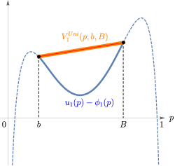
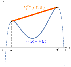
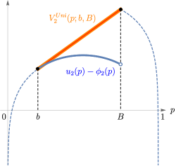
0.48 0.48 0.48 0.48

Figure 1: P1’s incentive under $[b,B]$.

Figure 2: P1’s incentive under $[b^{\prime},B^{\prime}]$.

Figure 3: P2’s incentive under $[b,B]$.

Figure 4: P2’s incentive under $[b^{\prime},B^{\prime}]$.

Figure 5: Illustrations of Equilibrium Characterization under Unilateral Stopping.

For unanimous stopping, first define an auxiliary payoff $v_{i}^{Una}$ that creates a “hole” within the sampling region $[\underline{p},\overline{p}]$ and otherwise equals $u_{i}-\phi_{i}$. Then construct the concave closure of $v_{i}^{Una}$ over $[0,1]$:

$$v^{Una}_{i}\left(p;\underline{p},\overline{p}\right)\mathrel{\mathop{\mathchar 58\relax}}= \left\{\begin{array}[]{ll}-\infty,&\text{for }p\in[\underline{p},\overline{p}],\\ u_{i}(p)-\phi_{i}(p),&\text{for }p\in[\underline{p},\overline{p}]^{c},\\ \end{array}\right.$$

$${V}_{i}^{Una}\left(p;\underline{p},\overline{p}\right)\mathrel{\mathop{\mathchar 58\relax}}= \sup\left\{z\mathrel{\mathop{\mathchar 58\relax}}(p,z)\in co(v_{i}^{Una})\right\},\text{ for }p\in[0,1].$$

See Figure 10 for graphical illustrations, in which blue curves are “modified” payoffs $v_{i}^{Una}$ and orange curves are concave closures $V_{i}^{Una}$. The “hole” within the graph of $v^{Una}_{i}$ is constructed to prohibit stopping within $[\underline{p},\overline{p}]$. Therefore, when $p_{t}=p$, $V_{i}^{Una}(p;\underline{p},\overline{p})$ captures the highest expected continuation payoff player $i$ can obtain by choosing an MPS of the binary policy with support $\{\underline{p},\overline{p}\}$—or equivalently, by prolonging the sampling process beyond $[\underline{p},\overline{p}]$.

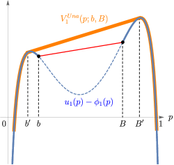
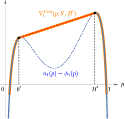
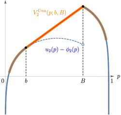
0.48 0.48 0.48 0.48

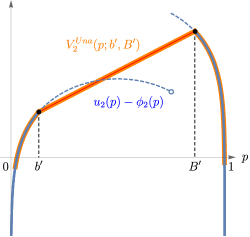
Figure 6: P1’s incentive under $[b,B]$.

Figure 7: P1’s incentive under $[b^{\prime},B^{\prime}]$.

Figure 8: P2’s incentive under $[b,B]$.

Figure 9: P2’s incentive under $[b^{\prime},B^{\prime}]$.

Figure 10: Illustrations of Equilibrium Characterization under Unanimous Stopping.

The following theorem presents equilibrium conditions using these concave closures.

Theorem 2 (Concavification).

A sampling region $[\underline{p},\overline{p}]$ with $\underline{p}\leq p_{0}\leq\overline{p}$ is an equilibrium outcome under unilateral (resp., unanimous) stopping if and only if for $i=1,2$,

$$\frac{\overline{p}-p_{0}}{\overline{p}-\underline{p}}[u_{i}(\underline{p})-\phi_{i}(\underline{p})]+\frac{p_{0}-\underline{p}}{\overline{p}-\underline{p}}[u_{i}(\overline{p})-\phi_{i}(\overline{p})]=V_{i}^{Uni}\left(p_{0};\underline{p},\overline{p}\right)\left(\text{resp., }{V}_{i}^{Una}\left(p_{0};\underline{p},\overline{p}\right)\right).$$ (1)

By the definition of concave closures, Equation 1 is equivalent to: for $\forall p\in[\underline{p},\overline{p}]$,

$$\frac{\overline{p}-p}{\overline{p}-\underline{p}}[u_{i}(\underline{p})-\phi_{i}(\underline{p})]+\frac{p-\underline{p}}{\overline{p}-\underline{p}}[u_{i}(\overline{p})-\phi_{i}(\overline{p})]=V_{i}^{Uni}\left(p;\underline{p},\overline{p}\right)\left(\text{resp., }{V}_{i}^{Una}\left(p;\underline{p},\overline{p}\right)\right).$$ (2)

Hence, the concave closures within the sampling region should be exactly given by the lines that connect payoffs at the boundary points of the sampling region.

Suppose that player $-i$ is using the sampling region $[\underline{p},\overline{p}]$, i.e., stopping immediately when $p_{t}$ escapes $[\underline{p},\overline{p}]$. Then, on the left-hand side of Equation 1, the linear combination of payoffs at the boundaries of $[\underline{p},\overline{p}]$ is player $i$’s expected payoff from also using this sampling region. Under unilateral stopping, players can only stop before each other and curtail the sampling process, so $V_{i}^{Uni}$ is the optimal payoff player $i$ can obtain; instead, under unanimous stopping, $V_{i}^{Una}$ is the best option available for player $i$, since now she can only stop after the other and prolong the sampling process. As a result, Equation 1 is simply the condition whereby using the equilibrium sampling region is optimal for players under unilateral or unanimous stopping, respectively.

See Figures 5 and 10 for graphical illustrations of equilibrium conditions under unilateral and unanimous stopping, respectively. The figures are drawn based on the same pair of players’ payoffs: $u_{1}-\phi_{1}$ is continuous, while $u_{2}-\phi_{2}$ is discontinuous but upper semi-continuous at point $B$. Let us consider two candidate sampling regions: $[b,B]$ and $[b^{\prime},B^{\prime}]$, where $[b,B]$ is player 2’s individually optimal sampling region and $[b^{\prime},B^{\prime}]$ is player 1’s. Therefore, we only need to ask whether player 1 has incentive to deviate from $[b,B]$ and similarly for $[b^{\prime},B^{\prime}]$ but with respect to player 2. Under unilateral stopping, the concave closure of player 1’s payoff within $[b,B]$, $V_{1}^{Uni}(p;b,B)$, is exactly given by the line that connects points $(b,u_{1}(b)-\phi_{1}(b))$ and $(B,u_{1}(B)-\phi_{1}(B))$, as shown in Figure 5. Therefore, player 1 always likes more information within $[b,B]$ and has no incentive to stop earlier. As a result, player 2’s individually optimal sampling region $[b,B]$ can be an equilibrium outcome under unilateral stopping. However, given player 1’s optimal sampling region $[b^{\prime},B^{\prime}]$, player 2 wants to stop immediately when $p_{t}$ hits or goes above $B$, as illustrated by the concave closure $V_{2}^{Uni}(p;b^{\prime},B^{\prime})$ in Figure 5. Therefore, $[b^{\prime},B^{\prime}]$ cannot be an equilibrium under unilateral stopping. Interestingly, the opposite is true under unanimous stopping: $[b^{\prime},B^{\prime}]$ can be an equilibrium outcome but $[b,B]$ cannot: by Figure 10, player 1 has incentive to learn more and extend player 2’s optimal sampling region $[b,B]$ to $[b^{\prime},B^{\prime}]$, so it is not an equilibrium; according to Figure 10, player 2 has no incentive to continue after $p_{t}$ leaves player 1’s optimal sampling region $[b^{\prime},B^{\prime}]$, hence it can be an equilibrium.

Maximum and Minimum Equilibria

Multiple sampling regions can satisfy the conditions in Theorem 2. I say an outcome $[\underline{p},\overline{p}]$ is larger than the other one $[\underline{p}^{\prime},\overline{p}{}^{\prime}]$, or $[\underline{p}^{\prime},\overline{p}{}^{\prime}]$ is smaller than $[\underline{p},\overline{p}]$, if $\underline{p}\leq\underline{p}^{\prime}$ and $\overline{p}\geq\overline{p}{}^{\prime}$. A binary policy associated with a larger sampling region is more informative than (or, a mean-preserving spread of) one associated with a smaller sampling region, i.e., players learn more with a larger sampling region. Therefore, largeness and informativeness induce the same partial order over sampling regions. Using equilibrium characterizations in Theorem 2, I show that equilibrium sampling regions under unilateral and unanimous stopping form a semi-lattice under this partial order.

Lemma 6.

Let $[\underline{p},\overline{p}]$ and $[\underline{p}^{\prime},\overline{p}{}^{\prime}]$ be two equilibrium sampling regions under unilateral (resp., unanimous) stopping. Then $\big{[}\min\{\underline{p},\underline{p}^{\prime}\},\max\{\overline{p},\overline{p}{}^{\prime}\}\big{]}$ (resp., $\big{[}\max\{\underline{p},\underline{p}^{\prime}\},\min\{\overline{p},\overline{p}{}^{\prime}\}\big{]}$) is also an equilibrium sampling region under unilateral (resp., unanimous) stopping.

Suppose that $\underline{p}\leq\underline{p}^{\prime}\leq p_{0}\leq\overline{p}\leq\overline{p}{}^{\prime}$. Consider the sampling region $[\underline{p},\overline{p}{}^{\prime}]$. Conditional on $p_{t}\in[\underline{p},\overline{p}]$, both players at least want to wait until the belief hits either $\underline{p}$ or $\overline{p}$, since $[\underline{p},\overline{p}]$ is an equilibrium outcome. Similarly, conditional on $p_{t}\in[\underline{p}^{\prime},\overline{p}{}^{\prime}]$, no one should have incentive to stop before the belief hits either $\underline{p}^{\prime}$ or $\overline{p}{}^{\prime}$. As a result, $[\underline{p},\overline{p}{}^{\prime}]$ is also an equilibrium outcome. The proof formalizes this intuition through the lens of Theorem 2.

As an implication of Lemma 6, there exists a maximum equilibrium outcome under unilateral stopping that is larger than all equilibrium sampling regions, and symmetrically a minimum equilibrium outcome under unanimous stopping that is smaller than all equilibrium sampling regions. Under unilateral stopping, for any two comparable equilibrium outcomes, the larger/more informative one is preferred by both players, since player $i$ has the choice to deviate to the smaller equilibrium outcome from the larger one but she does not want to do so. Therefore, under unilateral stopping, the maximum equilibrium outcome is the most preferred by both players among all equilibria and thus all other equilibria rely on players’ miscoordination. Symmetrically, under unanimous stopping, the minimum equilibrium outcome is the most preferred by both players.

When exploring comparative statics, to rule out the effect of equilibrium miscoordination, I focus on the maximum equilibrium outcome under unilateral stopping and the minimum one under unanimous stopping.

4.2 Inefficiencies and Conflicts of Interest

Pareto Inefficiencies

A natural question is how information acquisition is affected by players’ interactions compared to the single-agent case, and further whether collective information acquisition is efficient or not. To answer these questions, I compare equilibrium outcomes under unilateral and unanimous stopping with individually optimal outcomes and other Pareto efficient outcomes.

For any $\lambda=(\lambda_{1},\lambda_{2})\in\mathbb{R}_{+}^{2}$ such that $\lambda\neq\bm{0}=(0,0)$, define

$$W(p;\lambda)\mathrel{\mathop{\mathchar 58\relax}}=\lambda_{1}(u_{1}-\phi_{1})+\lambda_{2}(u_{2}-\phi_{2}).$$

Hence, $\mathbb{E}_{F}[W(p;\lambda)]$ is a weighted sum of players’ expected payoffs from a posterior distribution $F$. By concavifying $W(p;\lambda)$, we know that the maximum of $\mathbb{E}_{F}[W(p;\lambda)]$ (if it exists) over all Bayes plausible posterior distributions can be achieved using a binary policy which corresponds to a sampling region. Such a sampling region is $\lambda$-efficient.

Definition 3.

A sampling region $[\underline{p},\overline{p}]$ is $\bm{\lambda}$-efficient if its associated binary policy maximizes $\mathbb{E}_{F}[W(p;\lambda)]$ over all Bayes plausible posterior distributions.

When $\lambda_{i}>0$ and $\lambda_{-i}=0$, a $\lambda$-efficient sampling region captures player $i$’s optimal choice in an individual information acquisition problem. In general, $\lambda$-efficient sampling regions characterize all Pareto efficient sampling regions.

For simplicity, assume that the $\lambda$-efficient sampling region is unique for any $\lambda$, denoted by $[\underline{p}{}_{\lambda}^{*},\overline{p}{}_{\lambda}^{*}]$. By comparing equilibrium outcomes with $\lambda$-efficient sampling regions, I show that collective information acquisition is (weakly) Pareto inefficient: There is too little learning under unilateral stopping and too much learning under unanimous stopping.

Proposition 1 (Pareto Inefficiency).

Suppose that $[\underline{p}{}_{\lambda}^{*},\overline{p}{}_{\lambda}^{*}]$ is the unique $\lambda$-efficient sampling region for $\lambda\in\mathbb{R}_{+}^{2},\lambda\neq\bm{0}$. Any equilibrium outcome $[\underline{p},\overline{p}]$ under unilateral (resp., unanimous) stopping is smaller (resp., larger) than $[\underline{p}{}_{\lambda}^{*},\overline{p}{}_{\lambda}^{*}]$.

In particular, Proposition 1 implies that every player learns less under unilateral stopping compared to her individual optimum and learns more under unanimous stopping. Due to the nature of unilateral (resp., unanimous) stopping, equilibrium sampling regions can never be larger (resp., smaller) than the individual optimum, but in principle they may be not comparable. However, Proposition 1 claims that they are always comparable. Hence, under unilateral stopping the possibility that the other player may shut down learning on one side before it achieves player $i$’s optimum always urges player $i$ to stop earlier on the other side; and symmetric for unanimous stopping.

More notably, Proposition 1 shows that all equilibrium outcomes under unilateral (resp., unanimous) stopping are smaller (resp., larger) than all Pareto efficient ones, despite that Pareto efficient outcomes may intersect with each other.

That equilibrium outcomes are always comparable to Pareto efficient outcomes is due to the semi-lattice structure of equilibrium outcomes we identified in Lemma 6. Fix a weight $\lambda\in\mathbb{R}_{+}^{2}\setminus\{\bm{0}\}$. Let us consider an auxiliary game between two virtual players withe the same preference $W(p;\lambda)=\lambda_{1}(u_{1}-\phi_{1})+\lambda_{2}(u_{2}-\phi_{2})$. If $[\underline{p},\overline{p}]$ is an equilibrium outcome under unilateral stopping between players with preferences $u_{i}-\phi_{i}$, it should also be an equilibrium in the auxiliary game; otherwise, either player 1 or 2 has strict incentive to deviate in the original game. By definition, the $\lambda$-efficient $[\underline{p}{}_{\lambda}^{*},\overline{p}{}_{\lambda}^{*}]$ is another equilibrium outcome. Then according to Lemma 6, $[\min\{\underline{p},\underline{p}{}_{\lambda}^{*}\},\max\{\overline{p},\overline{p}{}_{\lambda}^{*}\}]$ is also an equilibrium in the auxiliary game. Since $[\underline{p}{}_{\lambda}^{*},\overline{p}{}_{\lambda}^{*}]$ is uniquely optimal for preference $W$, it must be $\min\{\underline{p},\underline{p}{}_{\lambda}^{*}\}=\underline{p}{}_{\lambda}^{*}$ and $\max\{\overline{p},\overline{p}{}_{\lambda}^{*}\}=\overline{p}{}_{\lambda}^{*}$, and thus $[\underline{p},\overline{p}]$ is smaller than $[\underline{p}{}_{\lambda}^{*},\overline{p}{}_{\lambda}^{*}]$.

Impact of Conflicts of Interest

Given the learning inefficiency results in Proposition 1, a natural question is how the inefficiency is affected by players’ conflicts of interest. We expect the inefficiency to be amplified when players’ preferences become less aligned. This intuition is formalized as follows.

Suppose that there are two functions $f$ and $g$ over posteriors such that players’ terminal payoffs take the following form:

$$u_{1}(p)=f(p)+bg(p)\quad\text{and}\quad u_{2}(p)=f(p)-bg(p),$$

where $b\geq 0$ captures the extent of preference misalignment between two players. Let $T^{b}$ denote the set of all equilibrium outcomes when misalignment is $b$.

Lemma 7.

Suppose that $c_{1}(\cdot)=c_{2}(\cdot)$. Then $T^{b}\subset T^{b^{\prime}}$ for any $b>b^{\prime}\geq 0$.

The intuition behind Lemma 7 is as follows: When preferences are less aligned, there are fewer outcomes that both players do not want to deviate from. Given Lemmas 6 and 7, the following result ensues.

Proposition 2 (Increased Misalignment).

Suppose that $c_{1}(\cdot)=c_{2}(\cdot)$. As misalignment $b$ increases, the maximum equilibrium outcome under unilateral stopping becomes smaller, and the minimum equilibrium outcome under unanimous stopping becomes larger.

It is worth noticing that all comparisons in this section are in a weak sense.

4.3 General Collective Stopping Rules with $n\geq 2$ Players

Although I focus on the two-player case in the baseline framework, the method I present can easily extend to the situation with more players under general collective stopping rules. Let $N$ be the set of players and $C$ denote a generic subset of $N$.

Definition 4.

For any collection of non-empty subsets of $N$, denoted by $\mathcal{C}$, under the $\mathcal{C}$-collective stopping rule, information acquisition ends whenever there is a subset of players $C\in\mathcal{C}$ such that all players in $C$ have stopped.

If $\mathcal{C}$ contains all singletons, then the $\mathcal{C}$-collective stopping rule corresponds to unilateral stopping; if $\mathcal{C}=\{N\}$, it is unanimous stopping. In general, if $\mathcal{C}=\mathcal{C}^{q}\mathrel{\mathop{\mathchar 58\relax}}=\{C\subset N\mathrel{\mathop{\mathchar 58\relax}}|C|\geq q\}$ for $q\in\{1,\dots,|N|\}$, information acquisition is terminated whenever $q$ players have stopped. This is a typical quota rule in the collective-choice literature, which I call the $q$-collective stopping rule.

Definition 5.

For any $q\in\{1,\dots,n\}$, under the $\boldsymbol{q}$-collective stopping rule, information acquisition ends whenever $q$ players have stopped.

$\mathcal{C}$-collective stopping rules can also capture rules without anonymity. For example, in some contexts, there is a “chairperson” among players such that information acquisition ends when a majority stops as long as the majority includes the chairperson. This situation can be modeled by a $\mathcal{C}$-collective stopping rule with $\mathcal{C}=\mathcal{C}^{q}\cap\mathcal{N}_{i}$ where $i$ is the chairperson and $\mathcal{N}_{i}\mathrel{\mathop{\mathchar 58\relax}}=\{C\subset N\mathrel{\mathop{\mathchar 58\relax}}i\in C\}$.

Suppose that the $\mathcal{C}$-collective stopping rule governs the termination of information acquisition. Let $\bm{\tau}\mathrel{\mathop{\mathchar 58\relax}}=(\tau_{j})_{j\in N}$ denote the profile of players’ individual stopping times, and $\bm{\tau}_{-i}\mathrel{\mathop{\mathchar 58\relax}}=(\tau_{j})_{j\in N\backslash\{i\}}$ denote stopping times by all players other than $i$. Given players’ stopping times $\bm{\tau}$, under the $\mathcal{C}$-collective stopping rule, information acquisition ends at time $\tau^{\mathcal{C}}(\bm{\tau})\mathrel{\mathop{\mathchar 58\relax}}=\min_{C\in\mathcal{C}}\max_{j\in C}\tau_{j}$.

Fix an arbitrary player $i$. Let $\mathcal{C}_{i}\mathrel{\mathop{\mathchar 58\relax}}=\{C\in\mathcal{C}\mathrel{\mathop{\mathchar 58\relax}}i\in C\}$, so $\mathcal{C}\backslash\mathcal{C}_{i}$ is the collection of subsets in $\mathcal{C}$ that do contain player $i$. Define $\mathcal{C}-\{i\}\mathrel{\mathop{\mathchar 58\relax}}=\{C\backslash\{i\}\mathrel{\mathop{\mathchar 58\relax}}C\in\mathcal{C}\}$ to be the result derived by subtracting $i$ from all subsets in $\mathcal{C}$. By definition, $\mathcal{C}\backslash\mathcal{C}_{i}\subset\mathcal{C}-\{i\}$. Notice that $C\subset N\backslash\{i\}$ for any $C\in\mathcal{C}-\{i\}$, thus $\mathcal{C}\backslash\mathcal{C}_{i}$ and $\mathcal{C}_{i}\subset\mathcal{C}-\{i\}$ induce collective stopping rules when the set of players is restricted to $N\backslash\{i\}$. Consider $\tau^{\mathcal{C}-\{i\}}(\bm{\tau}_{-i})\mathrel{\mathop{\mathchar 58\relax}}=\min_{C\in\mathcal{C}-\{i\}}\max_{j\in C}\tau_{j}$ where $\max_{j\in C}\tau_{j}\mathrel{\mathop{\mathchar 58\relax}}=0$ for $C=\emptyset$, and $\tau^{\mathcal{C}\backslash\mathcal{C}_{i}}(\bm{\tau}_{-i})\mathrel{\mathop{\mathchar 58\relax}}=\min_{C\in\mathcal{C}\backslash\mathcal{C}_{i}}\max_{j\in C}\tau_{j}$ where $\tau^{\mathcal{C}\backslash\mathcal{C}_{i}}(\bm{\tau}_{-i})\mathrel{\mathop{\mathchar 58\relax}}=\infty$ if $\mathcal{C}\backslash\mathcal{C}_{i}=\emptyset$. By definition, $\tau^{\mathcal{C}-\{i\}}(\bm{\tau}_{-i})\leq\tau^{\mathcal{C}\backslash\mathcal{C}_{i}}(\bm{\tau}_{-i})$. Given $\bm{\tau}_{-i}$, information acquisition will end at time $\tau^{\mathcal{C}-\{i\}}(\bm{\tau}_{-i})$ if player $i$ stops at the very beginning; it will end at time $\tau^{\mathcal{C}\backslash\mathcal{C}_{i}}(\bm{\tau}_{-i})$ if player $i$ never stops. Hence, by adjusting her stopping time $\tau_{i}$, player $i$ can choose to terminate information acquisition at any time between $\tau^{\mathcal{C}-\{i\}}(\bm{\tau}_{-i})$ and $\tau^{\mathcal{C}\backslash\mathcal{C}_{i}}(\bm{\tau}_{-i})$. According to Lemmas 3, 2 and 4, player $i$ can thus choose posterior distributions that are MPS of $F_{\tau^{\mathcal{C}-\{i\}}(\bm{\tau}_{-i})}$ and also MPC of $F_{\tau^{\mathcal{C}\backslash\mathcal{C}_{i}}(\bm{\tau}_{-i})}$. Therefore, the problem is a hybrid of the ones under unilateral and unanimous stopping.

When $\bm{\tau}_{-i}$ are all Markov stopping times, $F_{\tau^{\mathcal{C}-\{i\}}(\bm{\tau}_{-i})}$ and $F_{\tau^{\mathcal{C}\backslash\mathcal{C}_{i}}(\bm{\tau}_{-i})}$ are binary policies that can be represented by nested sampling regions, denoted by $[\underline{p}^{\mathcal{C}-\{i\}}(\bm{\tau}_{-i}),\overline{p}^{\mathcal{C}-\{i\}}(\bm{\tau}_{-i})]$ and $[\underline{p}^{\mathcal{C}\backslash\mathcal{C}_{i}}(\bm{\tau}_{-i}),\overline{p}^{\mathcal{C}\backslash\mathcal{C}_{i}}(\bm{\tau}_{-i})]$ with $\underline{p}^{\mathcal{C}\backslash\mathcal{C}_{i}}\leq\underline{p}^{\mathcal{C}-\{i\}}\leq\overline{p}^{\mathcal{C}-\{i\}}\leq\overline{p}^{\mathcal{C}\backslash\mathcal{C}_{i}}$. Therefore, player $i$ can effectively choose any sampling region larger than $[\underline{p}^{\mathcal{C}-\{i\}}(\bm{\tau}_{-i}),\overline{p}^{\mathcal{C}-\{i\}}(\bm{\tau}_{-i})]$ but smaller than $[\underline{p}^{\mathcal{C}\backslash\mathcal{C}_{i}}(\bm{\tau}_{-i}),\overline{p}^{\mathcal{C}\backslash\mathcal{C}_{i}}(\bm{\tau}_{-i})]$. We can thus study players’ incentive and derive equilibrium conditions via concavification, similar to what is presented in Theorem 2.

5 Applications

In this section, I apply the general framework developed in the previous section to three problems: committee search, dynamic persuasion, and competition in persuasion. First, I illustrate in detail how to analyze the multiplayer situation under $q$-collective stopping rules using the committee search setup. Then, in the other applications, I show how the equilibrium characterizations in Theorems 1 and 2 can be used to derive intriguing insights in different economic contexts.

5.1 Committee Search

A committee of $2m-1$ ($m\geq 2$ is an integer) players decides between two alternatives, $\alpha$ and $\beta$. The payoff from each alternative depends on an underlying binary state $\theta\in\Theta=\{0,1\}$. Players share a common prior about the state given by $p_{0}=\mathbb{P}(\theta=1)\in(0,1)$. In state $\theta=0$, player $i$’s payoff from $\alpha$ is 1 and her payoff from $\beta$ is 0. In state $\theta=1$, player $i$’s payoff from $\alpha$ is 0 and her payoff from $\beta$ is $v_{i}\geq 0$. Assume that players are heterogeneous, with $v_{1}<\cdots<v_{i}<\cdots<v_{2m-1}$. Hence, players’ preferences are aligned: They prefer $\alpha$ in state $\theta=0$ and $\beta$ in state $\theta=1$; however, they differ in the intensity of their preferences: Player $i$ prefers $\beta$ if and only if her belief about $\theta=1$ is high, i.e., $p\geq 1/(1+v_{i})=\mathrel{\mathop{\mathchar 58\relax}}t_{i}$, where $t_{i}$ refers to player $i$’s individual belief threshold. Players’ preferences are common knowledge.

In the committee, a collective decision is made via voting. Before entering the voting, players can search for public information and update their beliefs. As in the baseline framework, the searching/information acquisition process is represented by a public belief process $(p_{t})_{t\geq 0}$ that satisfies Assumption 1. Players bear flow costs $c_{i}(p_{t})\geq 0$ during information acquisition and decide when to stop this process under the $\boldsymbol{q}$-collective stopping rule introduced in Section 4.3, for $q\in\{1,\dots,2m-1\}$. At the end of information acquisition, player $i$ obtains a payoff of $u_{i}(p)=1-p$ when $p$ when $p<t_{l}$ and $u_{i}(p)=pv_{i}$ when $p\geq t_{l}$ for some $l\in\{m,\dots,2m-1\}$.

Recall that under the $q$-collective stopping rule, information acquisition is terminated whenever $q$ players have stopped. When $q\geq m$, $q$-collective stopping captures the situation in which continuing information acquisition is the status quo and stopping requires a (super-)majority of votes in a committee. When $q<m$, the status quo is instead stopping and continuing requires a (super-)majority of votes.

Equilibrium, Refinement, and One-sided Best Responses

For simplicity, I only consider pure-strategy Markov perfect equilibrium (PSMPE), so that players’ stopping strategies can be represented by sampling intervals $[\underline{p}{}_{i},\overline{p}{}_{i}]$ with $\underline{p}{}_{i}\leq p_{0}\leq\overline{p}{}_{i}$—i.e., player $i$ stops immediately when the public belief $p_{t}$ hits either $\underline{p}{}_{i}$ or $\overline{p}{}_{i}$. Let $\sigma_{i}=(\underline{p}{}_{i},\overline{p}{}_{i})$ denote player $i$’s stopping strategy and $\sigma_{-i}$ the collection of all other players’ strategies. For any strategy profile $\sigma=(\sigma_{1},\dots,\sigma_{2m-1})$, let $\underline{p}^{k}(\sigma)$ denote the $k$-th largest $\underline{p}{}_{i}$ in $\sigma$ and $\overline{p}{}^{k}(\sigma)$ denote the $k$-th smallest $\overline{p}{}_{i}$ in $\sigma$ with $\underline{p}^{0}=\overline{p}{}^{0}=p_{0}$; moreover, let $\underline{p}{}^{k}_{-i}(\sigma_{-i})$ denote the $k$-th largest $\underline{p}{}_{j}$ in $\sigma_{-i}$ and $\overline{p}{}^{k}_{-i}(\sigma_{-i})$ denote the $k$-th smallest $\overline{p}_{j}$ in $\sigma_{-i}$. When there is no confusion, I suppress the dependence of $\underline{p}^{k},\overline{p}{}^{k},\underline{p}{}^{k}_{-i},\overline{p}{}^{k}_{-i}$ on $\sigma$ or $\sigma_{-i}$ for expositional simplicity. Given strategy profile $\sigma$, under the $q$-collective stopping rule, information acquisition ends whenever $p_{t}$ hits $\underline{p}^{q}$ or $\overline{p}{}^{q}$, so the resulting sampling region is $[\underline{p}^{q},\overline{p}{}^{q}]$. According to Lemma 5, when the sampling region is $[\underline{p},\overline{p}]$, player $i$’s expected payoff is given by

$$U_{i}\left(\underline{p},\overline{p};p_{0}\right)\mathrel{\mathop{\mathchar 58\relax}}=\frac{\overline{p}-p_{0}}{\overline{p}-\underline{p}}[u_{i}(\underline{p})-\phi_{i}(\underline{p})]+\frac{p_{0}-\underline{p}}{\overline{p}-\underline{p}}[u_{i}(\overline{p})-\phi_{i}(\overline{p})],$$

where $\phi_{i}$ is defined by Equation 1 in Lemma 5. Therefore, player $i$’s expected payoff under strategy profile $\sigma$ is $U_{i}(\underline{p}^{q},\overline{p}{}^{q};p_{0})$.

As discussed in Section 4.3, when all other players use Markov stopping times $\bm{\tau}_{-i}$, under the $\mathcal{C}$-collective stopping rule, player $i$ can choose among sampling regions larger than $[\underline{p}^{\mathcal{C}-\{i\}}(\bm{\tau}_{-i}),\overline{p}^{\mathcal{C}-\{i\}}(\bm{\tau}_{-i})]$ and smaller than $[\underline{p}^{\mathcal{C}\backslash\mathcal{C}_{i}}(\bm{\tau}_{-i}),\overline{p}^{\mathcal{C}\backslash\mathcal{C}_{i}}(\bm{\tau}_{-i})]$. When $\mathcal{C}=\mathcal{C}^{q}$ and when $\bm{\tau}_{-i}$ are characterized by sampling intervals $\sigma_{-i}$, $[\underline{p}^{\mathcal{C}-\{i\}}(\bm{\tau}_{-i}),\overline{p}^{\mathcal{C}-\{i\}}(\bm{\tau}_{-i})]=[\underline{p}{}_{-i}^{q-1},\overline{p}^{q-1}_{-i}]$ and $[\underline{p}^{\mathcal{C}\backslash\mathcal{C}_{i}}(\bm{\tau}_{-i}),\overline{p}^{\mathcal{C}\backslash\mathcal{C}_{i}}(\bm{\tau}_{-i})]=[\underline{p}{}_{-i}^{q},\overline{p}^{q}_{-i}]$. In other words, under the $q$-collective stopping rule, player $i$ has to be the pivotal person if she wants to change the collective sampling region. Hence, $\sigma$ is a PSMPE under the $q$-collective stopping rule if

$$U_{i}\left(\underline{p}^{q},\overline{p}{}^{q};p_{0}\right)\geq U_{i}\left(\underline{p},\overline{p};p_{0}\right),\forall\underline{p}\in\left[\underline{p}{}_{-i}^{q},\underline{p}{}_{-i}^{q-1}\right],\forall\overline{p}\in\left[\overline{p}{}^{q-1}_{-i},\overline{p}{}^{q}_{-i}\right],\forall i. q$$ (-collective)

Note that ($q$-collective) can be rewritten as a concavification condition similar to the one presented in Theorem 2. However, this condition is trivially satisfied for $1<q<2m-1$ when all other players use the same stopping strategy in which case $\underline{p}^{q}=\underline{p}{}_{-i}^{q}=\underline{p}{}_{-i}^{q-1}$ and $\overline{p}{}^{q}=\overline{p}{}^{q-1}_{-i}=\overline{p}{}^{q}_{-i}$. As a result, all the players using the same stopping strategy is always an equilibrium under $q$-collective stopping rule for $1<q<2m-1$. To rule out such trivial equilibria which commonly arise in voting games, I introduce additional requirements on equilibrium profiles, called one-sided best responses.

For any equilibrium sampling region $[\underline{p}^{q},\overline{p}{}^{q}]$, define

$$\overline{B}_{i}(\underline{p}^{q})\mathrel{\mathop{\mathchar 58\relax}}=\operatorname*{argmax}_{\overline{p}\geq p_{0}\vee t_{l}}U_{i}\left(\underline{p}^{q},\overline{p};p_{0}\right)$$

and

$$\underline{B}{}_{i}(\overline{p}{}^{q})\mathrel{\mathop{\mathchar 58\relax}}=\operatorname*{argmax}_{\underline{p}\leq p_{0}\wedge t_{l}}U_{i}\left(\underline{p},\overline{p}{}^{q};p_{0}\right).$$

Given $\underline{p}^{q}$ fixed, which is the point at which the committee stops searching and chooses $\alpha$, $\overline{B}_{i}(\underline{p}^{q})$ describes player $i$’s optimal choice—or one-sided best response—if she can decide when the committee stops and chooses $\beta$. Similarly, $\underline{B}{}_{i}(\overline{p}{}^{q})$ is player $i$’s one-sided best response to $\overline{p}{}^{q}$ if she can decide when the committee stops and chooses $\alpha$ with $\overline{p}{}^{q}$ fixed. When $c_{i}(p)>0$ and thus $\phi_{i}$ is strictly convex, both $\overline{B}_{i}(\underline{p}^{q})$ and $\underline{B}{}_{i}(\overline{p}{}^{q})$ are singletons.

My equilibrium refinement is introduced based on these one-sided best responses.

Definition 6.

An equilibrium $\sigma$ under the $q$-collective stopping rule has one-sided best responses (OSBR) if $\overline{p}{}_{i}\in\overline{B}_{i}(\underline{p}^{q})$ and $\underline{p}{}_{i}\in\underline{B}{}_{i}(\overline{p}{}^{q})$ for all $i$.

The requirement for one-sided best responses can be motivated as follows: When players evaluate when to stop and vote for one alternative, they take the circumstances under which the other alternative will be selected as given. This refinement can also be justified by requiring equilibrium strategies to be (one-sided) undominated for all players; see Appendix C. As we will see later, the maximum (resp., minimum) equilibrium outcome under unilateral (resp., unanimous) stopping survives this refinement.

Learning in Symmetric Committees

To simplify the analysis, consider the simplest case in which players are homogeneous in sampling costs, i.e., $c_{i}(p)=c(p)>0$ for all $i$ and $p\in[0,1]$. Since $\phi_{i}=\phi$ is strictly convex for all $i$, one-sided best responses are unique (both $\overline{B}_{i}(\underline{p})$ and $\underline{B}{}_{i}(\overline{p})$ are singletons). Monotone comparative statics can verify that both $\overline{B}_{i}(\underline{p})$ and $\underline{B}{}_{i}(\overline{p})$ are decreasing in $i$.

Given this ordering structure, in equilibrium it must be $\overline{p}{}^{q}=\overline{B}_{2m-q}(\underline{p}^{q})$ and $\underline{p}^{q}=\underline{B}{}_{q}(\overline{p}{}^{q})$. This is not only necessary but also sufficient. Therefore, it suffices to focus on the interaction between player $2m-q$ and player $q$. These two players are pivotal in determining the upper bound and the lower bound of the sampling region, respectively. When $q\geq m$, $\overline{B}_{2m-q}\geq\overline{B}_{q}$ and $\underline{B}{}_{q}\leq\underline{B}{}_{2m-q}$, so $\overline{p}{}^{q}=\overline{B}_{2m-q}(\underline{p}^{q})$ and $\underline{p}^{q}=\underline{B}{}_{q}(\overline{p}{}^{q})$ capture the situation under unanimous stopping between player $2m-q$ and player $q$. When $q\leq m$, it is instead unilateral stopping between these two players.

The following proposition summarizes the above observations.

Proposition 3.

Suppose that players are homogeneous in sampling costs. A sampling region $[\underline{p},\overline{p}]$ is an equilibrium outcome with OSBR under the $q$-collective stopping rule if and only if it is an equilibrium outcome with OSBR under unanimous stopping between player $q$ and player $2m-q$ when $q\geq m$, but under unilateral stopping between player $q$ and player $2m-q$ when $q\leq m$.

All proofs in Section 5 are relegated to Appendix B.

Therefore, the existence of equilibrium with OSBR under $q$-collective stopping can be established by showing the existence of equilibrium with OSBR under unilateral or unanimous stopping between player $q$ and player $2m-q$.

Lemma 8.

When $q<m$, the maximum equilibrium under unilateral stopping between player $q$ and player $2m-q$ has OSBR. When $q\geq m$, the minimum equilibrium under unanimous stopping between these two players also has OSBR.

Also, thanks to the reduction in Proposition 3, we can extend the previous results on learning inefficiency in the two-player case to the committee search setup. To this end, consider symmetric committees:

Definition 7.

A committee is symmetric if $v_{m-k}+v_{m+k}=2v_{m}$ for any $k\in\{1,\dots,m-1\}$ and $c_{i}(p)=c(p)>0$ for any $i\in\{1,\dots,2m-1\}$.

A symmetric committee is more diverse if, for any $k\in\{1,\dots,m-1\}$, $v_{m-k}$ decreases and $v_{m+k}$ increases by the same amount.

Define social welfare as the sum of all players’ expected payoffs. In a symmetric committee, the socially optimal sampling region coincides with the optimal one for player $m$ as well as the optimal one for the pair of player $m-k$ and player $m+k$ for any $k\in\{1,\dots,m-1\}$. Therefore, the following result for learning inefficiency under $q$-collective stopping rules in symmetric committees can easily be obtained as a corollary of Propositions 1 and 3: From the perspective of social welfare, $q$-collective stopping rules lead to too little learning when $q<m$ and too much learning when $q>m$.

Corollary 1.

Let $[\underline{p}^{*},\overline{p}{}^{*}]$ denote the unique socially optimal sampling region. In a symmetric committee, any equilibrium outcome with OSBR $[\underline{p},\overline{p}]$ under the $q$-collective stopping rule is smaller than $[\underline{p}^{*},\overline{p}{}^{*}]$ when $q\leq m$, but larger than $[\underline{p}^{*},\overline{p}{}^{*}]$ when $q\geq m$.

More interestingly, when $q<m$ and when $q>m$, increasing the diversity (misalignment) of a committee has opposite effects on learning outcomes. Notice that in a symmetric committee, $u_{i}(p)=u_{m}(p)+(v_{i}-v_{m})p\mathbbm{1}_{p\geq t_{l}}$ and $(v_{q}-v_{m})=-(v_{2m-q}-v_{m})$, and therefore Proposition 2 is applicable, whereby both an increase in $q$ and an increase in diversity can be viewed as an increase in misalignment $b\mathrel{\mathop{\mathchar 58\relax}}=v_{q}-v_{m}$.

Let $[\underline{p},\overline{p}]$ denote the maximum (resp., minimum) equilibrium sampling region with OSBR under the $q$-collective stopping rule when $q>m$ (resp., $q<m$). I say learning becomes longer if $[\underline{p},\overline{p}]$ becomes larger, i.e., if $\underline{p}$ decreases and $\overline{p}$ increases.

Corollary 2.

In a symmetric committee:

• As $q$ increases, learning always becomes longer.

• As the committee becomes more diverse, learning becomes shorter when $q<m$ and longer when $q>m$.

Recall that $q$-collective stopping rules with $q<m$ can be interpreted as super-majority voting to continue information acquisition with stopping as the status quo. In contrast, $q$-collective stopping rules with $q>m$ are super-majority voting to stop searching with continuing as the status quo. Thus, an implication of Corollaries 1 and 2 is that under super-majority rules, voting to continue information acquisition leads to too little learning from the perspective of social welfare, whereby a higher majority requirement or a more diverse committee further shortens learning; in contrast, voting to stop results in too much learning, and learning becomes longer with a higher majority requirement or in a more diverse committee.

Connection to Chan, Lizzeri, Suen and Yariv (2018)

This application of committee search is similar to the model of deliberation in committees studied by Chan et al. (2018). Except for some mathematical differences (e.g., discounting vs. flow costs), conceptually Chan et al. (2018) mainly focus on what they call the “one-stage process” in which the deliberation (i.e., sampling) stage and the decision stage are linked together and they only consider (super-)majority rules (i.e., $q$-collective stopping rules with $q\geq m$). My model features a separation between deliberation and decision, and thus I consider the “two-stage process” defined in their paper; in addition, I study “minority” deliberation/stopping rules with $q<m$. My results for the two-stage process with $q\geq m$ in Corollaries 1 and 2 are consistent with Chan et al.’s (2018) findings for the one-stage process, but my new results for $q<m$ demonstrate opposite patterns.

In terms of methodologies, Chan et al. (2018) use dynamic programming and solve a differential equation, while my analysis is based on the concavification method developed in the baseline framework. The concavification approach only cares about the geometric properties of indirect payoffs and the impact of their changes on the set of equilibrium outcomes when studying comparative statics. Hence, it enables me to accommodate general belief processes and also helps me avoid the direct investigation on comparative statics of the fixed points of one-sided best responses, which can be complicated since the committee search game I studied is not supermodular.

5.2 Dynamic Persuasion

The second application concerns a dynamic persuasion game between a Sender (S, “he”) and a Receiver (R, “she”). R faces a decision problem with a finite action space $A$. Players’ payoffs from each action depend on an unknown binary state $\theta\in\Theta=\{0,1\}$, given by $u_{R}^{0}\mathrel{\mathop{\mathchar 58\relax}}A\times\Theta\to\mathbb{R}$ and $u_{S}^{0}\mathrel{\mathop{\mathchar 58\relax}}A\times\Theta\to\mathbb{R}$. Players are Bayesian and share a common prior about the state $p_{0}=\mathbb{P}(\theta=1)\in(0,1)$. Before R makes a decision, S can persuade her by dynamically collecting and disclosing public information about the state. As in the baseline framework, the dynamic persuasion process is modeled by a public belief process $(p_{t})_{t\geq 0}$ that satisfies Assumption 1. Players bear flow costs $c_{i}(p_{t})\geq 0$ during persuasion and decide when to stop persuasion under unilateral stopping: R can stop listening to S and make the decision at any time, and S can also stop persuading at any time; moreover, S’s stopping is irreversible. In a later exercise in Section 5.2.2, I explore the situation in which S’s stopping is reversible and thus S can restart persuasion. When persuasion is finished, R chooses an action to maximize her expected payoff given her posterior belief about the state.

Let $p$ denote a generic posterior belief about $\theta=1$ when persuasion is finished. Let $a(p)\in\arg\max_{a\in A}pu_{R}^{0}(a,1)+(1-p)u_{R}^{0}(a,0)$ denote R’s optimal decision under posterior $p$, where $a(p)$ is selected to be the sender-preferred action upon R’s indifference. Define $u_{i}(p)\mathrel{\mathop{\mathchar 58\relax}}=pu_{i}^{0}(a(p),1)+(1-p)u_{i}^{0}(a(p),0)$ for $i=R,S$. Since $A$ is finite, $u_{i}$ is piecewise linear, Lebesgue measurable, and bounded. Moreover, $u_{R}$ is continuous and convex, and $u_{S}$ is upper semicontinuous. To make the persuasion problem nontrivial, assume that (i) there is no dominant action for R that is optimal in both states, and that (ii) neither R nor S is indifferent across all the actions in $\{a(p)\}_{p\in[0,1]}$. As a result, neither $u_{R}$ nor $u_{S}$ is linear.

5.2.1 Dynamic Persuasion and Bayesian Persuasion

This section focuses on the case in which S’s stopping is irreversible. Therefore, characterizations in Theorems 1 and 2 for unilateral stopping are applicable to this dynamic persuasion game. Using these results, I establish a connection between dynamic persuasion problems and the static Bayesian persuasion problems studied by Kamenica and Gentzkow (2011).

Consider the standard Bayesian persuasion problem in Kamenica and Gentzkow (2011): S chooses a Bayes plausible posterior distribution $F$ to maximize $\mathbb{E}_{F}[u_{S}]$. Let $F_{KG}$ denote the solution(s) to this Bayesian persuasion problem (KG solution(s) hereafter). The following result shows that dynamic persuasion can happen in equilibrium with sufficiently small sampling costs, in a weak sense, “if and only if” the KG solution $F_{KG}$ is of strictly positive information value for both players, i.e., $\mathbb{E}_{F_{KG}}[u_{i}]>u_{i}(p_{0})$. In a sense, the KG solution being of zero information value for one player but not the other captures the situation where players’ preferences are very misaligned, which tends to result in inefficiently short learning under unilateral stopping.

Proposition 4.

Suppose that the sender’s stopping is irreversible.

• If all KG solutions are of zero information value for the receiver, then for any $c_{S},c_{R}>0$ the only Nash equilibrium outcome in the dynamic persuasion game is that players stop immediately, i.e., no persuasion.

• If the KG solution is unique and has strictly positive information value for both the sender and the receiver, then this solution can be a PSMPE outcome in the dynamic persuasion game under some sufficiently small $c_{S},c_{R}>0$.

The intuition for part (b) is straightforward: When sampling costs vanish, R is always willing to listen until S stops (since $u_{R}$ is convex). Therefore, as characterized by Problem (3), S faces approximately a standard Bayesian persuasion problem with $u_{S}$, in which it is optimal to implement the KG solution.

The idea of part (a) is illustrated by the following corollary. When $|A|=2$, S’s preference being state-independent is a sufficient condition for the KG solutions to have no information value for R, and thus invokes part (a) of Proposition 4.

Corollary 3 (Persuasion failure when $|A|=2$).

Suppose that the sender’s stopping is irreversible. If $c_{S},c_{R}>0$, $|A|=2$, and $u^{0}_{S}(a,0)=u^{0}_{S}(a,1)$ for all $a\in A$, then the only Nash equilibrium outcome in the dynamic persuasion game is that players stop immediately.

Corollary 3 can be graphically illustrated by Figure 13. Let $A=\{a_{-},a_{+}\}$ and let $\hat{p}\in(0,1)$ denote the belief threshold such that R prefers $a_{+}$ if and only if $p\geq\hat{p}$. Given that S’s preference is state-independent, without loss suppose that S strictly prefers $a_{+}$ to $a_{-}$. Since $c_{i}>0$, $\phi_{i}$ is strictly convex and thus $u_{i}-\phi_{i}$ is concave below $\hat{p}$ and above $\hat{p}$, respectively. Let $[\underline{p},\overline{p}]$ be an equilibrium sampling region in some PSMPE. Suppose that players do not stop immediately, so $\underline{p}<p_{0}<\overline{p}$. On the one hand, if the sampling region does not cross $\hat{p}$, the concavification condition in Theorem 2 under unilateral stopping fails for R, as shown in Figure 13; on the other hand, if the sampling region does cross $\hat{p}$, according to Figure 13, the concavification condition fails for S. As a result, players must stop immediately in any PSMPE. This is also true for NE.

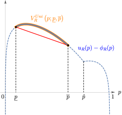
0.48 0.48

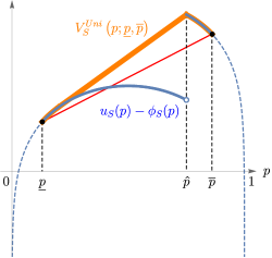
Figure 11: R’s incentive when $[\underline{p},\overline{p}]$ does not cross $\hat{p}$.

Figure 12: S’s incentive when $[\underline{p},\overline{p}]$ does cross $\hat{p}$.

Figure 13: Illustration of Persuasion Failure.

In terms of the intuition, notice that S has no incentive to continue costly persuasion whenever $p_{t}\geq\hat{p}$, i.e., whenever R is already willing to choose $a_{+}$. Anticipating that S will stop providing information whenever the belief reaches $\hat{p}$, at which point R is indifferent between two actions, R has no incentive to wait since the ex ante information value is zero for her but she needs to bear waiting costs. The same logic extends to the general payoff structures specified in part (a): If $F_{KG}$ is of zero value for R, then observing a signal from $F_{KG}$, either R still finds $a(p_{0})$ to be optimal or she changes her decision to $a^{\prime}$ but is indifferent between $a(p_{0})$ and $a^{\prime}$. Since $F_{KG}$ is optimal for S when there is no cost, S has no incentive to persuade R to take action other than $a(p_{0})$ or $a^{\prime}$ and more importantly, he has no incentive to continue costly persuasion whenever $p_{t}$ hits the point at which R is indifferent between $a(p_{0})$ and $a^{\prime}$. Anticipating this, R will stop immediately since she cannot benefit from listening to persuasion.

According to Figure 13, when sampling costs are small, the no persuasion outcome is strictly Pareto dominated by an outcome in which S continues persuasion slightly beyond the threshold $\hat{p}$—both S and R can strictly benefit from “longer persuasion.”

In addition to these general results, when players’ preferences can be written as $u_{R}(p)=f(p)+bg(p)$ and $u_{S}(p)=f(p)-bg(p)$ with two functions $f,g$ and a parameter $b\geq 0$, according to Proposition 2, we can show that an increase in misalignment $b$ leads to shorter persuasion or less information revealed.

5.2.2 When the Sender’s Stopping is Reversible: “Anything Goes”

In the previous analysis, I assume that S’s stopping of persuasion is irreversible and thus S can credibly threaten to provide no information in the future by stopping. This assumption can be justified by the prohibitively high costs of switching regimes in some economic contexts (e.g., it may be too costly for drug firms to restart clinical trials after abandoning them). However, in other situations, S can always restart persuasion as long as R has not made a decision, so his stopping is reversible. In such a situation, S has weaker commitment power. My framework can also accommodate this case, with small modifications of the sender’s objective function under unilateral stopping.

When S’s stopping is reversible, R solely determines the end of persuasion. However, there is no information revealed after S stops and before he restarts, so the belief process is stuck during his suspension. Assume that there is no sampling cost for S during his suspension. From another perspective, in this situation R can always wait for S to provide information in the future even if S has stopped. We will see later that this possibility of waiting can provide strong incentive for S to provide information.

Focus on PSMPE. When S uses a pure Markov strategy, his strategy can still be characterized by a Markov stopping time, a binary policy, or a sampling region. Because R will never stop after S in equilibrium, the set of feasible strategies, i.e., posterior distributions, is the same as that under unilateral stopping: Each player can choose any MPC of the other player’s posterior distribution. R’s problem is still given by (3). However, S’s problem is different: When R uses a Markov stopping time given by $\tau_{R}=\inf\{t\geq 0\mathrel{\mathop{\mathchar 58\relax}}p_{t}\in(\underline{p},\overline{p})^{c}\}$ with $0\leq\underline{p}<p_{0}<\overline{p}\leq 1$—and thus the corresponding posterior distribution $F$ is a binary policy with $\text{supp}(F)=\{\underline{p},\overline{p}\}$—S’s problem is given by

$$\max_{G}\text{ }\int_{\text{supp}(F)}u_{S}(p)\mathrm{d}G(p)-\int_{0}^{1}\phi_{S}(p)\mathrm{d}G(p)\quad\text{s.t. }G\text{ is an MPC of }F.$$

Notice that in S’s objective, the expected terminal payoff is specified as $\int_{\text{supp}(F)}u_{S}(p)\mathrm{d}G(p)$. This is because, given that the game ends only when R stops, terminal payoffs can be realized if and only if R’s stopping time $\tau_{R}$ is finite (recall that terminal payoffs are normalized to zero when the game never ends). Because the belief process will be stuck after S stops, if S stops before $\tau_{R}$, i.e., before $p_{t}$ hits either $\underline{p}$ or $\overline{p}$, R will wait forever according to the definition of $\tau_{R}$, so terminal payoffs will never be realized. In other words, $u_{S}$ can be realized if and only if $p_{t}$ hits either $\underline{p}$ or $\overline{p}$, or, equivalently only on $\text{supp}(F)=\{\underline{p},\overline{p}\}$.

Since S’s objective is different, I modify the equilibrium characterization accordingly, as follows. For any $0\leq\underline{p}<\overline{p}\leq 1$, define a new concave closure for S:

$${V}_{S}^{Uni,nc}\left(p;\underline{p},\overline{p}\right)\mathrel{\mathop{\mathchar 58\relax}}= \sup\left\{z\mathrel{\mathop{\mathchar 58\relax}}(p,z)\in co\left(\left(u_{S}(p)\mathbbm{1}_{p\in\{\underline{p},\overline{p}\}}-\phi_{S}(p)\right)\Big{|}_{[\underline{p},\overline{p}]}\right)\right\},\text{ for }p\in[\underline{p},\overline{p}],$$

where $co(f)$ denotes the convex hull of the graph of $f$.

Theorem $\mathbf{2^{*}}$.

Suppose that the sender’s stopping is reversible. A binary policy $F$ with support $\underline{p}$ and $\overline{p}$ where $\underline{p}\leq p_{0}\leq\overline{p}$ is a pure-strategy MPE outcome if and only if

1. $\frac{\overline{p}-p_{0}}{\overline{p}-\underline{p}}[u_{R}(\underline{p})-\phi_{R}(\underline{p})]+\frac{p_{0}-\underline{p}}{\overline{p}-\underline{p}}[u_{R}(\overline{p})-\phi_{R}(\overline{p})]={V}_{R}^{Uni}\left(p_{0};\underline{p},\overline{p}\right)$; and

2. $\frac{\overline{p}-p_{0}}{\overline{p}-\underline{p}}[u_{S}(\underline{p})-\phi_{S}(\underline{p})]+\frac{p_{0}-\underline{p}}{\overline{p}-\underline{p}}[u_{S}(\overline{p})-\phi_{S}(\overline{p})]={V}_{S}^{Uni,nc}\left(p_{0};\underline{p},\overline{p}\right)$.

A few results immediately follow from the above characterization. Condition (ii) implies

$$\frac{\overline{p}-p}{\overline{p}-\underline{p}}[u_{S}(\underline{p})-\phi_{S}(\underline{p})]+\frac{p-\underline{p}}{\overline{p}-\underline{p}}[u_{S}(\overline{p})-\phi_{S}(\overline{p})]=V^{Uni,nc}_{S}(p;\underline{p},\overline{p})\geq-\phi_{S}(p),\text{ }\forall p\in(\underline{p},\overline{p}).$$ (3)

If either $u_{S}(\underline{p})<0$ or $u_{S}(\overline{p})<0$ (recall that 0 is S’s normalized payoff when R never takes any action), then the above inequality is impossible to hold. Therefore, we have the following corollary about persuasion failure when S always gets hurt by R’s optimal terminal actions on one side of the prior belief.

Proposition 5 (Persuasion failure).

Suppose that the sender’s stopping is reversible. If $\sup_{p<p_{0}}u_{S}(p)<0$ or $\sup_{p>p_{0}}u_{S}(p)<0$, then the only PSMPE outcome is that players stop immediately.

The intuition is straightforward: Given any sampling region $[\underline{p},\overline{p}]$, if $u_{S}(\underline{p})<0$, in order to avoid the loss, S will stop before the belief reaches $\underline{p}$ so that R will always wait according to the strategy $\tau=\inf\{t\geq 0\mathrel{\mathop{\mathchar 58\relax}}p_{t}\in(\underline{p},\overline{p})^{c}\}$ and the final decision is deferred forever. R understands this, so she will also stop and make decisions immediately when S stops. In response, S will further bring forward the stopping point. This logic continues working until both players stop immediately at prior $p_{0}$.

In contrast, if $u_{S}$ is always positive, it turns out that the conditions in Theorem $2^{*}$ are easy to satisfy. On the one hand, $u_{R}$ is convex by definition, so R is always willing to wait for information when the waiting cost is negligible. On the other hand, given that R uses a Markov stopping strategy, if S stops before R, the belief process will stop and R will wait forever (since she “believes” that S will continue providing information), in which case the terminal payoff will never be realized. As long as the terminal payoff $u_{S}(p)$ is positive, S has incentive to continue until R stops when his sampling cost is negligible. As a result, when $u_{S}\geq 0$, opposite to persuasion failure, we have a Folk-theorem-like result as sampling/waiting costs vanish.

Let us scale the sampling costs $c_{i}$ by $\kappa_{i}>0$, so player $i$’s flow cost is given by $\kappa_{i}c_{i}(p_{t})$. We focus on the case when sampling costs vanish, i.e., when $\kappa_{i}$ goes to zero.

Define the concave and convex closures: for $i=R,S$,

$$\overline{U}_{i}(p)\mathrel{\mathop{\mathchar 58\relax}}=\sup\left\{z\mathrel{\mathop{\mathchar 58\relax}}(p,z)\in co(u_{i})\right\}\text{ and }\underline{U}{}_{i}(p)\mathrel{\mathop{\mathchar 58\relax}}=\inf\left\{z\mathrel{\mathop{\mathchar 58\relax}}(p,z)\in co(u_{i})\right\},\text{ for }p\in[0,1].$$

Since $u_{R}$ is convex, we have $\underline{U}{}_{R}=u_{R}$. The Folk-theorem-like result is stated below.

Proposition 6 (Folk theorem).

Suppose that the sender’s stopping is reversible. If $u_{S}(\cdot)\geq 0$,

1. For any receiver payoff $U\in\left[u_{R}(p_{0}),\overline{U}_{R}(p_{0})\right)$, when both $\kappa_{S}$ and $\kappa_{R}$ are sufficiently small, there exists an MPE in which the receiver obtains $U$.

2. For any sender payoff $V\in\left(\underline{U}{}_{S}(p_{0}),\overline{U}_{S}(p_{0})\right)$, when both $\kappa_{S}$ and $\kappa_{R}$ are sufficiently small,

   1. When $|A|=2$, there exists an MPE in which the sender obtains $V$;

   2. When $|A|>2$, there exists an NE in which the sender obtains $V$.

In equilibrium, S’s stopping strategy makes R so optimistic that she expects S to generate a certain amount of information that is sufficient to compensate for her waiting costs; this expectation in turn motivates S to fulfill it, since otherwise R will always wait for her expected information and never take any action.

Connection to Che, Kim and Mierendorff (2023)

Che et al. (2023) also derive a Folk-theorem-like result (Theorem 2) in a similar dynamic persuasion game. Proposition 6 is a complement to their result. Their model assumes binary action and specific preferences of the Sender and the Receiver, but allows the Sender to control the belief process by designing Poisson experiments at each moment. My model allows finite action and general preferences of players; however, although the belief process is quite general, it is assumed to be exogenous and continuous. Despite these differences, the intuitions behind our results are the same.

5.3 Competition in Persuasion

Consider a game in which $n$ senders, indexed by $i=1,\dots,n$, compete to persuade some receiver who cares about an unknown binary state $\theta\in\Theta=\{0,1\}$. Players share a common prior $p_{0}\in(0,1)$. The senders persuade the receiver by dynamically disclosing public information about the state. Before persuasion (information disclosure) stops, the public belief process is modeled by a continuous martingale $(p_{t})_{t\geq 0}$ that satisfies Assumption 1. To focus on the competition among senders, I mute the receiver’s incentive and assume that she can only stop and make decisions after the senders competitively terminate the persuasion process. The competition in persuasion is modeled by unanimous stopping among the senders: They decide when to irreversibly stop persuasion. The game ends only when all senders have stopped; otherwise, everyone, including the receiver, continues to learn the state.

Assume that sender $i$’s terminal payoff is a measurable and bounded function of the (receiver’s) public posterior belief upon stopping $p\in[0,1]$, denoted by $u_{i}(p)$. Sender $i$ also bears flow costs $c_{i}(p_{t})$ during the overall persuasion process. As a result, if the game ends at time $t$, sender $i$’s payoff is given by $u_{i}(p_{t})-\int_{0}^{t}c_{i}(p_{s})\mathrm{d}s$.

5.3.1 Impact of Competition: Unanimous Stopping and Blackwell-connectedness

Gentzkow and Kamenica (2017b) introduce the concept of “Blackwell-connectedness” in a static setting in which each sender chooses a Blackwell experiment $\pi_{i}$ from some feasible set $\Pi_{i}$ to persuade. Let $\Pi\mathrel{\mathop{\mathchar 58\relax}}=\times_{i}\Pi_{i}$ and $\Pi_{-i}\mathrel{\mathop{\mathchar 58\relax}}=\times_{j\neq i}\Pi_{j}$. Given a fixed prior $p_{0}$, every profile of signals $\pi\mathrel{\mathop{\mathchar 58\relax}}=(\pi_{1},\dots,\pi_{n})\in\Pi$ induces a posterior distribution denoted by $\langle\pi\rangle$. A posterior distribution $F$ is said to be feasible if $F=\langle\pi\rangle$ for some $\pi\in\Pi$. Such a static setting is Blackwell-connected if for any feasible $F$, any $i$, and any $\pi_{-i}\in\Pi_{-i}$ such that $F$ is a mean-preserving spread of $\langle\pi_{-i}\rangle$, there exists a $\pi_{i}\in\Pi_{i}$ such that $F=\langle\pi_{i},\pi_{-i}\rangle$—in other words, each sender can unilaterally deviate to induce any feasible outcome that is more informative. Gentzkow and Kamenica (2017b) establish a series of results for the impact of competition in persuasion under the Blackwell-connectedness condition.

Although in my model senders choose stopping times instead of Blackwell experiments, my dynamic setting also shares the spirit of Blackwell-connectedness as an implication of unanimous stopping. According to Lemma 2, unanimous stopping implies that sender $i$ is always able to use some stopping time to implement any mean-preserving spread of the posterior distribution $F_{\tau_{-i}}$ induced by all other senders’ stopping strategies where $\tau_{-i}\mathrel{\mathop{\mathchar 58\relax}}=\vee_{j\neq i}\tau_{j}$. Hence, by establishing an $n$-player analogue to Theorem 1, we can reformulate the dynamic game introduced above into an equivalent static game in which the Blackwell-connectedness condition is satisfied. Then, the results in Gentzkow and Kamenica (2017b) are immediately applicable.

Proposition 7.

Propositions 4-6 in Gentzkow and Kamenica’s (2017b) static model hold true for PSMPE in my model of dynamic competition in persuasion.

Propositions 4-6 in Gentzkow and Kamenica (2017b) show that increasing competition by adding senders or reducing the alignment of senders’ preferences leads to more information revelation. These results extend to my dynamic model.

Li and Norman (2021) study sequential Bayesian persuasion games with multiple senders moving in sequence in a finite horizon and show that sequential persuasion always generates less informative equilibria than simultaneous persuasion when there are only two states. My analysis shows that their results substantively rely on the finite horizon that endows early movers with commitment power; instead, in my infinite horizon model where senders can take turn to provide more information until everyone stops, the equilibrium characterization is the same as that for simultaneous persuasion.

5.3.2 Gul and Pesendorfer’s (2012) Model of War of Information

The previous results examine the impact of competition on information revelation in a general setting. Now let us turn to a specific setup used by Gul and Pesendorfer (2012) to study war of information between two senders of opposing interests, and see how my framework can be applied to their setup.

In Gul and Pesendorfer’s (2012) setup, there are two parties, $n=2$, with indirect payoffs $u_{1}(p)=\mathbbm{1}_{p>1/2}$ and $u_{2}(p)=1-u_{1}(p)$. These indirect payoffs come from the following situation: $\theta=1$ (resp., $\theta=0$) refers to Party 1’s being better (resp., worse) than Party 2. There is a voter with prior $p_{0}=\mathbb{P}(\theta=1)$ who votes to choose Party 1 when her belief about $\theta=1$ is above 1/2, i.e., $p>1/2$, and instead Party 2 when $p\leq 1/2$. Party $i$ obtains a payoff of 1 if it is chosen and 0 otherwise. Two parties provide costly information to persuade the voter according to the belief process $(p_{t})_{t\geq 0}$. For simplicity, let $p_{0}=1/2$.

Slightly different from my baseline framework with unanimous stopping, Gul and Pesendorfer (2012) assume that Party 1 (resp., Party 2) can only provide information with constant flow cost $c_{1}$ (resp., $c_{2}$) when it falls behind, i.e., when $p_{t}\leq 1/2$ (resp., $p_{t}>1/2$). This difference calls for two modifications. First, since parties do not provide information when they are leading, they bear no sampling costs at that point, therefore, we have $c_{1}(p)=c_{1}\cdot\mathbbm{1}_{p\leq 1/2}$ and $c_{2}(p)=c_{2}\cdot\mathbbm{1}_{p>1/2}$, and accordingly, $\phi_{1}(p)=0$ for $p>1/2$ and $\phi_{2}(p)=0$ for $p\leq 1/2$.

Second, the collective stopping rule changes: When $p_{t}\leq 1/2$, the persuasion process stops if and only if Party 1 stops; when $p_{t}>1/2$, the game ends if and only if Party 2 stops. Interestingly, given the above payoff structure, the leading party has no incentive to continue providing information, so this novel stopping rule is in fact strategically equivalent to unanimous stopping.

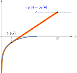
Figure 14: Party 1’s Problem: Given $G$, choosing $g=b_{1}(G)$.

Under this novel stopping rule, Party 1 (resp., Party 2) decides when to stop providing information when $p_{t}\leq 1/2$ (resp., $p_{t}>1/2$). Focusing on PSMPE, Party 1’s (resp., Party 2’s) strategy can be represented by a lower bound $g\leq 1/2$ (an upper bound $G>1/2$) at which it stops. According to the equilibrium characterization by concavification, given $G$, Party 1 chooses $g\leq 1/2$ to maximize $\frac{G-1/2}{G-g}\cdot[0-\phi_{1}(g)]+\frac{1/2-g}{G-g}\cdot 1$, where the best response is denoted by $b_{1}(G)$; given $g$, Party 2 chooses $G>1/2$ to maximize $\frac{G-1/2}{G-g}\cdot 1+\frac{1/2-g}{G-g}\cdot[0-\phi_{2}(G)]$, where the best response is denoted by $B_{2}(g)$. See Figure 14 for a graphical illustration. When $c_{i}>0$, there exists a unique solution $(g^{*},G^{*})$ such that $g^{*}=b_{1}(G^{*})$ and $G^{*}=B_{2}(g^{*})$.

The solution $(g^{*},G^{*})$ corresponds to the unique equilibrium in the baseline model of Gul and Pesendorfer (2012). Parties’ actions are strategic substitutes: Both $b_{1}$ and $B_{2}$ are increasing functions. As a result, decreasing one party’s cost makes that party provide more information and its opponent provide less.

6 Concluding Remarks

This paper studies collective dynamic information acquisition. I develop a methodology to characterize equilibrium outcomes using an ex ante perspective on posterior distributions and concavification. Players’ stopping strategies are transformed into posterior distributions and their interactions are transformed into majorization constraints. I apply my approach to different economic problems and show how it can be expanded to accommodate richer situations. Given its generality and simplicity, I believe this framework will be useful for studying other interesting problems.

To conclude, I discuss some possible extensions of the current framework.

Many States

In the baseline framework, the state is assumed to be binary. This assumption is critical for the equivalence results in Theorem 1 and equilibrium characterizations in Theorem 2. First, when $|\Theta|>2$, pure Markov strategies can no longer simply be represented by sampling regions. More importantly, when $|\Theta|>3$, not all distributions of posterior beliefs can be the result of some stopping time $\tau$, simply because multidimensional Brownian motions (or continuous Markov martingales in general) cannot hit every point in $\mathbb{R}^{n}$ almost surely when $n>2$. Rost (1971) provides a necessary and sufficient condition for feasible posterior distributions, but this condition is hard to verify. Denote the set of feasible posterior distributions by $\mathcal{G}$. Then player $i$ can only choose among some subset of $\mathcal{G}\cap\{F\mathrel{\mathop{\mathchar 58\relax}}F$ is an MPC/MPS of $F_{-i}\}$. As a result, concavification arguments analog to Theorem 2 can only provide sufficient conditions for equilibria in the dynamic games.

What Information to Acquire and How to Acquire

In the baseline framework the belief process is assumed to be exogenous, which rules out players’ control over what information to acquire and how to acquire. This framework can be enriched to allow for players’ information choice, as long as the belief process still satisfies Assumption 1 and players use Markov strategies. To illustrate, I present an example in which players can choose the level of experimentation, i.e., the precision of signals (cf. Moscarini and Smith, 2001). Assume that the dynamic of the belief process is given by $\mathrm{d}p_{t}=p_{t}(1-p_{t})\frac{2}{\sigma_{t}}\mathrm{d}B_{t}$ as in Example 1, where $(B_{t})_{t\geq 0}$ is a Brownian motion and $1/\sigma_{t}^{2}$ is the accuracy of signals. At each moment, players can exert effort to improve the accuracy $1/\sigma_{t}^{2}$ via $\sigma_{t}^{2}\equiv\Sigma(e_{1,t},e_{2,t})$ (e.g., by conducting more experiments or by presenting evidence with clearer explanations) with flow costs $K_{i}(e_{i,t})$. If we focus on Markov strategies, then $e_{i,t}=e_{i}(p_{t})$. It can be shown that the equilibrium choice of $e_{i}(\cdot)$ is independent of stopping decisions. Let $(e_{1}^{*}(\cdot),e_{2}^{*}(\cdot))$ denote the pair of equilibrium effort strategies. Then the problem between players reverts back to a stopping problem in the baseline framework with flow costs $c_{i}(p)+K_{i}(e_{i}^{*}(p))$.

Appendix A Proofs in the Baseline Framework

A.1 Ex Ante Reformulation of the Game

Proof of Lemma 1

Proof.

This is the classical Skorokhod embedding problem that asks whether there exist stopping times that embed a given distribution into a stochastic process. Obłój (2004) provides an excellent survey on this topic. According to Proposition 5.1 in Obłój (2004), for any continuous martingale $(M_{t})_{t\geq 0}$ with $M_{0}=0$ a.s. and $\langle M\rangle_{\infty}=\infty$ a.s. and any centered probability measure $\mu$ on $\mathbb{R}$, there always exists a stopping time $\tau$ in the natural filtration of $(M_{t})$ such that $M_{\tau}\sim\mu$. One proof of this result is based on the work of Chacon and Walsh (1976) which utilized potential theory. To be self-contained, I sketch the simplified proof summarized by Obłój (2004) in its Section 3.8 for later reference to some intermediate constructions.

The potential of a centered probability measure $\mu$ on $\mathbb{R}$ is defined as $U\mu(x)=-\int_{\mathbb{R}}|x-y|\mathrm{d}\mu(y)$; note that $U\mu$ is concave. For a sequence of measures $(\mu_{n})$, if $U\mu_{n}(x)\to U\mu(x)$, then $\mu_{n}\Rightarrow\mu$ (weak convergence). Therefore, in order to embed $\mu$, I can instead find a sequence of measures $\mu_{n}$ and stopping times $\tau_{n}$ such that $U\mu_{n}\to U\mu$ and $M_{\tau_{n}}\sim\mu_{n}$. If $\tau_{n}$ converges to some stopping time $\tau$ a.s., then we have $M_{\tau}\sim\mu$. Hence, it suffices to find such sequences $(\mu_{n})$ and $(\tau_{n})$.

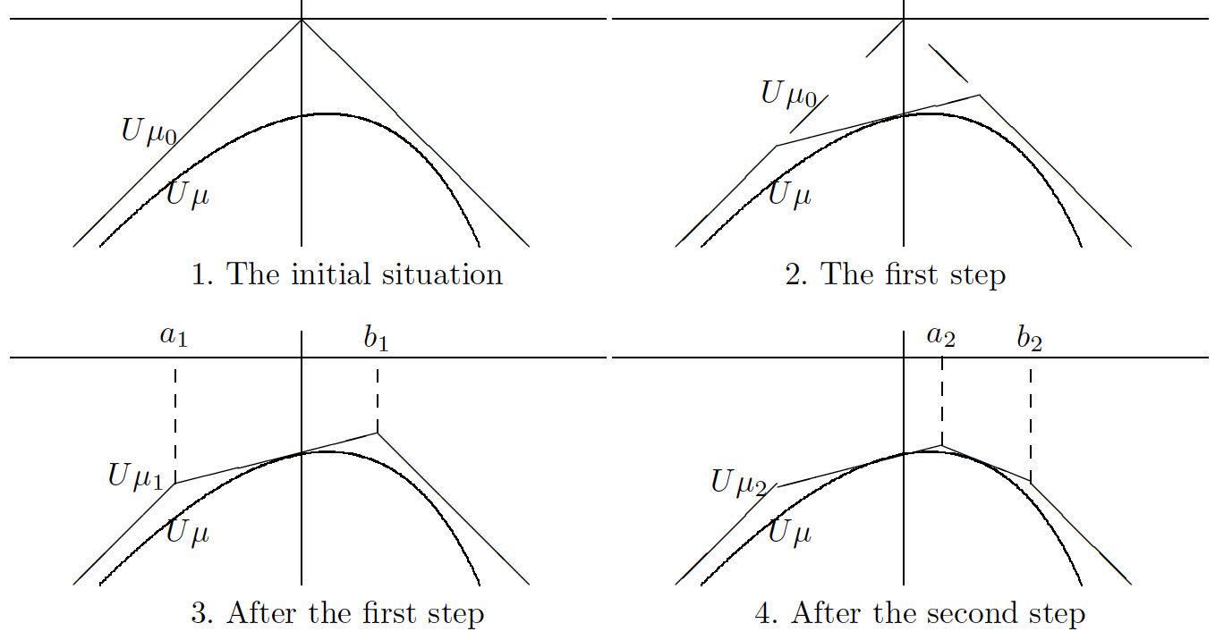
Figure 15: Illustration of the Proof. Credit to: Obłój (2004), p. 348.

See Figure 15. Write $\mu_{0}=\delta_{0}$ where $\delta_{x}$ denotes the degenerate measure at $x$. Choose a point between the graphs of $U\mu_{0}$ ($U\mu_{0}(x)=-|x|$) and $U\mu$, and draw a line $l_{1}$ through this point that stays above $U\mu$, which is possible since $U\mu$ is concave. This line cuts the potential $U\mu_{0}$ in two points $a_{1}<0<b_{1}$. Consider the new potential $U\mu_{1}$ which is given by $U\mu_{0}$ on $(-\infty,a_{1}]\cup[b_{1},\infty)$ and linear on $[a_{1},b_{1}]$. Choose a point between $U\mu_{1}$ and $U\mu$, and draw a line $l_{2}$ through this point that stays above $U\mu$ and cuts $U\mu_{1}$ in two points $a_{2}$ and $b_{2}$ such that either $a_{2}<a_{1}<b_{2}$ or $a_{2}<b_{1}<b_{2}$. Iterate this procedure. The choice of lines used to produce potentials $U\mu_{n}$ is not important. We can indeed choose lines in such a way that $U\mu_{n}\to U\mu$, because $U\mu$ is a concave function that can be represented as the infimum of a countable number of affine functions. The last step is to find the corresponding stopping times $\tau_{n}$ and the limit. Let us consider first escape times $\tau_{a,b}=\inf\{t\geq 0\mathrel{\mathop{\mathchar 58\relax}}M_{t}\in(a,b)^{c}\}$ for $a<0<b$. The assumption that $(M_{t})$ is a continuous martingale with $\langle M\rangle_{\infty}=\infty$ a.s. guarantees that the distribution of $M_{\tau_{a,b}}$ is simply $\mu_{\tau_{a,b}}=\frac{b}{b-a}\delta_{a}+\frac{-a}{b-a}\delta_{b}$. Therefore, one can check that $U\mu_{\tau_{a,b}}$ is piecewise linear. Let $\tau_{1}=\tau_{a_{1},b_{1}}$, then $M_{\tau_{1}}\sim\mu_{1}$. Let $\theta_{t}$ denote the standard shift operator and define $\tau_{2}=\tau_{1}+\tau_{a_{2},b_{2}}\circ\theta_{\tau_{1}},\dots,\tau_{n}=\tau_{n-1}+\tau_{a_{n},b_{n}}\circ\theta_{\tau_{n-1}},\dots$ and $\tau=\lim_{n\to\infty}\tau_{n}$. One can check that the limit is finite almost surely. As a result, one can embed $\mu$ via $\tau$.

Notice that in this proof the condition that $(M_{t})$ is a continuous martingale and $\langle M\rangle_{\infty}=\infty$ a.s. is only required to make sure $U\mu_{\tau_{a,b}}$ to be piecewise linear (linear on $[a,b]$) for $a<0<b$. In this regard, actually we only need $\mathbb{P}(M_{\tau_{a,b}}=a)=\frac{b}{b-a}=1-\mathbb{P}(M_{\tau_{a,b}}=b)$. When it comes to our case, to apply Proposition 5.1 in Obłój (2004), it suffices to show that $\mathbb{P}(p_{\tau_{a,b}}=a)=\frac{b-p_{0}}{b-a}$ for any $0\leq a<p_{0}<b\leq 1$. As $(p_{t})_{t\geq 0}$ is a continuous martingale and $p_{\infty}\in\{0,1\}$, $\tau_{a,b}\leq\infty$ a.s. and $p_{\tau_{a,b}}$ can only take values at $a$ or $b$. Since $(p_{\tau_{a,b}\wedge t})_{t\geq 0}$ is bounded, by Martingale Convergence Theorem, $p_{0}=\mathbb{E}[p_{\tau_{a,b}}]=\mathbb{P}(p_{\tau_{a,b}}=a)\cdot a+(1-\mathbb{P}(p_{\tau_{a,b}}=a))\cdot b$, which gives $\mathbb{P}(p_{\tau_{a,b}}=a)=\frac{b-p_{0}}{b-a}$. ∎

Proof of Lemma 2

Proof.

For the first part, since $(p_{t})$ is a martingale and $\mathcal{F}_{\rho}\subseteq\mathcal{F}_{\tau}$, by Jensen’s inequality, $\mathbb{E}[(p-p_{\tau})^{+}|\mathcal{F}_{\rho}]\geq(p-\mathbb{E}[p_{\tau}|\mathcal{F}_{\rho}])^{+}=(p-p_{\rho})^{+}$. Therefore, $\mathbb{E}[(p-p_{\tau})^{+}]=\mathbb{E}[\mathbb{E}[(p-p_{\tau})^{+}|\mathcal{F}_{\rho}]]\geq\mathbb{E}[(p-p_{\rho})^{+}]$ for any $p\in[0,1]$. This is equivalent to $\int_{0}^{p}F_{\tau}(x)dx\geq\int_{0}^{p}F_{\rho}(x)dx$ for any $p\in[0,1]$. As a result, $F_{\tau}$ is a mean-preserving spread of $F_{\rho}$.

For the second part, since $F$ is a mean-preserving spread of $F_{\rho}$, $U\mu_{F}(x)=-\int_{\mathbb{R}}|x-y|\mathrm{d}F(y)\leq-\int_{\mathbb{R}}|x-y|\mathrm{d}F_{\rho}(y)=U\mu_{F_{\rho}}(x)$. Now construct another stochastic process $(\tilde{p}_{t})$ with $\tilde{p}_{0}\sim F_{\rho}$ and $\tilde{p}_{t}=p_{t}(\tilde{p}_{0})$ for any realization of $\tilde{p}_{0}$, then according to Proposition 5.2 in Obłój (2004), there exists a stopping time $\tau^{\prime}$ such that $\tilde{p}_{\tau^{\prime}}\sim F$. Let $\tau=\rho+\tau^{\prime}\circ\theta_{\rho}$. It is easy to verify that $\tau$ is also a stopping time and $p_{\tau}\sim F$, i.e., $F_{\tau}=F$. ∎

Proof of Lemma 3

Proof.

The first part follows from Lemma 2. For the second part, according to Lemma 1, there exists a stopping time $\tau$ such that $F_{\tau}=F$. Let $\rho=\tau+\tau^{\prime}\circ\theta_{\tau}$ where $\tau^{\prime}$ is a stopping time such that $\tilde{p}_{\tau^{\prime}}\sim F$ with $\tilde{p}_{0}\sim F_{\rho}$; refer to the second part in the proof of Lemma 2. ∎

Proof of Lemma 4

Proof.

Let $\rho=\inf\{t\geq 0\mathrel{\mathop{\mathchar 58\relax}}p_{t}\in(\underline{p},\overline{p})^{c}\}$ for some $0\leq\underline{p}\leq p_{0}\leq\overline{p}\leq 1$. On the one hand, by Lemma 3, $\mathcal{E}(\rho)\subseteq\{F\mathrel{\mathop{\mathchar 58\relax}}F$ is an MPC of $F_{\rho}\}$. On the other hand, for any $F$ such that $F$ is an MPC of $F_{\rho}$, notice that the the Chacon and Walsh solution $\tau$ described in the proof of Lemma 1 is indeed such that $F_{\tau}=F$ and $\tau\leq\rho$. Recall that the sequence of $a_{n}$ and $b_{n}$ is constructed by some lines above $U\mu_{F}$. As $F$ is an MPC of $F_{\rho}$, we have $U\mu_{F_{\rho}}\leq U\mu_{F}$, so those lines are also above $U\mu_{F_{\rho}}$ and $a_{n},b_{n}\in[\underline{p},\overline{p}]$. Therefore, by construction, $\tau_{n}\leq\rho$ for all $n$. As $\tau_{n}\to\tau$ a.s., $\tau\leq\rho$ a.s. too. ∎

Proof of Lemma 5

Proof.

First, I need to show $f$ in Equation 1 is well-defined. Then the proof closely follows that of Proposition 2 in Morris and Strack (2019).

By Condition (iv) in Assumption 1, $\mathrm{d}\langle p\rangle_{s}/\mathrm{d}s$ is well-defined, i.e.,

$$\frac{\mathrm{d}\langle p\rangle_{s}}{\mathrm{d}s}=\lim_{h\to 0}\frac{\langle p\rangle_{s+h}-\langle p\rangle_{s}}{h}=\lim_{h\to 0}\frac{\langle p\rangle_{s}-\langle p\rangle_{s-h}}{h}\quad a.s.$$

Notice that $\mathrm{d}\langle p\rangle_{s}/\mathrm{d}s$ is locally integrable given Condition (iv): For any $t^{\prime}>t\geq 0$, by Tonelli’s theorem,

$$\int_{[t,t^{\prime}]}\mathbb{E}\left[\left|\mathrm{d}\langle p\rangle_{s}/\mathrm{d}s\right|\right]\mathrm{d}s=\mathbb{E}[\langle p\rangle_{t^{\prime}}-\langle p\rangle_{t}]\leq\mathbb{E}[\langle p\rangle_{t^{\prime}}]<\infty.$$

Therefore, I can interchange differentiation and expectation as follows:

$$\frac{\mathrm{d}\langle p\rangle_{s}}{\mathrm{d}s}=\lim_{h\to 0}\frac{\langle p\rangle_{s}-\langle p\rangle_{s-h}}{h}=\lim_{h\to 0}\mathbb{E}\left[\frac{\langle p\rangle_{s}-\langle p\rangle_{s-h}}{h}|\mathcal{F}_{s}\right]=\mathbb{E}\left[\lim_{h\to 0}\frac{\langle p\rangle_{s}-\langle p\rangle_{s-h}}{h}|\mathcal{F}_{s}\right]$$

$$=\mathbb{E}\left[\lim_{h\to 0}\frac{\langle p\rangle_{s+h}-\langle p\rangle_{s}}{h}|\mathcal{F}_{s}\right]=\lim_{h\to 0}\mathbb{E}\left[\frac{\langle p\rangle_{s+h}-\langle p\rangle_{s}}{h}|\mathcal{F}_{s}\right]=\lim_{h\to 0}\mathbb{E}\left[\frac{\langle p\rangle_{s+h}-\langle p\rangle_{s}}{h}|p_{s}\right].$$

The last equality is because $(p_{t})$ is Markov. In sum, $\mathrm{d}\langle p\rangle_{s}/\mathrm{d}s$ is $\sigma(p_{s})$-measurable, i.e., there exits a function $f$ such that $\mathrm{d}\langle p\rangle_{s}/\mathrm{d}s=f(p_{s})$ a.s.. By Condition (iv) in Assumption 1, $f(p_{s})$ must be strictly positive a.s..

Let $\tau$ be an arbitrary a.s. finite stopping time. Applying Ito’s lemma, I obtain

$$\phi_{i}(p_{t})=\phi_{i}(p_{0})+\int_{0}^{t}\phi_{i}^{\prime}(p_{s})\mathrm{d}p_{s}+\int_{0}^{t}\frac{1}{2}\phi_{i}^{\prime\prime}(p_{s})\mathrm{d}\langle p\rangle_{s}.$$ (4)

By Equation 1, $\phi_{i}^{\prime\prime}(p_{s})=2c_{i}(p_{s})/f(p_{s})$. As a result, I can rewrite Equation 4 as

$$\phi_{i}(p_{t})=\phi_{i}(p_{0})+\int_{0}^{t}\phi_{i}^{\prime}(p_{s})\mathrm{d}p_{s}+\int_{0}^{t}c_{i}(p_{s})\mathrm{d}s.$$

Define

$$r_{n}\mathrel{\mathop{\mathchar 58\relax}}=n\wedge\inf\left\{t\geq 0\mathrel{\mathop{\mathchar 58\relax}}\int_{0}^{t}\left|\phi_{i}^{\prime}(p_{s})\right|^{2}\mathrm{d}\langle p\rangle_{s}\geq n\right\}.$$

Due to the definition of $r_{n}$, the stochastic integral $\int_{0}^{t\wedge r_{n}}\phi_{i}^{\prime}(p_{s})\mathrm{d}p_{s}$ is an integrable martingale, given that $(p_{t})$ is a continuous martingale. Since $\tau\wedge r_{n}$ is finite, by the optional stopping theorem, the expectation of this integral at $\tau\wedge r_{n}$ is equal to zero. Therefore,

$$\mathbb{E}[\phi_{i}(p_{\tau\wedge r_{n}})]-\phi_{i}(p_{0})=\mathbb{E}\left[\int_{0}^{\tau\wedge r_{n}}\frac{1}{2}\phi_{i}^{\prime\prime}(p_{s})\mathrm{d}\langle p\rangle_{s}\right]=\mathbb{E}\left[\int_{0}^{\tau\wedge r_{n}}c_{i}(p_{s})\mathrm{d}s\right],$$

Notice that $r_{n}\to\infty$ and thus $\tau\wedge r_{n}\to\tau$ as $n\to\infty$. It remains to show that the equality holds in the limit, the argument for which is exactly the same as in the proof of Proposition 2 in Morris and Strack (2019). ∎

Proof of Theorem 1

Proof.

Notice that part (ii) implies the statement on PSMPE in Theorem 1 for unanimous stopping. Therefore, I only prove this statement on PSMPE for unilateral stopping, deferring the proof for unanimous stopping to the general case in part (ii). Let $\tau_{i}$ denote player $i$’s stopping time. Player $i$’s expected payoff of using $\tau_{i}$ is

$$\mathbb{E}\left[u_{i}(p_{\tau_{i}\wedge\tau_{-i}})\mathbbm{1}_{\tau_{i}\wedge\tau_{-i}<\infty}-\int_{0}^{\tau_{i}\wedge\tau_{-i}}c_{i}(p_{s})\mathrm{d}s\right]=\int_{0}^{1}[u_{i}(p)-\phi_{i}(p)]\mathrm{d}F_{\tau_{i}\wedge\tau_{-i}}(p),$$

by Lemma 5 since $\tau_{i}\wedge\tau_{-i}\leq\tau_{i}<\infty$ by optimality. When $\tau_{-i}$ is a Markov stopping time, $\tau_{i}$ is a best response of player $i$ to $\tau_{-i}$ if and only if $F_{\tau_{i}\wedge\tau_{-i}}$ is her best choice among all MPCs of $F_{\tau_{-i}}$ according to Lemma 4. Therefore, $(\tau_{1},\tau_{2})$ is a PSMPE under unilateral stopping (implying that $\tau_{i}$ is a Markov stopping time and thus $F_{\tau_{i}}$ a binary policy) if and only if $(F_{\tau_{1}},F_{\tau_{2}})$ is a binary policy solution to Problem (3) since $F_{\tau_{i}\wedge\tau_{-i}}=F_{\tau_{i}}\wedge F_{\tau_{-i}}$ for binary policies $\tau_{i},\tau_{-i}$.

More generally, for part (i), suppose that $F_{i}\wedge F_{-i}$ is a best response to $F_{-i}$ in Problem (3). By Lemma 3 there exist $\tau_{1}$ and $\tau_{2}$ such that $F_{\tau_{1}\wedge\tau_{2}}=F_{1}\wedge F_{2},F_{\tau_{1}}=F_{1}$ and $F_{\tau_{2}}=F_{2}$. Moreover, $F_{\tau_{i}\wedge\tau_{-i}}$ is also optimal in $\mathcal{E}(\tau_{-i})=\{F\mathrel{\mathop{\mathchar 58\relax}}\exists\tau\leq\tau_{-i}$ a.s. such that $F=F_{\tau}\}$, which is a subset of $\{F\mathrel{\mathop{\mathchar 58\relax}}F$ is an MPC of $F_{\tau_{-i}}\}$. As a result, $\tau_{i}$ is a best response to $\tau_{-i}$ in Problem (2.2.2). In conclusion, if $(F_{1},F_{2})$ is a solution to Problem (3), then there exists an NE under unilateral stopping characterized by $(\tau_{1},\tau_{2})$ such that $F_{\tau_{i}}=F_{i}$.

Finally for part (ii), notice that player $i$’s expected payoff of using $\tau_{i}$ under unanimous stopping is

$$\mathbb{E}\left[u_{i}(p_{\tau_{i}\vee\tau_{-i}})\mathbbm{1}_{\tau_{i}\vee\tau_{-i}<\infty}-\int_{0}^{\tau_{i}\vee\tau_{-i}}c_{i}(p_{s})\mathrm{d}s\right]=\int_{0}^{1}[u_{i}(p)-\phi_{i}(p)]\mathrm{d}F_{\tau_{i}\vee\tau_{-i}}(p),$$

by Lemma 5 since $\tau_{i}\vee\tau_{-i}<\infty$ by optimality. According to Lemma 2, $\tau_{i}$ is a best response of player $i$ to $\tau_{-i}$ if and only if $F_{\tau_{i}\vee\tau_{-i}}$ is her best choice among all MPSs of $F_{\tau_{-i}}$. This proves part (ii) in the general case. ∎

A.2 Equilibrium Analysis

Proof of Theorem 2

Proof.

Unilateral Stopping: For the “if” part, let $F_{\underline{p},\overline{p}}$ denote the binary policy with support $\overline{p}$ and $\underline{p}$ and $\mathbb{E}_{F_{\underline{p},\overline{p}}}[p]=p_{0}$. By definition, $V_{i}^{Uni}(p_{0};\underline{p},\overline{p})\geq\int_{0}^{1}[u_{i}(p)-\phi_{i}(p)]\mathrm{d}F(p)$ for any $F$ that is an MPC of $F_{\underline{p},\overline{p}}$. Since $\int_{0}^{1}[u_{i}(p)-\phi_{i}(p)]\mathrm{d}F_{\underline{p},\overline{p}}(p)=\frac{\overline{p}-p_{0}}{\overline{p}-\underline{p}}[u_{i}(\underline{p})-\phi_{i}(\underline{p})]+\frac{p_{0}-\underline{p}}{\overline{p}-\underline{p}}[u_{i}(\overline{p})-\phi_{i}(\overline{p})]=V_{i}^{Uni}(p_{0};\underline{p},\overline{p})$, $F_{\underline{p},\overline{p}}$ is optimal among all MPCs of $F_{\underline{p},\overline{p}}$ for player $i$. Therefore, $(F_{\underline{p},\overline{p}},F_{\underline{p},\overline{p}})$ a solution to Problem (3).

For the “only if” part, by definition, $\frac{\overline{p}-p_{0}}{\overline{p}-\underline{p}}[u_{i}(\underline{p})-\phi_{i}(\underline{p})]+\frac{p_{0}-\underline{p}}{\overline{p}-\underline{p}}[u_{i}(\overline{p})-\phi_{i}(\overline{p})]\leq V_{i}^{Uni}(p_{0};\underline{p},\overline{p})$ for $i=1,2$. Suppose that one of the inequalities is strict, say $\frac{\overline{p}-p_{0}}{\overline{p}-\underline{p}}[u_{1}(\underline{p})-\phi_{1}(\underline{p})]+\frac{p_{0}-\underline{p}}{\overline{p}-\underline{p}}[u_{1}(\overline{p})-\phi_{1}(\overline{p})]<V_{1}^{Uni}(p_{0};\underline{p},\overline{p})$. By the definition of concave closure, for any $\epsilon>0$, there exists a distribution over $[\underline{p},\overline{p}]$ denoted by $F$ such that $\mathbb{E}_{F}[p]=p_{0}$ and $\int_{[\underline{p},\overline{p}]}[u_{1}(p)-\phi_{1}(p)]\mathrm{d}F(p)\in\left(V_{1}^{Uni}(p_{0};\underline{p},\overline{p})-\epsilon,V_{1}^{Uni}(p_{0};\underline{p},\overline{p})\right]$. Since $\epsilon>0$ is arbitrary, there exists a distribution $F$ over $[\underline{p},\overline{p}]$ such that $\mathbb{E}_{F}[p]=p_{0}$ and $\int_{[\underline{p},\overline{p}]}[u_{1}(p)-\phi_{1}(p)]\mathrm{d}F(p)>\frac{\overline{p}-p_{0}}{\overline{p}-\underline{p}}[u_{1}(\underline{p})-\phi_{1}(\underline{p})]+\frac{p_{0}-\underline{p}}{\overline{p}-\underline{p}}[u_{1}(\overline{p})-\phi_{1}(\overline{p})]=\int_{[\underline{p},\overline{p}]}[u_{1}(p)-\phi_{1}(p)]\mathrm{d}F_{\underline{p},\overline{p}}(p)$, which implies that $F$ is strictly better than $F_{\underline{p},\overline{p}}$ for player 1. Notice that $F$ is an MPC of $F_{\underline{p},\overline{p}}$. This contradicts $F_{\underline{p},\overline{p}}$ being optimal for player 1 in Problem (3). Therefore, equalities must hold.

Unanimous Stopping: The proof is similar and omitted for brevity. ∎

Proof of Lemma 6

Proof.

Unilateral Stopping: Fix two equilibrium sampling regions $[\underline{p},\overline{p}]$ and $[\underline{p}^{\prime},\overline{p}{}^{\prime}]$. It is without loss to only consider the situation with $\underline{p}\leq\underline{p}^{\prime}\leq p_{0}\leq\overline{p}\leq\overline{p}{}^{\prime}$. Since $[\underline{p},\overline{p}]$ is an equilibrium outcome, by Theorem 2 and in particular Equation 2, we have

$$\frac{\overline{p}-p}{\overline{p}-\underline{p}}[u_{i}(\underline{p})-\phi_{i}(\underline{p})]+\frac{p-\underline{p}}{\overline{p}-\underline{p}}[u_{i}(\overline{p})-\phi_{i}(\overline{p})]=V_{i}^{Uni}\left(p;\underline{p},\overline{p}\right)\geq u_{i}(p)-\phi_{i}(p),\quad\forall p\in[\underline{p},\overline{p}].$$

Therefore, the line connecting points $(\underline{p},u_{i}(\underline{p})-\phi_{i}(\underline{p}))$ and $(\overline{p},u_{i}(\overline{p})-\phi_{i}(\overline{p}))$ is above the graph of $u_{i}-\phi_{i}$ within $[\underline{p},\overline{p}]$.

Similarly, for $[\underline{p}^{\prime},\overline{p}{}^{\prime}]$, we also have

$$\frac{\overline{p}{}^{\prime}-p}{\overline{p}{}^{\prime}-\underline{p}^{\prime}}[u_{i}(\underline{p}^{\prime})-\phi_{i}(\underline{p}^{\prime})]+\frac{p-\underline{p}^{\prime}}{\overline{p}{}^{\prime}-\underline{p}^{\prime}}[u_{i}(\overline{p}{}^{\prime})-\phi_{i}(\overline{p}{}^{\prime})]=V_{i}^{Uni}\left(p;\underline{p}^{\prime},\overline{p}{}^{\prime}\right)\geq u_{i}(p)-\phi_{i}(p),\text{ }\forall p\in[\underline{p}^{\prime},\overline{p}{}^{\prime}],$$

i.e., the line connecting points $(\underline{p}^{\prime},u_{i}(\underline{p}^{\prime})-\phi_{i}(\underline{p}^{\prime}))$ and $(\overline{p}{}^{\prime},u_{i}(\overline{p}{}^{\prime})-\phi_{i}(\overline{p}{}^{\prime}))$ is above the graph of $u_{i}-\phi_{i}$ within $[\underline{p}^{\prime},\overline{p}{}^{\prime}]$.

By the above two inequalities and some simple algebra, we can derive

$$\frac{\overline{p}{}^{\prime}-p}{\overline{p}{}^{\prime}-\underline{p}}[u_{i}(\underline{p})-\phi_{i}(\underline{p})]+\frac{p-\underline{p}}{\overline{p}{}^{\prime}-\underline{p}}[u_{i}(\overline{p}{}^{\prime})-\phi_{i}(\overline{p}{}^{\prime})]\geq u_{i}(p)-\phi_{i}(p),\quad\forall p\in[\underline{p},\overline{p}{}^{\prime}].$$

Thus,

$$\frac{\overline{p}{}^{\prime}-p}{\overline{p}{}^{\prime}-\underline{p}}[u_{i}(\underline{p})-\phi_{i}(\underline{p})]+\frac{p-\underline{p}}{\overline{p}{}^{\prime}-\underline{p}}[u_{i}(\overline{p}{}^{\prime})-\phi_{i}(\overline{p}{}^{\prime})]=V_{i}^{Uni}\left(p;\underline{p},\overline{p}{}^{\prime}\right),\quad\forall p\in[\underline{p},\overline{p}{}^{\prime}].$$

As a result, $[\underline{p},\overline{p}{}^{\prime}]$ is also an equilibrium under unilateral stopping.

Unanimous Stopping: The proof is symmetric and omitted for brevity. ∎

Proof of Proposition 1

Proof.

Unilateral Stopping: Let $[\underline{p},\overline{p}]$ be an equilibrium sampling region under unilateral stopping. Construct two virtual players with the same terminal payoff $\lambda_{1}u_{1}+\lambda_{2}u_{2}$ and the same sampling cost $\lambda_{1}c_{1}+\lambda_{2}c_{2}$. Hence, these virtual players’ expected payoffs from a posterior distribution $F$ are exactly $\mathbb{E}_{F}[W(p;\lambda)]$. Notice that both $[\underline{p},\overline{p}]$ and the $\lambda$-efficient outcome $[\underline{p}{}_{\lambda}^{*},\overline{p}{}_{\lambda}^{*}]$ are equilibrium outcomes under unilateral stopping between these two virtual players. Therefore, by Lemma 6, $\left[\min\{\underline{p},\underline{p}{}_{\lambda}^{*}\},\max\{\overline{p},\overline{p}{}_{\lambda}^{*}\}\right]$ is also an equilibrium sampling region. By definition of equilibrium under unilateral stopping, the virtual player with an objective of $\mathbb{E}_{F}[W(p;\lambda)]$ prefers $\left[\min\{\underline{p},\underline{p}{}_{\lambda}^{*}\},\max\{\overline{p},\overline{p}{}_{\lambda}^{*}\}\right]$ to $[\underline{p}{}_{\lambda}^{*},\overline{p}{}_{\lambda}^{*}]$. Because $[\underline{p}{}_{\lambda}^{*},\overline{p}{}_{\lambda}^{*}]$ is uniquely $\lambda$-efficient, it must be $\left[\min\{\underline{p},\underline{p}{}_{\lambda}^{*}\},\max\{\overline{p},\overline{p}{}_{\lambda}^{*}\}\right]=[\underline{p}{}_{\lambda}^{*},\overline{p}{}_{\lambda}^{*}]$ and thus $[\underline{p},\overline{p}]$ is smaller than $[\underline{p}{}_{\lambda}^{*},\overline{p}{}_{\lambda}^{*}]$.

Unanimous Stopping: The proof is symmetric and omitted for brevity. ∎

Proof of Lemma 7

Proof.

Let $T^{b}$ denote the set of all equilibrium sampling regions when misalignment is $b$.

Fix an arbitrary $[\underline{p},\overline{p}]\in T^{b}$ and let $F_{\underline{p},\overline{p}}$ denote the corresponding binary policy. Since $c_{1}(\cdot)=c_{2}(\cdot)$, let $\phi(\cdot)\mathrel{\mathop{\mathchar 58\relax}}=\phi_{i}(\cdot)$. By Theorem 1, we have $\int_{0}^{1}[u_{i}(p;b)-\phi(p)]\mathrm{d}F_{\underline{p},\overline{p}}\geq\int_{0}^{1}[u_{i}(p;b)-\phi(p)]\mathrm{d}F$ for any $F$ that is an MPC (resp., MPS) of $F_{\underline{p},\overline{p}}$. Since $u_{1}=f+bg$ and $u_{2}=f-bg$, for any $F$ that is an MPC (resp., MPS) of $F_{\underline{p},\overline{p}}$ and for any $b^{\prime}\in[0,b)$,

$$\int_{0}^{1}\left[f(p)-\phi(p)\right]\mathrm{d}\left(F_{\underline{p},\overline{p}}-F\right)\geq b\left|\int_{0}^{1}g(p)\mathrm{d}\left(F_{\underline{p},\overline{p}}-F\right)\right|\geq b^{\prime}\left|\int_{0}^{1}g(p)\mathrm{d}\left(F_{\underline{p},\overline{p}}-F\right)\right|.$$

It thus implies that $\int_{0}^{1}[u_{i}(p;b^{\prime})-\phi(p)]\mathrm{d}F_{\underline{p},\overline{p}}\geq\int_{0}^{1}[u_{i}(p;b^{\prime})-\phi(p)]\mathrm{d}F$ for any $F$ that is an MPC (resp., MPS) of $F_{\underline{p},\overline{p}}$. As a result, $[\underline{p},\overline{p}]\in T^{b^{\prime}}$. Hence, $T^{b}\subset T^{b^{\prime}}$ for any $b>b^{\prime}\geq 0$. ∎

Proof of Proposition 2

Proof.

Directly follows from Lemmas 6 and 7. ∎

Appendix B Proofs in the Applications

B.1 Committee Search

Proof of Proposition 3

Proof.

Notice that $U_{i}(\underline{p}^{q},\overline{p};p_{0})$ is strict concave in $\overline{p}$ over $[t_{l},1]$ and has strict decreasing differences in $(\overline{p};v_{i})$. Therefore, $\overline{B}_{i}(\underline{p}^{q})$ is a singleton and decreasing in $v_{i}$. Similarly, since $U_{i}(\underline{p},\overline{p}{}^{q};p_{0})$ is strict concave in $\underline{p}$ over $[0,t_{l})$ and has strict decreasing differences in $(\underline{p};v_{i})$, $\underline{B}{}_{i}(\overline{p}^{q})$ is a singleton and decreasing in $v_{i}$. As a result, $\overline{B}_{i}\leq\overline{B}_{j}$ and $\underline{B}{}_{i}\leq\underline{B}{}_{j}$ for any $i\leq j$.

Lemma 9.

Suppose that players are homogeneous in sampling costs. A sampling region $[\underline{p},\overline{p}]$ is an equilibrium outcome with one-sided best responses (OSBR) under the $q$-collective stopping rule if and only if $\overline{p}=\overline{B}_{2m-q}(\underline{p})$ and $\underline{p}=\underline{B}{}_{q}(\overline{p})$.

Proof.

The “only if” part is simply by the requirement of one-sided best responses.

Consider the “if” part. Let $\overline{p}_{i}=\overline{B}_{i}(\underline{p})$ and $\underline{p}{}_{i}=\underline{B}{}_{i}(\overline{p})$, so $\underline{p}^{q}=\underline{B}{}_{q}(\overline{p})=\underline{p}$, $\overline{p}^{q}=\overline{B}_{2m-q}(\underline{p})=\overline{p}$, and the requirement of one-sided best responses is automatically satisfied. It remains to check whether $\{(\underline{p}{}_{i},\overline{p}_{i})\}_{i}$ constitutes an equilibrium, i.e., whether Condition ($q$-collective) holds.

When $\boldsymbol{q\geq m}$: For player $i>q$, because $U_{i}(\underline{p}{}_{q},\overline{p};p_{0})$ is single-peaked in $\overline{p}$ over $[t_{l},1]$ and $t_{l}\leq\overline{B}_{i}(\underline{p}{}_{q})\leq\overline{B}_{2m-q}(\underline{p}{}_{q})=\overline{p}_{2m-q}$, we have $U_{i}(\underline{p}{}_{q},\overline{p}_{2m-q};p_{0})\geq U_{i}(\underline{p}{}_{q},\overline{p}{}^{\prime};p_{0})$ for any $\overline{p}{}^{\prime}\geq\overline{p}_{2m-q}$. Similarly, $U_{i}(\underline{p}{}_{q},\overline{p}_{2m-q};p_{0})\geq U_{i}(\underline{p}^{\prime},\overline{p}_{2m-q};p_{0})$ for any $\underline{p}^{\prime}\in[\underline{p}{}_{q},t_{l}\wedge p_{0})$. Notice that player $i$’s span of control is $(\underline{p}^{\prime},\overline{p}{}^{\prime})\in[\underline{p}{}_{q},\underline{p}_{q-1}]\times[\overline{p}_{2m-q},\overline{p}_{2m-q-1}]$ (where $\overline{p}_{0}\mathrel{\mathop{\mathchar 58\relax}}=1$). As discussed, for any such pair of $\underline{p}^{\prime}$ and $\overline{p}{}^{\prime}$, we have

$$\frac{\overline{p}_{2m-q}-p_{0}}{\overline{p}_{2m-q}-\underline{p}{}_{q}} [u_{i}(\underline{p}{}_{q})-\phi_{i}(\underline{p}{}_{q})]+\frac{p_{0}-\underline{p}{}_{q}}{\overline{p}_{2m-q}-\underline{p}{}_{q}}[u_{i}(\overline{p}_{2m-q})-\phi_{i}(\overline{p}_{2m-q})]=U_{i}\left(\underline{p}{}_{q},\overline{p}_{2m-q};p_{0}\right)$$

$$\geq U_{i}\left(\underline{p}{}_{q},\overline{p}{}^{\prime};p_{0}\right)=\frac{\overline{p}{}^{\prime}-p_{0}}{\overline{p}{}^{\prime}-\underline{p}{}_{q}}[u_{i}(\underline{p}{}_{q})-\phi_{i}(\underline{p}{}_{q})]+\frac{p_{0}-\underline{p}{}_{q}}{\overline{p}{}^{\prime}-\underline{p}{}_{q}}[u_{i}(\overline{p}{}^{\prime})-\phi_{i}(\overline{p}{}^{\prime})],$$

$$\frac{\overline{p}_{2m-q}-p_{0}}{\overline{p}_{2m-q}-\underline{p}{}_{q}}[u_{i}(\underline{p}{}_{q})-\phi_{i}(\underline{p}{}_{q})]+\frac{p_{0}-\underline{p}{}_{q}}{\overline{p}_{2m-q}-\underline{p}{}_{q}}[u_{i}(\overline{p}_{2m-q})-\phi_{i}(\overline{p}_{2m-q})]=U_{i}\left(\underline{p}{}_{q},\overline{p}_{2m-q};p_{0}\right)$$

$$\geq U_{i}\left(\underline{p}^{\prime},\overline{p}_{2m-q};p_{0}\right)=\frac{\overline{p}_{2m-q}-p_{0}}{\overline{p}_{2m-q}-\underline{p}^{\prime}}[u_{i}(\underline{p}^{\prime})-\phi_{i}(\underline{p}^{\prime})]+\frac{p_{0}-\underline{p}^{\prime}}{\overline{p}_{2m-q}-\underline{p}^{\prime}}[u_{i}(\overline{p}_{2m-q})-\phi_{i}(\overline{p}_{2m-q})].$$

These two inequalities imply that for any $(\underline{p}^{\prime},\overline{p}{}^{\prime})\in[\underline{p}{}_{q},\underline{p}_{q-1}]\times[\overline{p}_{2m-q},\overline{p}_{2m-q-1}]$,

$$U_{i}\left(\underline{p}{}_{q},\overline{p}_{2m-q};p_{0}\right)=\frac{\overline{p}_{2m-q}-p_{0}}{\overline{p}_{2m-q}-\underline{p}{}_{q}}[u_{i}(\underline{p}{}_{q})-\phi_{i}(\underline{p}{}_{q})]+\frac{p_{0}-\underline{p}{}_{q}}{\overline{p}_{2m-q}-\underline{p}{}_{q}}[u_{i}(\overline{p}_{2m-q})-\phi_{i}(\overline{p}_{2m-q})]$$

$$\geq\frac{\overline{p}{}^{\prime}-p_{0}}{\overline{p}{}^{\prime}-\underline{p}^{\prime}}[u_{i}(\underline{p}^{\prime})-\phi_{i}(\underline{p}^{\prime})]+\frac{p_{0}-\underline{p}^{\prime}}{\overline{p}{}^{\prime}-\underline{p}^{\prime}}[u_{i}(\overline{p}{}^{\prime})-\phi_{i}(\overline{p}{}^{\prime})]=U_{i}\left(\underline{p}^{\prime},\overline{p}{}^{\prime};p_{0}\right).$$

The first two inequalities imply the line connecting points $(\underline{p}{}_{q},(u_{i}-\phi_{i})(\underline{p}{}_{q}))$ and $(\overline{p}_{2m-q},(u_{i}-\phi_{i})(\overline{p}_{2m-q}))$ is above the line connecting $(\underline{p}{}_{q},(u_{i}-\phi_{i})(\underline{p}{}_{q}))$ and $(\overline{p}{}^{\prime},(u_{i}-\phi_{i})(\overline{p}{}^{\prime}))$ over $[\underline{p}{}_{q},\overline{p}{}^{\prime}]$, and is also above the one connecting $(\underline{p}^{\prime},(u_{i}-\phi_{i})(\underline{p}^{\prime}))$ and $(\overline{p}_{2m-q},(u_{i}-\phi_{i})(\overline{p}_{2m-q}))$ over $[\underline{p}{}_{q},\overline{p}_{2m-q}]$. As a result, the line connecting $(\underline{p}{}_{q},(u_{i}-\phi_{i})(\underline{p}{}_{q}))$ and $(\overline{p}_{2m-q},(u_{i}-\phi_{i})(\overline{p}_{2m-q}))$ is above the one connecting $(\underline{p}^{\prime},(u_{i}-\phi_{i})(\underline{p}^{\prime}))$ and $(\overline{p}{}^{\prime},(u_{i}-\phi_{i})(\overline{p}{}^{\prime}))$ over $[\underline{p}^{\prime},\overline{p}{}^{\prime}]$, as indicated by the last inequality. Therefore, $U_{i}(\underline{p}{}_{q},\overline{p}_{2m-q};p_{0})\geq U_{i}(\underline{p}^{\prime},\overline{p}{}^{\prime};p_{0})$ and thus Condition ($q$-collective) holds. The analysis for player $i<2m-q$ is symmetric.

For player $i$ with $2m-q<i<q$, also by single-peakedness, $U_{i}(\underline{p}{}_{q},\overline{p}_{2m-q};p_{0})\geq U_{i}(\underline{p}{}_{q},\overline{p}{}^{\prime};p_{0})$ for any $\overline{p}{}^{\prime}\geq\overline{p}_{2m-q}$ and $U_{i}(\underline{p}{}_{q},\overline{p}_{2m-q};p_{0})\geq U_{i}(\underline{p}^{\prime},\overline{p}_{2m-q};p_{0})$ for any $\underline{p}^{\prime}\leq\underline{p}{}_{q}$. Player $i$’s span of control is $(\underline{p}^{\prime},\overline{p}{}^{\prime})\in[\underline{p}{}_{q+1},\underline{p}{}_{q}]\times[\overline{p}_{2m-q},\overline{p}_{2m-q-1}]$. For any such pair of $\underline{p}^{\prime}$ and $\overline{p}{}^{\prime}$, using the same argument, we can show that $U_{i}(\underline{p}{}_{q},\overline{p}_{2m-q};p_{0})\geq U_{i}(\underline{p}^{\prime},\overline{p}{}^{\prime};p_{0})$ and thus Condition ($q$-collective) holds.

For player $2m-q$, by definition, $U_{i}(\underline{p}{}_{q},\overline{p}_{2m-q};p_{0})\geq U_{i}(\underline{p}{}_{q},\overline{p}{}^{\prime};p_{0})$ for any $\overline{p}{}^{\prime}\geq t_{l}\vee p_{0}$, and by single-peakedness, $U_{i}(\underline{p}{}_{q},\overline{p}_{2m-q};p_{0})\geq U_{i}(\underline{p}^{\prime},\overline{p}_{2m-q};p_{0})$ for any $\underline{p}^{\prime}\leq\underline{p}{}_{q}$. Player $i$’s span of control is $(\underline{p}^{\prime},\overline{p}{}^{\prime})\in[\underline{p}{}_{q+1},\underline{p}{}_{q}]\times[\overline{p}_{2m-q+1},\overline{p}_{2m-q-1}]$. By the same argument, $U_{i}(\underline{p}{}_{q},\overline{p}_{2m-q};p_{0})\geq U_{i}(\underline{p}^{\prime},\overline{p}{}^{\prime};p_{0})$ for any such $\underline{p}^{\prime}$ and $\overline{p}{}^{\prime}$, so Condition ($q$-collective) holds. Symmetric for player $q$.

In conclusion, Condition ($q$-collective) holds for all players. As a result, when $q\geq m$, a sampling region $[\underline{p},\overline{p}]$ is an equilibrium outcome with one-sided best responses under the $q$-collective stopping rule if and only if $\overline{p}=\overline{B}_{2m-q}(\underline{p})$ and $\underline{p}=\underline{B}{}_{q}(\overline{p})$.

When $\boldsymbol{q\leq m}$: Instead of $q\geq 2m-q$, now $2m-q\leq q$. When $q>1$, the analysis is symmetric to the case with $q\geq m$, according which it can be shown that Condition ($q$-collective) holds for all players. However, when $q=1$, things are a bit more subtle because now player $i$’s span of control is $(\underline{p}^{\prime},\overline{p}{}^{\prime})\in[\underline{p}{}_{1},p_{0}]\times[p_{0},\overline{p}_{2m-1}]$ for any $1<i<2m-1$—player $i$ can choose a lower bound above $t_{l}$ or an upper bound below $t_{l}$, but the best responses are only defined on one side of $t_{l}$. Without loss consider the case when $p_{0}<t_{l}$.

For player $i$ such that $1<i<2m-1$, following the previous logic based on the single-peakedness of $U_{i}$, we know $U_{i}(\underline{p}{}_{1},\overline{p}_{2m-1};p_{0})\geq U_{i}(\underline{p}^{\prime},\overline{p}{}^{\prime};p_{0})$ for any $\underline{p}^{\prime}\in[\underline{p}{}_{1},p_{0}]$ and $\overline{p}{}^{\prime}\in[t_{l},\overline{p}_{2m-1}]$. It remains to check the deviations in terms of $(\underline{p}^{\prime},\overline{p}{}^{\prime})\in[\underline{p}{}_{1},p_{0}]\times[p_{0},t_{l})$. Since $u_{i}-\phi_{i}$ is concave on the left of $t_{l}$, among these deviations, $\underline{p}^{\prime}=\overline{p}{}^{\prime}=p_{0}$ is the most profitable and $U_{i}(p_{0},p_{0};p_{0})=u_{i}(p_{0})-\phi_{i}(p_{0})$. Notice that $U_{i}(\underline{p}{}_{1},\overline{p}_{2m-1};p_{0})\geq U_{i}(p_{0},\overline{p}_{2m-1};p_{0})=U_{i}(p_{0},p_{0};p_{0})$. As a result, Condition ($q$-collective) holds for player $i$.

For player $2m-1$, her span of control is instead given by $(\underline{p}^{\prime},\overline{p}{}^{\prime})\in[\underline{p}{}_{1},p_{0}]\times[p_{0},\overline{p}_{2m-2}]$. All the previous arguments follow despite this difference. Similar for player $1$. Therefore, Condition ($q$-collective) holds for them too.

In conclusion, Condition ($q$-collective) holds. As a result, when $q\leq m$, a sampling region $[\underline{p},\overline{p}]$ is an equilibrium outcome with one-sided best responses under the $q$-collective stopping rule if and only if $\overline{p}=\overline{B}_{2m-q}(\underline{p})$ and $\underline{p}=\underline{B}{}_{q}(\overline{p})$. ∎

Since unanimous stopping is a special $q$-stopping rule, the statement for $q\geq m$ in Proposition 3 is immediately obtained by replacing $q$-collective stopping between $2m-1$ players with unanimous stopping between player $q$ and player $2m-q$ in Lemma 9. It is unanimous stopping between these two players because $\underline{B}{}_{q}\leq\underline{B}{}_{2m-q}$ and $\overline{B}_{q}\leq\overline{B}_{2m-q}$ when $q\geq m$.

Similarly, unilateral stopping is a special $q$-stopping rule with $q=1$. We can obtain the statement for $q\leq m$ in Proposition 3 by replacing $q$-collective stopping between $2m-1$ players with unilateral stopping between player $q$ and player $2m-q$. It is unilateral stopping between these two players because $\underline{B}{}_{q}\geq\underline{B}{}_{2m-q}$ and $\overline{B}_{q}\geq\overline{B}_{2m-q}$ when $q\leq m$. ∎

Proof of Lemma 8

Proof.

Consider $q<m$. Let $[\underline{p}{}_{\max},\overline{p}{}_{\max}]$ denote the maximum equilibrium under unilateral stopping. Suppose that $[\underline{p}{}_{\max},\overline{p}{}_{\max}]$ does not have one-sided best responses (OSBR), so either $\underline{p}{}_{\max}\neq\underline{B}{}_{q}(\overline{p}_{\max})=\mathrel{\mathop{\mathchar 58\relax}}\underline{p}$ or $\overline{p}{}_{\max}\neq\overline{B}{}_{2m-q}(\underline{p}{}_{\max})=\mathrel{\mathop{\mathchar 58\relax}}\overline{p}$. Suppose that $\underline{p}{}_{\max}\neq\underline{p}$, then it must be $\underline{p}{}_{\max}>\underline{p}$, because otherwise player $q$ has strict incentive to deviate to $[\underline{p},\overline{p}{}_{\max}]$ from $[\underline{p}{}_{\max},\overline{p}{}_{\max}]$, leading to a contradiction. Consider a new sampling region $[\underline{p},\overline{p}{}_{\max}]$. By definition of $\underline{p}=\underline{B}{}_{q}(\overline{p}_{\max})$, we have $U_{q}(\underline{p},\overline{p}{}_{\max};p_{0})\geq U_{q}(p,\overline{p}{}_{\max};p_{0})$ for all $p\in[\underline{p},\underline{p}{}_{\max}]$. It implies

$$U_{q}\left(\underline{p},\overline{p}{}_{\max};p_{0}\right)\geq U_{q}\left(\underline{p}{}_{\max},\overline{p}{}_{\max};p_{0}\right)=V_{q}^{Uni}\left(p_{0};\underline{p}{}_{\max},\overline{p}{}_{\max}\right)$$

$$\Rightarrow\quad U_{q}\left(\underline{p},\overline{p}{}_{\max};p\right)\geq V_{q}^{Uni}\left(p_{0};\underline{p}{}_{\max},\overline{p}{}_{\max}\right)\geq u_{q}(p)-\phi_{q}(p),\quad\forall p\in[\underline{p}{}_{\max},\overline{p}{}_{\max}].$$

and

$$U_{q}\left(\underline{p},\overline{p}{}_{\max};p_{0}\right)\geq U_{q}\left(p,\overline{p}{}_{\max};p_{0}\right),\quad\forall p\in[\underline{p},\underline{p}{}_{\max}]$$

$$\Rightarrow\quad U_{q}\left(\underline{p},\overline{p}{}_{\max};p\right)\geq u_{q}(p)-\phi_{q}(p),\quad\forall p\in[\underline{p},\underline{p}{}_{\max}].$$

Therefore, $U_{q}(\underline{p},\overline{p}{}_{\max};p)\geq u_{q}(p)-\phi_{q}(p)$ for all $p\in[\underline{p},\overline{p}{}_{\max}]$, and thus $U_{q}(\underline{p},\overline{p}{}_{\max};p)=V_{q}^{Uni}(p;\underline{p},\overline{p}{}_{\max})$. Moreover, since $\underline{B}{}_{2m-q}\leq\underline{B}{}_{q}$ and $U_{i}(p,\overline{p};p_{0})$ is single-peaked in $p$ over $[\underline{p},\underline{p}{}_{\max}]$, we also have $U_{2m-q}(\underline{p},\overline{p}{}_{\max};p_{0})\geq U_{2m-q}(p,\overline{p}{}_{\max};p_{0})$ for all $p\in[\underline{p},\underline{p}{}_{\max}]$. By the same argument, it can be shown that $U_{2m-q}(\underline{p},\overline{p}{}_{\max};p)=V_{2m-q}^{Uni}(p;\underline{p},\overline{p}{}_{\max})$ for all $p\in[\underline{p},\overline{p}{}_{\max}]$. As a result, according to Theorem 2, $[\underline{p},\overline{p}{}_{\max}]$ is also an equilibrium outcome under unilateral stopping, which contradicts to the definition of the maximum equilibrium $[\underline{p}{}_{\max},\overline{p}{}_{\max}]$. Hence, we must have $\underline{p}{}_{\max}=\underline{p}=\underline{B}{}_{q}(\overline{p}_{\max})$. Symmetrically, one can also prove $\overline{p}{}_{\max}=\overline{p}=\overline{B}{}_{2m-q}(\underline{p}{}_{\max})$. In conclusion, $[\underline{p}{}_{\max},\overline{p}{}_{\max}]$ has OSBR.

When $q\geq m$, we can show that the minimum equilibrium under unanimous stopping must also have OSBR. The proof is similar and omitted for brevity. ∎

B.2 Dynamic Persuasion

Proof of Proposition 4

Proof.

For part (a): Suppose that all the KG solutions bring zero information value for R, then there must exist $\hat{p}_{1},\hat{p}_{2}$ such that $\hat{p}_{1}\leq p_{0}\leq\hat{p}_{2}$, $a(p)$ is constant over $(\hat{p}_{1},\hat{p}_{2})$ and the supports of all KG solutions are within $[\hat{p}_{1},\hat{p}_{2}]$. Then, either the degenerate distribution at $p_{0}$ is a KG solution, or the binary policy with support $\hat{p}_{1},\hat{p}_{2}$ is a KG solution. In the former case, when $c_{S}>0$, S prefers stopping immediately to pursuing any dynamic persuasion, so there is no persuasion in any equilibrium. It remains to consider the second case where the binary policy with support $\{\hat{p}_{1},\hat{p}_{2}\}$ is a KG solution. By concavification, we have $u_{S}(\hat{p}_{1})=\overline{U}_{S}(\hat{p}_{1})$ and $u_{S}(\hat{p}_{2})=\overline{U}_{S}(\hat{p}_{2})$, where $\overline{U}_{S}(p)\mathrel{\mathop{\mathchar 58\relax}}=\sup\left\{z\mathrel{\mathop{\mathchar 58\relax}}(p,z)\in co(u_{S})\right\}$.

Consider an arbitrary Nash equilibrium characterized by stopping times $\tau_{R}$ and $\tau_{S}$. Define $\tau\mathrel{\mathop{\mathchar 58\relax}}=\tau_{R}\wedge\tau_{S}$. Let $\overline{p}\mathrel{\mathop{\mathchar 58\relax}}=\sup\text{supp}(F_{\tau})$ be the upper bound of the support of the induced posterior distribution $F_{\tau}$ and let $\underline{p}\mathrel{\mathop{\mathchar 58\relax}}=\inf\text{supp}(F_{\tau})$ be the lower bound.

Suppose that $\overline{p}>\hat{p}_{2}$. Think about the following deviation of S: Instead of waiting until $\tau$, now S uses a stopping time given by $\tau\wedge\tau_{\hat{p}_{2}}$ where $\tau_{\hat{p}_{2}}=\inf\{t\geq 0\mathrel{\mathop{\mathchar 58\relax}}p_{t}=\hat{p}_{2}\}$. By definition, $F_{\tau\wedge\tau_{\hat{p}_{2}}}(\{\hat{p}_{2}\})\geq F_{\tau}((\hat{p}_{2},\overline{p}])>0$. Conditional on $\{t=\tau\wedge\tau_{\hat{p}_{2}}\}$, let $\mu$ be the conditional distribution of posteriors upon $\tau$ and then $\mu((\hat{p}_{2},\overline{p}])>0$ and $\int_{0}^{1}p\mathrm{d}\mu(p)=\hat{p}_{2}$. Observe that S’s payoff if stopping immediately is $u_{S}(\hat{p}_{2})$, while his expected payoff if waiting until $\tau$ is instead given by $\int_{0}^{1}[u_{S}(p)-\phi_{S}(p)]\mathrm{d}\mu(p)+\phi_{S}(p^{\prime})$. Since $u_{S}(\hat{p}_{2})=\overline{U}_{S}(\hat{p}_{2})\geq\int_{0}^{1}u_{S}(p)\mathrm{d}\mu$ and $\phi_{S}$ is strictly convex, we have

$$\int_{0}^{1}[u_{S}(p)-\phi_{S}(p)]\mathrm{d}\mu(p)<u_{S}(\hat{p}_{2})-\phi_{S}(\hat{p}_{2}).$$

Therefore, S strictly prefers $\tau\wedge\tau_{\hat{p}_{2}}$ to $\tau$. It leads to a contradiction, according to Theorem 1. Hence, $\overline{p}\leq\hat{p}_{2}$. Symmetrically, we can show $\underline{p}\geq\hat{p}_{1}$.

Suppose that $\hat{p}_{1}\leq\underline{p}<p_{0}<\overline{p}\leq\hat{p}_{2}$. Since $u_{R}$ is linear over the support of $F_{\tau}$ (for $a(p)$ is constant over $(\hat{p}_{1},\hat{p}_{2})$) and $\phi_{R}$ is strictly convex, $\int_{0}^{1}[u_{R}(p)-\phi_{R}(p)]\mathrm{d}F_{\tau}(p)+\phi_{R}(p_{0})=u_{R}(p_{0})-\int_{0}^{1}\phi_{R}(p)\mathrm{d}F_{\tau}(p)+\phi_{R}(p_{0})<u_{R}(p_{0})$. Hence for R, stopping immediately yields a payoff strictly higher than that in equilibrium, leading to a contradiction.

In conclusion, we must have $\overline{p}=\underline{p}=p_{0}$ in equilibrium. As a result, the only NE outcome is both players stopping immediately.

For part (b): Suppose that there exists a unique KG solution $F_{KG}$ that is strictly valuable for both S and R. By concavification and the Carathéodory’s theorem, $F_{KG}$ must be a binary policy, the support of which is denoted by $\{\underline{p},\overline{p}\}$ such that $u_{S}(\underline{p})=\overline{U}_{S}(\underline{p})$, $u_{S}(\overline{p})=\overline{U}_{S}(\overline{p})$ and $u_{S}(p)<\overline{U}_{S}(p)$ for all $p\in(\underline{p},\overline{p})$.

Think about $c_{i}(p)=\kappa c(p)$ for $\kappa>0$ and some $c(p)>0$ such that both $\phi_{i}^{\prime}(0)$ and $\phi_{i}^{\prime}(1)$ are finite (e.g., let $c(p)=f(p)$). Therefore, $\phi_{i}^{\prime}$ is bounded by $\phi_{i}^{\prime}(0)$ and $\phi_{i}^{\prime}(1)$, and thus converges uniformly to zero as $\kappa\to 0$. Define $\overline{u}_{i}(p)\mathrel{\mathop{\mathchar 58\relax}}=\frac{\overline{p}-p}{\overline{p}-\underline{p}}u_{i}(\underline{p})+\frac{p-\underline{p}}{\overline{p}-\underline{p}}u_{i}(\overline{p})-u_{i}(p)$ and $\overline{\phi}_{i}(p)\mathrel{\mathop{\mathchar 58\relax}}=\frac{\overline{p}-p}{\overline{p}-\underline{p}}\phi_{i}(\underline{p})+\frac{p-\underline{p}}{\overline{p}-\underline{p}}\phi_{i}(\overline{p})-\phi_{i}(p)$.

Notice that both $\overline{u}_{R}$ and $\overline{\phi}_{R}$ are positive, concave, and continuous with $\overline{u}_{R}(\underline{p})=\overline{u}_{R}(\overline{p})=\overline{\phi}_{R}(\underline{p})=\overline{\phi}_{R}(\overline{p})=0$. Since $F_{KG}$ is strictly valuable for R, i.e., $\overline{u}_{R}(p_{0})>0$, we must have $\overline{u}_{R}^{\prime}(\underline{p})>0>\overline{u}_{R}^{\prime}(\overline{p})$, and $\overline{u}_{R}(p)>0$ for any $p\in(\underline{p},\overline{p})$. For $\kappa$ small enough, we can get $\overline{u}_{R}^{\prime}(\underline{p})>\overline{\phi}{}_{R}^{\prime}(\underline{p})\geq\overline{\phi}{}_{R}^{\prime}(\overline{p})>\overline{u}_{R}^{\prime}(\overline{p})$. Then there exist $\underline{p}^{\prime}$ and $\overline{p}{}^{\prime}$ such that $\underline{p}<\underline{p}^{\prime}\leq\overline{p}{}^{\prime}<\overline{p}$ and ${\overline{u}_{R}}(p)\geq{\overline{\phi}_{R}}(p)$ for $p\in[\underline{p},\underline{p}^{\prime}]\cup[\overline{p}{}^{\prime},\overline{p}]$. Let $\epsilon\mathrel{\mathop{\mathchar 58\relax}}=\min\{\overline{u}_{R}(\underline{p}^{\prime}),\overline{u}_{R}(\overline{p}{}^{\prime})\}>0$. Since $\overline{\phi}_{R}$ converges to zero uniformly within $[\underline{p}^{\prime},\overline{p}{}^{\prime}]$ as $\kappa\to 0$, when $\kappa$ is sufficiently small, $\overline{u}_{R}(p)\geq\epsilon>\overline{\phi}_{R}(p)$ for any $p\in[\underline{p}^{\prime},\overline{p}{}^{\prime}]$. In sum, when $\kappa$ is sufficiently small, for all $p\in[\underline{p},\overline{p}]$,

$$\frac{\overline{p}-p}{\overline{p}-\underline{p}}[u_{R}(\underline{p})-\phi_{R}(\underline{p})]+\frac{p-\underline{p}}{\overline{p}-\underline{p}}[u_{R}(\overline{p})-\phi_{R}(\overline{p})]-[u_{R}(p)-\phi_{R}(p)]=\overline{u}_{R}(p)-\overline{\phi}_{R}(p)\geq 0.$$

Graphically, $(u_{R}-\phi_{R})|_{[\underline{p},\overline{p}]}$ is entirely below the line connecting $(\underline{p},u_{R}(\underline{p})-\phi_{R}(\underline{p}))$ and $(\overline{p},u_{R}(\overline{p})-\phi_{R}(\overline{p}))$. Hence, the condition in Theorem 2 is satisfied for R.

Similarly, $\overline{u}_{S}(\underline{p})=\overline{u}_{S}(\overline{p})=\overline{\phi}_{S}(\underline{p})=\overline{\phi}_{S}(\overline{p})=0$. Since $F_{KG}$ is the unique KG solution, it must be $\overline{u}_{S}(p)>0$ for all $p\in(\underline{p},\overline{p})$. Because $\overline{u}_{S}$ is lower-semicontinuous and piecewise linear (by finiteness of $A$), either $\overline{u}_{S}^{\prime}(\underline{p})>0$ or $u_{S}(\underline{p}+)>0$, and similarly either $\overline{u}_{S}^{\prime}(\overline{p})<0$ or $u_{S}(\overline{p}-)>0$. Therefore, for $\kappa$ small enough, we can find $\underline{p}^{\prime\prime}$ and $\overline{p}{}^{\prime\prime}$ such that $\underline{p}<\underline{p}^{\prime\prime}\leq\overline{p}{}^{\prime\prime}<\overline{p}$ and ${\overline{u}_{S}}(p)\geq{\overline{\phi}_{S}}(p)$ for $p\in[\underline{p},\underline{p}^{\prime\prime}]\cup[\overline{p}{}^{\prime\prime},\overline{p}]$. Let $\epsilon^{\prime}\mathrel{\mathop{\mathchar 58\relax}}=\min_{p\in[\underline{p}^{\prime},\overline{p}{}^{\prime}]}\overline{u}_{S}(p)$, which exists because $\overline{u}_{S}$ is lower-semicontinuous. Since $\overline{u}_{S}(p)>0$ for all $p\in(\underline{p},\overline{p})$, we have $\epsilon^{\prime}>0$. Because $\overline{\phi}_{S}$ converges to zero uniformly within $[\underline{p}^{\prime\prime},\overline{p}{}^{\prime\prime}]$ as $\kappa\to 0$, when $\kappa$ is sufficiently small, we have $\overline{u}_{S}(p)\geq\epsilon^{\prime}>\overline{\phi}_{S}(p)$ for all $p\in[\underline{p}^{\prime\prime},\overline{p}{}^{\prime\prime}]$. In sum, when $\kappa$ is sufficiently small, we have $\overline{u}_{S}(p)\geq\overline{\phi}_{S}(p)$ for all $p\in[\underline{p},\overline{p}]$, therefore the condition in Theorem 2 is also satisfied for S.

As a result, when $\kappa$ is sufficiently small, $[\underline{p},\overline{p}]$ can be supported as an equilibrium sampling region and hence $F_{KG}$ can be implemented in a PSMPE. ∎

Proof of Theorem $\mathbf{2^{*}}$

Proof.

The argument for the receiver is the same as that in the proof of Theorem 1 and Theorem 2 for unilateral stopping. As for the sender who cannot unilaterally terminate persuasion, when $\tau_{R}$ is a Markov stopping time given by $\tau_{R}=\inf\left\{t\geq 0\mathrel{\mathop{\mathchar 58\relax}}p_{t}\in(\underline{p},\overline{p})^{c}\right\}$, the sender’s expected payoff of using $\tau_{S}$ is

$$\mathbb{E}\left[u_{S}(p_{\tau_{R}\wedge\tau_{S}})\mathbbm{1}_{\tau_{R}<\infty}-\int_{0}^{\tau_{R}\wedge\tau_{S}}c_{S}(p_{s})\mathrm{d}s\right] =u_{S}(\underline{p})F_{\tau_{R}}(\underline{p})+u_{S}(\overline{p})[1-F_{\tau_{R}}(\overline{p}-)]-\int_{0}^{1}\phi_{S}(p)\mathrm{d}F_{\tau_{R}\wedge\tau_{S}}(p)$$

$$=\int_{\text{supp}(F_{\tau_{R}})}u_{S}(p)\mathrm{d}F_{\tau_{R}\wedge\tau_{S}}(p)-\int_{0}^{1}\phi_{S}(p)\mathrm{d}F_{\tau_{R}\wedge\tau_{S}}(p).$$

The first equality is because $\tau_{R}<\infty$ if and only if $p_{t\wedge\tau_{S}}$ hits either $\underline{p}$ or $\overline{p}$. Again, $\tau_{S}$ is a best response to $\tau_{R}$ if and only if $F_{\tau_{R}\wedge\tau_{S}}$ is one of the sender’s best choices among all MPCs of $F_{\tau_{R}}$. Following the logic of Theorem 2, we simply replace $u_{i}$ by $u_{S}(p)\mathbbm{1}_{p\in\{\underline{p},\overline{p}\}}$, and then the result can be obtained. In sum, $(\tau_{R},\tau_{S})$ is a PSMPE (so $\tau_{i}$ is Markov stopping time and thus $F_{\tau_{i}}$ is a binary policy) if and only if $F_{\tau_{R}\wedge\tau_{S}}$, the support of which is denoted by $\{\underline{p},\overline{p}\}$, satisfies the given concavification conditions. ∎

Proof of Proposition 5

Proof.

If $\sup_{p<p_{0}}u_{S}(p)<0$ or $\sup_{p>p_{0}}u_{S}(p)<0$, it is impossible to find $\underline{p}<p_{0}<\overline{p}$ such that Condition (3) holds. Therefore, by Theorem $2^{*}$, the only PSMPE outcome is players stopping immediately at $p_{0}$. ∎

Proof of Proposition 6

Proof.

The proof is divided into three parts.

The proof for part (a)

Since $u_{R}$ is convex, for any $U\in(u_{R}(p_{0}),\overline{U}_{R}(p_{0}))$, the point $(p_{0},U)$ can be obtained as a convex combination of two points in $\{(p,u_{R}(p))\}_{p\in[0,1]}$, say $(\underline{p},u_{R}(\underline{p}))$ and $(\overline{p},u_{R}(\overline{p}))$ where $0<\underline{p}\leq p_{0}\leq\overline{p}<1$ such that $u_{R}$ is not linear on $[\underline{p},\overline{p}]$.

On the one hand, we can use the same argument as in the proof of part (b) of Proposition 4 to show that when all $\kappa_{R}\leq\kappa_{R,1}$ for some sufficiently small $\kappa_{R,1}>0$, the line $\frac{\overline{p}-p}{\overline{p}-\underline{p}}[u_{R}(\underline{p})-\phi_{R}(\underline{p})]+\frac{p-\underline{p}}{\overline{p}-\underline{p}}[u_{R}(\overline{p})-\phi_{R}(\overline{p})]$ is above $u_{R}(p)-\phi_{R}(p)$ over $[\underline{p},\overline{p}]$, so Condition (i) in Theorem $2^{*}$ is satisfied.

On the other hand, when $\kappa_{S}$ is sufficiently small, $-\phi_{S}$ is sufficiently flat. Since $u_{S}\geq 0$, the line $\frac{\overline{p}-p}{\overline{p}-\underline{p}}[u_{S}(\underline{p})-\phi_{S}(\underline{p})]+\frac{p-\underline{p}}{\overline{p}-\underline{p}}[u_{S}(\overline{p})-\phi_{S}(\overline{p})]$ is above $-\phi_{S}(p)$ over $[\underline{p},\overline{p}]$ and thus Condition (ii) in Theorem $2^{*}$ is satisfied.

As a result, when both $\kappa_{S}$ and $\kappa_{R}$ are sufficiently small, $[\underline{p},\overline{p}]$ can be supported as a sampling region in an MPE, and R’s limit payoff is $U$ as $\kappa_{R}\to 0$.

The proof for part (b.i)

When $|A|=2$, there must exist a $\hat{p}$ such that $a(p)$ is constant over $[0,\hat{p})$ and over $(\hat{p},1]$ respectively. Therefore, $u_{S}(p)$ is piecewise linear with $\hat{p}$ as the threshold. By the definition of concave and convex closures, for any $V\in(\underline{U}{}_{S}(p_{0}),\overline{U}_{S}(p_{0}))$, the point $(p_{0},V)$ can also be represented as a convex combination of two points in $\{(p,u_{S}(p))\}_{p\in[0,1]}$, say $(\underline{p},u_{S}(\underline{p}))$ and $(\overline{p},u_{S}(\overline{p}))$ such that $\underline{p}<\hat{p}<\overline{p}$. Therefore, $u_{R}$ is not linear on $[\underline{p},\overline{p}]$. Then I can use the same argument as above to show that $[\underline{p},\overline{p}]$ can be supported as a sampling region in an MPE where S’s limit payoff is $V$ as $\kappa_{S}\to 0$.

The proof for part (b.ii)

When $|A|=N>2$, there exists a partition $0=p_{0}<p_{1}<\dots<p_{N-1}<p_{N}=1$ such that $u_{S}(p)$ is piecewise linear on this partition. By definition, any $V\in(\underline{U}{}_{S}(p_{0}),\overline{U}_{S}(p_{0}))$ can be obtained as a convex combination of at most $N$ points on the graph of $u_{S}$, with at most one point from each cell and none of them on endpoints, i.e., $\overline{p}_{n}\in(p_{n},p_{n+1})$. Let $\{\overline{p}_{n_{k}}\}_{k=1}^{K}$, where $\overline{p}_{n_{k}}<\overline{p}_{n_{k+1}}$ for any $k$, denote the support in this convex combination with the corresponding weight $\{\alpha_{k}\}_{k=1}^{K}$ where $\sum_{k=1}^{K}\alpha_{k}=1$ and $K\leq N$ such that $\sum_{k=1}^{K}\alpha_{k}\overline{p}_{n_{k}}=p_{0}$ and $\sum_{k=1}^{K}\alpha_{k}u_{S}(\overline{p}_{n_{k}})=V$. The only question is how to implement $\{\overline{p}_{n_{k}},\alpha_{k}\}_{k=1}^{K}$ in an equilibrium (NE). Before addressing this question, I first establish two claims as follows, which can help simplify the proof.

Claim 1.

Without loss of generality, $\max\{u_{S}(\overline{p}_{n_{K-1}}),u_{S}(\overline{p}_{n_{K}})\}>0$.

Proof.

Otherwise, let $L\mathrel{\mathop{\mathchar 58\relax}}=\max_{k}\{k\mathrel{\mathop{\mathchar 58\relax}}u_{S}(\overline{p}_{n_{k}})>0\}$ and then $K-L\geq 2$. I can combine $\overline{p}_{n_{L+1}},\dots,\overline{p}_{n_{K}}$ together as $\overline{p}_{L+1}=\sum_{k=L+1}^{K}\alpha_{k}\overline{p}_{k}\big{/}\sum_{k=L+1}^{K}\alpha_{k}\in(p_{n-1},p_{n})$ for some $n\leq N$ and let $\alpha_{L+1}^{\prime}\mathrel{\mathop{\mathchar 58\relax}}=\sum_{k=L+1}^{K}\alpha_{k}$. Since $u_{S}(\overline{p}_{n_{k}})=0=u_{S}(\overline{p}_{L+1})$ for all $k=L+1,\dots,K$, now I instead think about the implementation of $\{\overline{p}_{n_{k}},\alpha_{k}\}_{k=1}^{L}\cup\{\overline{p}_{L+1},\alpha_{L+1}^{\prime}\}$ in equilibrium. Notice that $u_{S}(\overline{p}_{n_{L}})>0$ by construction. ∎

Claim 2.

Without loss of generality, $u_{R}$ is not linear on $[\overline{p}_{n_{k}},\overline{p}_{n_{K}}]$ for any $k=1,\dots,K-1$.

Proof.

Otherwise, suppose that there exists an $L\leq K-2$ such that $u_{R}$ is linear on $[\overline{p}_{n_{L+1}},\overline{p}_{n_{K}}]$. Then R is indifferent among the actions in $A_{L+1}\mathrel{\mathop{\mathchar 58\relax}}=\{a(\overline{p}_{n_{L+1}}),\dots,a(\overline{p}_{n_{K}})\}$, regardless of her belief $p$, and by definition, these actions are all optimal as long as belief $p\in[p_{n_{L+1}},p_{n_{K}+1}]$. Define $\overline{p}_{L+1}\mathrel{\mathop{\mathchar 58\relax}}=\sum_{k=L+1}^{K}\alpha_{k}\overline{p}_{n_{k}}\big{/}\sum_{k=L+1}^{K}\alpha_{k}$.

Let us consider the line (L) connecting points

$$\left(\frac{\sum_{k=1}^{L}\alpha_{k}\overline{p}_{n_{k}}}{\sum_{k=1}^{L}\alpha_{k}},\frac{\sum_{k=1}^{L}\alpha_{k}u_{S}(\overline{p}_{n_{k}})}{\sum_{k=1}^{L}\alpha_{k}}\right)\quad\text{and}\quad\left(\overline{p}_{L+1},\frac{\sum_{k=L+1}^{K}\alpha_{k}u_{S}(\overline{p}_{n_{k}})}{\sum_{k=L+1}^{K}\alpha_{k}}\right).$$

Case 1: When there exists a $a_{0}\in A_{L+1}$ such that line (L) crosses $pu_{S}^{0}(a_{0},1)+(1-p)u_{S}^{0}(a_{0},0)$ at some point $\overline{p}{}_{L+1}^{\prime}\in[p_{n_{L+1}},p_{n_{K}+1}]$. Then I can construct a new $u_{S}^{n}$ where

$$u_{S}^{n}(p)\mathrel{\mathop{\mathchar 58\relax}}=pu_{S}^{0}(a_{0},1)+(1-p)u_{S}^{0}(a_{0},0)\quad\text{for }p\in[p_{n_{L+1}},p_{n_{K}+1}],$$

and $u_{S}^{n}(p)=u_{S}(p)$ otherwise. This is possible because $a_{0}$ is optimal for R when her belief $p\in[p_{n_{L+1}},p_{n_{K}+1}]$. With this new $u_{S}^{n}$, now I consider the implementation of $\{\overline{p}_{n_{k}}\}_{k=1}^{L}\cup\{\overline{p}{}_{L+1}^{\prime}\}$ with proper weights $\{\beta_{k}\}_{k=1}^{L+1}$ such that $\sum_{k=1}^{L}\beta_{k}\overline{p}_{n_{k}}+\beta_{L+1}\overline{p}{}_{L+1}^{\prime}=p_{0}$ and $\sum_{k=1}^{L}\beta_{k}u_{S}^{n}(\overline{p}_{n_{k}})+\beta_{L+1}u_{S}^{n}(\overline{p}{}_{L+1}^{\prime})=V$. This is possible because point $(\overline{p}{}_{L+1}^{\prime},u_{S}^{n}(\overline{p}{}_{L+1}^{\prime}))$ lies on line (L).

Case 2: If there is no intersection between line (L) and line $pu_{S}^{0}(a,1)+(1-p)u_{S}^{0}(a,0)$ within $[p_{n_{L+1}},p_{n_{K}+1}]$ for any $a\in A_{L+1}$, then there must exist $a_{1},a_{2}\in A_{L+1}$ such that

$$\overline{p}_{L+1}u_{S}^{0}(a_{1},1)+(1-\overline{p}_{L+1})u_{S}^{0}(a_{1},0)<\frac{\sum_{k=L+1}^{K}\alpha_{k}u_{S}(\overline{p}_{n_{k}})}{\sum_{k=L+1}^{K}\alpha_{k}}<\overline{p}_{L+1}u_{S}^{0}(a_{2},1)+(1-\overline{p}_{L+1})u_{S}^{0}(a_{2},0).$$

Therefore, there exists $\sigma\in(0,1)$ such that mixing $a_{1}$ and $a_{2}$ with probabilities $\sigma$ and $1-\sigma$ at belief $\overline{p}_{L+1}$ can exactly yield a payoff of $\sum_{k=L+1}^{K}\alpha_{k}u_{S}(\overline{p}_{n_{k}})\big{/}\sum_{k=L+1}^{K}\alpha_{k}$ for S. Then let us consider the following new $u_{S}^{n}$:

$$u_{S}^{n}(p)=p[\sigma u_{S}^{0}(a_{1},1)+(1-\sigma)u_{S}^{0}(a_{2},1)]+(1-p)[\sigma u_{S}^{0}(a_{1},1)+(1-\sigma)u_{S}^{0}(a_{2},1)]\text{ for }p\in[p_{n_{L+1}},p_{n_{K}+1}],$$

and $u_{S}^{n}(p)=u_{S}(p)$ otherwise. In this case, I instead implement $\{\overline{p}_{n_{k}},\alpha_{k}\}_{k=1}^{L}\cup\{\overline{p}_{L+1},\alpha_{L+1}^{\prime}\}$ where $\alpha_{L+1}^{\prime}=\sum_{k=L+1}^{K}\alpha_{k}$, in order to achieve $V$ for S.

In conclusion, I can always operate as above until $u_{R}$ is not linear on $[\overline{p}_{n_{k}},\overline{p}_{n_{K}}]$ for any $k$ when the implemented posteriors are given as $\{\overline{p}_{n_{k}}\}_{k=1}^{K}$. ∎

I want to implement $\{\overline{p}_{n_{k}}\}_{k=1}^{K}$ with weight $\{\alpha_{k}\}_{k=1}^{K}$ in an equilibrium. In other words, I need to use some stopping time $\tau$ to embed a measure $\mu$ with finite support such that $\mu(\overline{p}_{n_{k}})=\alpha_{k}$ and $\tau$ should be an equilibrium. To do so, I apply the Azéma-Yor solution (Azéma and Yor, 1979) to the Skorokhod embedding problem. One can refer to Section 4.1 and Section 5 in Obłój (2004) for details. When embedding measures with finite support like $\mu$, the Azéma-Yor solution is just a special case of the Chacon and Walsh solution (see the proof for Lemma 1), where it draws the lines $l_{1},l_{2},\dots$ from left to right and the lines are all tangent to $U\mu$. Since $U\mu$ is piecewise linear given our finite-support $\mu$, we have $a_{k}=\overline{p}_{n_{k}}$ and $b_{k}\in(\overline{p}_{n_{k+1}},b_{k+1})$ for $1\leq k\leq K-1$ and $b_{K-1}=\overline{p}_{n_{K}}$ in this special Chacon and Walsh solution. The corresponding stopping time is given by $\tau_{AY}=\tau_{K-1}$ where $\tau_{1}=\tau_{a_{1},a_{2}},\tau_{2}=\tau_{1}+\tau_{a_{2},b_{2}}\circ\theta_{\tau_{1}},\dots,\tau_{k}=\tau_{k-1}+\tau_{a_{k},b_{k}}\circ\theta_{\tau_{k-1}},\dots$ Under stopping time $\tau_{AY}$, starting from prior $p_{0}$, the belief process either hits $a_{1}=\overline{p}_{n_{1}}$ or hits some point $b_{1}>\overline{p}_{n_{2}}$. If it hits $a_{1}=\overline{p}_{n_{1}}$ before $b_{1}$, the process is stopped; otherwise, it continues. Then if it hits $a_{2}=\overline{p}_{n_{2}}$ before $b_{2}>\overline{p}_{n_{3}}$, it is stopped too; otherwise, it continues moving. And so on and so forth. In the end, the belief process is either stopped at some point $a_{k}=\overline{p}_{n_{k}}$ for some $k\leq K-1$, or it finally ceases at $b_{K-1}=\overline{p}_{n_{K}}$.

Under stopping time $\tau_{AY}$, I can use backward induction to check players’ incentive. Consider the case where at time $t$ the belief process $p_{t}$ has already hit $b_{k-1}$ but not yet hit either $a_{k}$ or $b_{k}$, i.e. after $\tau_{k-1}$ but before $\tau_{k}$, for any $1\leq k\leq K-1$ (with $b_{0}=p_{0}$).

When $k=K-1$: If R adopts a different stopping strategy, she will at most obtain an expected payoff of $V_{R}^{Uni}(p_{t};a_{K-1},b_{K-1})+\phi_{R}(p_{t})$; if she waits until $\tau_{AY}$, her expected payoff is $\frac{b_{K-1}-p_{t}}{b_{K-1}-a_{K-1}}[u_{R}(a_{K-1})-\phi_{R}(a_{K-1})]+\frac{p_{t}-a_{K-1}}{b_{K-1}-a_{K-1}}[u_{R}(b_{K-1})-\phi_{R}(b_{K-1})]+\phi_{R}(p_{t})$; these are according to Lemma 5. Given that $u_{R}$ is not linear on $[a_{K-1},b_{K-1}]$ by Claim 2, using an argument similar to that in the proof of part (a), I can show that there exists a $\kappa_{R,K-1}>0$ such that $(u_{R}-\phi_{R})|_{[a_{K-1},b_{K-1}]}$ is entirely below the line connecting $(a_{K-1},u_{R}(a_{K-1})-\phi_{R}(a_{K-1}))$ and $(b_{K-1},u_{R}(b_{K-1})-\phi_{R}(b_{K-1}))$ when $\kappa_{R}\leq\kappa_{R,K-1}$. Therefore, waiting until $\tau_{AY}=\tau_{K-1}$ is optimal for R. As for S, given that $\max\{u_{S}(a_{K-1}),u_{S}(b_{K-1})\}>0$ by Claim 1, similarly there exists a $\kappa_{S,K-1}$ such that $-\phi_{S}$ is flat enough when $\kappa_{S}\leq\kappa_{S,K-1}$ so that the line connecting $(a_{K-1},u_{S}(a_{K-1})-\phi_{S}(a_{K-1}))$ and $(b_{K-1},u_{S}(b_{K-1})-\phi_{S}(b_{K-1}))$ is above $-\phi_{S}(p)$ for $p\in[a_{K-1},b_{K-1}]$. Thus, waiting until $\tau_{AY}=\tau_{K-1}$ is optimal for S.

When $k=K-2$: For $i=R,S$, let

$$u_{i,K-1}\mathrel{\mathop{\mathchar 58\relax}}=\frac{b_{K-1}-b_{K-2}}{b_{K-1}-a_{K-1}}[u_{i}(a_{K-1})-\phi_{i}(a_{K-1})]+\frac{b_{K-2}-a_{K-1}}{b_{K-1}-a_{K-1}}[u_{i}(b_{K-1})-\phi_{i}(b_{K-1})]+\phi_{i}(b_{K-2}).$$

This is agent $i$’s continuation value after the belief process hits $b_{K-2}$. By the previous analysis, $u_{i,K-1}>u_{i}(b_{K-2})$ when $\kappa_{i}\leq\kappa_{i,K-1}$.

Since $u_{R}(p)+\mathbbm{1}_{p=b_{K-2}}[u_{R,K-1}-u_{R}(p)]$ is not linear on $[a_{K-2},b_{K-2}]$, by similar arguments, there exists a $\kappa_{R,K-2}^{0}>0$ such that for $\kappa_{R}\leq\kappa_{R,K-2}\mathrel{\mathop{\mathchar 58\relax}}=\min\{\kappa_{R,K-2}^{0},\kappa_{R,K-1}\}$, we have

$$\frac{b_{K-2}-p_{t}}{b_{K-2}-a_{K-2}}[u_{R}(a_{K-2})-\phi_{R}(a_{K-2})]+\frac{p_{t}-a_{K-2}}{b_{K-2}-a_{K-2}}[u_{R,K-1}-\phi_{R}(b_{K-2})]+\phi_{R}(p_{t})$$

$$\geq u_{R}(p_{t})+\mathbbm{1}_{p_{t}=b_{K-2}}[u_{R,K-1}-u_{R}(p_{t})]\quad\text{for any }p_{t}\in[a_{K-2},b_{K-2}],$$

i.e., the LHS line is exactly the concave closure of the RHS restricted on $[a_{K-2},b_{K-2}]$. As a result, waiting until $\tau_{K-2}$ is optimal for R. Similarly, there exists $\kappa_{S,K-2}>0$ such that S strictly prefers waiting until $\tau_{K-2}$ when $\kappa_{S}\leq\kappa_{S,K-2}$.

By induction, $\tau$ can be supported as an NE when both $\kappa_{R}$ and $\kappa_{S}$ are sufficiently small. The limit payoff for S is $V$ as $\kappa_{S}\to 0$. The proof is thus completed. ∎

B.3 Competition in Persuasion

Proof of Proposition 7

Proof.

See the main text. ∎

Supplementary Material (For Online Publication Only)

Appendix C Equilibrium Refinement in Committee Search

In this section, I provide a justification for the equilibrium refinement with one-sided best responses I introduced in the application of committee search.

Definition 8.

An equilibrium $\sigma$ under the $q$-collective stopping rule has (one-sided) undominated boundaries if for any player $i$, given $\underline{p}^{q}(\sigma)$, choosing the upper bound $\overline{p}_{i}$ is not weakly dominated for player $i$, and similarly, $\underline{p}{}_{i}$ is not weakly dominated given $\overline{p}{}^{q}(\sigma)$.

Intuitively, this refinement requires that for any collectively determined boundary, $\overline{p}{}^{q}$ or $\underline{p}^{q}$, player $i$ does not stop at it if she can benefit from extending or reducing the boundary (even if she cannot change it solely) given the other boundary fixed.

We have the following characterization for undominated boundaries:

Lemma 10.

Suppose that $c_{i}(p)>0$ for all $p\in[0,1]$. $\overline{p}_{i}$ is undominated given $\underline{p}^{q}$ if and only if $\overline{p}_{i}\in\left\{\overline{B}_{i}(\underline{p}^{q}),p_{0}\right\}$. Similarly, $\underline{p}{}_{i}$ is undominated given $\overline{p}{}^{q}$ if and only if $\underline{p}{}_{i}\in\left\{\underline{B}{}_{i}(\overline{p}{}^{q}),p_{0}\right\}$.

Proof.

Fix an arbitrary $\underline{p}^{q}\leq p_{0}$. Define $\overline{E}_{i}(\underline{p}^{q})\mathrel{\mathop{\mathchar 58\relax}}=\operatorname*{argmax}_{\overline{p}\in[p_{0},p_{0}\vee t_{l})}U_{i}(\underline{p}^{q},\overline{p};p_{0})$ and $\overline{B}_{i}(\underline{p}^{q})\mathrel{\mathop{\mathchar 58\relax}}=\operatorname*{argmax}_{\overline{p}\in[p_{0}\vee t_{l},1]}U_{i}(\underline{p}^{q},\overline{p};p_{0})$. Because $c_{i}(p)>0$ for all $p\in[0,1]$, $\phi_{i}$ is strictly convex, and thus by definition of $U_{i}$, both $\overline{E}_{i}(\underline{p}^{q})$ (if $[p_{0},p_{0}\vee t_{l})$ is non-empty) and $\overline{B}_{i}(\underline{p}^{q})$ are singletons. Moreover, $\overline{E}_{i}(\underline{p}^{q})=p_{0}$. Let $\overline{p}{}^{*}_{i}=\overline{B}_{i}(\underline{p}^{q})$.

First, I show that any $\overline{p}\in[p_{0},p_{0}\vee t_{l})\backslash\overline{E}_{i}(\underline{p}^{q})$ is dominated by $p_{0}$. Consider any $\overline{p}\in[p_{0},p_{0}\vee t_{l})\backslash\overline{E}_{i}(\underline{p}^{q})$. When $\overline{p}{}_{-i}^{q}=p_{0}$ or $\overline{p}{}_{-i}^{q-1}\geq\overline{p}$, player $i$ is indifferent between $\overline{p}$ and $p_{0}$; when $p_{0}=\overline{p}{}_{-i}^{q-1}<\overline{p}\leq\overline{p}{}_{-i}^{q}$, player $i$ strictly prefers $p_{0}$ to $\overline{p}$ by definition of $\overline{E}_{i}$; when $p_{0}\leq\overline{p}{}_{-i}^{q-1}\leq\overline{p}\leq\overline{p}{}_{-i}^{q}$ or $p_{0}\leq\overline{p}{}_{-i}^{q-1}\leq\overline{p}{}_{-i}^{q}\leq\overline{p}$, it can be shown that $p_{0}$ is at least weakly preferred to $\overline{p}$ since $u_{i}-\phi_{i}$ is concave on the left of $t_{l}$.

Second, because $u_{i}-\phi_{i}$ is also single-peaked on the right of $t_{l}$, we can use a similar argument to show that any $\overline{p}\in[p_{0}\vee t_{l},1]\backslash\overline{B}_{i}(\underline{p}^{q})$ is dominated by $\overline{p}{}^{*}_{i}$.

Finally, one can check that elements in $\overline{E}_{i}(\underline{p}^{q})$ and $\overline{B}_{i}(\underline{p}^{q})$ are all undominated.

The proof for undominated lower bounds $\underline{p}{}_{i}$ given $\overline{p}{}^{q}$ is symmetric. ∎

If we ignore the situations in which players want to act without learning, i.e., where $\overline{p}{}_{i}=p_{0}$ or $\underline{p}{}_{i}=p_{0}$, then according to Lemma 10, we are only left with equilibria with one-sided best responses after ruling out (one-sided) dominated strategies.

Appendix D Poisson Learning

In this section, I consider Poisson learning instead of incremental learning assumed in the baseline framework and show that the analysis can be adapted.

Suppose that information arrives in the form of a Poisson signal. The arrival rate of this Poisson signal is $\lambda\mathbbm{1}_{\theta=1}(1-a_{1,t})\wedge(1-a_{2,t})$ under unilateral stopping, and $\lambda\mathbbm{1}_{\theta=1}(1-a_{1,t})\vee(1-a_{2,t})$ under unanimous stopping. Therefore, it is a conclusive signal for $\theta=1$. Upon arrival, the belief jumps to $p_{t}=1$; upon no breakthrough, the belief dynamic is

$$\mathrm{d}p_{t}=-\lambda p_{t}(1-p_{t})\mathrm{d}t.$$

Analog to Lemma 5 in the baseline framework, it can be shown that

$$\mathbb{E}\left[\int_{0}^{\tau}c_{i}(p_{s})\mathrm{d}s\right]=\int_{0}^{p_{0}}[\varphi_{i}(p_{0})-\varphi_{i}(q)]\mathrm{d}F_{\tau}(q),$$

$$\text{where}\quad\varphi_{i}(q)=\int_{z}^{q}\frac{c_{i}(y)}{\lambda y(1-y)}\mathrm{d}y\quad\text{for some }z\in(0,1).$$

Therefore, the problem under unilateral stopping can be formulated as

$$\begin{aligned} &\max_{F}\int_{0}^{1}\left[u_{i}(p)-\mathbbm{1}_{p\leq p_{0}}\left(\varphi_{i}(p_{0})-\varphi_{i}(p)\right)\right]\mathrm{d}F(p)\quad\\ &\text{s.t. }F\text{ is an MPC of }G,\text{ }F\text{ is constant on }[p_{0},1)\text{ and }\mathbb{E}_{F}[p]=p_{0}.\\ \end{aligned}$$ (Unilateral-Poisson)

And the problem under unanimous stopping is given by

$$\begin{aligned} &\max_{F}\int_{0}^{1}\left[u_{i}(p)-\mathbbm{1}_{p\leq p_{0}}\left(\varphi_{i}(p_{0})-\varphi_{i}(p)\right)\right]\mathrm{d}F(p)\quad\\ &\text{s.t. }F\text{ is an MPS of }G,\text{ }F\text{ is constant on }[p_{0},1)\text{ and }\mathbb{E}_{F}[p]=p_{0}.\end{aligned}$$ (Unanimous-Poisson)

These problems are slightly more complicated than those in the baseline framework, but we are still able to use the concavification method to characterize their binary policy solutions (as in Theorem 2; here one support must be 1).

References

- (1)
- Albrecht et al. (2010) Albrecht, James, Axel Anderson, and Susan Vroman, “Search by committee,” Journal of Economic Theory, 2010, 145 (4), 1386–1407.
- Arrow et al. (1949) Arrow, Kenneth J, David Blackwell, and Meyer A Girshick, “Bayes and minimax solutions of sequential decision problems,” Econometrica, Journal of the Econometric Society, 1949, pp. 213–244.
- Attard (2018) Attard, Natalie, “Nonzero-sum games of optimal stopping for Markov processes,” Applied Mathematics & Optimization, 2018, 77 (3), 567–597.
- Aumann et al. (1995) Aumann, Robert J, Michael Maschler, and Richard E Stearns, Repeated games with incomplete information, MIT press, 1995.
- Azéma and Yor (1979) Azéma, Jacques and Marc Yor, “Une solution simple au problème de Skorokhod,” Séminaire de probabilités de Strasbourg, 1979, 13, 90–115.
- Bai (2022) Bai, Guo, “Private Information Acquisition and Preemption: a Strategic Wald Problem,” arXiv preprint arXiv:2207.02898, 2022.
- Bizzotto et al. (2021) Bizzotto, Jacopo, Jesper Rüdiger, and Adrien Vigier, “Dynamic persuasion with outside information,” American Economic Journal: Microeconomics, 2021, 13 (1), 179–94.
- Bobtcheff et al. (2021) Bobtcheff, Catherine, Raphaël Levy, and Thomas Mariotti, “Negative results in science: Blessing or (winner’s) curse?,” 2021.
- Brocas and Carrillo (2007) Brocas, Isabelle and Juan D Carrillo, “Influence through ignorance,” The RAND Journal of Economics, 2007, 38 (4), 931–947.
- Brocas et al. (2012) , , and Thomas R Palfrey, “Information gatekeepers: Theory and experimental evidence,” Economic Theory, 2012, 51 (3), 649–676.
- Caplin et al. (2022) Caplin, Andrew, Mark Dean, and John Leahy, “Rationally inattentive behavior: Characterizing and generalizing Shannon entropy,” Journal of Political Economy, 2022, 130 (6), 1676–1715.
- Chacon and Walsh (1976) Chacon, Rafael V and John B Walsh, “One-dimensional potential embedding,” Séminaire de probabilités de Strasbourg, 1976, 10, 19–23.
- Chan et al. (2018) Chan, Jimmy, Alessandro Lizzeri, Wing Suen, and Leeat Yariv, “Deliberating collective decisions,” The Review of Economic Studies, 2018, 85 (2), 929–963.
- Che and Mierendorff (2019) Che, Yeon-Koo and Konrad Mierendorff, “Optimal dynamic allocation of attention,” American Economic Review, 2019, 109 (8), 2993–3029.
- Che et al. (2023) , Kyungmin Kim, and Konrad Mierendorff, “Keeping the listener engaged: a dynamic model of bayesian persuasion,” Journal of Political Economy, 2023, 131 (7), 1797–1844.
- Compte and Jehiel (2010) Compte, Olivier and Philippe Jehiel, “Bargaining and majority rules: A collective search perspective,” Journal of Political Economy, 2010, 118 (2), 189–221.
- Dayanik and Karatzas (2003) Dayanik, Savas and Ioannis Karatzas, “On the optimal stopping problem for one-dimensional diffusions,” Stochastic processes and their applications, 2003, 107 (2), 173–212.
- Eilat and Eliaz (2022) Eilat, Ran and Kfir Eliaz, “Collective Information Acquisition,” Journal of the European Economic Association, 2022, p. jvac063.
- Ely (2017) Ely, Jeffrey C, “Beeps,” American Economic Review, 2017, 107 (1), 31–53.
- Ely and Szydlowski (2020) and Martin Szydlowski, “Moving the goalposts,” Journal of Political Economy, 2020, 128 (2), 468–506.
- Escude and Sinander (2022) Escude, M and L Sinander, “Slow persuasion,” Theoretical Economics, 2022.