Step and Smooth Decompositions as Topological Clustering

Abstract

We investigate a class of recovery problems for which observations are a noisy combination of continuous and step functions. These problems can be seen as non-injective instances of non-linear ICA with direct applications to image decontamination for magnetic resonance imaging. Alternately, the problem can be viewed as clustering in the presence of structured (smooth) contaminant. We show that a global topological property (graph connectivity) interacts with a local property (the degree of smoothness of the continuous component) to determine conditions under which the components are identifiable. Additionally, a practical estimation algorithm is provided for the case when the contaminant lies in a reproducing kernel Hilbert space of continuous functions. Algorithm effectiveness is demonstrated through a series of simulations and real-world studies.

1 Introduction

The prototypical recovery problem is nonparametric regression where we observe an unknown function corrupted by additive white noise: $y_{i}=f^{*}(x_{i})+\varepsilon_{i}$, for $i=1,\dots,n$, where $f^{*}$ belongs to some function class $\mathcal{F}$ and $\varepsilon_{i}$ is the measurement noise. Important to the recovery is the structure of $\mathcal{F}$ and how it can be leveraged to differentiate observations from noise. Examples of previously explored structures in nonparametric regression include: smoothness [Tsybakov, 2009], sparsity [Wainwright, 2009, Bickel et al., 2009], homogeneity [Ke et al., 2015], and piecewise simplicity [Kim et al., 2009, Tibshirani, 2014]. In each of these problems, there is a particular interest in uncovering the structure-specific recovery conditions under which a finite-sample, data-estimate $\widehat{f}$ eventually recovers the optimal, data-generating $f^{*}$.

Another flavor of recovery problems include decompositions of the form

$$y_{i}=f^{*}(x_{i})+g^{*}(x_{i})+\varepsilon_{i},$$ (1)

where the recovery quantities of interest include both $f^{*}$ and $g^{*}$. Naturally, this type of recovery problem, with its multiple recoverable quantities, is more difficult than basic nonparametric regression. Examples of such decompositions with provable recovery guarantees are rare but some notable examples include the case of sparse plus low-rank matrix recovery [Chandrasekaran et al., 2009, Bahmani and Romberg, 2016, Tanner and Vary, 2023] and compressed sensing in a pair of orthogonal bases [Donoho and Kutyniok, 2013].

In this paper, we consider a nonparametric decomposition of the form (1) where the signal is a combination of continuous and step functions. We provide identifiability conditions for the continuous and step functions $f^{*}$ and $g^{*}$ in terms of the modulus of continuity of $f^{*}$ and the height between steps in $g^{*}$. Analysis of $f^{*}$ and $g^{*}$ will be sufficiently general, where each function is considered to be a mapping from a metric space $(\mathcal{X},\,d)$ to a normed vector space $(\mathcal{Y},\,\|\cdot\|)$.

In its simplest formulation, we consider $f^{*}$ to be real-valued and continuous, lying in a Hilbert-norm $R$-ball of a reproducing kernel Hilbert space (RKHS). For this scenario, a practical estimation algorithm is proposed with consistency guarantees given in terms of spectral quantities related to the observed kernel matrix of the RKHS.

As in most regression analysis, we conduct our analysis under finite sampling constraints. For $g^{*}$ which attains at most $M$ unique values within a given sample, the composite observations will be re-expressed as

$$y_{i}=f^{*}(x_{i})+\mu^{*}_{z_{i}^{*}}+\varepsilon_{i},\quad\text{for}\;i=1,\ldots,n$$ (2)

where $\bm{\mu}^{*}\in\mathbb{R}^{M}$ is a vector of values referred to as the levels of $g^{*}$, and $z_{i}^{*}\in[M]$ are labels to the corresponding levels of $g^{*}$. Our main goal is to recover the labels $z_{i}^{*}$ correctly, with a secondary goal of recovering the levels $\bm{\mu}^{*}$ and the continuous function $f^{*}$. For our finite sample setting, recovery of $f^{*}\in\mathcal{F}$ will be relaxed to finding an element of the equivalence class

$$[f^{*}]_{n}=\bigl{\{}f\in\mathcal{F}:\;f(x_{i})=f^{*}(x_{i}),\;\forall i\in[n]\bigr{\}}.$$ (3)

This recovery condition may be refined to instead selecting a representative solution from $[f^{*}]_{n}$, such as a minimum-norm solution. An approach of this sort will depend on the regularity available in the function space $\mathcal{F}$ and will not be a topic of focus in our forthcoming analysis.

1.1 Applications

To motivate the problem, let us give some concrete applications of the step and smooth decomposition model (2).

Decompositions in Non-linear ICA

Non-linear independent component analysis (ICA) [Hyvärinen and Pajunen, 1999] provides a general framework to describe signal mixing problems. In non-linear ICA, the mixed observation $\bm{y}=\psi(\bm{s})$ is generated using independent, latent sources $\bm{s}\in\mathbb{R}^{n}$ and a non-linear, mixing function $\psi:\mathbb{R}^{n}\to\mathbb{R}^{n}$. In other ICA formulations [Hyvarinen et al., 2019], joint independence of $\bm{s}$ is relaxed to a conditional independence given some auxiliary information $\bm{u}\in\mathbb{R}^{n}$. That is,

$$\log p(\bm{s}|\bm{u})=\sum_{i=1}^{n}q_{i}(s_{i},\bm{u})$$

for appropriately defined densities $q_{i}$.

Decomposition (2) can be understood in terms of a self-mixing, non-linear ICA problem. In the simplest scenario, we may consider sources $s_{i}=(x_{i},u_{i})$ with auxiliary information $u_{i}\sim{\rm Unif}[0,1)$ and mixing defined by

$$\psi(s_{i})=f^{*}(x_{i})+\mu^{*}_{\phi(x_{i},u_{i})}\quad\text{where}\quad\phi(x_{i},u_{i})=\lfloor u_{i}\cdot M\rfloor+1.$$ (4)

Generalizations to (4) may consider different cut-off functions $\phi(x_{i},u_{i})$ which also incorporate sample spatial information $x_{i}$ in their cut-offs.

In contrast to traditional ICA problems, the mixing function defined in (4) is not necessarily injective on $\mathbb{R}^{n}$ for all choices of $f^{*}$ and $\phi$. This a recovery setting not covered in recent non-linear ICA literature [Hyvarinen et al., 2019, Khemakhem et al., 2020, Zheng et al., 2022] and one we are interested in exploring in this paper. In particular, when given partial information $\{(x_{i},y_{i})\}_{i}$, which properties of the data, if any at all, can help overcome the non-injectivity of a general $f^{*}$ and $\mu_{\phi}^{*}$?

Decompositions in Medical Image Correction

In magnetic resonance imaging (MRI), image quality can be affected by factors ranging from radiofrequency coil setup to patient positioning and geometry [Asher et al., 2010]. Dependent on these factors, MRI images may be contaminated with a spatially smooth, multiplicative field, known as the bias field. Figure 1 illustrates an example of a contaminated MRI image.

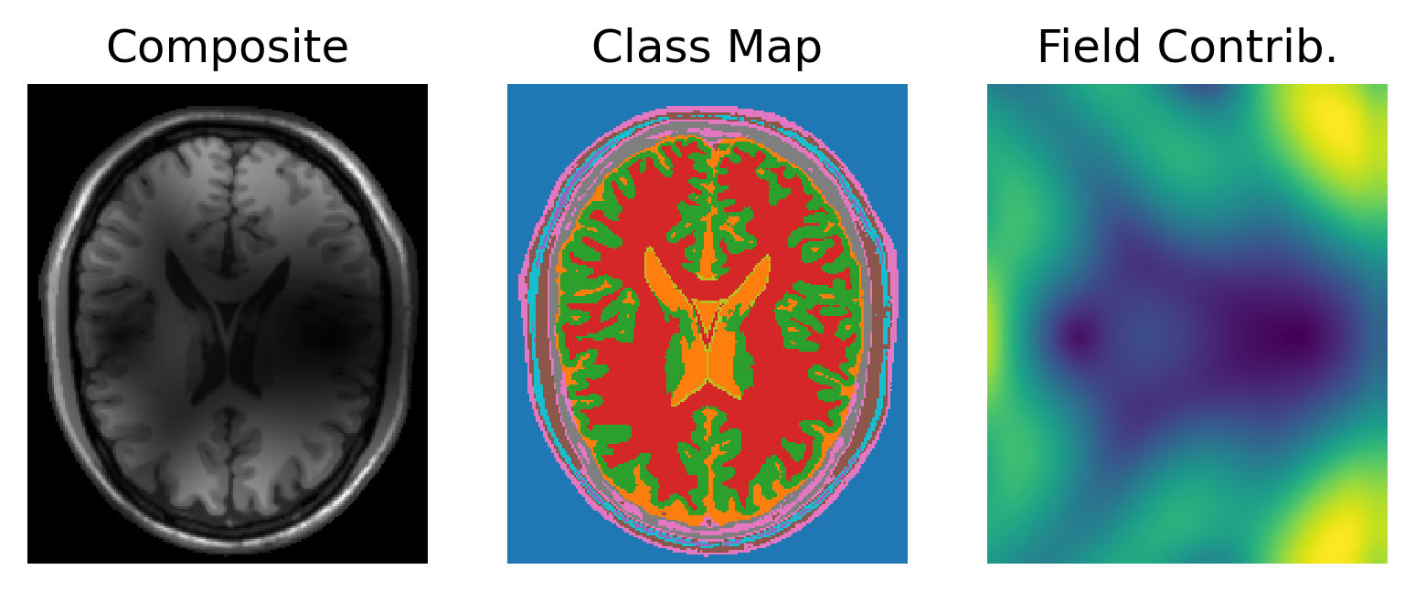
Figure 1: Example of a prominent bias field modifying the BrainWeb Cocosco et al. [1997] phantom.

The MRI bias field problem admits the following multiplicative formulation [Vovk et al., 2007],

$$y(x)=f^{*}(x)\cdot\mu^{*}(x),\quad\text{for}\;x\in\mathcal{X}$$ (5)

where $f^{*}$ is a positive smooth field on $\mathcal{X}$, and $\mu^{*}(x)$ are, by convention, positive tissue values at locations $x\in\mathcal{X}$. Given a fixed number of tissues classes $M$, process (5) can be reformulated as (2) under a $\log$-transformation.

In supervised learning tasks, the visual inconsistencies caused by MRI bias fields present significant challenges, as they prevent the acquisition of accurate ground truth signal information from patient scans. This issue parallels the earlier discussed problem of non-linear ICA, where, again, learning is hampered due to partial information and concerns regarding injectivity.

1.2 Prior Work

To the authors’ best knowledge, the closest work on the theory of continuous and step decompositions is Kim and Tagare [2014], where they provide a characterization of the set of viable functions given an observed composite signal $h^{*}$. The composite $h^{*}=f^{*}\cdot g^{*}$ is assumed to be the product of a positive continuous function $f^{*}$ and a positive step-wise function $g^{*}$. Assuming knowledge of the tissue ratios $\{\mu_{k}/\mu_{k+1}\}_{k=1}^{M-1}$, Kim and Tagare [2014] have shown that one there are scalars $\{a_{k}\}_{k=1}^{M}$ such that the set

$$\widetilde{\mathcal{F}}=\bigl{\{}f:\mathcal{X}\to\mathbb{R}:\forall x\in\mathcal{X},\,f(x)\in\{a_{k}h^{*}(x)\}_{k=1}^{M}\bigr{\}}$$

contains a unique scalar multiple of $f^{*}$. This result is then followed by a practical algorithm which optimizes over a soft-label surrogate of $\widetilde{\mathcal{F}}$.

The theoretical result of Kim and Tagare [2014] is interesting since it dramatically reduces the search space for a viable $f$, esp. when $\mathcal{X}$ is finite. What this result does not tell us is how to identify $f^{*}$ in the set $\widetilde{\mathcal{F}}$, and whether $f^{*}$ is identifiable at all. This issue becomes readily apparent in finite sample scenarios, where there may be multiple ways to construct observations $h^{*}$ from different smooth-and-step pairs $(\tilde{f},\tilde{g})$. In short, the work of Kim and Tagare [2014] does not address the question of identifiability which is a focus of our work. Moreover, when no level information is available, $\widetilde{\mathcal{F}}$ itself is unknown. In this regime, attempts to approximate the set $\widetilde{\mathcal{F}}$ would ultimately be sensitive to initialization choice for scale parameters $\{a_{k}\}_{k}$.

2 Identifiability Theory

Let $\mathcal{F}_{\omega}(\mathcal{X})$ be a vector space of real-valued, uniformly continuous functions with modulus of continuity $\omega:[0,\infty)\to[0,\infty)$ over the metric space $(\mathcal{X},d)$. That is to say,

$$\mathcal{F}_{\omega}(\mathcal{X})=\bigl{\{}f:\mathcal{X}\to\mathcal{Y}:\;\|f(x)-f(x^{\prime})\|\leq\omega(d(x,x^{\prime})),\;\forall x,x^{\prime}\in\mathcal{X}\bigr{\}}.$$ (6)

The results of this section will be presented for outputs in $(\mathbb{R},\,|\cdot|)$, but readers interested in a more general formulation may refer to Appendix A.

We consider the problem of identifying components $(f^{*},\bm{\mu}^{*},\bm{z}^{*})$ from observations

$$y_{i}=f^{*}(x_{i})+\mu^{*}_{z_{i}^{*}},\quad\text{for}\;i=1,\ldots,n,$$ (7)

assuming that $f^{*}$ is an element of the function space $\mathcal{F}_{\omega}(\mathcal{X})$. Given the commutative nature of addition, correctly identifying $(\bm{\mu}^{*},\bm{z}^{*})$ will automatically identify an element of $[f^{*}]_{n}$. In order to recover the true triplet $(f^{*},\bm{\mu}^{*},\bm{z}^{*})$ we consider solving the optimization

$$(\widehat{f},\bm{\widehat{\mu}},\bm{\widehat{z}})=\operatorname*{argmin}_{\begin{subarray}{c}f\in\mathcal{F}_{\omega}(\mathcal{X}),\\ \bm{\mu}\in\mathbb{R}^{M},\;\bm{z}\in[M]^{n}\end{subarray}}\;\frac{1}{n}\sum_{i=1}^{n}(y_{i}-\mu_{z_{i}}-f(x_{i}))^{2},$$ (8)

and its zero-mean version where a constraint is added ensuring that $f$ is empirically zero-mean, i.e., $\sum_{i=1}^{n}f(x_{i})=0$. This zero-mean constraint addresses issues analogous to the scalar multiple problem described by Kim and Tagare [2014]. By providing conditions under which (8) unambiguously recovers the sampled clusters $\{\mu_{z_{i}^{*}}^{*}\}_{i}$, we will have shown identifiability for the step and smooth decomposition (7).

We start by recalling the definition of a $\rho$-neighbor graph associated with a point cloud $X=\{x_{i}\}_{i=1}^{n}$ lying in a metric space $(\mathcal{X},d)$:

Definition 1 (Neighbor Graph).

The $\rho$-neighbor graph $G_{\rho}(X)$ of point cloud $X=\{x_{i}\}$ is the graph with vertex set $[n]$ and edge set

$$\bigl{\{}(i,j)\in[n]^{2}:\,i\neq j\;{\rm and}\;d(x_{i},x_{j})\leq\rho\bigr{\}}.$$

The $\rho$-neighbor graph captures some aspect of the topology of the point cloud. Paired with the modulus of continuity $\omega$, this graph allows us to quantify long-range variation of a particular $f^{*}\in\mathcal{F}_{\omega}(\mathcal{X})$ via its local variations along the edges. Control over $\mathcal{F}_{\omega}(\mathcal{X})$, and by extension $f^{*}$, will rely on the connectedness of $G_{\rho}(X)$ and the size of the neighborhood distance $\rho$. Therefore, to every point cloud $X$, we associate a connectivity parameter:

Definition 2 (Connectivity).

For a point cloud $X$, the connectivity is defined as

$$\rho_{\min}(X):=\inf\bigl{\{}\rho>0:\;\text{$G_{\rho}(X)$ is connected}\bigr{\}}.$$

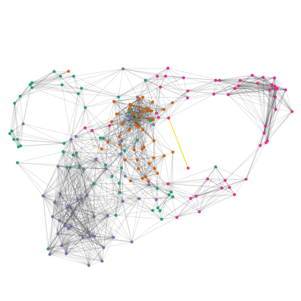
(a) $\rho$-neighbor connectivity graph

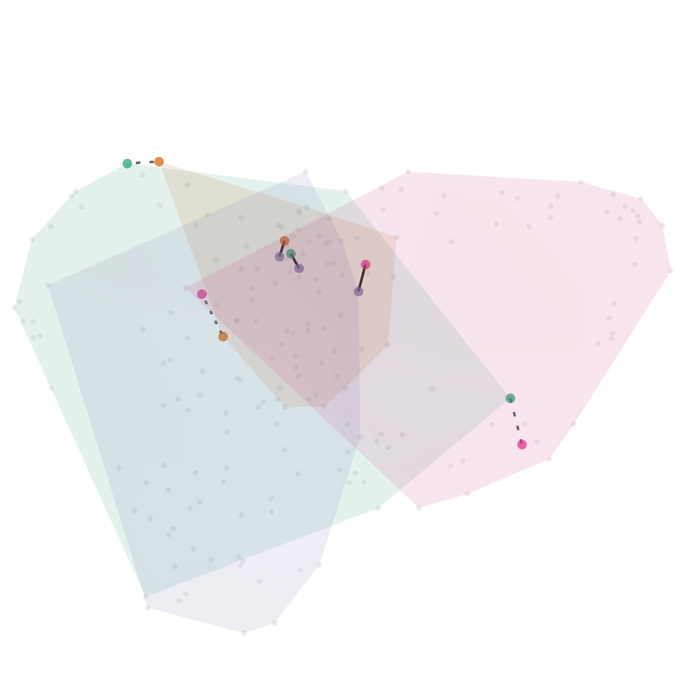
(b) Cluster connectivity graph

Figure 2: A $\rho$-neighbor and cluster connectivity graph on UMAP-reduced features for four topics from the “20 Newsgroups” classification dataset. Highlighted in gold in the left subfigure is an edge with length equal to connectivity $\rho_{{\rm min}}$. Drawn in black in the right subfigure are the corresponding cluster distance edges $d(\mathcal{C}_{k},\mathcal{C}_{\ell})$. Cluster graph edges which are larger than $\delta_{\rm lbd}$ are drawn in dashed. The final cluster graph $G_{\delta_{\rm lbl}}(\mathcal{C})$ is a tree with a connecting hub at the blue colored cluster.

Similar to how $\rho_{\min}(X)$-neighbor graph associates deviations in the smooth component $f^{*}$ with traversals between neighboring nodes in the point cloud, we associate deviations in the step component with traversals along the edges of a graph. This graph’s nodes represent clusters induced by $\bm{z}^{*}$, namely, $\mathcal{C}=\{\mathcal{C}_{k}\}_{k\in[M]}$ where $\mathcal{C}_{k}=\{i\in[n]:z^{*}_{i}=k\}$ is the cluster corresponding to label $k$. Traversal between clusters will be measured with respect to the following cluster distance:

$$d(\mathcal{C}_{k},\mathcal{C}_{\ell})\coloneqq\min_{i\in\mathcal{C}_{k},\,j\in\mathcal{C}_{\ell}}d(x_{i},x_{j}).$$ (9)

The pairwise distances of $\mathcal{C}$, although not corresponding to a metric space, can be used with a tolerance $\delta>0$ to construct a neighbor graph $G_{\delta}(\mathcal{C})$, with the edge set

$$\bigl{\{}(\mathcal{C}_{k},\mathcal{C}_{\ell}):\;k\neq\ell\;\text{and}\;\;d(\mathcal{C}_{k},\mathcal{C}_{\ell})\leq\delta\bigr{\}}.$$

Definition 3 (Label distance).

The label distance for paired data $(X,\bm{z}^{*})$ is

$$\delta_{\rm lbl}(X,\bm{z}^{*})\coloneqq\inf\bigl{\{}\delta>0:\;\text{$G_{\delta}(\mathcal{C})$ is connected}\bigr{\}}.$$ (10)

When clear from context, dependence on sample $(X,\bm{z}^{*})$ will be omitted from all defined terms. Figure 3 shows an example of a $\rho$-neighbor graph and the associated quantities.

Our main result is the following cluster recovery guarantee:

Theorem 1 (Cluster recovery).

Let $X=\{x_{i}\}_{i=1}^{n}$ be a point cloud in a metric space $(\mathcal{X},d)$ and let $\{y_{i}\}_{i=1}^{n}$ follow model (7)with $f^{*}\in\mathcal{F}_{\omega}(\mathcal{X})$ and $\bm{z}^{*}\in[M]^{n}$. If the connectivity $\rho_{\min}$ of $X$ satisfies

$$\omega(\rho_{\min})<\frac{1}{2M}\min_{k\neq\ell}|\mu_{k}^{*}-\mu_{\ell}^{*}|,$$ (11)

then, the labels $\bm{\widehat{z}}$ produced by (8) have zero misclassification error relative to $\bm{z}^{*}$.

Our next result is an error bound on the recovered levels $\bm{\widehat{\mu}}$:

Proposition 1 (Level recovery).

Under the assumptions of Theorem 1, let $(\widehat{f},\bm{\widehat{\mu}},\bm{\widehat{z}})$ be the solution of the zero-mean version of problem (8). Then, we have

$$\max_{k\in[M]}|\mu_{k}^{*}-\widehat{\mu}_{k}|\leq 2(M-1)\,\omega(\delta_{\rm lbl})+\Bigl{|}\frac{1}{n}\sum_{i=1}^{n}f^{*}(x_{i})\Bigr{|}.$$ (12)

In essence, both Theorem 1 and Proposition 1 provide deviation bounds under specific connectivity constraints. The quantities $\rho_{\min}$ and $\delta_{\rm lbl}$ gauge the minimum jump distances at which the induced graphs of $\{x_{i}\}_{i=1}^{n}$ and $\{\mathcal{C}_{k}\}_{k=1}^{M}$ remain connected. The modulus $\omega(\cdot)$ then translates these jumps in distances into equivalent jumps in levels, observed indirectly through $\{y_{i}\}$.

Theorem 1 says that perfect cluster recovery $\bm{\widehat{z}}\equiv\bm{z}^{*}$ is attainable if this translated jump is roughly below the minimum resolution of the true levels $\{\mu^{*}_{k}\}$. Proposition 1 has a similar theme, but in the context of level recovery, where the possible values of $\mu_{k}^{*}\in\mathbb{R}$ are not discretized. This leads to a gradual reduction in error as outlined in Proposition 1, contrasting with the sharp recovery of discrete labels $z_{i}^{*}\in[M]$ in Theorem 1.

The remainder term $|\frac{1}{n}\sum_{i}f^{*}(x_{i})|$ in (12) highlights the scalar-shift ambiguity inherent in the components of model (7), where for any scalar $c\in\mathbb{R}$ we can rewrite (7) as

$$y_{i}=(f^{*}(x_{i})-c)+(\mu^{*}_{z_{i}^{*}}+c).$$

In other words, the two components are only identifiable up to a scalar shift. More generally, problem (8) can be extended to include a constraint $\frac{1}{n}\sum_{i=1}^{n}f(x_{i})=\macc@depth\char 1\relax\frozen@everymath{\macc@group}\macc@set@skewchar\macc@nested@a 111{f}$, for some prescpecified average value $\macc@depth\char 1\relax\frozen@everymath{\macc@group}\macc@set@skewchar\macc@nested@a 111{f}$, in which case Proposition 1 holds with the remainder term $|\frac{1}{n}\sum_{i}f^{*}(x_{i})-\macc@depth\char 1\relax\frozen@everymath{\macc@group}\macc@set@skewchar\macc@nested@a 111{f}|$.

As an immediate corollary to Proposition 1, one can show that, under mild regularity on the sampling of $(X,\bm{z}^{*})$, the zero-mean recovery problem (8) achieves asymptotic identifiability of $(\bm{\mu}^{*},\bm{z}^{*})$. As this corollary references multiple sets of samples, the notation $(\cdot)^{(n)}$ will be used to differentiate parameters belonging to different sets of observations $\{y_{i}\}_{i}$. We also allow the number of observed levels $M_{n}$ to grow with $n$. We say that a condition is eventually satisfied if it holds for all $n\geq N$ for some $N\in\mathbb{N}$.

Corollary 1.

Consider a sequence of point clouds $\{X^{(n)}\}$, with corresponding true labels $\{\bm{z}^{*(n)}\}$ and class levels $\bm{\mu}^{*(n)}\in\mathbb{R}^{M_{n}}$. Let $\delta_{\rm lbl}^{(n)}$ be the label distance for $(X^{(n)},\bm{z}^{*(n)})$. Assume that the connectivity condition (11) is eventually satisfied, and as $n\to\infty$,

$$\omega(\delta_{\rm lbl}^{(n)})=o(M_{n}^{-1}),\quad\frac{1}{n}\sum_{x\,\in\,X^{(n)}}f^{*}(x)=o(1).$$

Then for any solution $(\widehat{f}^{(n)},\bm{\widehat{\mu}}^{(n)},\bm{\widehat{z}}^{(n)})$ of the zero-mean version of problem (8),

$$\lim_{n\rightarrow\infty}\max_{k\in M_{n}}\bigl{|}\mu_{k}^{*(n)}-\widehat{\mu}_{k}^{(n)}\bigr{|}=0.$$

According to Corollary 1, when $\{M_{n}\}$ is bounded, a set of sufficient conditions for recovery of both clusters and levels is:

$$\rho_{\min}^{(n)}=o(1),\quad\delta_{\rm lbl}^{(n)}=o(1),\quad\text{and}\quad\Delta_{n}:=\min_{k\neq\ell}|\mu_{k}^{*(n)}-\mu_{\ell}^{*(n)}|=\Omega(1),$$

i.e., minimum level gap is bounded below. When $\{M_{n}\}$ is unbounded, both the connectivity $\rho_{\min}$ and the label distance $\delta_{\rm lbl}$ must decrease more rapidly. For example, when the smooth component is Lipschitz (i.e., $\omega(t)=Lt$), a set of sufficient conditions are

$$\rho_{\min}^{(n)}=o(\Delta_{n}/M_{n}),\quad\delta_{\rm lbl}^{(n)}=o(1/M_{n}).$$

Note that Corollary (11) is a deterministic result, but it can be translated to a high probability version given appropriate assumptions on the sampling distribution of $(X,\bm{z})$.

The identifiability results of this section are intuitive and described in terms of easily understood topological quantities. However, it is noteworthy that how to obtain a perfect classification result similar to Theorem 1 is not immediately clear. That is, irrespective of the placements of labels $\bm{z}^{*}$ on the point cloud $X$, and regardless of the dimension of the space carrying $X$, we have shown that one can globally control $\bm{\widehat{z}}$ using only a scalar parameter of the point cloud, namely, the radius of connectivity of its associated neighbor graphs $G_{\rho}(X)$.

3 Methods and Optimization

For practical estimation, we consider estimating functions $f^{*}\in\mathbb{H}$ lying in the Hilbert-norm $R$-ball of an RKHS. The following example shows that this case can be treated as a special case of (6) with a linear modulus $\omega(t)=O(t)$.

Example 1.

Consider the case where $f^{*}$ lies in RKHS $\mathbb{H}$. The natural metric to consider on $\mathcal{X}$ is the so-called kernel metric

$$d_{\mathcal{K}}(x,x^{\prime}) :=\|\mathcal{K}(x,\cdot)-\mathcal{K}(x^{\prime},\cdot)\|_{\mathbb{H}}=\sqrt{\mathcal{K}(x,x)-2\mathcal{K}(x,x^{\prime})+\mathcal{K}(x^{\prime},x^{\prime})}.$$ (13)

Using the Cauchy–Schwarz inequality, it is straightforward to show the following Lipschitz property: For any $f\in\mathbb{H}$, we have

$$|f(x)-f(x^{\prime})|\leq\|f\|_{\mathbb{H}}\,d_{\mathcal{K}}(x,x^{\prime})$$

for all $x,x^{\prime}\in\mathcal{X}$. Letting $\omega_{f}$ denote a modulus of continuity of function $f$, the above shows that one can take $\omega_{f}(t)=\|f\|_{\mathbb{H}}\cdot t$ for all $f\in\mathbb{H}$. If we further assume $\|f^{*}\|_{\mathbb{H}}\leq R$ for some constant $R$, then $\omega(t)=O(t)$.

AltMin Algorithm

For our estimation procedure, we propose a blockwise coordinate descent with alternating updates on $(\bm{\mu},\bm{z})$ and $f$. More specfically, in each iteration, the current estimates $(\widehat{f},\bm{\widehat{\mu}},\bm{\widehat{z}})$ are updated to the new ones $(\widehat{f}^{+},\bm{\widehat{\mu}}^{+},\bm{\widehat{z}}^{+})$ by

$$\widehat{f}^{+}=\operatorname*{argmin}_{f\in\mathbb{H}}\frac{1}{n}\sum_{i=1}^{n}(y_{i}-\widehat{\mu}_{\widehat{z}_{i}}-f(x_{i}))^{2}+\tau\|f\|_{\mathbb{H}}^{2},$$ (14)

$$(\bm{\widehat{\mu}}^{+},\bm{\widehat{z}}^{+})=\operatorname*{argmin}_{\bm{\mu}\in\mathbb{R}^{M},\,\bm{z}\in[M]^{n}}\frac{1}{n}\sum_{i=1}^{n}(y_{i}-\mu_{z_{i}}-\widehat{f}^{+}(x_{i}))^{2},$$ (15)

with $\tau$ and $M$ being values to be determined through a cross-validation procedure.

For fixed $\widehat{f}$, optimization (15) can be solved through a $k$-means procedure. For RKHS $\mathbb{H}$ equipped with kernel $\mathcal{K}:\mathcal{X}\times\mathcal{X}\rightarrow\mathbb{R}$, optimization (14) has the following representer solution

$$\widehat{f}^{+}=\frac{1}{\sqrt{n}}\sum_{i=1}^{n}\widehat{\alpha}^{+}_{i}\mathcal{K}(x_{i},\cdot),\;\;\bm{\widehat{\alpha}^{+}}:=(K+\tau I_{n})^{-1}(\bm{y}-\widehat{Z}\bm{\widehat{\mu}})/\sqrt{n}$$ (16)

where $K$ is the $n\times n$ kernel matrix with entries $K_{ij}=\mathcal{K}(x_{i},x_{j})/n$ and $\widehat{Z}\in\{0,1\}^{n\times L}$ is the one-hot encoding label matrix for previous label estimate $\bm{\widehat{z}}$.

3.1 One-step Analysis

In general, the interaction between updates (14) and (15) may be quite complicated. In this section we show a positive result: In the large sample limit, classification with AltMin simplifies to classification with regular $k$-means on the uncontaminated (step) signal.

We consider observations $\{y_{i}\}_{i}$ drawn from (1) with i.i.d. zero-mean noise $\varepsilon_{i}$ of variance $\sigma^{2}$. As before, $g^{*}$ will be assumed to be a step signal with $g^{*}(x_{i})=\mu_{z_{i}^{*}}^{*}$, although the results of this section hold for any $g^{*}$ that is sufficiently outside the RKHS, as will be made precise in Corollary 2. For our analysis, we consider a half-step of the AltMin algorithm, evaluating performance after update (16). Our goal is to show the pointwise consistency of the KRR estimator $\bm{\widehat{f}}\coloneqq(\widehat{f}(x_{i}))$, that is

$$\lim_{n\to\infty}\mathbb{E}_{\bm{\varepsilon}}\,{\rm MSE}(\bm{f}^{*},\bm{\widehat{f}})=0,$$ (17)

where ${\rm MSE}(\bm{a},\bm{b})=\|\bm{a}-\bm{b}\|_{2}^{2}/n.$

Let $K=V\Lambda V^{\mathsf{T}}$ be the eigenvalue decomposition of the kernel matrix where $\Lambda=\operatorname{diag}(\lambda_{i},i\in[n]$), and define

$$h(\lambda;\tau):=\frac{\lambda^{2}}{(\lambda+\tau)^{2}},\quad\Gamma_{\tau}:=\sqrt{h(\Lambda;\tau)}=\Lambda(\Lambda+\tau I)^{-1}$$

extending a scalar function to diagonal matrices in the natural way (i.e., by applying to each diagonal entry.) We assume the eigenvalues are ordered as follows: $\lambda_{1}\geq\lambda_{2}\geq\cdots\geq\lambda_{n}$. Consider the Fourier expansion of $f^{*}$ and $g^{*}$ in the (empirical) eigen-basis of the kernel, that is, $\bm{\breve{f}}\coloneqq(\breve{f}_{i})\coloneqq V^{\mathsf{T}}\bm{f}^{*}$ and $\bm{\breve{g}}\coloneqq(\breve{g}_{i})\coloneqq V^{\mathsf{T}}\bm{g}^{*}$. Then

$$\frac{1}{n}\mathbb{E}_{\bm{\varepsilon}}\|\bm{f}^{*}-\bm{\widehat{f}}\|_{2}^{2} =\frac{1}{n}\mathbb{E}_{\bm{\varepsilon}}\|(I_{n}-\Gamma_{\tau})V^{\mathsf{T}}\bm{f}^{*}-\Gamma_{\tau}V^{\mathsf{T}}\bm{g}^{*}-V^{\mathsf{T}}\bm{\varepsilon}\|_{2}^{2}$$

$$\leq\frac{2}{n}\|(I_{n}-\Gamma_{\tau})\bm{\breve{f}}\|_{2}^{2}+\frac{2}{n}\|\,\Gamma_{\tau}\bm{\breve{g}}\,\|_{2}^{2}+\frac{\sigma^{2}}{n}{\rm tr}(\Gamma_{\tau}^{2})$$

$$=\frac{2}{n}\sum_{i=1}^{n}\frac{\tau^{2}\breve{f}_{i}^{2}}{(\lambda_{i}+\tau)^{2}}+\frac{2}{n}\sum_{i=1}^{n}h(\lambda_{i};\tau)\,\breve{g}_{i}^{2}+\frac{\sigma^{2}}{n}\sum_{i=1}^{n}\frac{\lambda_{i}^{2}}{(\lambda_{i}+\tau)^{2}}$$ (18)

The first and the third terms are the bias and variance, respectively, for recovering $\bm{f}^{*}$ in classical kernel ridge regression (KRR). Both can be made to go to zero as $n\to\infty$ for a proper choice of $\tau=\tau_{n}=o(1)$. The middle term is new to our decomposition, and is the filtering effect of KRR on the step component $g^{*}(\cdot)$.

Intuitively, since a discontinuous $g^{*}$ is not in the RKHS, one would have

$$\min_{\begin{subarray}{c}\bar{g}\in\mathbb{H}:\\ (\bar{g}(x_{i}))=\bm{g}^{*}\end{subarray}}\|\bar{g}\|_{\mathbb{H}}\to\infty\quad\text{as }n\to\infty.$$

This in turn implies $\frac{1}{n}\sum_{i=1}^{n}\breve{g}_{i}^{2}/\lambda_{i}\to\infty$, forcing the middle term in (18) to become negligible, implying that KKR effectively filters out $g^{*}$. To see this, note that since $\lambda_{i}$ are decaying as a function of $i$, for the expression $\frac{1}{n}\sum_{i=1}^{n}\breve{g}_{i}^{2}/\lambda_{i}$ to grow without bound, most of the energy of $g^{*}$ (where “energy” is defined as $\frac{1}{n}\sum_{i=1}^{n}\breve{g}_{i}^{2}$) must be concentrated on the higher-index components, which correspond to smaller eigenvalues. Multiplication by $h(\lambda_{i},\tau)$ filters out components of $g^{*}$ associated with small eigenvalues; equivalently it acts a a low-pass filter, filtering out higher index (i.e., higher frequency) components.

To make the above intuition more precise, consider the spectral survival function of $g^{*}$:

$$S_{g^{*}}(t):=\sum_{i=1}^{n}\frac{\breve{g}_{i}^{2}}{n}\cdot 1\{\lambda_{i}>t\}.$$ (19)

As $t\to\infty$, $S(t)$ goes to zero, and the faster this decay, the more $g^{*}$ is concentrated on higher-index components. That is, the tail behavior of $S_{g^{*}}(t)$ is what determines how well $g^{*}$ is filtered by KRR. Let $r_{n}=\max\{i\in[n]:\,\breve{g}_{i}^{2}>0\}$ and let $\beta_{n}$ be the largest $\beta\geq 0$ that satisfies

$$S_{g^{*}}(t)\;\leq\;\|\bm{g}^{*}\|_{\infty}^{2}\cdot\Bigl{(}\frac{\lambda_{r_{n}}}{t}\Bigr{)}^{\beta},\quad\text{ for all $t>0$.}$$ (20)

Such a tail bound always exists, since the trivial case $\beta=0$ reduces to $\|\bm{g}^{*}/\sqrt{n}\|_{2}^{2}\leq\|\bm{g}^{*}\|_{\infty}^{2}$. The parameters of the tail bound are influenced by how much the higher-index components of $\bm{\breve{g}}$ contribute to the total norm (or energy). The tail bound works together with the spectral filter $h(\lambda;\tau)$ to give the following control for the middle term of (18):

Proposition 2.

Consider KRR with regularization parameter $\tau_{n}$ and let $\xi_{n}:=\lambda_{r_{n}}/\tau_{n}$. Then,

$$\frac{1}{n}\sum_{i=1}^{n}h(\lambda_{i};\tau_{n})\,\breve{g}_{i}^{2}\;\lesssim\;\max\{\xi_{n}^{2},\,\xi_{n}^{\beta_{n}}\},$$ (21)

where $\lesssim$ denotes inequality up to universal constants.

We note that the best case scenario in Proposition 2 is obtained when $r_{n}=n$ and $\beta_{n}\geq 2$, leading to the quickest possible decay of $O(\xi_{n}^{2})=O((\lambda_{n}/\tau_{n})^{2})$ for the residual norm.

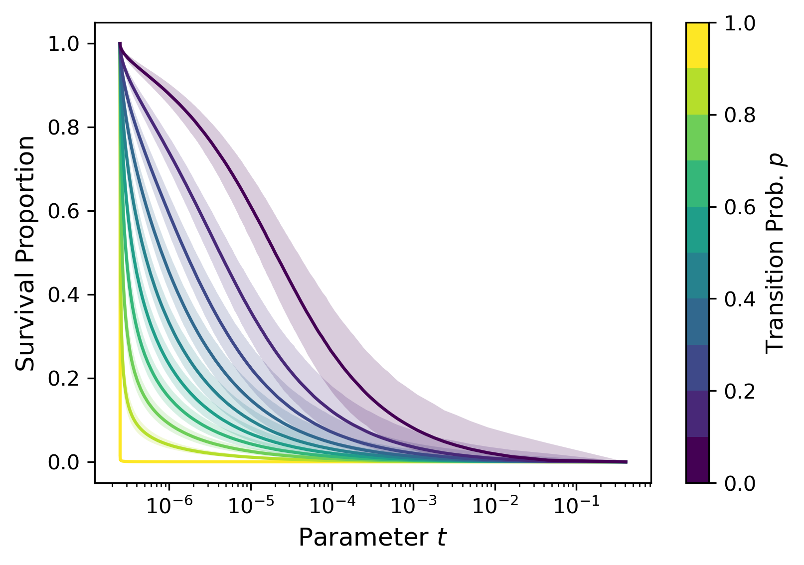
(a) Survival functions of $\bm{\breve{g}}$ for length $n=1000$.

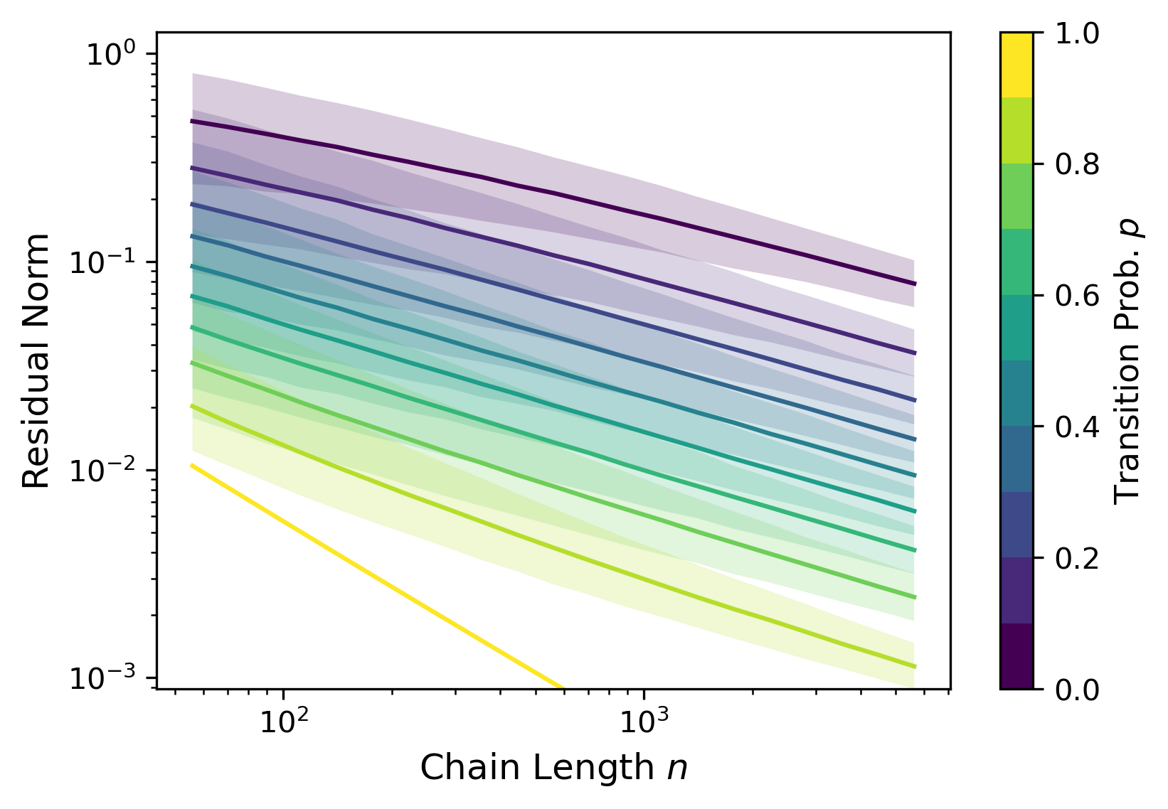
(b) Residual norm $\frac{1}{n}\|\Gamma_{\tau}\bm{\breve{g}}\|_{2}^{2}$ for $\tau_{n}=\sqrt{\lambda_{n}}$.

Figure 3: Experiment results for the 2-state, $p$-probability Markov chain. 10000 chains were simulated for each $p\in\{k/10\}_{k=1}^{10}$. Shown in subfigures are median results with 95% probability intervals shaded in the corresponding colors. In the case of $p=1$, there is no shading.

Next we consider the case where $\mathcal{X}$ is compact and $\mathcal{K}$ is continuous, that is, kernel $\mathcal{K}$ is a Mercer kernel. Then, under the assumption that $\{x_{i}\}$ are i.i.d. draws, the sampling operator associated with $K$ converges compactly, almost surely, to an integral operator $T_{\mathcal{K}}:L^{2}(\mathcal{X})\to L^{2}(\mathcal{X})$ [von Luxburg et al., 2008, Proposition 11-13]. This in turn implies that as long as $r_{n}\to\infty$, we will have $\lambda_{r_{n}}\to 0$. Combined with Proposition 2, this lead to the following consistency result for the one-step procedure:

Corollary 2.

Consider a Mercer kernel and i.i.d. sample $\{x_{i}\}$. Let the regularization parameter $\tau=\tau_{n}$ be chosen such that the first and third term in (18) go to zero and $\xi_{n}=o(1)$. Further suppose that $\liminf r_{n}/n>0$ and $\liminf\beta_{n}>0$. Then,

$$\lim_{n\to\infty}\mathbb{E}_{\bm{\varepsilon}}\,{\rm MSE}(\bm{f}^{*},\bm{\widehat{f}})=0.$$

To provide intuition for these results, we provide an example analyzing the decay of the spectral survival function $S_{g^{*}}(t)$ in a general two-class signal.

Example 2.

Consider step signal $\bm{g}^{*}\in\{-1,1\}^{n}$ generated from an $n$-length, 2-state Markov chain with transition probability $p$. For estimation, we consider the following RKHS:

$$\mathbb{H}^{1}[0,1]=\bigl{\{}f:[0,1]\to\mathbb{R}\mid\;\text{$f$ is abs. cts., }\;\|\partial_{x}f\|_{L^{2}}<\infty,\;f(0)=0\bigr{\}}.$$ (22)

This RKHS has kernel $\mathcal{K}(x,x^{\prime})=\min(x,x^{\prime})$. In this example, we assume the data is sampled at regularly spaced intervals with $x_{i}=i/n$.

The RKHS $\mathbb{H}^{1}[0,1]$ organizes functions by roughness through the Hilbert-norm $\|f\|_{\mathbb{H}^{1}}=\|\partial_{x}f\|_{L^{2}}$. Hence, signals $\bm{g}^{*}$ produced by chains with high transition probabilities are expected to have a larger corresponding Hilbert-norm and, intuitively, a rapidly decaying spectral survival function. This intuition is corroborated in Figure 3, where the survival function $S_{g^{*}}(t)$ and residual norm $\frac{1}{n}\|\Gamma_{\tau}\bm{\breve{g}}\|_{2}^{2}=\frac{1}{n}\sum_{i=1}^{n}h(\lambda_{i};\tau_{n})\,\breve{g}_{i}^{2}$ are plotted for various transition probabilities. One observes that as the transition probability increases, the tail decay of the survival function becomes sharper (Figure 3(a)) and the norm decay steeper (Figure 3(b)).

The kernel matrix $K$ in this case has minimum eigenvalue $\lambda_{n}\approx(4n)^{-1}$. For the regularization choice $\tau_{n}=\sqrt{\lambda_{n}}$ shown in Figure 3(b), the quickest rate of decay guaranteed by Proposition 2—namely, $\mathcal{O}((\lambda_{n}/\tau_{n})^{2})$—will be on the order of $\mathcal{O}(n^{-1})$. This rate is attained in the log-log plot of Figure 3(b) where the curve associated with chain transition probability $p=1$ shows a linear slope of $-1$.

Figure 3 also provides evidence that the conditions of Corollary 2 are met for this general signal class. The survival function plots in Figure 3(a) show natural tail decays for all probabilities $p$ at $n=1000$ and the stable linear decays of Figure 3(b) show that the $\liminf$ conditions on $r_{n}/n$ and $\beta_{n}$ are attainable for a general signal model.

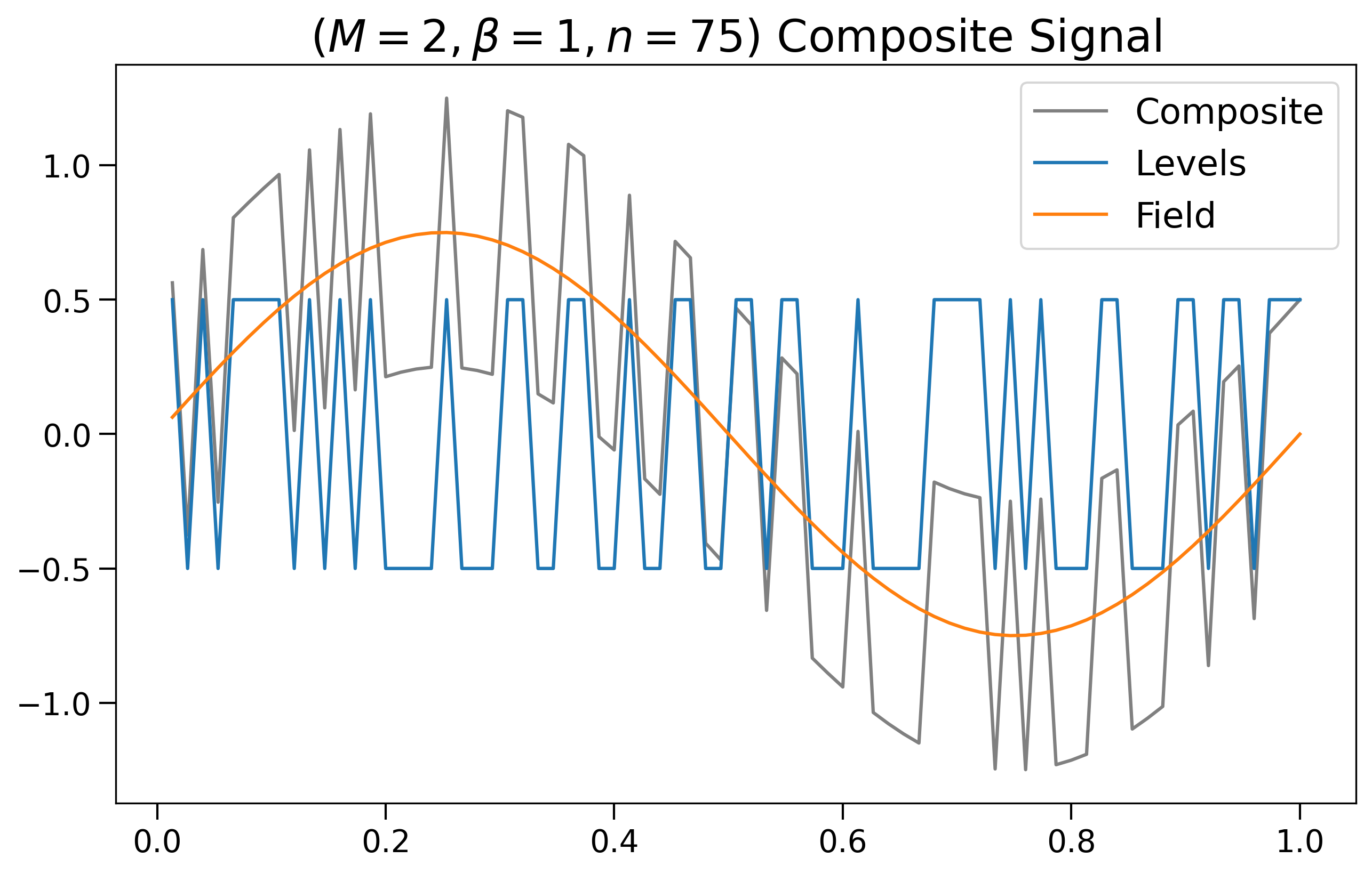
(a) Smoother field

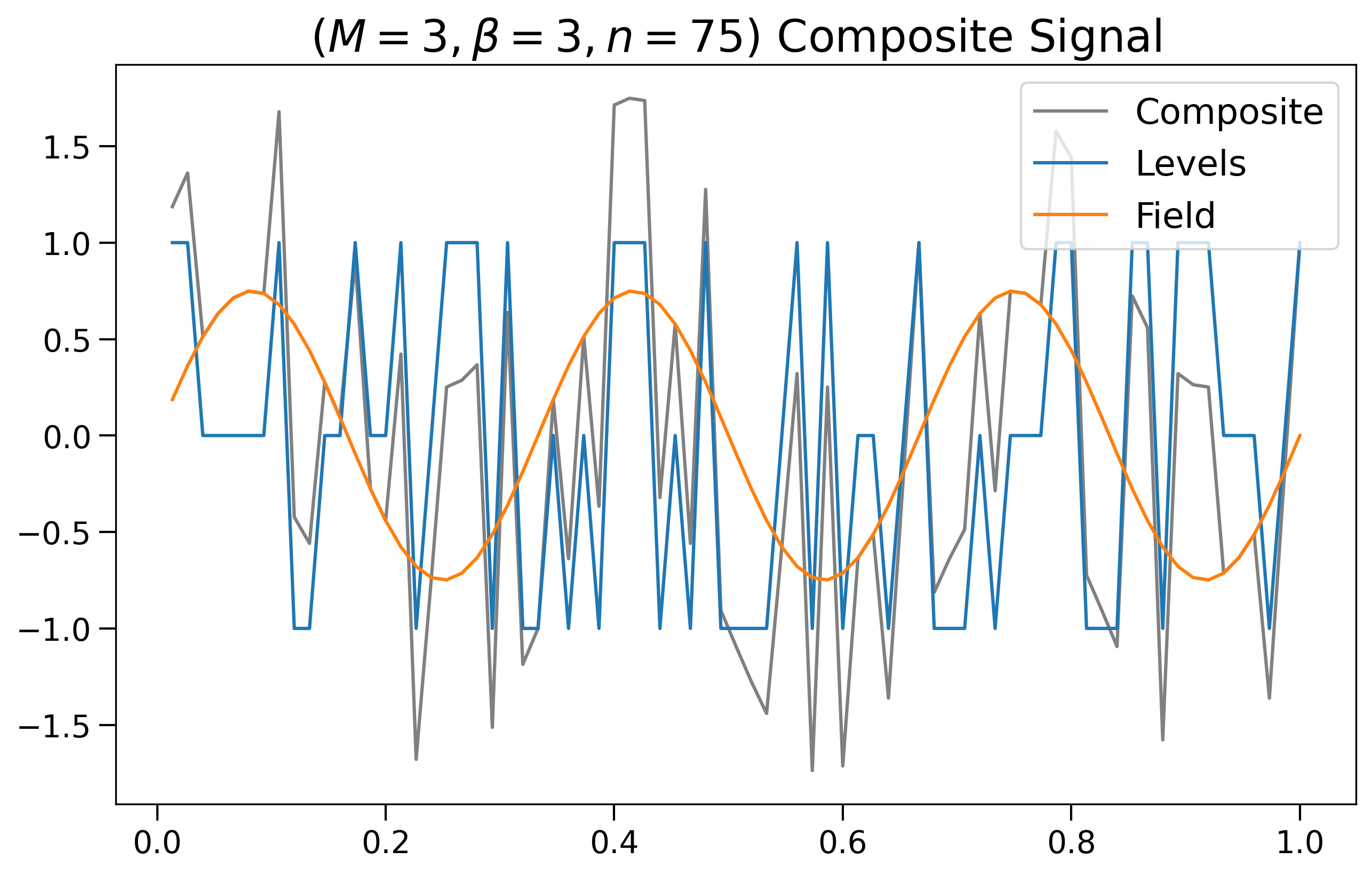
(b) Rougher field

Figure 4: Signal, field and composite observation simulated from (23) for two and three classes.

4 Experiments

We now provide experimental results on the performance of the AltMin algorithm. First, we consider simulated data from an $M$-class data generating process on $\mathcal{X}=[0,1]$ where data $X^{(n)}=\{i/n\}_{i=1}^{n}$ is equispaced, cluster labels $z_{i}^{*}\sim{\rm Unif}([M])$ are uniformly distributed, and the step and smooth components follow

$$\mu_{k}^{*}=k-\frac{M+1}{2},\qquad f_{\beta}^{*}(x)=\frac{3}{4}\,\sin(2\pi\beta x).$$ (23)

The min kernel from Example 2 was chosen for estimation due to its sinusoidal eigenfunctions. Given the equispaced data, the smallest radius $\rho$ that guarantees the connectivity condition of Theorem 1 is

$$\min_{i\neq j}d_{\mathcal{K}}(x_{i},x_{j})=\sqrt{(i+1)/n-2i/n+i/n}=n^{-1/2},$$

where the kernel-metric $d_{\mathcal{K}}(x,x^{\prime})$ was defined in Example 1. The Hilbert-norm of $f^{*}_{\beta}$ can be computed using inner product $\langle f,g\rangle_{\mathbb{H}^{1}}=\int_{0}^{1}\partial_{x}f(x)\,\partial_{x}g(x)\,dx$. Evaluating this norm gives the following worst-case bound on the modulus of continuity of $f^{*}_{\beta}$,

$$\omega(\rho_{\rm min})\leq\|f^{*}_{\beta}\|_{\mathbb{H}^{1}}\cdot\rho_{\rm min}\leq\frac{3\sqrt{2}}{4}\pi\beta\cdot n^{-1/2}.$$ (24)

Finally, a noisy recovery setting will be considered where i.i.d. noise $\varepsilon_{i}\sim\mathcal{N}(0,\sigma^{2})$ is added to mixed observations $f_{\beta}^{*}(x_{i})+\mu_{z_{i}^{*}}^{*}$.

In both recovery settings, sample size is grown in roughly exponential manner starting from $n=25$ to $n=3600$. At each sample size $n$, a total of 100 datasets $(X^{(n)},\bm{y})$ were simulated. Accuracy and deviation results at each $n$ were calculated using the mean score of the 100 datasets.

4.1 Simulation Experiments

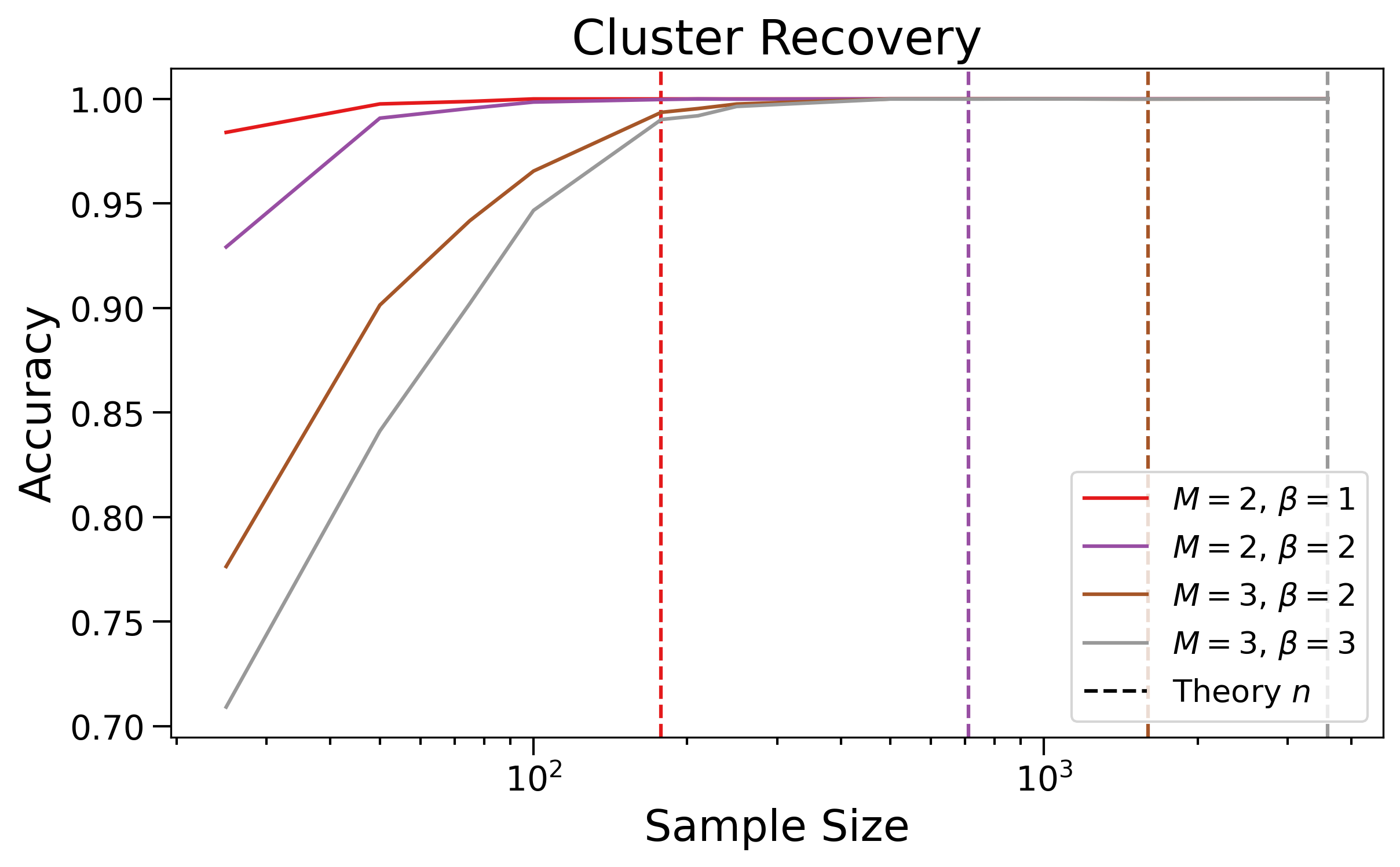
(a) (Noiseless) Classification curves

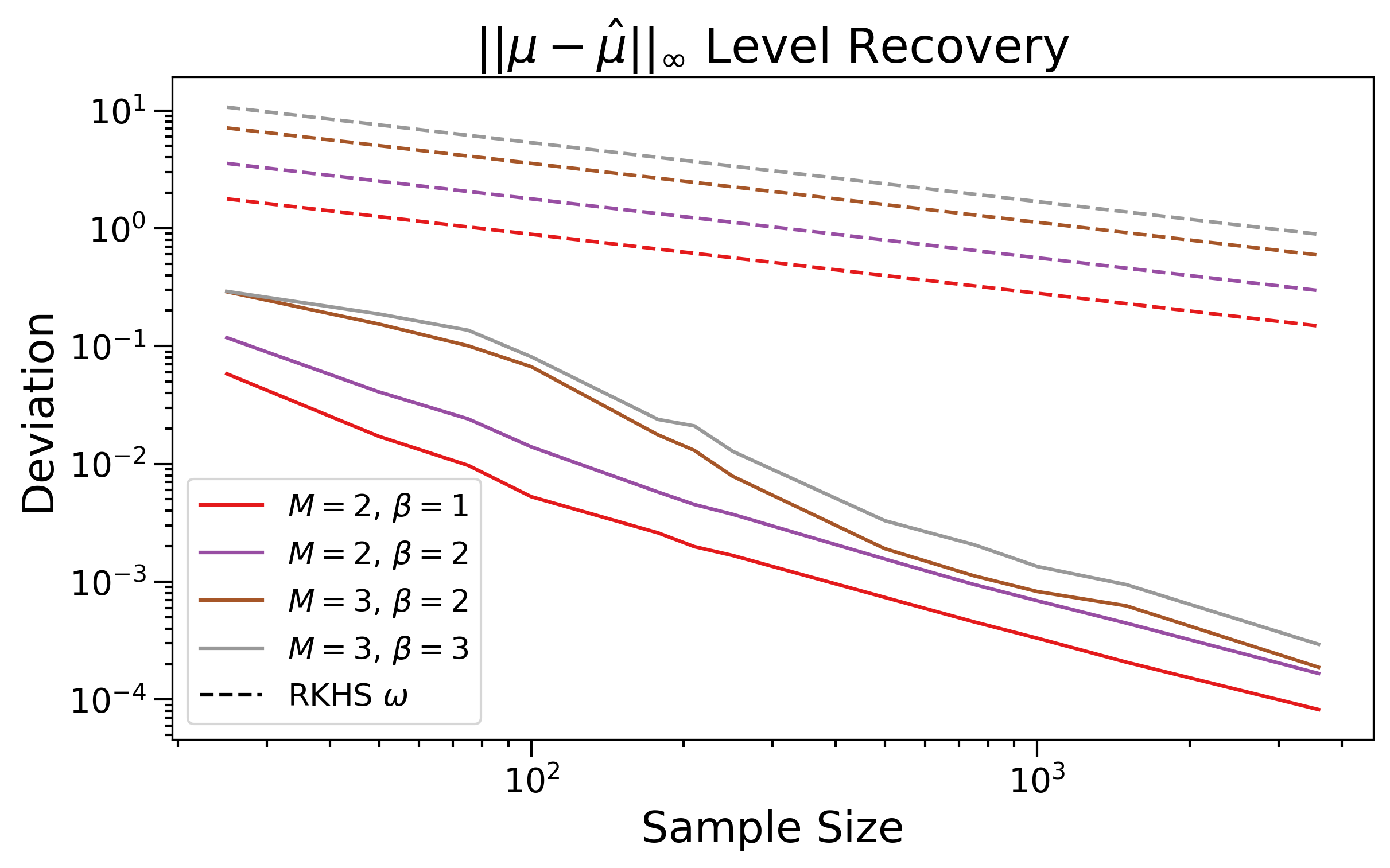
(b) (Noiseless) Deviation curves

Figure 5: AltMin recovery results for a noiseless simulated setting. Worst-case theory bounds are shown as dashed lines for each of the different settings.

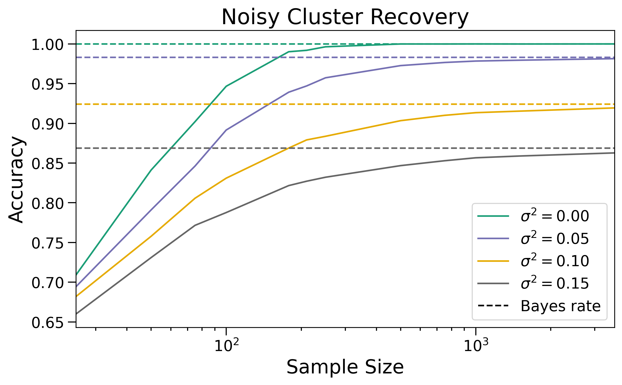
(a) (Noisy) Classification curves

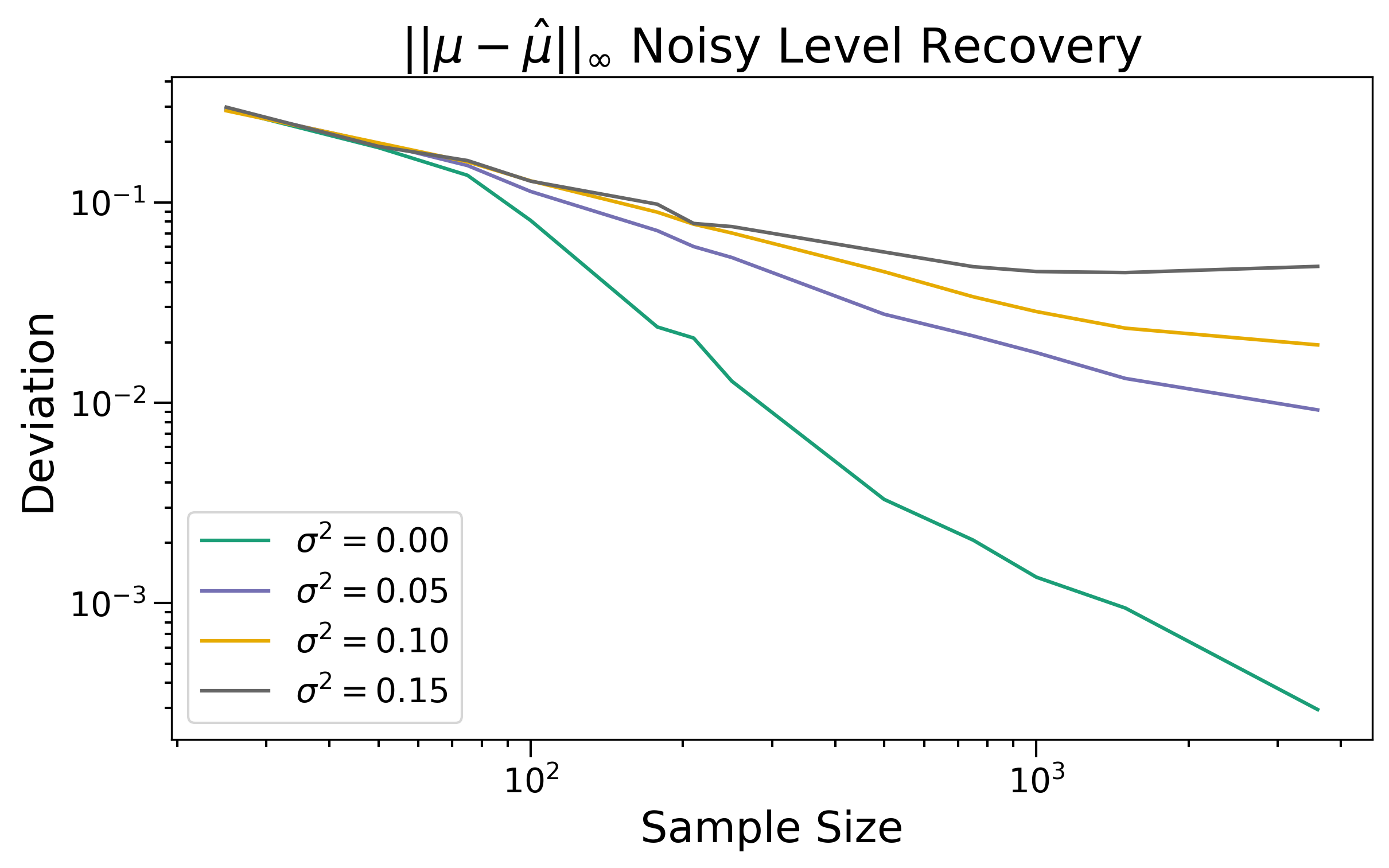
(b) (Noisy) Deviation curves

Figure 6: AltMin recovery results for a noisy simulated setting. Bayes error rates for classification are shown as dashed lines for the various noise levels.

Four settings were considered for noiseless recovery: $(M,\beta)\in\{(2,1),(2,2),(3,2),(3,3)\}$. Cluster recovery and deviation results for the four settings can be found in Figure 5. For each setting of the optimization problem (8), worst-case recovery bounds, shown dashed in Figure 5, were calculated using Theorem 1 and Proposition 1. The AltMin algorithm stays well within these worst-case bounds, demonstrating the effectiveness of the simple blockwise updates for specific problem settings.

For noisy recovery, the setting with $M=\beta=3$ was considered at noise levels $\sigma^{2}\in\{0,\,0.05,\,0.1,\,0.15\}$. Cluster recovery and deviation results for these four settings can be found in Figure 6. In each of the noisy settings, AltMin approaches the Bayes error of what is expected for a perfect classifier.

We note that the rate at which AltMin approaches Bayes error seems faster for the cases where $\sigma^{2}$ is low. This may suggest that the AltMin algorithm is well-suited for smooth field, cluster recovery problems which experience low amounts of background noise.

4.2 MRI Decontamination

For application, we return to the motivating MRI bias field problem. This is a real-world example where the magnitude of the inhomogeneity $f^{*}$ and the tissue intensity $g^{*}$ are much larger than the scale of the background noise $\sigma^{2}$ [Asher et al., 2010]. As we have seen in Section 4.1, this is a type of problem which is a good candidate for the AltMin algorithm.

To make our experiment quantitative, we consider a 4-class, strongly-biased variant of the BrainWeb [Cocosco et al., 1997] phantom. The field estimation step (14) is carried out using a Python spline routine csaps [Prilepin, 2023]. This routine uses an RKHS tensor product of univariate smoothing splines to fit the multidimensional data. Relevant csaps smoothing parameters were selected using a post-fitting process. In practice, smoothing parameters would be selected using a validation set of data which corresponds to a specific coil cluster or MRI scanner.

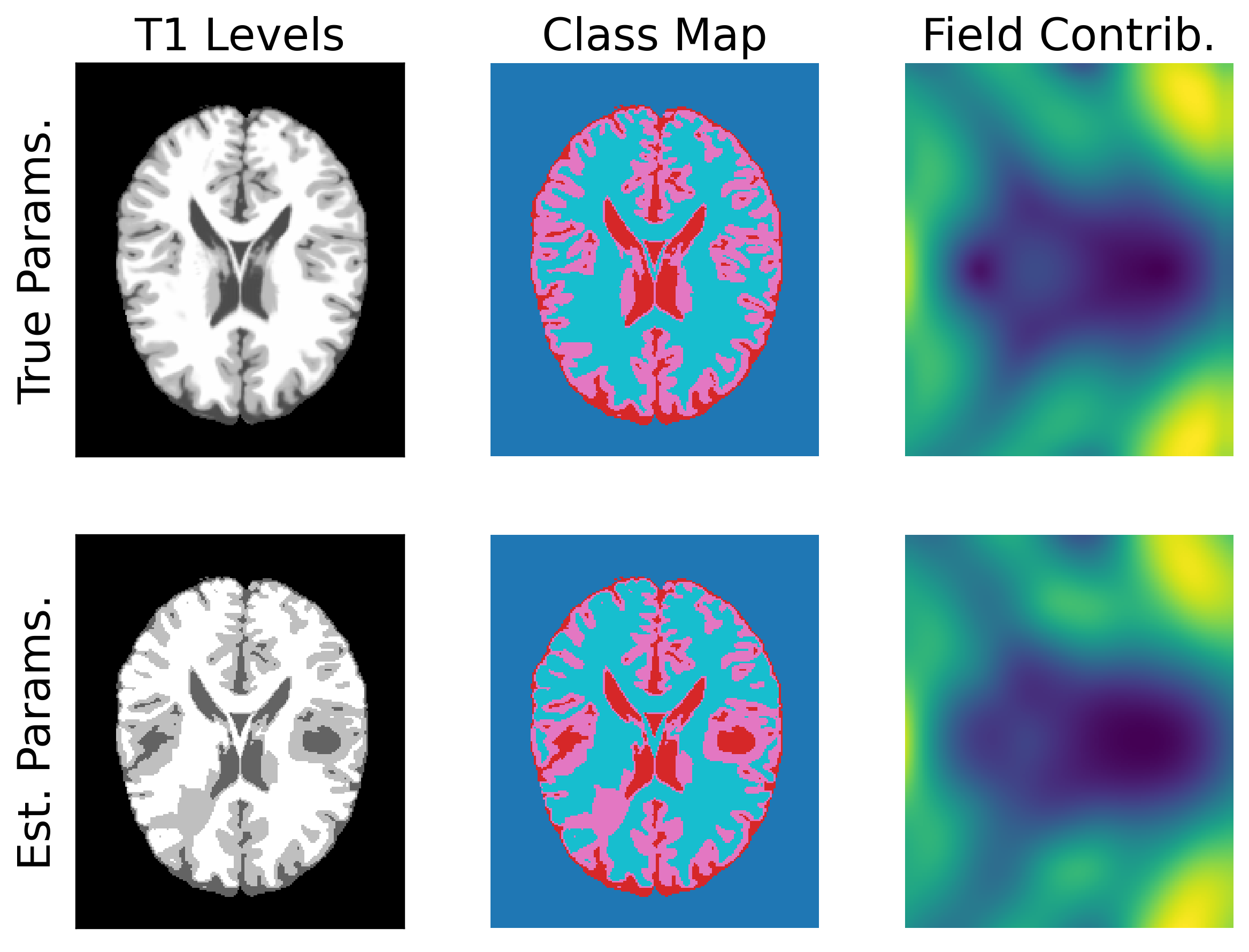
(a) Single sequence recovery

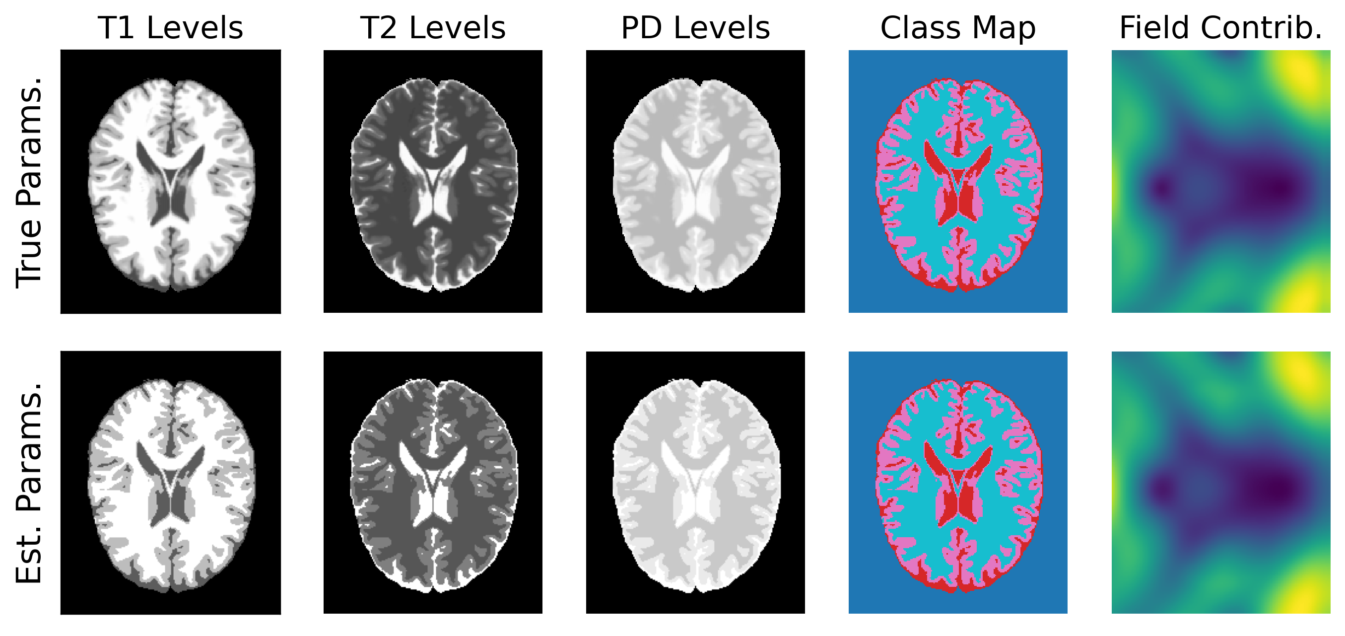
(b) Multi-sequence recovery

Figure 7: AltMin decomposition for the biased BrainWeb dataset. Class maps of the single sequence setting show anomalous tissue patches in areas where the field changes most rapidly.

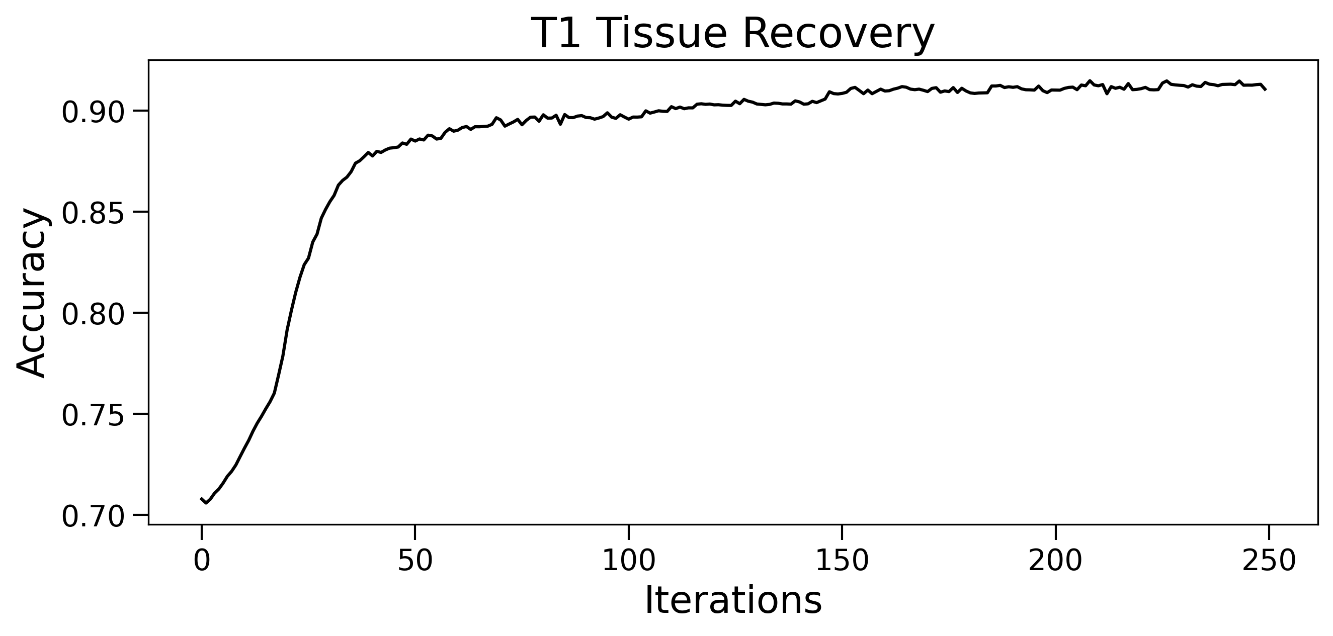
(a) (Single) Accuracy vs. iteration

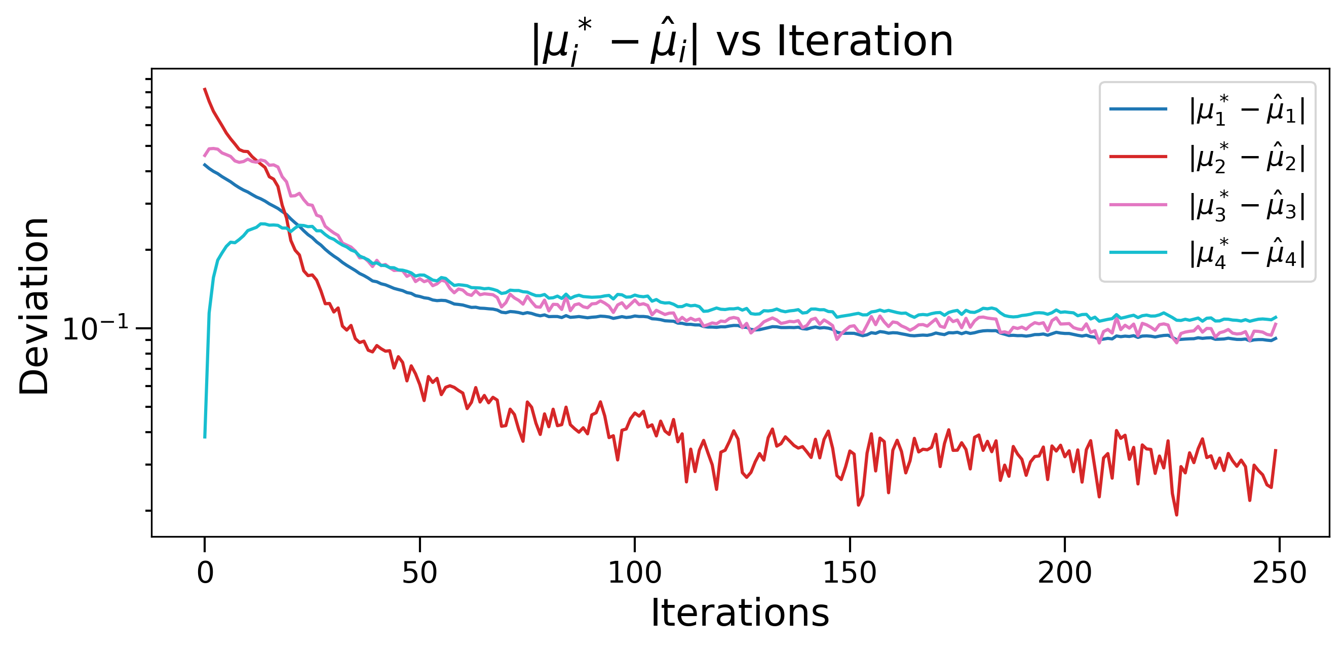
(b) (Single) Deviation vs. iteration

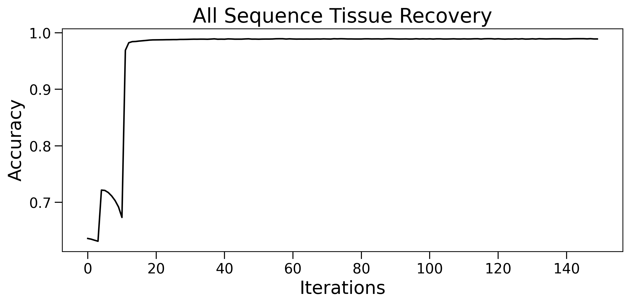
(c) (Multi) Accuracy vs. iteration

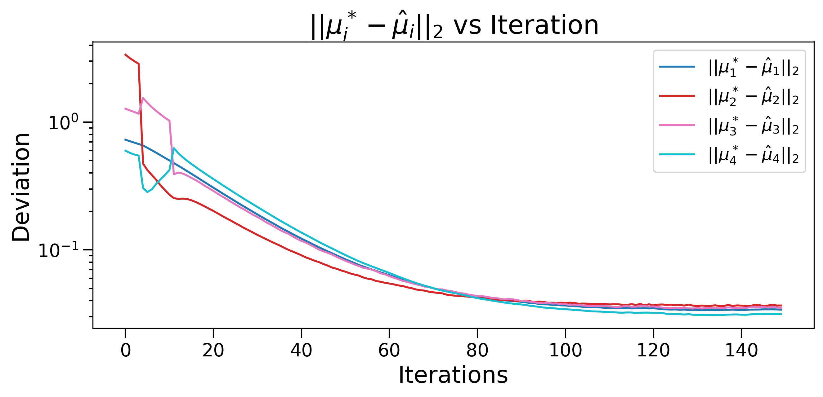
(d) (Multi) Deviation vs. iteration

Figure 8: Cluster and level accuracy of the AltMin algorithm on the biased BrainWeb phantom. Final accuracies for single and multi-sequence settings are 91.07% and 98.91% respectively. Level deviations in the multi-sequence setting are calculated with respect to the vector 2-norm.

For implementation, we consider modeling the bias field for both single sequence and multi-sequence scans. In a multi-sequence scan, it is understood that the bias field does not vary much between sequences [Belaroussi et al., 2006]. For this reason, we consider the following general $p$-sequence data model

$$\bm{y}(x)=f^{*}(x)\cdot\bm{\mu}^{*}(x),\quad\text{for}\;x\in\mathcal{X}$$

where levels $\bm{\mu}^{*}(x)$ take value in $\mathbb{R}^{p}$ and bias $f^{*}(x)$ is still a scalar function.

Bias field and tissue decomposition results for the single and multi-sequence setting can be found in Figure 7 with the respective AltMin optimization results found in Figure 8. The presence of redundant sequencing data, albeit at different intensity scalings, seems to significantly improve AltMin convergence as shown in Figures 8(c)-8(d). This also translate to an improved performance, as many of the anomalous tissue patches seen in Figure 7(a) no longer occur in Figure 7(b). Additional experiments comparing AltMin to other medical debiasing methods can be found in Appendix C.

5 CONCLUSION

In this paper, we defined the problem of composite signal decomposition for continuous contaminants and step-wise signals. We outlined recovery conditions that leverage the local and global topology of the data including: connectivity, minimum true level deviation, and the degree of oscillation of the contaminant. These quantities are natural, and their roles in recovery intuitively clear, allowing for a high-level understanding to be easily derived from our theoretical finding.

Besides identifiability, we developed a practical algorithm AltMin for handling contaminants that reside within an RKHS. This algorithm can be viewed as an extension of both kernel ridge regression (KRR) and $k$-means, with updates to each being performed alternately. MSE bounds for the algorithm were provided in terms of the spectral properties of the data, leading to a “one-step” consistency result in the large sample limit.

We evaluated AltMin empirically on both simulated and real-world data. In the case of simulated data, AltMin operated well within the worst-case theory bounds outlined in Section 2. When the data was further corrupted by noise, AltMin approached the best possible classification rates for the given data generating process. In the real-world study, we conducted an MRI tissue recovery experiment, illustrating how tensor products of smoothing splines can be employed to estimate contaminant MRI bias fields. Given redundant data on the same bias field, AltMin significantly enhanced clustering performance and overall optimization stability.

These empirical studies, alongside the identifiability theory of Section 2, suggest that step-and-smooth decompositions are attainable within worst-case optimality guarantees. Regarding application, the alternating optimization of AltMin appears well-suited for data-dense tasks, especially when data is spatially uniform and low in noise. In this context, decomposition problems akin to MRI multi-sequence recovery could be promising avenues for further applications of the AltMin algorithm.

Appendix A Identifiability Proofs

Any optimal candidate solution $(\widehat{f},\widehat{\mu},\widehat{z})$ to (8) which is fit to data $\{y_{i}\}$ generated from (7) must satisfy

$$f^{*}(x_{i})+\mu^{*}_{z_{i}^{*}}=\widehat{f}(x_{i})+\widehat{\mu}_{\widehat{z}_{i}},\quad\text{for all}\;i\in[n].$$ (25)

Since $\widehat{f}-f^{*}\in\mathcal{F}_{2\omega}(\mathcal{X})$, we may instead analyze the discrepancy

$$g(x_{i})=\mu^{*}_{z_{i}^{*}}-\widehat{\mu}_{\widehat{z}_{i}},\quad\text{for all}\;i=1,\ldots,n,$$

for $g\in\mathcal{F}_{2\omega}(\mathcal{X})$. In addition, we will assume that function $g:\mathcal{X}\rightarrow\mathcal{Y}$ takes values on a normed vector space $(\mathcal{Y},\,\|\cdot\|)$. As a result, the modulus of continuity $\omega$ will be related to the induced norm-metric as $\|g(x)-g(x^{\prime})\|\leq\omega\big{(}d(x,x^{\prime})\big{)}$.

The following result is the main ingredient in the proof of Theorem 1:

Theorem 2.

Suppose for $g\in\mathcal{F}_{2\omega}(\mathcal{X})$ we have $g(x_{i})=\mu^{*}_{z_{i}^{*}}-\widehat{\mu}_{\widehat{z}_{i}}$ for all $i\in[n]$ where $\bm{z}^{*}=(z_{i}^{*})$ and $\bm{\widehat{z}}=(\widehat{z}_{i})$ both belong to $[M]^{n}$. Assume the following holds:

1. $\|\mu^{*}_{k}-\mu^{*}_{\ell}\|\geq\gamma$ for all $k\neq\ell$.

2. $G_{\rho}(X)$ is connected for some $\rho$ with $2\,\omega(\rho)<\gamma/M$.

Then for all $i,j\in[n]$ we have

$$\widehat{z}_{i}=\widehat{z}_{j}\implies z_{i}^{*}=z_{j}^{*}.$$ (26)

Proof.

Start by considering the induction hypothesis that, for any path $\mathcal{P}\subseteq G_{\rho}(X)$ of length $T$, all element pairs $i,j\in\mathcal{P}$ satisfy (26). The base case of $T=0$ holds trivially with $i=j$.

Figure 9: Example use of the $\phi(r)$ function and $\{(u_{q},v_{q})\}_{q=1}^{Q}$ sequence, shown in blue above, for a 4-class path of length 7. The colors denote the estimated cluster labels. This example has $\{(u_{q},v_{q})\}_{q=1}^{Q}=\{(i_{1},i_{2}),(i_{4},i_{5}),(i_{6},i_{7})\}$ with $Q=3$.

Throughout the proof, by the label of a node $i$, we mean its estimated label $\widehat{z}_{i}$. Consider a general path $\mathcal{P}=\{i_{t}\}_{t=1}^{T+1}$ of length $T+1$ inside $G_{\rho}(X)$. As both $\{i_{t}\}_{t=1}^{T}$ and $\{i_{t}\}_{t=2}^{T+1}$ are paths of length $T$, we only need to verify (26) for $i_{1}$ and $i_{T+1}$. Therefore, for our induction step it is sufficient to show that $\widehat{z}_{i_{1}}=\widehat{z}_{i_{T+1}}$ and $z_{i_{1}}^{*}\neq z_{i_{T+1}}^{*}$ cannot simultaneously hold for the given assumptions (a) and (b).

For the sake of contradiction, assume $\widehat{z}_{i_{1}}=\widehat{z}_{i_{T+1}}$ and $z_{i_{1}}^{*}\neq z_{i_{T+1}}^{*}$. Under this assumption the induction hypothesis guarantees

$$\widehat{z}_{i_{t}}\neq\widehat{z}_{i_{1}}\quad\text{for}\;1<t<T+1.$$ (27)

Note that if this was not the case with

$$\widehat{z}_{i_{1}}=\widehat{z}_{i_{t}}=\widehat{z}_{i_{T+1}}\quad\text{for some}\;1<t<T+1,$$

then the condition $z_{i_{1}}^{*}\neq z_{i_{T+1}}^{*}$ would have caused a contradiction at the earlier induction step $\max\{(T+1)-t,t-1\}$.

Next let $\mathcal{R}$ be the set of labels $\widehat{z}_{i_{t}}$ on path $\mathcal{P}$. Function $\phi(r)$ will be the index of the last node we see on the path from $i_{1}$ to $i_{T+1}$ that has label $r$, that is,

$$\phi(r)=\max_{t\in[T+1]}\{t:\;\widehat{z}_{i_{t}}=r\}.$$

We construct an edge sequence $\{(u_{q},v_{q})\}_{q=1}^{Q}$—where $Q$ is determined by the construction—recursively as follows: Let $(u_{1},v_{1})=(i_{1},i_{2})$ and for $q=2,\ldots,Q,$

$$(u_{q},v_{q})=(i_{t_{q}},i_{t_{q}+1})\quad\text{where}\quad t_{q}=\phi(\widehat{z}_{v_{q-1}}).$$

The construction continues until $t_{Q}=T$, so that $(u_{Q},v_{Q})=(i_{T},i_{T+1})$. See Figure 9 for a concrete example. By construction, the labels of $v_{q-1}$ and $u_{q}$ are the same, while the labels of $v_{q-1}$ and $v_{q}$ are necessarily different. By this latter property, the labels of $v_{1},\ldots,v_{Q-1}$ are distinct elements of $\mathcal{R}$. The added uniqueness condition of (27) gives that the label of $v_{Q}$ is also distinct from $v_{1},\ldots,v_{Q-1}$, hence $Q\leq|\mathcal{R}|$.

Using $\widehat{z}_{v_{q-1}}=\widehat{z}_{u_{q}}$, we obtain the decomposition

$$\widehat{\mu}_{\widehat{z}_{u_{1}}}-\widehat{\mu}_{\widehat{z}_{v_{Q}}}=\sum_{q=1}^{Q}(\widehat{\mu}_{\widehat{z}_{u_{q}}}-\widehat{\mu}_{\widehat{z}_{v_{q}}}).$$ (28)

From the induction hypothesis, $\widehat{z}_{v_{q-1}}=\widehat{z}_{u_{q}}$ implies $z_{v_{q-1}}^{*}=z_{u_{q}}^{*}$ for $2\leq q\leq Q$. This gives the decomposition

$$\mu_{z^{*}_{u_{1}}}^{*}-\mu_{z^{*}_{v_{Q}}}^{*}=\sum_{q=1}^{Q}(\mu^{*}_{z^{*}_{u_{q}}}-\mu^{*}_{z^{*}_{v_{q}}}).$$ (29)

Moreover, since $u_{q}$ and $v_{q}$ are adjacent on the path, they satisfy $d(x_{u_{q}},x_{v_{q}})\leq\rho$, which by assumption (b) implies

$$\|(\mu_{z^{*}_{u_{q}}}^{*}-\mu_{z^{*}_{v_{q}}}^{*})-(\widehat{\mu}_{\widehat{z}_{u_{q}}}-\widehat{\mu}_{\widehat{z}_{v_{q}}})\|=\|g(x_{u_{q}})-g(x_{v_{q}})\|<\gamma/M.$$ (30)

By assumption, $\widehat{z}_{u_{1}}=\widehat{z}_{v_{Q}}$, hence the LHS of (28) is zero. Then, subtracting decomposition (28) from (29) and using the triangle inequality, we get

$$\|\mu_{z_{u_{1}}^{*}}^{*}-\mu_{z_{v_{Q}}^{*}}^{*}\|\leq\sum_{q=1}^{Q}\|(\mu^{*}_{z^{*}_{u_{q}}}-\mu^{*}_{z^{*}_{v_{q}}})-(\widehat{\mu}_{\widehat{z}_{u_{q}}}-\widehat{\mu}_{\widehat{z}_{v_{q}}})\|<Q\,\gamma/M,$$

where the second inequality is by (30). If at the same time $z_{i_{1}}\neq z_{i_{T+1}}$ then $\mu^{*}_{z_{u_{1}}^{*}}\neq\mu^{*}_{z_{v_{Q}}^{*}}$, and by assumption (a), $\gamma\leq\|\mu^{*}_{z_{u_{1}}^{*}}-\mu^{*}_{z_{v_{Q}}^{*}}\|$. Hence,

$$\gamma<Q\,\gamma/M\leq|\mathcal{R}|\,\gamma/M.$$

Since $|\mathcal{R}|\leq M$, we arrive at a contradiction. This completes the induction step. Applying our induction claim to the connected $G_{\rho}(X)$ completes the proof. ∎

Theorem 2 shows that $\widehat{z}$ is a refinement of $z^{*}$. But since both $\widehat{z}$ and $z^{*}$ have the same number of classes ($M$), the classes of $\widehat{z}$ should, in fact, coincide with those of $z^{*}$. This is formalized in the following corollary:

Corollary 3.

Suppose every label in $[M]$ is attained by $\bm{z}^{*}$ on $[n]$. Then under the conditions of Theorem 2, the misclassification rate between $\bm{z}^{*}$ and $\bm{\widehat{z}}$ is zero.

Let us now prove Proposition 1. Under the assumptions of Theorem 1, we can relabel the classes of $(\bm{\widehat{z}},\bm{\widehat{\mu}})$ so that $\bm{\widehat{z}}=\bm{z}^{*}$. Then, it follows from (25) that

$$\widehat{f}(x_{i})-f^{*}(x_{i})=\mu^{*}_{z_{i}^{*}}-\widehat{\mu}_{z_{i}^{*}}\quad\text{for all}\;i\in[n].$$ (31)

A.1 Proof of Proposition 1

For $\delta\geq\delta_{\rm lbl}$, the neighbor graph $G_{\delta}(\mathcal{C})$ is connected such that every $k,\ell\in[M]$ has a series of edges $\{(x_{i_{t}},x_{j_{t}})\}_{t=1}^{T}$ with $d(x_{i_{t}},x_{j_{t}})\leq\delta$ such that $z_{i_{1}}^{*}=k$, $z_{j_{T}}^{*}=\ell$ and

$$z_{j_{t-1}}^{*}=z_{i_{t}}^{*}\neq z^{*}_{j_{t}}.$$

In particular, the condition $z_{i_{t}}^{*}\neq z^{*}_{j_{t}}$ ensures $T\leq M-1$. Let $\delta=\delta_{\rm lbl}$ and with the shorthands $g=\widehat{f}-f^{*}$ and $\Delta_{k}=\mu_{k}^{*}-\widehat{\mu}_{k}$, we have $g(x_{i})=\Delta_{z^{*}_{i}}$ for all $i\in[n]$. Then, the following inequality holds for all $k,\ell\in[M]$,

$$\|\Delta_{k}-\Delta_{\ell}\| \leq\sum_{t=1}^{T}\|g(x_{i_{t}})-g(x_{j_{t}})\|$$

$$\leq T\cdot 2\omega(\delta_{\rm lbl})\leq 2(M-1)\cdot\omega(\delta_{\rm lbl}).$$

Letting $\pi_{k}=|\mathcal{C}_{k}|/n$ be the proportion of class $k$, then

$$\Bigl{\|}\Delta_{k}-\frac{1}{n}\sum_{i=1}^{n}g(x_{i})\Bigr{\|} =\Bigl{\|}\Delta_{k}-\sum_{\ell=1}^{M}\pi_{\ell}\Delta_{\ell}\Bigr{\|}$$

$$\leq\sum_{\ell=1}^{M}\pi_{\ell}\|\Delta_{k}-\Delta_{\ell}\|.$$

Since $\widehat{f}$ is assumed zero-mean, $\frac{1}{n}\|\sum_{i=1}^{n}g(x_{i})\|=\frac{1}{n}\|\sum_{i=1}^{n}f^{*}(x_{i})\|$. Putting the pieces together, using the triangle inequality and noting that $\sum_{\ell}\pi_{\ell}=1$ finishes the proof.

Appendix B Supplement to Section 3.1

B.1 Proof of Proposition 2

Let $\bblambda$ be the discrete random variable defined by

$$\bblambda=\begin{cases}\lambda_{i},&\text{w.p.}\;\;\breve{g}_{i}^{2}/(n\|\bm{g}^{*}\|_{\infty}^{2})\\ 0,&\text{w.p.}\;\;1-\|\bm{g}^{*}\|_{2}^{2}/(n\|\bm{g}^{*}\|_{\infty}^{2}).\end{cases}$$ (32)

Further define $\psi(\lambda)=(1+\tau/\lambda)^{-2}$, then

$$\frac{1}{n}\|\Gamma_{\tau}\bm{\breve{g}}\|_{2}^{2} =\sum_{i=1}^{n}\frac{\breve{g}_{i}^{2}}{n}\psi(\lambda_{i})\leq\|\bm{g}^{*}\|_{\infty}^{2}\,\mathbb{E}[\psi(\bblambda)].$$

Define $r$ and $\beta$ as before. Function $\psi(\cdot)$ is non-negative and monotone on $[0,\infty)$ so

$$\mathbb{E}[\psi(\bblambda)] =\int_{0}^{\infty}{\rm Pr}(\psi(\bblambda)>t)\,dt$$

$$=\psi(\lambda_{r})+\int_{\psi(\lambda_{r})}^{\psi(\lambda_{1})}{\rm Pr}(\bblambda>\psi^{-1}(t))dt$$

$$\leq\psi(\lambda_{r})+\int_{\psi(\lambda_{r})}^{\psi(\lambda_{1})}\bigg{(}\frac{\lambda_{r}}{\psi^{-1}(t)}\bigg{)}^{\beta}\,dt$$ (33)

Denote the last right-hand side integral as $\mathcal{I}(\beta)$. Integral $\mathcal{I}(\beta)$ is monotone decreasing with $\mathcal{I}(\beta)<\mathcal{I}(\beta^{\prime})$ for $0\leq\beta^{\prime}<\beta$. Next, the inverse function $\psi^{-1}$ can be lower bounded as

$$\psi^{-1}(t)=\frac{\tau}{t^{-1/2}-1}\geq\tau\,t^{1/2}(1-t)^{-1/2}.$$ (34)

Restricting focus to $\beta\in[0,2)$ and applying (34) to integral $\mathcal{I}(\beta)$ yields

$$\mathcal{I}(\beta) \leq(\lambda_{r}/\tau)^{\beta}\int_{\psi(\lambda_{r})}^{\psi(\lambda_{1})}t^{-\beta/2}(1-t)^{\beta/2}\,dt$$

$$\leq(\lambda_{r}/\tau)^{\beta}\int_{0}^{1}t^{-\beta/2}(1-t)^{\beta/2}\,dt$$

$$=(\lambda_{r}/\tau)^{\beta}\,\frac{\Gamma(1-\beta/2)\,\Gamma(1+\beta/2)}{\Gamma(2)}.$$

Identity $\Gamma(z)=\Gamma(1+z)/z$ can be used with $\beta\in[0,2)$ to get

$$\frac{\Gamma(1-\beta/2)\,\Gamma(1+\beta/2)}{\Gamma(2)}\leq\frac{2}{2-\beta}.$$

Lastly since $\psi(\lambda)\leq(\lambda/\tau)^{2}$ and $\mathcal{I}(\beta)$ is monotone decreasing in $\beta$, we have

$$\frac{1}{n}\|\Gamma_{\tau}\bm{\breve{g}}\|_{2}^{2}\leq 2\|\bm{g}^{*}\|_{\infty}^{2}\cdot\max\bigg{\{}(\lambda_{r}/\tau)^{2},\,\inf_{\beta^{\prime}\in[0,\beta)}\frac{2}{2-\beta^{\prime}}\cdot(\lambda_{r}/\tau)^{\beta^{\prime}}\bigg{\}}.$$ (35)

Let $\xi\coloneqq\lambda_{r}/\tau$. For $\xi<1$, function $h(x)=\xi^{x}/(2-x)$ achieves global minimum at $x^{*}=2-(\log\frac{1}{\xi})^{-1}$. This minimum is non-negative for $\xi<e^{-1/2}$. That is, when $\beta=2$, we have $\beta^{\prime}$ approaching 2 as $\lambda_{r}/\tau$ approaches 0. More specifically, we obtain the following simplification to (35)

$$\frac{1}{n}\|\Gamma_{\tau}\bm{\breve{g}}\|_{2}^{2}\leq 4\|\bm{g}^{*}\|_{\infty}^{2}\log(1/\xi)\,\xi^{2-(\log\frac{1}{\xi})^{-1}}.$$ (36)

B.2 Sobolev Kernel Rates

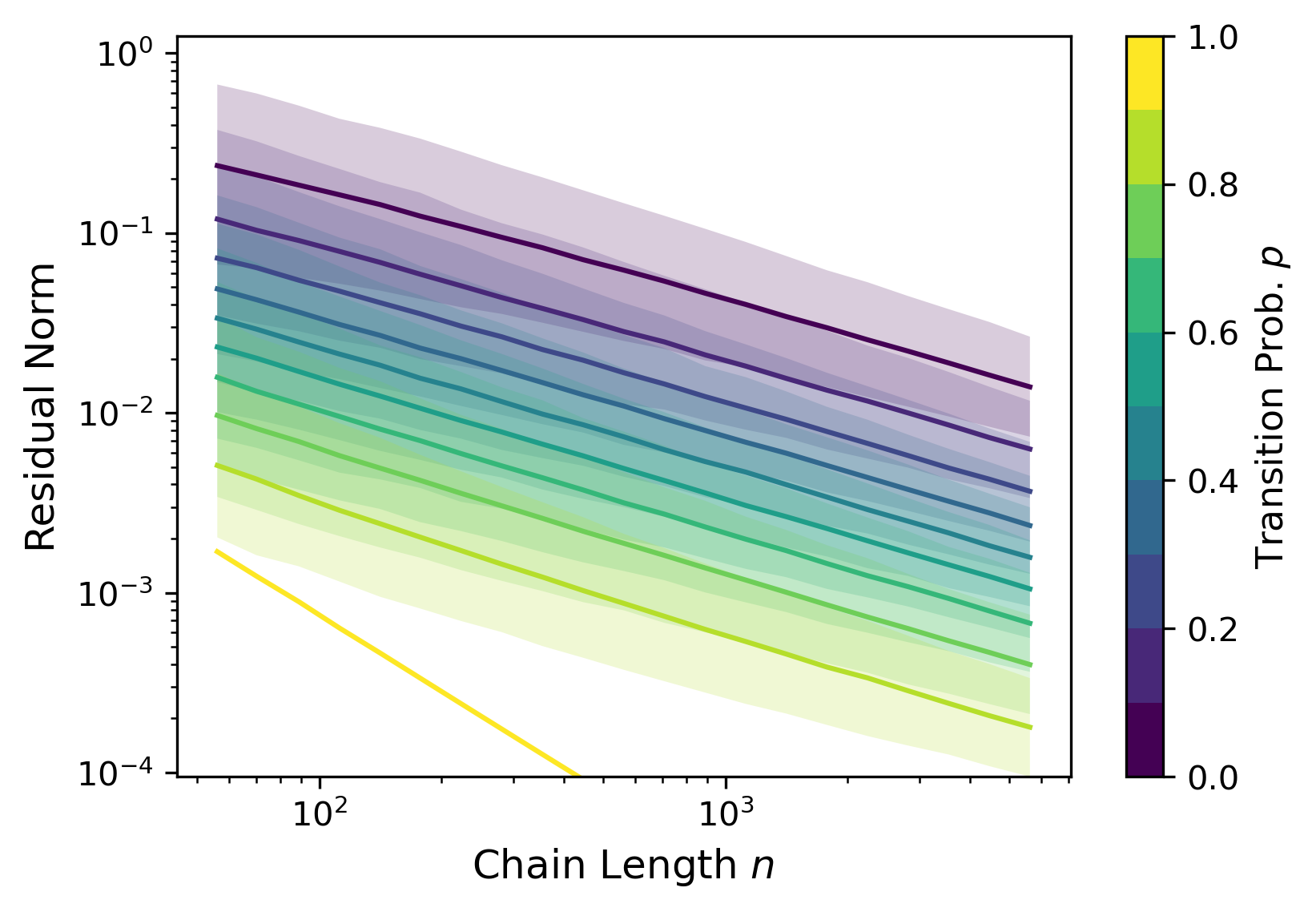
(a) Sobolev-1 with $\tau=n^{-2/3}$.

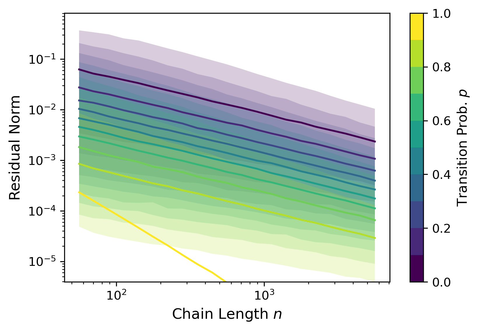
(b) Sobolev-2 with $\tau=n^{-4/5}$.

Figure 10: Residual norm decays $\frac{1}{n}\|\Gamma_{\tau}\bm{\breve{g}}\|_{2}^{2}$, based on the optimal $\tau_{n}$ selections, for different Sobolev-$\alpha$ kernels. Slight numerical inaccuracies are shown in the norm decay of the Sobolev-2 kernel.

The Sobolev-$\alpha$ RKHS on $[0,1]$ has kernel defined by inner product

$$\langle f,g\rangle_{\mathbb{H}^{\alpha}}=\sum_{k=0}^{\alpha}\int_{0}^{1}f^{(k)}(x)\,g^{(k)}(x)\,dx.$$

This Mercer kernel has eigenvalue decay $\lambda_{i}=i^{-2\alpha}$. For the standard KRR problem, a minimax optimal selection of the regularization parameter is given by $\tau_{n}\asymp n^{\frac{-2\alpha}{2\alpha+1}}$. When plugged into the MSE expression,

$$\overline{\rm MSE}(\tau)=\frac{1}{n}\sum_{i=1}^{n}\frac{\tau^{2}\breve{f}_{i}^{2}}{(\lambda_{i}+\tau)^{2}}+\frac{\sigma^{2}}{n}\sum_{i=1}^{n}\frac{\lambda_{i}^{2}}{(\lambda_{i}+\tau)^{2}},$$ (37)

we obtain $\overline{\rm MSE}(\tau_{n})\asymp n^{\frac{-2\alpha}{2\alpha+1}}$ which decays to zero as $n\to\infty$. The resulting rate for $\xi_{n}=\lambda_{n}/\tau_{n}$ is

$$\xi_{n}\asymp n^{\frac{-4\alpha^{2}}{2\alpha+1}}=o(1)$$

which satisfies the condition of Corollary 2. Tying back to Example 2, Figure 10 shows norm decay plots for $\frac{1}{n}\|\Gamma_{\tau}\bm{\breve{g}}\|_{2}^{2}$, when using $\tau_{n}$ minimax selections on the different Sobolev-$\alpha$ kernels.

Similar to the case of the min-kernel in Figure 3, as the signal $\bm{g}^{*}$ becomes more rough, i.e. $p$ becomes larger, we see a quicker decay in filtered norm for the different Sobolev examples. Furthermore, these contributions are filtered at a faster rate for Sobolev kernels that are smoother, that is those with larger $\alpha$ values. This faster decay is not only intuitive but expected from our earlier derived $\xi_{n}$ decay rate.

Appendix C Additional Experiments

Method	# Seqs.	BrainWeb 4-class		BrainWeb 10-class
		Acc. [%]	Max Dev. [1]	Acc. [%]	Max Dev. [1]
k-means	1	$73.62$	$8.21\times 10^{-1}$	$37.69$	$7.08\times 10^{0}$
	3	$74.38$	$3.41\times 10^{0}$	$44.21$	$1.19\times 10^{1}$
N4ITK + k-means	1	$74.10$	$1.17\times 10^{0}$	$40.14$	$6.01\times 10^{0}$
	3	$74.41$	$3.91\times 10^{0}$	$48.22$	$1.11\times 10^{1}$
LapGM	1	$76.14$	$2.87\times 10^{0}$	$50.16$	$\bm{2.47\times 10^{0}}$
	3	$87.28$	$4.08\times 10^{0}$	$78.38$	$\bm{4.19\times 10^{0}}$
AltMin	1	$\bm{91.07}$	$\bm{1.10\times 10^{-1}}$	$\bm{56.27}$	$4.49\times 10^{0}$
	3	$\bm{98.91}$	$\bm{3.67\times 10^{-2}}$	$\bm{82.36}$	$7.84\times 10^{0}$

Table 1: Clustering results for different debiasing methods for single and multi-sequence settings.

We compare AltMin to other MRI debiasing techniques using the same biased phantom as Section 4.2. For comparison, we consider a standard debiasing technique N4ITK [Tustison et al., 2010] and a Bayesian modeling approach LapGM [Vinas et al., 2022]. Hyperparameters for all methods, including AltMin, were selected using the same post-fitting process. Specific to N4ITK, bias estimates were calculated on the T1-sequence information and clusterings were calculated using an additional $k$-means estimation at the end of the debiasing procedure.

Performance of each method for the various recovery settings can be found in Table 1. In each recovery setting, AltMin either meets or exceeds the classification and level accuracies of the other tested methods. We highlight that, for all debias methods, recovery is significantly more difficult in the 10-class setting. Methods which eventually scored well in this setting were those which could effectively leverage multi-sequence information during debias and clustering. This emphasizes the importance of replicated information for practical step and smooth recovery implementations.

References

- Tsybakov [2009] Alexandre B Tsybakov. Introduction to Nonparametric Estimation. Springer, 2009.
- Wainwright [2009] Martin J. Wainwright. Sharp thresholds for high-dimensional and noisy sparsity recovery using 1-constrained quadratic programming (Lasso). IEEE Transactions on Information Theory, 55(5):2183–2202, 2009.
- Bickel et al. [2009] Peter J Bickel, Ya’acov Ritov, and Alexandre B Tsybakov. Simultaneous analysis of Lasso and Dantzig selector. The Annals of statistics, 37(4):1705–1732, 2009.
- Ke et al. [2015] Zheng Tracy Ke, Jianqing Fan, and Yichao Wu. Homogeneity pursuit. Journal of the American Statistical Association, 110(509):175–194, 2015.
- Kim et al. [2009] Seung-Jean Kim, Kwangmoo Koh, Stephen Boyd, and Dimitry Gorinevsky. 1 trend filtering. SIAM Review, 51(2):339–360, 2009.
- Tibshirani [2014] Ryan J. Tibshirani. Adaptive piecewise polynomial estimation via trend filtering. The Annals of Statistics, 42(1):285 – 323, 2014.
- Chandrasekaran et al. [2009] Venkat Chandrasekaran, Sujay Sanghavi, Pablo A. Parrilo, and Alan S. Willsky. Sparse and low-rank matrix decompositions. In 2009 47th Annual Allerton Conference on Communication, Control, and Computing (Allerton), pages 962–967, 2009.
- Bahmani and Romberg [2016] Sohail Bahmani and Justin Romberg. Near-optimal estimation of simultaneously sparse and low-rank matrices from nested linear measurements. Information and Inference: A Journal of the IMA, 5(3):331–351, 05 2016.
- Tanner and Vary [2023] Jared Tanner and Simon Vary. Compressed sensing of low-rank plus sparse matrices. Applied and Computational Harmonic Analysis, 64:254–293, 2023.
- Donoho and Kutyniok [2013] David Donoho and Gitta Kutyniok. Microlocal analysis of the geometric separation problem. Communications on Pure and Applied Mathematics, 66(1):1–47, 2013.
- Hyvärinen and Pajunen [1999] Aapo Hyvärinen and Petteri Pajunen. Nonlinear independent component analysis: Existence and uniqueness results. Neural Networks, 12(3):429–439, 1999.
- Hyvarinen et al. [2019] Aapo Hyvarinen, Hiroaki Sasaki, and Richard Turner. Nonlinear ICA using auxiliary variables and generalized contrastive learning. In Proceedings of the Twenty-Second International Conference on Artificial Intelligence and Statistics, volume 89 of Proceedings of Machine Learning Research, pages 859–868. PMLR, 16–18 Apr 2019.
- Khemakhem et al. [2020] Ilyes Khemakhem, Diederik Kingma, Ricardo Monti, and Aapo Hyvarinen. Variational autoencoders and nonlinear ICA: A unifying framework. In Proceedings of the Twenty Third International Conference on Artificial Intelligence and Statistics, volume 108 of Proceedings of Machine Learning Research, pages 2207–2217. PMLR, 26–28 Aug 2020.
- Zheng et al. [2022] Yujia Zheng, Ignavier Ng, and Kun Zhang. On the identifiability of nonlinear ICA: Sparsity and beyond. In Advances in Neural Information Processing Systems, 2022.
- Asher et al. [2010] Kambiz A Asher, Neal K Bangerter, Ronald D Watkins, and Garry E Gold. Radiofrequency coils for musculoskeletal magnetic resonance imaging. Top. Magn. Reson. Imaging, 21(5):315–323, October 2010.
- Cocosco et al. [1997] Chris A. Cocosco, Vasken Kollokian, Remi K.-S. Kwan, G. Bruce Pike, and Alan C. Evans. BrainWeb: Online interface to a 3D MRI simulated brain database. NeuroImage, 5:425, 1997.
- Vovk et al. [2007] Uro Vovk, Franjo Pernus, and Botjan Likar. A review of methods for correction of intensity inhomogeneity in MRI. IEEE Transactions on Medical Imaging, 26(3):405–421, 2007.
- Kim and Tagare [2014] Yunho Kim and Hemant D. Tagare. Intensity nonuniformity correction for brain mr images with known voxel classes. SIAM Journal on Imaging Sciences, 7(1):528–557, 2014.
- McInnes et al. [2018] Leland McInnes, John Healy, Nathaniel Saul, and Lukas Großberger. Umap: Uniform manifold approximation and projection. Journal of Open Source Software, 3(29):861, 2018. doi: 10.21105/joss.00861. URL https://doi.org/10.21105/joss.00861.
- Lang [1995] Ken Lang. Newsweeder: Learning to filter netnews. In Proceedings of the Twelfth International Conference on Machine Learning, pages 331–339, 1995.
- Wainwright [2019] Martin J. Wainwright. High-Dimensional Statistics: A Non-Asymptotic Viewpoint. Cambridge Series in Statistical and Probabilistic Mathematics. Cambridge University Press, 2019.
- von Luxburg et al. [2008] Ulrike von Luxburg, Mikhail Belkin, and Olivier Bousquet. Consistency of spectral clustering. The Annals of Statistics, 36(2):555 – 586, 2008.
- Prilepin [2023] Eugene Prilepin. csaps. https://github.com/espdev/csaps, 2023.
- Belaroussi et al. [2006] Boubakeur Belaroussi, Julien Milles, Sabin Carme, Yue Min Zhu, and Hugues Benoit-Cattin. Intensity non-uniformity correction in MRI: Existing methods and their validation. Medical Image Analysis, 10(2):234–246, 2006.
- Tustison et al. [2010] Nicholas J. Tustison, Brian B. Avants, Philip A. Cook, Yuanjie Zheng, Alexander Egan, Paul A. Yushkevich, and James C. Gee. N4ITK: Improved N3 bias correction. IEEE Transactions on Medical Imaging, 29(6):1310–1320, 2010.
- Vinas et al. [2022] Luciano Vinas, Arash A. Amini, Jade Fischer, and Atchar Sudhyadhom. LapGM: A multisequence MR bias correction and normalization model, 2022.